Dark-ages Reionization $\&$ Galaxy Formation Simulation II:
Spin and concentration parameters for dark matter haloes during the Epoch of Reionization

Abstract

We use high resolution N-Body simulations to study the concentration and spin parameters of dark matter haloes in the mass range $10^{8}\,{\rm M}_{\odot}\,h^{-1}<{\rm M}<10^{11}\,{\rm M}_{\odot}\,h^{-1}$ and redshifts $5{<}z{<}10$, corresponding to the haloes of galaxies thought to be responsible for reionization. We build a sub-sample of equilibrium haloes and contrast their properties to the full population that also includes unrelaxed systems. Concentrations are calculated by fitting both NFW and Einasto profiles to the spherically-averaged density profiles of individual haloes. After removing haloes that are out-of-equilibrium, we find a $z{>}5$ concentration$-$mass ($c(M)$) relation that is almost flat and well described by a simple power-law for both NFW and Einasto fits. The intrinsic scatter around the mean relation is $\Delta c_{\rm{vir}}{\sim 1}$ (or 20 per cent) at $z=5$. We also find that the analytic model proposed by Ludlow et al. (2014) reproduces the mass and redshift-dependence of halo concentrations. Our best-fit Einasto shape parameter, $\alpha$, depends on peak height, $\nu$, in a manner that is accurately described by $\alpha{=}0.0070\nu^{2}{+}0.1839$. The distribution of the spin parameter, $\lambda$, has a weak dependence on equilibrium state; $\lambda$ peaks at roughly ${\sim}0.033$ for our relaxed sample, and at ${\sim}0.04$ for the full population. The spin–virial mass relation has a mild negative correlation at high redshift.

1 Introduction

In the current cosmological paradigm cold dark matter (CDM) collapses to form gravitationally bound structures within an expanding background universe. Known as dark matter (DM) haloes, these objects are initially small but undergo repeated merging to form ever larger systems. Galaxies form within these haloes as in-falling gas cools and converts to stars (e.g. White & Rees, 1978). Their evolution and structural properties therefore underpin those of the embedded galaxies. These ideas have evolved into the field of semi-analytic modelling in which galaxies are grown within an evolving population of dark-matter haloes extracted from purely N-Body simulations (e.g. Croton et al., 2006; Somerville et al., 2008; Lagos et al., 2008, see Baugh 2006 for a review).

The characteristics of DM haloes have been the subject of extensive research. Mass determines the overall size of the halo, but several other important parameters have also been identified. For example, using N-Body simulations (Navarro et al., 1997, henceforth NFW) found that the density profiles of virialised haloes can be well described by rescaling a simple formula (hereafter known as the NFW profile):

$$\frac{\rho(r)}{\rho_{\rm{c}}}=\frac{\delta_{\rm{c}}}{(r/r_{\rm{s}})(1+r/r_{\rm{s}})^{2}}.$$ (1)

Here $r_{\rm{s}}$ is the characteristic scale radius at which the logarithmic density slope is equal to -2; $\delta_{\rm{c}}$ is the characteristic density contrast, and $\rho_{\rm c}=3\,H(z)^{2}/8\pi G$ the critical background density at redshift $z$, where G is Newton’s gravitational constant and $H$ the Hubble parameter. These parameters can be expressed in a variety of forms. One common approach is to use a virial mass, and concentration, $c_{\rm{vir}}\equiv R_{\rm{vir}}/r_{\rm{s}}$, defined as the ratio of the halo’s virial radius to its scale radius.

While the NFW profile is a common description, several recent studies (e.g. Navarro et al., 2004; Hayashi & White, 2008; Navarro et al., 2010) have shown that the density profiles of simulated haloes exhibit small but systematic deviations from eq. 1. The Einasto profile (Einasto, 1965), defined

$$\ln\biggl{(}\frac{\rho_{\rm Ein}(r)}{\rho_{-2}}\biggl{)}=-\frac{2}{\alpha}\biggl{[}\biggl{(}\frac{r}{r_{-2}}\biggl{)}^{\alpha}-1\biggl{]},$$ (2)

provides a better approximation to the radial density profile (Navarro et al., 2004; Ludlow et al., 2013). Like the NFW profile, eq. 2 has two scaling parameters, $r_{-2}$ and $\rho_{-2}$, and an additional shape parameter, $\alpha$. Note that $r_{-2}$ and $r_{s}$ are equivalent, and we will hereafter use the two interchangeably when defining the concentration of a halo.

At low redshift the concentration parameter decreases with increasing halo mass. NFW interpreted this finding as a result of hierarchical clustering: smaller haloes form earlier than more massive objects, when the universe was denser. They suggested that concentration, or equivalently the characteristic density, $\delta_{c}$, reflects the background density of the Universe at the halo’s formation time.

The same negative trend was also seen in subsequent N-Body simulations (e.g. Eke et al., 2001; Wechsler et al., 2002; Duffy et al., 2008), and lead to the development of analytic models attempting to explain the dependence of concentration on mass, redshift and cosmology. One approach relates $\delta_{c}$ to the past accretion history of the halo’s main progenitor. Wechsler et al. (2002), for example, calculated the mass assembly histories (MAHs) of simulated haloes and used a proportionality constant to relate the concentration to background density at the halo’s time of formation, defined by the point at which the logarithmic accretion rate falls below a specific value. The redshift dependence of the $c(M)$ relation was later studied by Zhao et al. (2003), who found a weakening of the relation for the highest mass haloes at any redshift. By $z{\sim}$3-4 the negative trend is no longer present in the simulations of Gao et al. (2008), who focus on masses $M>10^{11}{\rm M}_{\odot}/h$. The flattening of the $c(M)$ relation was also reported by Zhao et al. (2009) who connected halo concentrations to the period at which halo growth transitions from a rapid to a slow phase. Although these models have been met with limited success overall, they provide a clear interpretation of why concentration depends only weakly on mass for the most massive systems: because these haloes are forming today, they share the same formation time, and therefore concentration.

Neto et al. (2007) studied the $z=0$ $c(\rm{M})$ relation in the Millennium simulation (Springel et al., 2005), while Klypin et al. (2011) and Prada et al. (2012) extended the analysis to $z=6$ using both the Millennium and Bolshoi simulations. In agreement with previous work, these authors each find a decline of concentration with mass. However, both Prada et al. (2012) and Klypin et al. (2011) have also reported an upturn of the $c({\rm M})$ relation at the high mass end. On the other hand, Ludlow et al. (2012) demonstrated that there is no upturn amongst relaxed haloes, and showed how the transient dynamical states of merging systems can result in a non-monotonic $c({\rm M})$ relation. While the details continue to be debated, it is clear overall that the diversity of halo formation histories play a critical role in establishing the shape and evolution of the $c({\rm M})$ relation (Ludlow et al., 2014; Correa et al., 2015).

While the low redshift mass-concentration relation is well studied, at high $z$ the relation is poorly constrained. For example, Prada et al. (2012) and Diemer & Kravtsov (2014) find a high-mass upturn (above a few times $10^{10}\,h^{-1}\,{\rm M}_{\odot}$) at $z=5$ amongst the full halo population. At similar masses, Dutton & Macciò (2014), find a relation with a slightly positive slope, whereas Hellwing et al. (2015) report a weak negative slope that flattens by $z{=}9$. These authors, however, imposed different equilibrium cuts on their halo samples, which hampers a direct comparison with their results. Given this unsettled state of affairs it is clear that there is some debate on the precise nature of the high redshift $c(\rm{M})$ relation and the role played by unrelaxed haloes.

For example, a halo suffering a merger is unlikely to have a simple, smooth density profile, and will take time to settle back into equilibrium. This situation becomes increasingly important at high redshift due to the elevated merger rates of potentially star-forming haloes. These sorts of concerns led Neto et al. (2007) to introduce three physically-motivated parameters to identify systems far from equilibrium: 1) the mass-fraction in substructure $f_{\rm{sub}}={\rm M_{sub}}(<{\rm R_{vir}})/{\rm M_{vir}}$; 2) the offset between the halo’s center of mass and its most-bound particle, $x_{\rm{off}}$, and 3) the pseudo-virial-ratio of kinetic and potential energies, $\varphi$. The effectiveness of these parameters in isolating relaxed DM haloes is further discussed in Gao et al. (2008) and Ludlow et al. (2012).

A detailed study of these parameters with regard to dynamical relaxation at high redshift is provided by the first paper of the DRAGONS series, Poole et al. (2015b) (hereafter referred to as Paper I), who examine the behaviour of these equilibrium diagnostics during the relaxation phase that follows a significant merger or accretion event during the Epoch of Reionization. Their results suggest that, across the mass range of our simulations, $10^{8}<{\rm M}/[h^{-1}\,{\rm M}_{\odot}]<10^{11}$, and for $z>5$, standard relaxation values for $f_{\rm{sub}}$, $x_{\rm{off}}$ and $\varphi$ obtained from low redshift studies are very effective at identifying systems relaxing from halo formation or recent mergers at high redshift.

Concentration is not the only relevant halo property for galaxy formation. Halo spin also plays an important role in semi-analytic models, since angular momentum conservation determines the size of galactic disks (e.g. Mo et al., 1998; Guo et al., 2011), which in turn determine their star formation rates (Schmidt, 1959; Kennicutt, 1998). A halo’s angular momentum is often expressed as a dimensionless spin parameter:

$$\lambda=\frac{J_{\rm{vir}}}{\sqrt{2}M_{\rm{vir}}V_{\rm{vir}}R_{\rm{vir}}},$$ (3)

where $J_{\rm{vir}}$ is the total angular momentum within ${\rm R_{vir}}$.

Most studies of the spin parameter have focused on the distribution of spins and its dependence on halo mass (e.g. Bett et al., 2007; Neto et al., 2007; Knebe & Power, 2008; Muñoz Cuartas et al., 2010). At any redshift, halo spins are distributed approximately log-normally, and peak at $\lambda_{0}{\sim}0.03{-}0.04$. At low redshift, spins are approximately independent of mass but gain a slight negative correlation at higher redshifts (Knebe & Power, 2008; Muñoz Cuartas et al., 2010). Recently, Dutton & Macciò (2014) measured the redshift evolution of the $\lambda-M_{\rm{vir}}$ relation, reporting a weak negative correlation at $z=5$.

In this work we use the Tiamat simulation suite to extend the study of concentration and spin to redshifts $z>5$. Our simulations were designed to resolve halo masses relevant for galaxy formation during this high-redshift epoch. The purpose of our study is to measure the structural and dynamical properties of haloes that are necessary for forthcoming semi-analytic models of reionization.

We organise the paper as follows. In Section 2 we describe the numerical simulations, including halo finding, analysis techniques, and our parametrization of concentration and spin. In Section 3 we present our concentration–mass relation and its redshift dependence, and in Section 4 the spin distribution, and its mass and redshift dependence. Finally, in Section 5 we summarise our main results.

2 Numerical Simulation

Our analysis focuses on DM haloes identified in three cosmological N-body simulations. These include a 2160³-particle, 67.8 Mpc$/h$ cubed box (the Tiamat simulation) and two smaller but higher resolution volumes of 10 and 22.6 (Mpc$/h$)³. Each run was carried out with GADGET-2 (Springel et al., 2001b; Springel, 2005) with RAM (random-access memory) consumption changes in accordance with those detailed in Poole et al. (2015). For each run, the Plummer-equivalent softening length was $1/50^{\rm{th}}$ of the mean Lagrangian inter-particle spacing, and the integration accuracy parameter, $\eta$, is set to 0.025, as motivated by the convergence study presented in Poole et al. (2015). Initial conditions were generated using 2nd order perturbation theory (using the code 2LPTic, Crocce et al., 2006) at $z=99$ and each simulation was run down to $z=5$; 100 snapshots of particle data were taken equally spaced in time from $z=35$ to $z=5$ (one every 11 Myr). Cosmological parameters for each box were chosen to be consistent with the Planck 2015 data release (Planck Collaboration et al., 2015) $(h,\Omega_{\rm{m}},\Omega_{\rm{b}},\Omega_{\Lambda},\sigma_{8},n_{\rm{s}})$ = $(0.678,0.308,0.0484,0.692,0.815,0.968)$. The relevant numerical parameters are summarised in Table 1. A more detailed discussion of these simulations can be found in Paper I.

Simulation	$N_{\rm{p}}$	L [Mpc$/h$]	$m_{\rm{p}}$ [$\rm{M}_{\odot}/h$]	$\epsilon$ [kpc$/h$]
Tiamat	$2160^{3}$	67.8	$2.64{\times}10^{6}$	0.63
Medi Tiamat	$1080^{3}$	22.6	$7.83{\times}10^{5}$	0.42
Tiny Tiamat	$1080^{3}$	10.0	$6.79{\times}10^{4}$	0.19

Table 1: Summary of simulation parameters. $N_{\rm{p}}$ is the total number of particles, L is the length of the box, $m_{\rm{p}}$ is the mass of each particle and $\epsilon$ is the gravitational force softening length.

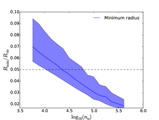
Figure 1: The ratio between the minimum bin size of the halo profile in dark blue and the size of the virial radius, plotted as a function of particle number for the Tiamat simulation. The solid line is the median while the shaded area is the scatter (68 per cent confidence interval). The largest bin size of $0.09R_{\rm{vir}}$ indicates our bins begin well inside the halo scale radius for the halo masses considered here.

2.1 Halo Finding

Haloes were identified in each simulation snapshot using Subfind (Springel et al., 2001a). This produces two outputs: the first contains structures found by a friends-of-friends (FoF) algorithm (we adopt a linking length of 0.2 times the mean inter particle spacing); the second is obtained by dissecting each FoF group into its self-bound “substructure”. This results is a central “main halo”, typically containing $>90$ per cent of its virial mass, and a group of lower-mass subhaloes which trace the undigested cores of previous merger events.

Each main halo and its substructures were further analyzed to catalog their basic properties and to build their spherically averaged profiles. A (FoF or substructure) halo was required to have a at least 32 particles to be included, resulting in a minimum halo mass of $8.4\times 10^{7}\rm{M}_{\odot}/h$ in Tiamat, $2.5\times 10^{7}\rm{M}_{\odot}/h$ in Medi Tiamat and $2.2\times 10^{6}\rm{M}_{\odot}/h$ in Tiny Tiamat. However, when estimating concentrations, a stricter limit of $n_{\rm{p}}{>}5000$ within the bound structure was imposed to ensure that the halo’s inner regions are well-resolved. For the purpose of estimating spin parameters, this limit is relaxed to 600 particles. These parameter choices are further discussed and motivated in Section 2.3.

2.2 Density Profiles and Concentration Estimates

For each main halo, spherically-averaged density profiles were constructed in bins containing an equal number of particles. Only particles considered by Subfind to be bound to the central haloes were used. The number of bins was increased along with the number of halo particles. We imposed a minimum of 5 bins for the smallest haloes, and a maximum of 1000 bins for the largest (reached as $n_{\rm{p}}$ tends to $10^{6}$). For example, haloes with $n_{\rm{p}}{=}$ 5000 have 25 bins, rising to ${\sim}$125 bins for haloes containing $10^{5}$ particles.

Best-fit NFW and Einasto profiles were obtained by minimizing

$$\psi=\frac{1}{N}\sum\limits_{\rm{i}}^{\rm{N}}\frac{\Delta r_{\rm{i}}}{r_{\rm{i}}}(\log\rho_{\rm{i}}-\log\rho_{\rm{NFW(Ein)}})^{2},$$ (4)

where N is the number of bins, $\rho_{\rm{i}}$ is the density in bin $i$, and $\rho_{\rm{NFW(Ein)}}$ is the corresponding density of the NFW (Einasto) model. The factor $\Delta r_{\rm{i}}/r_{\rm{i}}$ (the width of bin $i$ divided by the median radius of particles in it) appropriately weights bins of differing size. Note that only bins in the radial range $0.05R_{\rm{vir}}<r_{i}<0.8R_{\rm{vir}}$ were used (we have verified that the minimum bin radius is always larger than the convergence radius defined in Power et al., 2003).

In Figure 1 we show the ratio of the minimum bin size to the halo virial radius. For the smallest resolved haloes ($n_{\rm{p}}{=}$ 5000) this ratio falls to ${\sim}$ 12, and thus scale radii corresponding to concentrations as high as 12 could be resolved even for the smallest haloes considered. We find concentrations are almost always ${<}$10. This indicates that our bins span a sufficient portion of the halo profile to provide reliable estimates of $r_{\rm{s}}$.

2.3 Resolution and Virialisation Cuts

In defining our sample of equilibrium DM haloes we impose both dynamical and resolution criteria following the procedure established by Neto et al. (2007), Gao et al. (2008) and Ludlow et al. (2012). The behaviour of these equilibrium diagnostics over the mass and redshift range probed by the Tiamat simulation suite is discussed further in Paper I. The criteria defining relaxed haloes include upper limits on the following three quantities:

1. The fraction of mass found in satellite subhaloes, $f_{\rm{sub}}=M_{\rm{sub}}(<R_{\rm{vir}})/M_{\rm{vir}}<0.1$. As discussed in Neto et al. (2007) a high fraction of mass in substructure may be indicative of a recent merger. Such a halo will not, in general, have a smooth, spherically-averaged density profile.

2. The offset between the position of the most-bound-particle, $\vec{r}_{\rm{mbp}}$, and center-of-mass, $\vec{r}_{\rm{com}}$, in units of virial radius: $x_{\rm{off}}=|\vec{r}_{\rm{mbp}}-\vec{r}_{\rm{com}}|/R_{\rm{vir}}<0.07$. This is complementary to $f_{\rm{sub}}$ as it includes mass from unresolved subhaloes, or merging haloes that have their center just outside the virial radius and consequently are not included in $f_{\rm{sub}}$.

3. The pseudo-virial ratio of kinetic and potential energies, $\varphi=2K/|U|<1.35$. This criterion tends to be sensitive to haloes at the pericenter of a merger that may not be flagged by the above two parameters.

Neto et al. (2007) find that these restrictions, although arbitrary in value, provide a simple and physically motivated method to exclude haloes that are not well described by an NFW profile. In Paper I these parameters were also shown to be discriminate between haloes that have either recently doubled in mass, or suffered a major or minor merger, within the last $1{-}2$ dynamical times. We therefore adopt them as our standard equilibrium criteria, and use them to split our full halo sample into a relaxed sub-sample, which we analyse separately.

A further criterion is imposed to select only well-resolved haloes from both the relaxed and unrelaxed populations, in order to fit a reliable radial halo profile. For the halo concentration analysis a lower limit on particle number ($n_{\rm{p}}$) of $n_{\rm{p}}{>}5000$ is imposed. This is derived from work studying convergence of NFW and Einasto profile fits in Neto et al. (2007) and Gao et al. (2008). This ensures that the inner portion of the halo is well enough resolved to measure the scale radius $r_{\rm{s}}$. We impose a restriction of $n_{\rm{p}}>600$ particles for the spin parameter measurement following Knebe & Power (2008), who obtain the limit by comparing the measured energy from Monte Carlo realisations of analytic NFW profiles.

The dynamics of hierarchical growth means that at the high redshifts studied here, many of our haloes will be far from equilibrium and thus have ill-defined values for concentration and spin. These sample cuts are designed to remove such systems and to keep transients out of our analysis as much as possible. For example, a halo which has just undergone a major merger may be comprised of two large, high density clumps, and consequently have a high $x_{\rm{off}}$ and poorly defined center. The density profile of such a system cannot be captured by simple spherical averages, and structural properties estimated from NFW or Einasto fits are meaningless. We stress, however, that there is a continuum of values for $x_{\rm{off}}$, $f_{\rm{sub}}$ and $\varphi$; the particular values chosen to separate relaxed haloes from unrelaxed are the result of extensive past investigations (see, e.g., Neto et al., 2007; Ludlow et al., 2012, and Paper I of this series). Our choices of resolution and dynamical classification also simplify comparison with previous studies.

To quantify the effects of our sample selection, we note that in Tiamat there are 14391 haloes with more than 5000 particles at redshift $z\sim 5$, but only 4433 (or $\sim$30 per cent) of these satisfy our relaxation criteria; this reduces to $\sim$15 per cent by $z\sim 10$. These numbers underline the importance of the dynamical state of haloes at high redshift. Nevertheless parametrised fits to the entire population are useful for many semi-analytic calculations (e.g. Mack, 2014; Schön et al., 2015) and for this reason we report fits to both our full halo sample as well as the relaxed sub-sample. Further details regarding the dynamical state of high redshift haloes are presented in Paper I.

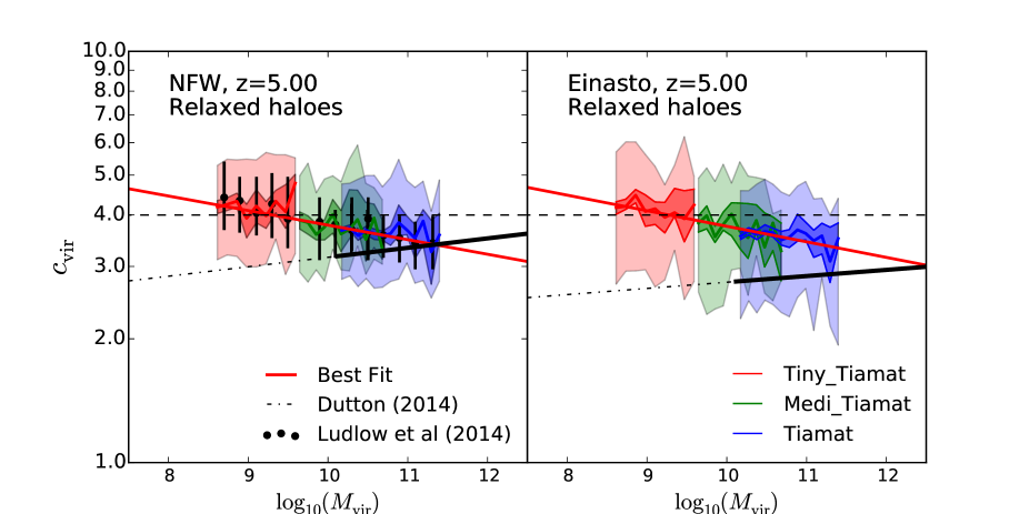
Figure 2: Concentration–mass relation of relaxed central haloes at $z{=}5$. Left and Right panels are the NFW and Einasto concentrations respectively. Inner shaded region denotes the bootstrapped 90 per cent confidence interval on the median. The outer shaded region shows the $68$ per cent scatter. The line of best fit is fit to the median using the Monte Carlo Markov Chain method implemented in the Python package emcee (Foreman-Mackey et al., 2013). This produces $c_{\rm{vir}}=3.8\pm 0.4(\rm{M}/[10^{10}\rm{M}_{\odot}h^{-1}])^{-0.035\pm 0.005}$ at $z{=}5$ for NFW fits and $c_{\rm{vir}}=3.8\pm 0.4(\rm{M}/[10^{10}\rm{M}_{\odot}h^{-1}])^{-0.039\pm 0.005}$ for Einasto fits. The fits from Dutton & Macciò (2014) are also shown with thick solid lines representing fitting formula over their derived mass range, although we emphasise Dutton & Macciò (2014) employ different relaxation and resolution criteria for their sample. Thin extensions of these lines represent these fits extrapolated to lower masses. The Tiamat simulation is designed to study reionization and explores a mass range below previous studies. The dashed black line at $c_{\rm{vir}}=4$ is added for a point of reference. Solid black points represent the Ludlow et al. (2014) model where halo concentrations are calculated from the median accretion history in the mass bin. Error bars are derived from the 68 per cent scatter in accretion histories.

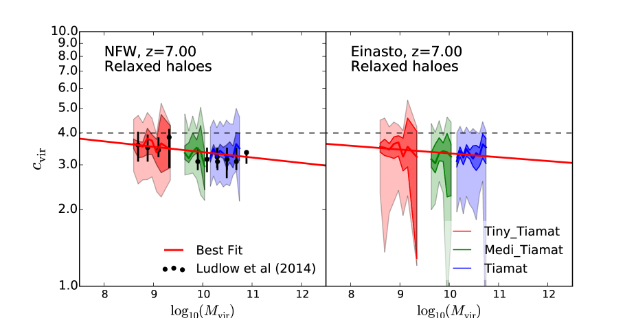
Figure 3: The same concentration mass relations for relaxed central haloes as shown in Figure 2, but now at $z{=}7$. Inner shaded region denotes the bootstrapped 90 per cent confidence interval on the median. The outer shaded region shows the $68$ per cent scatter. The line is fit to the median and gives $c_{\rm{vir}}$ = $3.4\pm 0.6(\rm{M}/[10^{10}\rm{M}_{\odot}h^{-1}])^{-0.019\pm 0.008}$ at $z{=}7$ for NFW and $3.3\pm 0.6(\rm{M}/[10^{10}\rm{M}_{\odot}h^{-1}])^{-0.018\pm 0.008}$ for Einasto profiles. The dashed black line at $c_{\rm{vir}}=4$ is added for a point of reference. Solid black points represent the Ludlow et al. (2014) model where halo concentrations are calculated from the median accretion history in the mass bin. Error bars are derived from the $68$ per cent scatter of the accretion histories.

3 Concentration Mass Relation

3.1 The concentration mass relation for relaxed haloes

The $c(M)$ relations for our equilibrium haloes at $z{=}5$ and $z{=}7$ are shown in Figures 2 and 3, respectively. Both NFW and Einasto concentrations are plotted. The inner shaded region shows the bootstrapped 90 per cent confidence interval on the median for mass bins containing at least 20 haloes. The outer shaded area fills the 68 per cent scatter in individual concentration estimates. We find a weak trend of decreasing concentration with mass at $z{=}5$ for both NFW and Einasto fits. This trend becomes shallower as redshift increases. By redshift 9 there is no trend apparent for either set of fits (see Table 2). The $c({\rm M})$ relations obtained from both NFW and Einasto fits are similar over this mass range. We note that the systematic difference between NFW and Einasto concentrations is $\Delta c_{\rm{vir}}<$0.1, which is smaller than the change in concentration from the lowest to highest masses studied here.

Best-fitting power laws at $z{=}5$ are $3.8\pm 0.4\,({\rm M}/[10^{10}\,h^{-1}\,{\rm M}_{\odot}])^{-0.039\pm 0.005}$ for NFW fits and $3.8\pm 0.4\,({\rm M}/[10^{10}\,h^{-1}\,{\rm M}_{\odot}])^{-0.039\pm 0.005}$ for Einasto fits. Best-fit parameters are obtained using the Monte Carlo Markov Chain (MCMC) method implemented with the emcee package (Foreman-Mackey et al., 2013). The quoted errors are the $68$ per cent confidence interval derived from the posterior distribution. We find intrinsic scatter in the $c({\rm M})$ relation of $\Delta c_{\rm{vir}}\sim 1.0$ (or 20 per cent) for fits to both NFW and Einasto profiles. Best-fit power-law relations (for both NFW and Einasto fits) are provided in Table 2 for a range of redshifts.

In addition to the two scaling variables, the Einasto profile has a shape parameter, $\alpha$. Previous studies have found that $\alpha$ depends in a complex way on both halo mass and redshift, but follows a simple relation when expressed in terms of the dimensionless “peak height” mass parameter, $\nu=\delta_{\rm sc}/\sigma({\rm M},z)$. Here $\delta_{\rm sc}=1.686$ is the density threshold for the collapse of a spherical top-hat density perturbation, and $\sigma({\rm M},z)$ is the rms density fluctuation in spheres enclosing mass ${\rm M}$. Figure 4 shows the $\alpha-\nu$ relation obtained from our Einasto fits. We find a similar $\alpha-\nu$ relation to the previous authors – the fit from Gao et al. (2008) is shown as a dashed line – although our simulations cover a different mass and redshift range. Our best fit for the $\alpha-\nu$ relation is $\alpha=0.007\nu^{2}+0.1839$.

In order to check for any subtle bias in our fits we have also constructed $c({\rm M})$ and $\alpha(\nu)$ relations using the median density profiles obtained by stacking haloes in narrow mass bins. This smooths out any unique features of individual systems and allows for a robust estimate of the median structural properties of haloes of a given mass. For our relaxed population we recover the $c({\rm M})$ to within $\Delta c{\sim}0.1$, for both NFW and Einasto fits. We choose to use the individual fits when computing the best fit $c({\rm M})$ relation.

The weak trend in concentration with mass found in our simulation is in qualitative agreement with previous work that found a negative trend at low redshift that becomes progressively shallower with increasing $z$. For example, both the shallow negative slope and the magnitude of our Einasto concentrations are in good agreement with Hellwing et al. (2015).

In Figure 2 we also plot the $c({\rm M})$ relations from Dutton & Macciò (2014) (hereafter DM14), also obtained from both NFW and Einasto fits. The mass range covered by their simulations is shown as the thick solid line, while the thin dot-dashed line is an extrapolation. As DM14 employ different relaxation and resolution criteria, the differences we observe, although slight, are unsurprising. However, the shape of our trend at redshift 5 is in qualitative disagreement with DM14, who find that a positive trend emerges at $z{=}5$ for both Einasto and NFW concentrations. We also find a higher normalization (about 25 per cent) than DM14 at ${\sim}10^{10}M_{\odot}h^{-1}$.

The method of our analysis differs in a few significant ways from DM14. We do not speculate on the exact combination of these differences that effects the $c({\rm M})$ relation but note that: firstly, halo profiles in DM14 are fit out to 1.2$R_{\rm{vir}}$ while Tiamat profiles are only fit out to 0.8$R_{\rm{vir}}$, and second, different resolution and relaxation criteria were used. DM14 adopt a minimum halo mass corresponding to 500 particles, and define relaxed haloes as those satisfying $x_{\rm{off}}<0.07$ and $\rho_{\rm{rms}}<0.5$, where

$$\rho_{\rm{rms}}=\sqrt{\frac{1}{\rm{N}}\sum^{\rm{N}}_{i}(\ln\rho_{\rm{i}}-\ln\rho_{\rm{\rm{Fit}}})^{2}}$$ (5)

is the rms deviation between the haloes density profile and the best-NFW fit.

However, we do find good agreement between our $c({\rm M})$ relation results and the model proposed by Ludlow et al. (2014), as indicated by the black dots in Figures 2 and 3. The black dots are obtained by finding the median scale radius such that the mean density within this radius is equal to ${\sim}725$ times the critical density when its progenitor first achieved this mass, i.e. $<\rho>=725\times\rho_{\rm{crit}}$ (Ludlow et al., 2013). In Ludlow et al. (2013) this relation is actually $<\rho>=776\times\rho_{\rm{crit}}$, as it is calibrated using a different cosmology, and to the $M_{200}$ defintion of mass. We adjust this relation to $<\rho>=725\times\rho_{\rm{crit}}$ to allow for our use of the $M_{\rm{vir}}$ mass definition and the different cosmology of Tiamat. This reproduces our median $c({\rm M})$ relations. We emphasise there is no fit to the halo density profiles here, only the accretion histories are required.

$z$	Relaxed NFW Best Fit	Relaxed Einasto Best Fit	$N_{\rm{sample}}$
5	$(3.8\pm 0.4)(\frac{M}{10^{10}M_{\odot}h^{-1}})^{(-0.035\pm 0.005)}$	$(3.8\pm 0.4)(\frac{M}{10^{10}M_{\odot}h^{-1}})^{(-0.039\pm 0.005)}$	4443,738,864
6	$(3.6\pm 0.5)(\frac{M}{10^{10}M_{\odot}h^{-1}})^{(-0.023\pm 0.006)}$	$(3.5\pm 0.5)(\frac{M}{10^{10}M_{\odot}h^{-1}})^{(-0.022\pm 0.007)}$	2303,412,652
7	$(3.4\pm 0.6)(\frac{M}{10^{10}M_{\odot}h^{-1}})^{(-0.019\pm 0.008)}$	$(3.3\pm 0.6)(\frac{M}{10^{10}M_{\odot}h^{-1}})^{(-0.018\pm 0.008)}$	1043,221,417
8	$(3.3\pm 1.0)(\frac{M}{10^{10}M_{\odot}h^{-1}})^{(0.005\pm 0.013)}$	$(3.3\pm 1.2)(\frac{M}{10^{10}M_{\odot}h^{-1}})^{(0.013\pm 0.016)}$	391,109,267
9	$(3.2\pm 1.2)(\frac{M}{10^{10}M_{\odot}h^{-1}})^{(0.003\pm 0.016)}$	$(3.2\pm 1.5)(\frac{M}{10^{10}M_{\odot}h^{-1}})^{(0.003\pm 0.021)}$	134,49,155

Table 2: Best fit values from the relaxed population for NFW-derived and Einasto-derived $c({\rm M})$ relations $c_{\rm{vir}}$ = $A(\rm{M_{\rm{vir}}}/[10^{10}M_{\odot}h^{-1}])^{B}$. $N_{\rm{sample}}$ denotes the number of haloes in the sample for $\textit{Tiamat},\textit{Medi Tiamat},\textit{Tiny Tiamat}$. Fits and errors are the median and 68 per cent confidence interval using the MCMC package quoted previously.

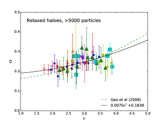
Figure 4: The Einasto profile $\alpha-\nu$ relation. At each redshift the median $\alpha$ is plotted for bins containing $>20$ haloes, with the errors derived from the bootstrapped $90$ per cent confidence interval on the median. Each symbol denotes a different redshift; red pluses denote $z{=}5$, blue filled circles denote $z{=}6$, green triangles denote $z{=}7$, yellow stars denote $z{=}8$, cyan squares denote $z{=}9$ and magenta inverted (point down) triangles denote $z{=}10$. We find a similar $\alpha-\nu$ relation to the low redshift results of previous authors despite the redshift range of our simulations being $z>5$.

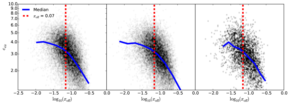
Figure 5: The dependence of concentration on $x_{\rm{off}}$ for central subgroups in several mass ranges. From left to right the ranges are [$10^{10.0}\rm{M}_{\odot}/h<M<10^{10.5}\rm{M}_{\odot}/h$], [$10^{10.5}\rm{M}_{\odot}/h<M<10^{11.0}\rm{M}_{\odot}/h$] and [$10^{11.0}\rm{M}_{\odot}/h<M<10^{11.5}\rm{M}_{\odot}/h$]. Blue lines represent the median. The dashed red line denotes the relaxation criteria cut above which a halo is considered to be out of equilibrium (Neto et al., 2007; Gao et al., 2008; Ludlow et al., 2012, Paper I). It can be seen that lower $x_{\rm{off}}$ parameters (i.e. more relaxed haloes) correlate with higher $c_{\rm{vir}}$ for all mass ranges.

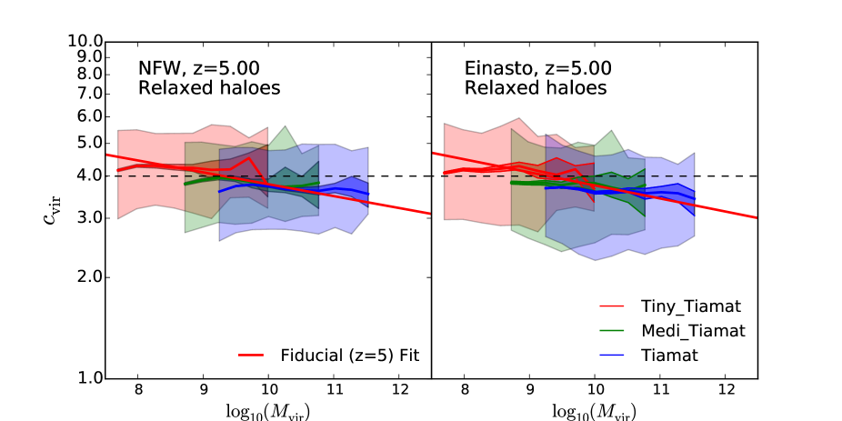
Figure 6: Concentration–mass relation for relaxed haloes at $z{=}5$, but now with haloes containing ${>}$500 particles. The inner shaded region represents the bootstrapped median value and the outer region the $68$ per cent scatter. Dashed black line is the $c_{\rm{vir}}=4$ line for reference and the fiducial red line is the best fit to the relaxed population as in Figure 2. The inclusion of haloes with particles number ${<}$5000 introduces more haloes with lower concentrations at the low mass end of each simulation. Einasto shape parameters, $\alpha$, for haloes with ${<}$500 particles are also higher as seen in Figure 8.

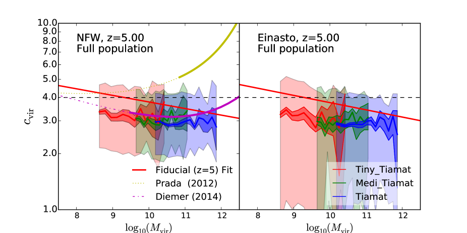
Figure 7: The same as Figure 2 but now the case in which no non-equilibrium cuts are enforced and the full sample of haloes with ${>}$5000 particles is analysed. The inner shaded region represents the bootstrapped median value and the outer region the $68$ per cent scatter. The dashed black line at $c_{\rm{vir}}=4$ is added for a point of reference and the fiducial red line is the best fit to the relaxed population as in Figure 2. The thick solid line represents previous authors’ fits in the mass range their simulations cover, while the thin solid line is the extrapolation to lower masses. The median magnitude of the concentrations has decreased by $\Delta c_{\rm{vir}}\sim 1$ over all masses in our simulations.

3.2 Effects of relaxation and resolution

To investigate the effect of our equilibrium selection criteria we plot in Figure 5 the variation of concentration with $x_{\rm{off}}$, the most restrictive of the three. There is a clear trend that haloes with higher $x_{\rm{off}}$ have lower concentrations, representing a $\Delta c_{\rm{vir}}\sim 2$ decrease for haloes with the largest offsets (${\sim}30$ per cent of the virial radius). The trend is similar at all three of the mass ranges considered. This figure illustrates how important it is to understand the dynamical state of the haloes included in the sample.

In Figures 6 and 7 we again present the $c({\rm M})$ relation but now relax the strict resolution and equilibrium criteria. Firstly, in Figure 6 we show the relation that results from lowering the minimum particle limit for a halo to 500 particles, while maintaining the relaxation criteria. Whereas our $n_{\rm{p}}{>}5000$ relation agreed where simulations overlapped, we find a significant discrepancy between the simulations for masses corresponding to haloes with $5000>n_{\rm{p}}>500$. In particular, lower particle numbers result in lower values of $c_{\rm{vir}}$. For Einasto profiles the $\alpha-\nu$ relation also changes slightly, as shown in Figure 8. Many of the $500<n_{\rm{p}}<5000$ haloes have $\alpha\sim 0.25$ and do not follow the previous quadratic $\alpha-\nu$ relation. We thus caution against over-interpreting Einasto fit parameters at low particle number.

In Figure 7 the $c({\rm M})$ relation is plotted for the entire halo sample. At all masses, the median concentrations decrease relative to those of our relaxed haloes. We also note that inclusion of unrelaxed haloes alters the $\alpha-\nu$ relation slightly. Our best-fit to the full population is $\alpha=0.0091\nu^{2}+0.1447$, which is slightly steeper than that found by Duffy et al. (2008) when they include unrelaxed haloes. Table 3 shows the best fit parameters for the full population of resolved haloes with $n_{\rm{p}}{>}500$ particles.

In the left hand panel of Figure 7 we also plot the models of Diemer & Kravtsov (2014) and Prada et al. (2012), where we have analytically adjusted the Prada et al. (2012) relation from the $c_{200},M_{200}$ definitions, which they use, to the $c_{\rm{vir}},M_{\rm{vir}}$ defintions used in this work by assuming an NFW profile. Diemer & Kravtsov (2014) use the phase space halo finder ROCKSTAR (Behroozi et al., 2013), and do not enforce any relaxation criteria. They also utilise different resolution criteria. The mass range covered in Diemer & Kravtsov (2014) is equivalent to the mass range covered by Tiamat with halo particle numbers of $n_{\rm{p}}{>}1200$. In this mass range we see slight evidence for an upturn in the Tiamat $c({\rm M})$ relation, which is consistent with their findings. Note that this upturn is a feature exclusive to our full halo sample, suggesting its connection to departures from equilibrium.

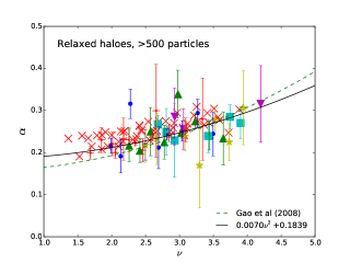
Figure 8: The Einasto $\alpha-\nu$ relation but including haloes above $n_{\rm{p}}>500$ particles. At each redshift the median $\alpha$ is plotted for bins containing $>20$ haloes, with the errors derived from the bootstrapped $90$ per cent confidence interval on the median. Each symbols denotes a different redshift; red pluses denote $z{=}5$, blue filled circles denote $z{=}6$, green triangles denote $z{=}7$, yellow stars denote $z{=}8$, cyan squares denote $z{=}9$ and magenta inverted (point down) triangles denote $z{=}10$. Also, haloes in the range $500{<}n_{\rm{p}}{<}5000$ are denoted by the red crosses. These low particle number haloes introduce high $\alpha$ parameters which are not in accord with the best fit quadratics found for more resolved haloes in this and previous works.

$z$	Full Population NFW Best Fit	Full Population Einasto Best Fit	$N_{\rm{sample}}$
5	$(3.0{\pm}0.3)(\frac{M}{10^{10}M_{\odot}h^{-1}})^{(-0.026{\pm}0.004)}$	$(3.0{\pm}0.3)(\frac{M}{10^{10}M_{\odot}h^{-1}})^{(-0.024{\pm}0.005)}$	18696,3014,3652
6	$(2.8{\pm}0.3)(\frac{M}{10^{10}M_{\odot}h^{-1}})^{(-0.015{\pm}0.004)}$	$(2.7{\pm}0.4)(\frac{M}{10^{10}M_{\odot}h^{-1}})^{(0.000{\pm}0.006)}$	10057,1918,2838
7	$(2.7{\pm}0.3)(\frac{M}{10^{10}M_{\odot}h^{-1}})^{(-0.002{\pm}0.005)}$	$(2.7{\pm}0.5)(\frac{M}{10^{10}M_{\odot}h^{-1}})^{(0.013{\pm}0.008)}$	4772,1068,2069
8	$(2.7{\pm}0.4)(\frac{M}{10^{10}M_{\odot}h^{-1}})^{(0.002{\pm}0.007)}$	$(2.7{\pm}0.7)(\frac{M}{10^{10}M_{\odot}h^{-1}})^{(0.027{\pm}0.011)}$	1978,565,1347
9	$(2.7{\pm}0.5)(\frac{M}{10^{10}M_{\odot}h^{-1}})^{(0.019{\pm}0.009)}$	$(2.8{\pm}0.8)(\frac{M}{10^{10}M_{\odot}h^{-1}})^{(0.040{\pm}0.013)}$	678,268,829
10	$(2.7{\pm}0.9)(\frac{M}{10^{10}M_{\odot}h^{-1}})^{(0.034{\pm}0.016)}$	$(2.9{\pm}1.0)(\frac{M}{10^{10}M_{\odot}h^{-1}})^{(0.057{\pm}0.015)}$	247,142,499

Table 3: Best fit values for the full population of NFW and Einasto-derived $c({\rm M})$ relations parameterised with the form $c_{\rm{vir}}$ = $A(\rm{M}/[10^{10}\rm{M}_{\odot}h^{-1}])^{B}$. $N_{\rm{sample}}$ denotes the number of haloes in the sample for the Tiamat, Medi Tiamat and Tiny Tiamat simulation respectively.

Our concentrations at these masses and redshifts are lower than those found by Prada et al. (2012). The $\Delta c_{\rm{vir}}\sim 1$ difference likely originates from a combination of: a) the use of $M_{200}$ and $c_{200}$ in their definitions of mass and concentration, b) the use of maximum circular velocity as a measure of concentration, which is shown in Meneghetti & Rasia (2013) to reconcile differences in the $c({\rm M})$ relation between Prada et al. (2012) and Duffy et al. (2008) (a difference as large as $\sim$40 per cent ), c) a different halo finder (Bound-Density-Maxima), and/or d) a lower particle limit of 500. We also note a similar comparison with Klypin et al. (2014), who measure concentrations using circular velocity. When we relax our halo equilibrium criteria in Figure 7 we obtain concentrations at $M=10^{10.5}M_{\odot}h^{-1}$ which are in better agreement with DM14 and Diemer & Kravtsov (2014). Our simulations do not show an upturn after unrelaxed haloes are removed, as pointed out in Correa et al. (2015).

In the case of both the relaxed population and the full population we find the weak trend in the $M_{\rm{vir}}{-}c_{\rm{vir}}$ to be steady across this mass range. The redshift dependence of the relaxed population of NFW concentrations can be described by

$$c_{\rm{vir}}{=}3.2\,\biggl{(}\frac{{\rm M}}{10^{10}\,{\rm M}_{\odot}h^{-1}}\biggr{)}^{-0.03}\biggl{(}\frac{1+z}{10}\biggr{)}^{-0.29}$$ (6)

and Einasto concentrations by

$$c_{\rm{vir}}{=}3.1\,\biggl{(}\frac{{\rm M}}{10^{10}\,{\rm M}_{\odot}h^{-1}}\biggr{)}^{-0.03}\biggl{(}\frac{1+z}{10}\biggr{)}^{-0.29}.$$ (7)

The full population of NFW concentrations is described by

$$c_{\rm{vir}}=2.6\,\biggl{(}\frac{{\rm M}}{10^{10}\,{\rm M}_{\odot}h^{-1}}\biggr{)}^{-0.03}\biggl{(}\frac{1+z}{10}\biggr{)}^{-0.21}$$ (8)

and Einasto concentrations by

$$c_{\rm{vir}}=2.6\,\biggl{(}\frac{{\rm M}}{10^{10}\,{\rm M}_{\odot}h^{-1}}\biggr{)}^{-0.03}\biggl{(}\frac{1+z}{10}\biggr{)}^{-0.11}.$$ (9)

Here we assume the slope is constant across the mass range and only fit to the normalisation of the $c_{\rm{vir}}{-}M_{\rm{vir}}$ relation. We also note that the trend for both NFW and Einasto fits are consistent with being mass-independent at $z>8$, as seen in Table 2.

4 Spin Parameter

In Figure 9 we show the distribution of spin parameters for relaxed haloes in the Tiamat simulation; results are shown for $z=5$. The mass range covered is now increased so that $n_{\rm{p}}>600$ (as in Knebe & Power, 2008). Rather than a log-normal, the solid black lines show the best-fitting function of Bett et al. (2007):

$$P(\lambda)=\frac{3\ln(10)}{\Gamma(\alpha)}\alpha^{\alpha-1}\biggl{(}\frac{\lambda}{\lambda_{0}}\biggr{)}^{3}\exp\biggl{[}-\alpha\biggl{(}\frac{\lambda}{\lambda_{0}}\biggr{)}^{3/\alpha}\biggr{]}.$$ (10)

This function has been shown to better describe the low spin tail. Also shown are log-normal fits by Knebe & Power (2008) and Muñoz Cuartas et al. (2010). Although evaluated at different redshifts from Tiamat, these authors report minimal redshift-evolution in the halo spins. Our results support this, with the distribution being well fit by Eq 10 with a small dependence on redshift. At $z{=}5$ we have $(\lambda_{0},\alpha){=}(0.033\pm 0.0002,2.25\pm 0.04)$ changing to $(\lambda_{0},\alpha){=}(0.029{\pm}0.0004,2.36{\pm}0.1)$ at $z{=}10$. Best fit parameters and errors are again derived using the MCMC method described in Section 3. Parameters for all redshifts are shown in Table 4 along with the numbers of haloes in each sample.

Both Muñoz Cuartas et al. (2010) and Knebe & Power (2008) fit a log-normal to their spin distribution, with best-fit parameters given by $\sigma_{0}=0.57$ (variance) and $\lambda_{0}=0.031$ (mean), and $\sigma_{0}=0.53$ and $\lambda_{0}=0.035$, respectively. Both have slightly higher spins overall, and a more extended tail at the upper end of the distribution. As found by Bett et al. (2007), eq. 10 provides a better fit to our low spin distribution than does the log-normal. We find that unrelaxed haloes have a noticeable impact on our spin distribution, which is shown in Figure 10. Without removing these haloes we find the best-fit parameters to be $(\lambda_{0},\alpha)=(0.042{\pm}0.0002,2.70{\pm}0.04)$.

Figure 11 shows the relation between spin and virial mass at $z=5$, with a power-law best-fit of the form

$$\lambda=A\biggl{(}\frac{M_{\rm{vir}}}{10^{10}\,{\rm M}_{\odot}h^{-1}}\biggr{)}^{B}.$$ (11)

A slight negative slope of $B{=}-0.01\pm 0.006$ at redshift $z{=}5$ decreases to $-0.023\pm 0.016$ by $z{=}10$. Fits from previous work that study the Bullock spin parameter at high redshift (Knebe-Power at $z{=}10$ and Munoz-Cuartas at $z{=}2$) are also shown. We find the scatter in the spin to be roughly constant in each mass bin. Parameter fits for all our redshifts are provided in Table 5 for relaxed haloes as well as the full population.

$z$	$\lambda_{0}$	$\alpha$	$N_{\rm{sample}}$
5	0.033 $\pm$ 0.0002	2.25 $\pm$ 0.04	61857
6	0.032 $\pm$ 0.0002	2.30 $\pm$ 0.05	41035
7	0.031 $\pm$ 0.0002	2.34 $\pm$ 0.06	25384
8	0.030 $\pm$ 0.0003	2.30 $\pm$ 0.07	13996
9	0.030 $\pm$ 0.0003	2.30 $\pm$ 0.08	6607
10	0.029 $\pm$ 0.0004	2.36 $\pm$ 0.10	3393

Table 4: Best fit values for distribution of relaxed population spin parameters according to Equation 10. $N_{\rm{sample}}$ is the number of haloes in the sample from Tiamat.

The existence of a small negative trend of spin parameter with mass at these redshifts is in qualitative agreement with Knebe & Power (2008), who find no trend at $z{=}0-1$ but an emerging trend at $z{=}10$. As noted, the virialised halo cut has an affect on our results. However, we find a small negative trend in both the full and relaxed population. For example, the $\lambda-M_{\rm{vir}}$ relation for the full sample at redshift 5 is shown in Figure 12. Without making cuts we find a relation with slope $A{=}$-0.009 at $z{=}5$, changing to $B{=}$-0.029 at redshift 10. Our spin mass relation with sample cuts is in agreement with the result of $B{=}-0.06\pm 0.17$ from Knebe & Power (2008).

$z$	Relaxed Haloes Best Fit	$N_{\rm{relaxed}}$	Full Population Best Fit	$N_{\rm{total}}$
5	$(0.029{\pm}0.004)(\frac{M}{10^{10}M_{\odot}/h})^{(-0.009{\pm}0.006)}$	61854,8510,8539	$(0.038{\pm}0.002)(\frac{M}{10^{10}M_{\odot}/h})^{(-0.009{\pm}0.003)}$	234992,32174,32208
6	$(0.028{\pm}0.004)(\frac{M}{10^{10}M_{\odot}/h})^{(-0.013{\pm}0.007)}$	41034,6156,6843	$(0.036{\pm}0.003)(\frac{M}{10^{10}M_{\odot}/h})^{(-0.014{\pm}0.004)}$	163111,24791,27889
7	$(0.028{\pm}0.005)(\frac{M}{10^{10}M_{\odot}/h})^{(-0.016{\pm}0.008)}$	25384,4258,5381	$(0.035{\pm}0.003)(\frac{M}{10^{10}M_{\odot}/h})^{(-0.020{\pm}0.004)}$	104335,17832,22982
8	$(0.027{\pm}0.006)(\frac{M}{10^{10}M_{\odot}/h})^{(-0.021{\pm}0.010)}$	13996,2673,4094	$(0.034{\pm}0.004)(\frac{M}{10^{10}M_{\odot}/h})^{(-0.021{\pm}0.005)}$	61194,12049,18065
9	$(0.025{\pm}0.007)(\frac{M}{10^{10}M_{\odot}/h})^{(-0.026{\pm}0.013)}$	6607,1519,2832	$(0.033{\pm}0.004)(\frac{M}{10^{10}M_{\odot}/h})^{(-0.027{\pm}0.006)}$	31159,7194,13227
10	$(0.025{\pm}0.009)(\frac{M}{10^{10}M_{\odot}/h})^{(-0.023{\pm}0.016)}$	3393,836,1980	$(0.032{\pm}0.005)(\frac{M}{10^{10}M_{\odot}/h})^{(-0.029{\pm}0.008)}$	16132,4303,9621

Table 5: Best fit values spin-mass relation for relaxed, and the full population of haloes, $\lambda=A(\rm{M}/[10^{10}M_{\odot}h^{-1}])^{B}$. $N_{\rm{relaxed(total)}}$ denotes the number of haloes in the relaxed (full population) sample for the Tiamat, Medi Tiamat and Tiny Tiamat simulation respectively.

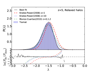
Figure 9: The distribution of Bullock spin parameters for relaxed haloes at redshift 5 in Tiamat. The best fit to Eq 10 centered on $\lambda_{0}=0.033$ and $\alpha=2.25$ is shown as the solid line. Fits from several previous studies are also shown. The lower panel shows the fractional distribution relative to the simulation.

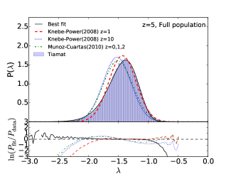
Figure 10: The distribution of Bullock spin parameters for the full sample of haloes in Tiamat at redshift 5, without cutting unrelaxed haloes. The best fit to Eq 10 is centered on $\lambda_{0}=0.042$ and $\alpha=2.70$. Fits from several previous studies are also shown. The lower panel shows the fractional distribution relative to the simulation.

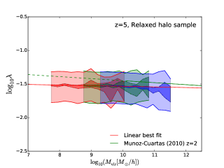
Figure 11: The spin-virial mass relation for relaxed haloes at $z{=}5$. Inner shaded region denotes the bootstrapped 90 per cent confidence interval on the median. The outer shaded region shows the $68$ per cent scatter. The colours red, green and blue represent the Tiny Tiamat, Medi Tiamat and Tiamat simulations. For comparison results for relaxed haloes from Muñoz-Cuartas et al. (2011) are also shown.

Figure 12: The spin-virial mass relation for the full population of haloes at $z{=}5$. Inner shaded region denotes the bootstrapped 90 per cent confidence interval on the median. The outer shaded region shows the $68$ per cent scatter. The colours red, green and blue represent the Tiny Tiamat, Medi Tiamat and Tiamat simulations. For comparison fiducial results for relaxed haloes from Muñoz-Cuartas et al. (2011) are also shown.

5 Discussion and Conclusion

We used N-Body simulations to study concentrations and spins of DM haloes at $z{=}5{-}10$ and across the mass range $10^{8}M_{\odot}h^{-1}<M<10^{11}M_{\odot}h^{-1}$; the regime relevant for studies of structure formation during the epoch of reionization. The dependence of these parameters on equilibrium state was investigated by splitting our halo sample into two populations which include i) only relaxed haloes and ii) the full population. We find qualitatively similar results to previous studies. However, we find quantitative differences between our derived $c({\rm M})$ relations and spin-mass relations and those of previous studies, which we attribute to each author’s use of different halo finders, to our higher simulation resolution, and to the different relaxation criteria used for our sample. We find the model proposed by Ludlow et al. (2014) reproduces both the slope and redshift evolution of our $c({\rm M})$ relation.

Our key results are as follows:

• Our best-fit concentration–mass relations at $z{=}5$ have a slightly negative slope that becomes more shallow towards $z{=}9$. Limiting our analysis to equilibrium haloes has a strong impact on the derived $c({\rm M})$ relation due to unrelaxed haloes having lower concentrations at all masses and redshifts. Haloes with larger center-of-mass offset ($x_{\rm{off}}$) typically have lower concentrations.

• The slope of the $c({\rm M})$ relation becomes shallower at higher redshift, although concentrations decrease at all masses. However, at high redshifts the number of haloes passing the equilibrium criteria is low: only $\sim 30$ per cent of haloes in the 67.8 Mpc$/h$ box pass our resolution and relaxation cuts at $z=5$. Such a high proportion of unrelaxed haloes at the mass scales studied here is a distinct property of the high redshift universe, as discussed in Paper I. We find concentrations of relaxed haloes at $z{>}5$ to be well described by the relation $c_{\rm{vir}}{=}3.2\,({\rm M}/[10^{10}M_{\odot}h^{-1}])^{-0.03}[(1+z)/10]^{-0.29}$ for NFW fits and $c_{\rm{vir}}{=}3.1\,({\rm M}/[10^{10}M_{\odot}h^{-1}])^{-0.03}[(1+z)/10]^{-0.29}$ for Einasto concentrations. The intrinsic scatter around the $c({\rm M})$ relations is $\Delta c_{\rm{vir}}\sim 1$ (or 20 per cent). We find the shape parameter of the Einasto profiles to depend on the peak height mass parameter approximate as $\alpha=0.007\nu^{2}+0.184$.

• Without imposing equilibrium cuts on our sample, the concentrations found in Tiamat have similar values to those reported by Dutton & Macciò (2014), Diemer & Kravtsov (2014) and Hellwing et al. (2015). Concentrations of haloes in Tiamat are a factor of $\Delta c_{\rm{vir}}\sim 0.5-1$ lower than reported by Prada et al. (2012) and Klypin et al. (2014). The shallow negative trend in the $c({\rm M})$ relation that flattens from $z=5$ to $z=10$, and the overall decrease in the magnitude of our Einasto concentrations agree well with Hellwing et al. (2015).

• The distribution of Bullock spin parameters for relaxed haloes at $z{\geq}5$ is found to be well fit by eq. 10 with $(\lambda_{0},\alpha){\sim}(0.033\pm 0.0002,2.25\pm 0.04)$, with little evolution with redshift. Including unrelaxed haloes results in a spin distribution with a higher mean of $\lambda_{0}{=}0.042$.

• As in previous studies, we find a spin-virial mass relation with a slight negative correlation at high redshift. The trend found here has a slope $d\log\lambda/d\log{\rm M}\sim-0.02$ at $z{=}10$. The exclusion of unrelaxed haloes also has the effect of increasing the peak of the spin distribution while the slope of the $\lambda-M_{\rm{vir}}$ relation remains slightly negative. Our best-fit power-law relation relaxed haloes at $z{=}5$ is $\lambda=(0.029\pm 0.004)({\rm M}/[10^{10}M_{\odot}h^{-1}])^{-0.009\pm 0.006}$ and $\lambda=(0.038\pm 0.002)({\rm M}/[10^{10}M_{\odot}h^{-1}])^{-0.009\pm 0.003}$ for the full halo population.

The growth of dark matter haloes drives high-$z$ galaxy formation (Tacchella et al., 2013), while the concentration and spin of haloes are key ingredients for semi-analytic models of galaxy formation (e.g. Croton et al., 2006). This study of these properties for haloes corresponding to the galaxies responsible for reionization will provide a valuable resource for understanding the framework of early galaxy formation.

Acknowledgements This research was supported by the Victorian Life Sciences Computation Initiative (VLSCI), grant ref. UOM0005, on its Peak Computing Facility hosted at the University of Melbourne, an initiative of the Victorian Government, Australia. Part of this work was performed on the gSTAR national facility at Swinburne University of Technology. gSTAR is funded by Swinburne and the Australian Government s Education Investment Fund. This research program is funded by the Australian Research Council through the ARC Laureate Fellowship FL110100072 awarded to JSBW. ADL is financed by a COFUND Junior Research Fellowship. We thank Volker Springel for making the GADGET2 and SUBFIND codes available. We also thank N.Gnedin for useful comments on our manuscript.

References

- Baugh (2006) Baugh C. M., 2006, Reports on Progress in Physics, 69, 3101
- Behroozi et al. (2013) Behroozi P. S., Wechsler R. H., Wu H.-Y., 2013, ApJ, 762, 109
- Bett et al. (2007) Bett P., Eke V., Frenk C. S., Jenkins A., Helly J., Navarro J., 2007, MNRAS, 376, 215
- Bryan & Norman (1998) Bryan G. L., Norman M. L., 1998, ApJ, 495, 80
- Correa et al. (2015) Correa C. A., Wyithe J. S. B., Schaye J., Duffy A. R., 2015, ArXiv e-prints
- Crocce et al. (2006) Crocce M., Pueblas S., Scoccimarro R., 2006, MNRAS, 373, 369
- Croton et al. (2006) Croton D. J. et al., 2006, MNRAS, 365, 11
- Diemer & Kravtsov (2014) Diemer B., Kravtsov A. V., 2014, ArXiv e-prints
- Duffy et al. (2008) Duffy A. R., Schaye J., Kay S. T., Dalla Vecchia C., 2008, MNRAS, 390, L64
- Dutton & Macciò (2014) Dutton A. A., Macciò A. V., 2014, ArXiv e-prints
- Einasto (1965) Einasto J., 1965, Trudy Astrofizicheskogo Instituta Alma-Ata, 5, 87
- Eke et al. (2001) Eke V. R., Navarro J. F., Steinmetz M., 2001, ApJ, 554, 114
- Foreman-Mackey et al. (2013) Foreman-Mackey D., Hogg D. W., Lang D., Goodman J., 2013, PASP, 125, 306
- Gao et al. (2008) Gao L., Navarro J. F., Cole S., Frenk C. S., White S. D. M., Springel V., Jenkins A., Neto A. F., 2008, MNRAS, 387, 536
- Guo et al. (2011) Guo Q. et al., 2011, MNRAS, 413, 101
- Hayashi & White (2008) Hayashi E., White S. D. M., 2008, MNRAS, 388, 2
- Hellwing et al. (2015) Hellwing W. A., Frenk C. S., Cautun M., Bose S., Helly J., Jenkins A., Sawala T., Cytowski M., 2015, ArXiv e-prints
- Kennicutt (1998) Kennicutt, Jr. R. C., 1998, ApJ, 498, 541
- Klypin et al. (2014) Klypin A., Yepes G., Gottlober S., Prada F., Hess S., 2014, ArXiv e-prints
- Klypin et al. (2011) Klypin A. A., Trujillo-Gomez S., Primack J., 2011, ApJ, 740, 102
- Knebe & Power (2008) Knebe A., Power C., 2008, ApJ, 678, 621
- Lagos et al. (2008) Lagos C. D. P., Cora S. A., Padilla N. D., 2008, MNRAS, 388, 587
- Ludlow et al. (2014) Ludlow A. D., Navarro J. F., Angulo R. E., Boylan-Kolchin M., Springel V., Frenk C., White S. D. M., 2014, MNRAS, 441, 378
- Ludlow et al. (2013) Ludlow A. D. et al., 2013, MNRAS, 432, 1103
- Ludlow et al. (2012) Ludlow A. D., Navarro J. F., Li M., Angulo R. E., Boylan-Kolchin M., Bett P. E., 2012, MNRAS, 427, 1322
- Mack (2014) Mack K. J., 2014, MNRAS, 439, 2728
- Meneghetti & Rasia (2013) Meneghetti M., Rasia E., 2013, ArXiv e-prints
- Mo et al. (1998) Mo H. J., Mao S., White S. D. M., 1998, MNRAS, 295, 319
- Muñoz Cuartas et al. (2010) Muñoz Cuartas J. C., Macciò A., Gottlöber S., Dutton A., 2010, in Cosmic Radiation Fields: Sources in the early Universe (CRF 2010), Raue M., Kneiske T., Horns D., Elsaesser D., Hauschildt P., eds., p. 16
- Muñoz-Cuartas et al. (2011) Muñoz-Cuartas J. C., Macciò A. V., Gottlöber S., Dutton A. A., 2011, MNRAS, 411, 584
- Navarro et al. (1997) Navarro J. F., Frenk C. S., White S. D. M., 1997, ApJ, 490, 493
- Navarro et al. (2004) Navarro J. F. et al., 2004, MNRAS, 349, 1039
- Navarro et al. (2010) Navarro J. F. et al., 2010, MNRAS, 402, 21
- Neto et al. (2007) Neto A. F. et al., 2007, MNRAS, 381, 1450
- Planck Collaboration et al. (2015) Planck Collaboration et al., 2015, ArXiv e-prints
- Poole et al. (2015) Poole G. B. et al., 2015, MNRAS, 449, 1454
- Power et al. (2003) Power C., Navarro J. F., Jenkins A., Frenk C. S., White S. D. M., Springel V., Stadel J., Quinn T., 2003, MNRAS, 338, 14
- Prada et al. (2012) Prada F., Klypin A. A., Cuesta A. J., Betancort-Rijo J. E., Primack J., 2012, MNRAS, 423, 3018
- Schmidt (1959) Schmidt M., 1959, ApJ, 129, 243
- Schön et al. (2015) Schön S., Mack K. J., Avram C. A., Wyithe J. S. B., Barberio E., 2015, MNRAS, 451, 2840
- Somerville et al. (2008) Somerville R. S., Hopkins P. F., Cox T. J., Robertson B. E., Hernquist L., 2008, MNRAS, 391, 481
- Springel (2005) Springel V., 2005, MNRAS, 364, 1105
- Springel et al. (2005) Springel V. et al., 2005, Nature, 435, 629
- Springel et al. (2001a) Springel V., White S. D. M., Tormen G., Kauffmann G., 2001a, MNRAS, 328, 726
- Springel et al. (2001b) Springel V., Yoshida N., White S. D. M., 2001b, Nature, 6, 79
- Tacchella et al. (2013) Tacchella S., Trenti M., Carollo C. M., 2013, ApJ, 768, L37
- Wechsler et al. (2002) Wechsler R. H., Bullock J. S., Primack J. R., Kravtsov A. V., Dekel A., 2002, ApJ, 568, 52
- White & Rees (1978) White S. D. M., Rees M. J., 1978, MNRAS, 183, 341
- Zhao et al. (2003) Zhao D. H., Jing Y. P., Mo H. J., Börner G., 2003, ApJ, 597, L9
- Zhao et al. (2009) Zhao D. H., Jing Y. P., Mo H. J., Börner G., 2009, ApJ, 707, 354