Benchmarking sentiment analysis methods for large-scale texts: A case for using continuum-scored words and word shift graphs.

Abstract

The emergence and global adoption of social media has rendered possible the real-time estimation of population-scale sentiment, issuing profound implications for our understanding of human behavior. Given the growing assortment of sentiment measuring instruments, comparisons between them are evidently required. Here, we perform detailed, quantitative tests and qualitative assessments of 6 dictionary-based methods applied to 4 different corpora, and briefly examine a further 20 methods. We show that a dictionary-based method will only perform both reliably and meaningfully if (1) the dictionary covers a sufficiently large enough portion of a given text’s lexicon when weighted by word usage frequency; and (2) words are scored on a continuous scale.

I Introduction

As we move further into what might be called the Sociotechnocene—with increasingly more interactions, decisions, and impact being made by globally distributed people and algorithms—the myriad human social dynamics that have shaped our history have become far more visible and measurable than ever before. Driven by the broad implications of being able to characterize social systems in microscopic detail, sentiment detection for populations at all scale has become a prominent research arena. Attempts to leverage online expression for sentiment mining include prediction of stock markets  bollen2011twitter ; si2013exploiting ; chung2011predicting ; ruiz2012correlating , assessing responses to advertising, real-time monitoring of global happiness dodds2015a , and measuring a health-related quality of life alajajian2015a . The diverse set of instruments produced by this work now provide indicators that help scientists understand collective behavior, inform public policy makers, and in industry, gauge the sentiment of public response to marketing campaigns. Given their widespread usage and potential to influence social systems, understanding how these instruments perform and how they compare with each other has become an imperative. Benchmarking their performance both focuses future development and provides practical advice to non-experts in selecting a dictionary.

We identify sentiment detection methods as belonging to one of three categories, each carrying their own advantages and disadvantages:

1. Dictionary-based methods dodds2015a ; bradley1999a ; pennebaker2001a ; wilson2005a ; liu2010a ; warriner2014a ,

2. Supervised learning methods liu2010a , and

3. Unsupervised (or deep) learning methods socher2013a .

Here, we focus on dictionary-based methods, which all center around the determination of a text $T$’s average happiness (sometimes referred to as valence) through the equation:

$$h_{\textnormal{avg}}(T)=\frac{\sum^{N}_{i=1}h_{\textnormal{avg}}(w_{i})\cdot f_{i}(T)}{\sum^{N}_{i=1}f_{i}(T)}=\sum^{N}_{i=1}h_{\textnormal{avg}}(w_{i})\cdot p_{i}(T),$$ (1)

where we denote each of the $N$ words in a given dictionary as $w_{i}$, word sentiment scores as $h_{\textnormal{avg}}(w_{i})$, word frequency as $f_{i}(T)$, and normalized frequency of $w_{i}$ in $T$ as $p_{i}(T)=f_{i}(T)/\sum^{N}_{i=1}f_{i}(T)$. In this way, we measure the happiness of a text in a manner analogous to taking the temperature of a room. While other simple happiness scores may be considered, we will see that analyzing individual word contributions is important and that this equation allows for a straightforward, meaningful interpretation.

Dictionary-based methods rely upon two distinct advantages we will capitalize on: (1) they are in principle corpus agnostic (including those without training data available) and (2) in contrast to black box (highly non-linear) methods, they offer the ability to “look under the hood” at words contributing to a particular score through “word shifts” (defined fully later; see also  dodds2009b ; dodds2011a ). Indeed, if we are at all concerned with understanding why a particular scoring method varies—e.g,, our undertaking is scientific—then word shifts are essential tools. In the absence of word shifts or similar, any explanation of sentiment trends is missing crucial information and rises only to the level of opinion or guesswork golder2011a ; garcia2015a ; dodds2015b ; wojcik2015conservatives .

As all methods must, dictionary-based “bag-of-words” approaches suffer from various drawbacks, and three are worth stating up front. First, they are only applicable to corpora of sufficient size, well beyond that of a single sentence (widespread usage in this misplaced fashion does not suffice as a counterargument). We directly verify this assertion on individual Tweets, finding that some dictionaries perform admirably, however the average (median) F1-score on the STS-Gold data set is 0.50 (0.54) from all datasets (Table S1), others having shown similar results for dictionary methods with short text ribeiro2016sentibench . Second, state-of-the-art learning methods with a sufficiently large training set for a specific corpus will outperform dictionary-based methods on same corpus liu2012sentiment . However, in practice the domains and topics to which sentiment analysis are applied are highly varied, such that training to a high degree of specificity for a single corpus may not be practical and, from a scientific standpoint, will severely constrain attempts to detect and understand universal patterns. Third: words may be evaluated out of context or with the wrong meaning. A simple example is the word “new” occurring frequently when evaluating articles in the New York Times. This kind of contextual error is something we can readily identify and correct for through word shift graphs, but would remain hidden to nonlinear learning methods without new training.

We lay out our paper as follows. We list and describe the dictionary-based methods we consider in Sec. II, and outline the corpora we use for tests in Sec. II.2. We present our results in Sec. III, comparing all methods in how they perform for specific analyses of the New York Times (NYT) (Sec. III.1), movie reviews (Sec. III.2), Google Books (Sec. III.3), and Twitter (Sec. III.4). In Sec. III.5, we make some basic comparisons between dictionary-based methods and machine learning approaches. We bolster our findings with figures in the Supporting Information, and provide concluding remarks in Sec. IV.

II Dictionaries, Corpora, and Word Shift Graphs

Dictionary	# Fixed	# Stems	Total	Range	# Pos	# Neg	Construction	License	Ref.
labMT	10222	0	10222	1.3 $\to$ 8.5	7152	2977	Survey: MT, 50 ratings	CC	dodds2015a
ANEW	1034	0	1034	1.2 $\to$ 8.8	584	449	Survey: FSU Psych 101	Free for research	bradley1999a
LIWC07	2145	2338	4483	[-1,0,1]	406	500	Manual	Paid, commercial	pennebaker2001a
MPQA	5587	1605	7192	[-1,0,1]	2393	4342	Manual + ML	GNU GPL	wilson2005a
OL	6782	0	6782	[-1,1]	2003	4779	Dictionary propagation	Free	liu2010a
WK	13915	0	13915	1.3 $\to$ 8.5	7761	5945	Survey: MT, at least 14 ratings	CC	warriner2014a
LIWC01	1232	1090	2322	[-1,0,1]	266	344	Manual	Paid, commercial	pennebaker2001a
LIWC15	4071	2478	6549	[-1,0,1]	642	746	Manual	Paid, commercial	pennebaker2001a
PANAS-X	20	0	20	[-1,1]	10	10	Manual	Copyrighted paper	watson1999panas
Pattern	1528	0	1528	-1.0 $\to$ 1.0	575	679	Unspecified	BSD	de2012pattern
SentiWordNet	147700	0	147700	-1.0 $\to$ 1.0	17677	20410	Synset synonyms	CC BY-SA 3.0	baccianella2010sentiwordnet
AFINN	2477	0	2477	[-5,-4, $\ldots$,4,5]	878	1598	Manual	ODbL v1.0	nielsen2011new
GI	3629	0	3629	[-1,1]	1631	1998	Harvard-IV-4	Unspecified	stone1966general
WDAL	8743	0	8743	0.0 $\to$ 3.0	6517	1778	Survey: Columbia students	Unspecified	whissell1986dictionary
EmoLex	14182	0	14182	[-1,0,1]	2231	3243	Survey: MT	Free for research	mohammad2013crowdsourcing
MaxDiff	1515	0	1515	-1.0 $\to$ 1.0	775	726	Survey: MT, MaxDiff	Free for research	kiritchenko2014sentiment
HashtagSent	54129	0	54129	-6.9 $\to$ 7.5	32048	22081	PMI with hashtags	Free for research	zhu2014nrc
Sent140Lex	62468	0	62468	-5.0 $\to$ 5.0	38312	24156	PMI with emoticons	Free for research	MohammadKZ2013
SOCAL	7494	0	7494	-30.2 $\to$ 30.7	3325	4169	Manual	GNU GPL	taboada2011lexicon
SenticNet	30000	0	30000	-1.0 $\to$ 1.0	16715	13285	Label propogation	Citation requested	cambria2014senticnet
Emoticons	132	0	132	[-1,0,1]	58	48	Manual	Open source code	gonccalves2013comparing
SentiStrength	1270	1345	2615	[-5,-4, $\ldots$,4,5]	601	2002	LIWC+GI	Unknown	thelwall2010sentiment
VADER	7502	0	7502	-3.9 $\to$ 3.4	3333	4169	MT survey, 10 ratings	Freely available	hutto2014vader
Umigon	927	0	927	[-1,1]	334	593	Manual	Public Domain	levallois2013umigon
USent	592	0	592	[-1,1]	63	529	Manual	CC	pappas2013distinguishing
EmoSenticNet	13188	0	13188	[-10,-2,-1,0,1,10]	9332	1480	Bootstrapped extension	Non-commercial	poria2013enhanced

Table 1: Summary of dictionary attributes used in sentiment measurement instruments. We provide all acronyms and abbreviations and further information regarding dictionaries in Sec. II.1. We test the first 6 dictionaries extensively. # Fixed, # Stems, # Pos and # Neg refer to the numbers of: terms in the dictionary that are fixed words, stems used to match words, terms that are rated above neutral, and terms rated below neutral. The range indicates whether scores are continuous or binary (we use the term binary for dictionaries for which words are scored as $\pm 1$ and optionally 0).

II.1 Dictionaries

The words “dictionary,” “lexicon,” and “corpus” are often used interchangeably, and for clarity we define our usage as follows.

Dictionary:

Set of words (possibly including word stems) with ratings.

Corpus:

Collection of texts which we seek to analyze.

Lexicon:

The words contained within a corpus (often said to be “tokenized”).

We test the following six dictionaries in depth:

labMT

— language assessment by Mechanical Turk dodds2015a .

ANEW

— Affective Norms of English Words bradley1999a .

WK

— Warriner and Kuperman rated words from SUBTLEX by Mechanical Turk warriner2014a .

MPQA

— The Multi-Perspective Question Answering (MPQA) Subjectivity Dictionary wilson2005a .

LIWC{01,07,15}

— Linguistic Inquiry and Word Count, three versions pennebaker2001a .

OL

— Opinion Lexicon, developed by Bing Liu liu2010a .

We also make note of 18 other dictionaries:

PANAS-X

— The Positive and Negative Affect Schedule — Expanded watson1999panas .

Pattern

— A web mining module for the Python programming language, version 2.6 de2012pattern .

SentiWordNet

— WordNet synsets each assigned three sentiment scores: positivity, negativity, and objectivity baccianella2010sentiwordnet .

AFINN

— Words manually rated -5 to 5 with impact scores by Finn Nielsen nielsen2011new .

GI

— General Inquirer: database of words and manually created semantic and cognitive categories, including positive and negative connotations stone1966general .

WDAL

— Whissel’s Dictionary of Affective Language: words rated in terms of their Pleasantness, Activation, and Imagery (concreteness) whissell1986dictionary .

EmoLex

— NRC Word-Emotion Association Lexicon: emotions and sentiment evoked by common words and phrases using Mechanical Turk mohammad2013crowdsourcing .

MaxDiff

— NRC MaxDiff Twitter Sentiment Lexicon: crowdsourced real-valued scores using the MaxDiff method kiritchenko2014sentiment .

HashtagSent

— NRC Hashtag Sentiment Lexicon: created from tweets using Pairwise Mutual Information with sentiment hashtags as positive and negative labels (here we use only the unigrams) zhu2014nrc .

Sent140Lex

— NRC Sentiment140 Lexicon: created from the “sentiment140” corpus of tweets, using Pairwise Mutual Information with emoticons as positive and negative labels (here we use only the unigrams) MohammadKZ2013 .

SOCAL

— Manually constructed general-purpose sentiment dictionary taboada2011lexicon .

SenticNet

— Sentiment dataset labeled with semantics and 5 dimensions of emotions by Cambria et al., version 3 cambria2014senticnet .

Emoticons

— Commonly used emoticons with their positive, negative, or neutral emotion gonccalves2013comparing .

SentiStrength

— an API and Java program for general purpose sentiment detection (here we use only the sentiment dictionary) thelwall2010sentiment .

VADER

— method developed specifically for Twitter and social media analysis hutto2014vader .

Umigon

— Manually built specifically to analyze Tweets from the sentiment140 corpus levallois2013umigon .

USent

— set of emoticons and bad words that extend MPQA pappas2013distinguishing .

EmoSenticNet

— extends SenticNet words with WNA labels poria2013enhanced .

All of these dictionaries were produced by academic groups, and with the exception of LIWC, they are provided free of charge. In Table 1, we supply the main aspects—such as word count, score type (continuum or binary), and license information—for the dictionaries listed above. In the github repository associated with our paper, https://github.com/andyreagan/sentiment-analysis-comparison, we include all of the dictionaries but LIWC.

The LabMT, ANEW, and WK dictionaries have scores ranging on a continuum from 1 (low happiness) to 9 (high happiness) with 5 as neutral, whereas the others we test in detail have scores of $\pm 1$, and either explicitly or implicitly 0 (neutral). We will refer to the latter dictionaries as being binary, even if neutral is included. Other non-binary ranges include a continuous scale from -1 to 1 (SentiWordNet), integers from -5 to 5 (AFINN), continuous from 1 to 3 (GI), and continuous from -5 to 5 (NRC). For coverage tests, we include all available words, to gain a full sense of the breadth of each dictionary. In scoring, we do not include neutral words from any dictionary.

We test the LabMT, ANEW, and WK dictionaries for a range of stop words (starting with the removal of words scoring within $\Delta_{h}=1$ of the neutral score of 5) dodds2011a . The ability to remove stop words is one advantage of dictionaries that have a range of scores, allowing us to tune the instrument for maximum performance, while retaining all of the benefits of a dictionary method. We will show that, in agreement with the original paper introducing LabMT and looking at Twitter data, a $\Delta_{h}=1$ is a pragmatic choice in general dodds2011a .

Since we do not apply a part of speech tagger, when using the MPQA dictionary we are obliged to exclude words with scores of both +1 and -1. The words and stems with both scores are: blood, boast* (we denote stems with an asterisk), conscience, deep, destiny, keen, large, and precious. We choose to match a text’s words using the fixed word set from each dictionary before stems, hence words with overlapping matches (a fixed word that also matches a stem) are first matched by the fixed word.

II.2 Corpora Tested

For each dictionary, we test both the coverage and the ability to detect previously observed and/or known patterns within each of the following corpora, noting the pattern we hope to discern:

1. The New York Times (NYT) nytimescorpus2008a : Goal of ranking sections by sentiment (Sec. III.1).

2. Movie reviews pang2004a : Goal of discerning positive and negative reviews (Sec. III.2).

3. Google Books lin2012syntactic : Goal of creating time series (Sec. III.3).

4. Twitter: Goal of creating time series (Sec. III.4).

For the corpora other than the movie reviews and small numbers of tagged Tweets, there is no publicly available ground truth sentiment, so we instead make comparisons between methods and examine how words contribute to scores. We note that comparison to societal measures of well being would also be possible Mitchell2013a . We offer greater detail on corpus processing below, and we also provide the relevant scripts on github at https://github.com/andyreagan/sentiment-analysis-comparison.

II.3 Word Shift Graphs

Sentiment analysis is applied in many circumstances in which the goal of the analysis goes beyond simply categorizing text into positive or negative. Indeed if this were the only use case, the value added by sentiment analysis would be severely limited. Instead we use sentiment analysis methods as a lens that allow us to see how the emotive words in a text shape the overall content. This is accomplished by analyzing each word for the individual contribution to the sentiment score (or to the difference in the sentiment score between two texts). In either case, we need to consider the words ranked by this individual contribution.

Of the four corpora that we use as benchmarks, three rely on this type of qualitative analysis: using the dictionary as a tool to better understand the sentiment of the corpora. For this case, we must first find the contribution of each word individually. Starting with two texts, we take the difference of their sentiment scores, rearrange a few things, and arrive at

$$h^{\textrm{(comp)}}_{\textrm{avg}}-h^{\textrm{(ref)}}_{\textrm{avg}}=\sum_{w\in L}\underbrace{\left[h_{\textrm{avg}}{(w)}-h^{\textrm{(ref)}}_{\textrm{avg}}\right]}_{+/-}\underbrace{\left[p_{w}^{\textrm{(comp)}}-p_{w}^{\textrm{(ref)}}\right]}_{\uparrow/\downarrow}.$$

Each word contributes to the word shift according to its happiness relative to the reference text ($+/-$ = more/less emotive), and its change in frequency of usage ($\uparrow/\downarrow$ = more/less frequent). As a first step, it is possible to visualize this sorted word list in a table, along with the basic indicators of how its contribution is constituted. We use word shift graphs to present this information in the most accessible manner to advanced users.

For further detail, we refer the reader to our instructional post and video at http://www.uvm.edu/storylab/2014/10/06/.

III Results

In Fig 1, we show a direct comparison between word scores for each pair of the 6 dictionaries tested. Overall, we find strong agreement between all dictionaries with exceptions we note below. As a guide, we will provide more detail on the individual comparison between the LabMT dictionary and the other five dictionaries by examining the words whose scores disagree across dictionaries shown in Fig 2. We refer the reader to the S2 Appendix for the remaining individual comparisons.

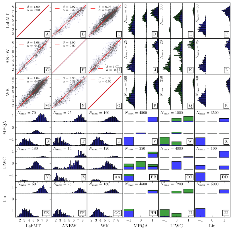
Figure 1: Direct comparison of the words in each of the dictionaries tested. For the comparison of two dictionaries, we plot words that are matched by the independent variable “$x$” in the dependent variable “$y$”. Because of this, and cross stem matching, the plots are not symmetric across the diagonal of the entire figure. Where the scores are continuous in both dictionaries, we compute the RMA linear fit. When a dictionary contains both fixed and stem words, we plot the matches by fixed words in blue and by stem words in green. The axes in the bar plots are not of the same height, due to large mismatches in the number of words in the dictionaries, and we note the maximum height of the bar in the upper left of such plots. Detailed analysis of Panel C can be found in dodds2015b . We provide a table for each off-diagonal panel in the S2 Appendix with the words whose scores exhibit the greatest mismatch, and a subset of these tables in Fig 2.

To start with, consider the comparison the LabMT and ANEW on a word for word basis. Because these dictionaries share the same range of values, a scatterplot is the natural way to visualize the comparison. Across the top row of Fig 1, which compares LabMT to the other 5 dictionaries, we see in Panel B for the LabMT-ANEW comparison that the RMA best fit rayner1985a is

$$h_{w_{\textnormal{LabMT}}}=0.92*h_{w_{\textnormal{ANEW}}}+0.40$$

for words $w_{\textnormal{LabMT}}$ in LabMT and words $w_{\textnormal{ANEW}}$ in ANEW. The 10 words with farthest from the line of best fit shown in Panel B of Fig 2 are, with LabMT and ANEW scores: lust (4.64, 7.12), bees (5.60, 3.20), silly (5.30, 7.41), engaged (6.16, 8.00), book (7.24, 5.72), hospital (3.50, 5.04), evil (1.90, 3.23), gloom (3.56, 1.88), anxious (3.42, 4.81), and flower (7.88, 6.64). These are words whose individual ranges have high standard deviations in LabMT. While the overall agreement is very good, we should expect some variation in the emotional associations of words, due to chance, time of survey, and demographic variability. Indeed, the Mechanical Turk users who scored the words for the LabMT set in 2011 are evidently different from the University of Florida students who took the ANEW survey before 2000 as a class requirement for Introductory Psychology.

Comparing LabMT with WK in Panel C of Fig 1, we again find a fit with slope near 1, and a smaller positive shift: $h_{w_{\textnormal{LabMT}}}=0.96*h_{w_{\textnormal{WK}}}+0.26$. The 10 words farthest from this line, shown in Panel B of Fig 2, are (LabMT, WK): sue (4.30, 2.18), boogie (5.86, 3.80), exclusive (6.48, 4.50), wake (4.72, 6.57), federal (4.94, 3.06), stroke (2.58, 4.19), gay (4.44, 6.11), patient (5.04, 6.71), user (5.48, 3.67), and blow (4.48, 6.10). Like LabMT, the WK dictionary used a Mechanical Turk online survey to gather word ratings. We speculate that the minor variation is due in part to the low number of scores required for each word in the WK survey, with as few as 14 ratings per words and 18 ratings for the majority of the words. By contrast, LabMT scores represent 50 ratings of each word. For an in depth comparison, see reference dodds2015b .

Next, in comparing binary dictionaries with $\pm 1$ or $\pm 1,0$ scores to one with a 1–9 range, we can look at the distribution of scores within the continuum score dictionary for each score in the binary dictionary. Looking at the LabMT-MPQA comparison in Panel D of Fig 1, we see that most of the matches are between words without stems (blue histograms), and that each score in -1, 0, +1 from MPQA corresponds to a distribution of scores in LabMT. To examine deviations, we take the words from LabMT sorted by happiest when MPQA is -1, both the happiest and the least happy when MPQA is 0, and the least happy when MPQA is 1 (Fig 2 Panels C-E). The 10 happiest words in LabMT matched by MPQA words with score -1 are: moonlight (7.50), cutest (7.62), finest (7.66), funniest (7.76), comedy (7.98), laughs (8.18), laughing (8.20), laugh (8.22), laughed (8.26), laughter (8.50). This is an immediately troubling list of evidently positive words somehow rated as -1 in MPQA. We also see that the top 5 are matched by the stem “laugh*” in MPQA. The least happy 5 words and happiest 5 words in LabMT matched by words in MPQA with score 0 are: sorrows (2.69), screaming (2.96), couldn’t (3.32), pressures (3.49), couldnt (3.58), and baby (7.28), precious (7.34), strength (7.40), surprise (7.42), song (7.58). Again, we see MPQA word scores are questionable. The least happy words in LabMT with score +1 in MPQA that are matched by MPQA are: vulnerable (3.34), court (3.78), sanctions (3.86), defendant (3.90), conviction (4.10), backwards (4.22), courts (4.24), defendants (4.26), court’s (4.44), and correction (4.44). Clearly, these words are not positive words in most contexts.

While it would be simple to correct these ratings in the MPQA dictionary going forward, we have are naturally led to be concerned about existing work using MPQA. We note again that the use of word shifts of some kind would have exposed these problematic scores immediately.

Figure 2: We present the specific words from Panels G, M, S and Y of Fig 1 with the greatest mismatch. Only the center histogram from Panel Y of Fig 1 is included. We emphasize that the LabMT dictionary scores generally agree well with the other dictionaries, and we are looking at the marginal words with the strongest disagreement. Within these words, we detect differences in the creation of these dictionaries that carry through to these edge cases. Panel A: The words with most different scores between the LabMT and ANEW dictionaries are suggestive of the different meanings that such words entail for the different demographic surveyed to score the words. Panel B: Both dictionaries use surveys from the same demographic (Mechanical Turk), where the LabMT dictionary required more individual ratings for each word (at least 50, compared to 14) and appears to have dampened the effect of multiple meaning words. Panels C–E: The words in LabMT matched by MPQA with scores of -1, 0, and +1 in MPQA show that there are at least a few words with negative rating in MPQA that are not negative (including the happiest word in the LabMT dictionary: “laughter”), not all of the MPQA words with score 0 are neutral, and that MPQA’s positive words are mostly positive according to the LabMT score. Panel F: The function words in the expert-curated LIWC dictionary are not emotionally neutral.

For the LabMT-LIWC comparison in Panel E of Fig 1 we examine the same matched word lists as before. The 10 happiest words in LabMT matched by words in LIWC with score -1 are: trick (5.22), shakin (5.29), number (5.30), geek (5.34), tricks (5.38), defence (5.39), dwell (5.47), doubtless (5.92), numbers (6.04), shakespeare (6.88). From Panel F of Fig 2, the least happy 5 neutral words and happiest 5 neutral words in LIWC, matched with LIWC, are: negative (2.42), lack (3.16), couldn’t (3.32), cannot (3.32), never (3.34), millions (7.26), couple (7.30), million (7.38), billion (7.56), millionaire (7.62). The least happy words in LabMT with score +1 in LIWC that are matched by LIWC are: merrill (4.90), richardson (5.02), dynamite (5.04), careful (5.10), richard (5.26), silly (5.30), gloria (5.36), securities (5.38), boldface (5.40), treasury’s (5.42). The +1 and -1 words in LIWC match some neutral words in LabMT, which is not alarming. However, the problems with the “neutral” words in the LIWC set are immediate: these are not emotionally neutral words. The range of scores in LabMT for these 0-score words in LIWC formed the basis for Garcia et al.’s response to dodds2015a , and we point out here that the authors must have not looked at the words, and all-too-common problem in studies using sentiment analysis garcia2015a ; dodds2015b .

For the LabMT-OL comparison in Panel E of Fig 1 we again examine the same matched word lists as before, except the neutral word list because OL has no explicit neutral words. The 10 happiest words in LabMT matched by OL’s negative list are: myth (5.90), puppet (5.90), skinny (5.92), jam (6.02), challenging (6.10), fiction (6.16), lemon (6.16), tenderness (7.06), joke (7.62), funny (7.92). The least happy words in LabMT with score +1 in OL that are matched by OL are: defeated (2.74), defeat (3.20), envy (3.33), obsession (3.74), tough (3.96), dominated (4.04), unreal (4.57), striking (4.70), sharp (4.84), sensitive (4.86). Despite nearly twice as many negative words in OL as positive words (at odds with the frequency-dependent positivity bias of language dodds2015a ), these dictionaries generally agree.

III.1 New York Times Word Shift Analysis

The New York Times corpus nytimescorpus2008a is split into 24 sections of the newspaper that are roughly contiguous throughout the data from 1987–2008. With each dictionary, we rate each section and then compute word shifts (described below) against the baseline, and produce a happiness ranked list of the sections. In the first Figure in S4 Appendix we show scatterplots for each comparison, and compute the Reduced Major Axes (RMA) regression fit rayner1985a . In the second Figure in S4 Appendix we show the sorted bar chart from each dictionary.

To gain understanding of the sentiment expressed by any given text relative to another text, it is necessary to inspect the words which contribute most significantly by their emotional strength and the change in frequency of usage. We do this through the use of word shift graphs, which plot the contribution of each word $w_{i}$ from the dictionary (denoted $\delta h_{\textnormal{avg}}(w_{i})$) to the shift in average happiness between two texts, sorted by the absolute value of the contribution. We use word shift graphs to both analyze a single text and to compare two texts, here focusing on comparing text within corpora. For a derivation of the algorithm used to make word shift graphs while separating the frequency and sentiment information, we refer the reader to Equations 2 and 3 in dodds2011a . We consider both the sentiment difference and frequency difference parts of $\delta h_{\textnormal{avg}}(w_{i})$ by writing each term of Eq. 1 as in dodds2011a :

$$\delta h_{\textnormal{avg}}(w_{i})=\\ 100\frac{h_{\textnormal{avg}}(w_{i})-h_{\textnormal{avg}}(T_{\textnormal{ref}})}{h_{\textnormal{avg}}(T_{\textnormal{comp}})-h_{\textnormal{avg}}(T_{\textnormal{ref}})}\left[p_{i}(T_{\textnormal{comp}})-p_{i}(T_{\textnormal{ref}})\right].$$ (2)

An in-depth explanation of how to interpret the word shift graph can also be found at http://hedonometer.org/instructions.html#wordshifts.

To both demonstrate the necessity of using word shift graphs in carrying out sentiment analysis, and to gain understanding about the ranking of New York Times sections by each dictionary, we look at word shifts for the “Society” section of the newspaper from each dictionary in Fig 3, with the reference text being the whole of the New York Times. The “Society” section happiness ranks 1, 1, 1, 18, 1, and 11 within the happiness of each of the 24 sections in the dictionaries LabMT, ANEW, WK, MPQA, LIWC, and OL, respectively. These shifts show only the very top of the distributions which range in length from 1030 (ANEW) to 13915 words (WK).

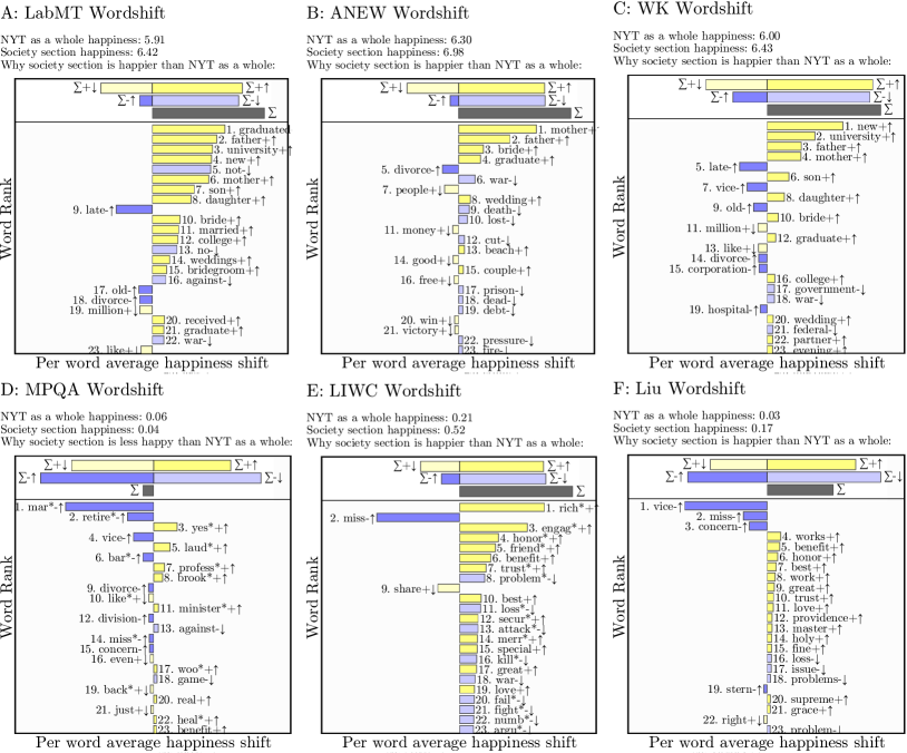
Figure 3: New York Times (NYT) “Society” section shifted against the entire NYT corpus for each of the six dictionaries listed in tiles A–F. We provide a detailed analysis in Sec. III.1. Generally, we are able to glean the greatest understanding of the sentiment texture associated with this NYT section using the LabMT dictionary. Additionally we note the LabMT dictionary has the most coverage quantified by word match count (Figure in S3 Appendix), we are able to identify and correct problematic words scores in the OL dictionary, and we see that the MPQA dictionary disagrees entirely with the others because of an overly broad stem match.

First, using the LabMT dictionary, we see that the words 1. “graduated”, 2. “father”, and 3. “university” top the list, which is dominated by positive words that occur more frequently. These more frequent positive words paint a clear picture of family life (relationships, weddings, and divorces), as well as university accomplishment (graduations and college). In general, we are able to observe with only these words that the “Society” section is where we find the details of these positive events.

From the ANEW dictionary, we see that a few positive words are up, lead by 1. “mother”, 2. “father”, and 3. “bride”. Looking at this shift in isolation, we see only these words with three more (“graduate”, “wedding”, and “couple”) that would lead us to suspect these events are at least common in the “Society” section.

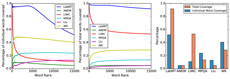
Figure S3: Coverage of the words in the New York Times by each of the dictionaries.

The WK dictionary, with the most individual word scores of any dictionary tested, agrees with LabMT and ANEW that the “Society” section is number 1, with somewhat similar set of words at the top: 1. “new”, 2. “university”, and 3. “father”. Less coverage of the New York Times corpus (see Fig S3) results in the top of the shift showing less of the character of the “Society” section than LabMT, with more words that go down in frequency in the shift. With the words “bride” and “wedding” up, as well as “university”, “graduate”, and “college”, we glean that the “Society” section covers both graduations and weddings, as we have seen so far.

The MPQA dictionary ranks the “Society” section 18th of the 24 NYT sections, a complete departure from the other rankings, with the words 1. “mar*”, 2. “retire*”, and 3. “yes*” the top three contributing words. Negative words increasing in frequency are the most common type near the top, and of these, the words with the biggest contributions are being scored incorrectly in this context (specifically words 1. “mar*”, 2. “retire*”, 6. “bar*”, 12. “division”, and 14. “miss*”). Looking more in depth at the problems created by the first of these, we find 1211 unique words match “mar*” with the five most frequent being married (36750), marriage (5977), marketing (5382), mary (4403), and mark (2624). The score for these words in, for example, LabMT are 6.76, 6.7, 5.2, 5.88, and 5.48, confirming our suspicion about these words being categorized incorrectly with a broad stem match. These problems plague the MPQA dictionary for scoring the New York Times corpus, and without using word shifts would have gone completely unseen. In an attempt to fix contextual issues by blocking corpus-specific words, we block “mar*,retire*,vice,bar*,miss*” and find that the MPQA dictionary ranks the Society section of the NYT at 15th of the 24 sections

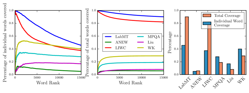
Figure 4: Coverage of the words in the movie reviews by each of the dictionaries. We observe that the LabMT dictionary has the highest coverage of words in the movie reviews corpus both across word rank and cumulatively. The LIWC dictionary has initially high coverage since it contains some high-frequency function words, but quickly drops off across rank. The WK dictionary coverage increases across word rank and cumulatively, indicating that it contains a large number of less common words in the movie review corpus. The OL, ANEW, and MPQA have a cumulative coverage of less than 20% of the lexicon.

The second $\pm 1$ dictionary, LIWC, agrees well with the first three dictionaries and places the “Society” section at the top with the words 1. “rich*”, 2. “miss”, and 3. “engage*” at the head of the list. We immediately notice that the word “miss” is being used frequently in the “Society” section in a different context than was rated LIWC: it is used in the corpus to mean the title prefixed to the name of an unmarried woman, but is scored as negative in LIWC as meaning to fail to reach an target or to acknowledge loss. We would remove this word from LIWC for further analysis of this corpus (we would also remove the word “trust” here). The words matched by “miss*” aside, LIWC finds some positive words going up, with “engage*” hinting at weddings. Otherwise, without words that capture the specific behavior happening in the “Society” section, we are unable to see anything about college, graduations, or marriages, and there is much less to be gained about the text from the words in LIWC than some of the other dictionaries we have seen. Without these words, it is confirming that LIWC still finds the “Society” section to be the top section, due in large part to a lack of negative words 18. “war” and 21. “fight*”.

The final dictionary from OL disagrees with the others and puts the “Society” section at 11th out of the 24 sections. The top three words, 1. “vice”, 2. “miss”, and 3. “concern”, contribute largely with respect to the rest of distribution, of which two are clearly being used in an inappropriate context. For a more reasonable analysis we would remove both “vice” and “miss” from the OL dictionary to score this text, making the “Society” section the second happiest of the 24 sections. With this fix, the OL dictionary ranks the Society section of the NYT as the happiest section. Focusing on the words, we see that the OL dictionary finds many positive words increasing in frequency that are mostly generic. In the word shift we do not find the wedding or university events as in dictionaries with more coverage, but rather a variety of positive language surrounding these events, for example 4. “works”, 5. “benefit”, 6. “honor”, 7. “best”, 9. “great”, 10. “trust”, 11. “love”, etc.

In conclusion, we find that 4 of the 6 dictionaries score the “Society” section at number 1, and in these cases we use the word shift to uncover the nuances of the language used. We find, unsurprisingly, that the most matches are found by the LabMT dictionary, which is in part built from the NYT corpus (see S3 Appendix for coverage plots). Without as much corpus-specific coverage, we note that while the nuances of the text remain hidden, the LIWC and OL dictionaries still find the positivity surrounding these unknown events. Of the two that did not score the “Society” section at the top, we repair the MPQA and the OL dictionaries by removing the words “mar*,retire*,vice*,bar*,miss*” and “vice,miss”, respectively. By identifying words used in the wrong context using the word shift graph, we directly improve the sentiment score for the New York Times corpus from both MPQA and OL dictionaries. While the OL dictionary, with two corrections, agrees with the other dictionaries, the MPQA dictionary with five corrections still ranks the Society section of the NYT as the 15th happiest of the 24 sections.

III.2 Movie Reviews Classification and Word Shift Analysis

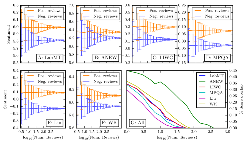
Figure 5: The score assigned to increasing numbers of reviews drawn from the tagged positive and negative sets. For each dictionary we show mean sentiment and 1 standard deviation over 100 samples for each distribution of reviews in Panels A–F. For comparison we compute the fraction of the distributions that overlap in Panel G. At the single review level for each dictionary this simple performance statistic (fraction of distribution overlap) ranks the OL dictionary in first place, the MPQA, LIWC, and LabMT dictionaries in a second place tie, WK in fifth, and ANEW far behind. All dictionaries require on the order of 1000 words to achieve 95% classification accuracy.

For the movie reviews, we test the ability to discern positive and negative reviews. The entire dataset consists of 1000 positive and 1000 negative reviews, as rated with 4 or 5 stars and 1 or 2 stars, respectively. We show how well each dictionary covers the review database in Fig 4. The average review length is 650 words, and we plot the distribution We average the sentiment of words in each review individually, using each dictionary. We also combine random samples of $N$ positive or $N$ negative reviews for $N$ varying from 2 to 900 on a logarithmic scale, without replacement, and rate the combined text. With an increase in the size of the text, we expect that the dictionaries will be better able to distinguish positive from negative. The simple statistic we use to describe this ability is the percentage of distributions that overlap the average.

In the lower right panel of Fig 5, the percentage overlap of positive and negative review distributions presents us with a simple summary of dictionary performance on this tagged corpus. The ANEW dictionary stands out as being considerably less capable of distinguishing positive from negative. In order, we then see WK is slightly better overall, LabMT and LIWC perform similarly better than WK overall, and then MPQA and OL are each a degree better again, across the review lengths (see below for hard numbers at 1 review length). Two Figures in S5 Appendix show the distributions for 1 review and for 15 combined reviews.

To analyze which words are being used by each dictionary, we compute word shift graphs of the entire positive corpus versus the entire negative corpus in Fig 6. Across the board, we see that a decrease in negative words is the most important word type for each dictionary, with the word “bad” being the top word for every dictionary in which it is scored (ANEW does not have it). Other observations that we can make from the word shifts include a few words that are potentially being used out of context: “movie”, “comedy”, “plot”, “horror”, “war”, “just”.

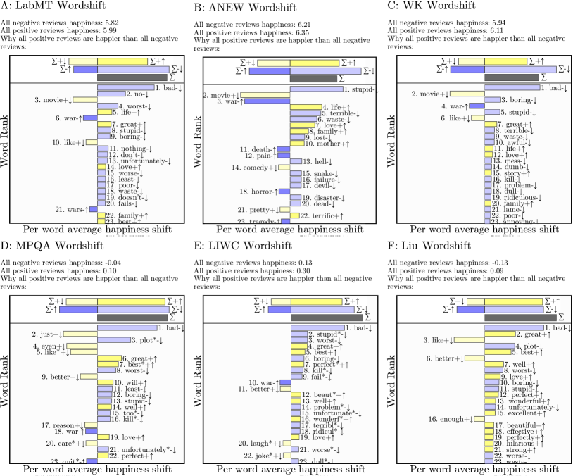
Figure 6: Word shifts for the movie review corpus. By analyzing the words that contribute most significantly to the sentiment score produced by each dictionary we are able to identify words that are problematic for each dictionary at the word-level, and generate an understanding of the emotional texture of the movie review corpus. Again we find that coverage of the lexicon is essential to produce meaningful word shifts, with the LabMT dictionary providing the most coverage of this corpus and producing the most detailed word shifts. All words on the left hand side of these word shifts are words that individually made the positive reviews score more negatively than the negative reviews, and the removal of these words would improve the accuracy of the ratings given by each dictionary. In particular, across each dictionary the word shifts show that domain-specific words such as “war” and “movie” are used more frequently in the positive reviews and are not useful in determining the polarity of a single review.

Classifying single reviews as positive or negative, the F1-scores are: LabMT .63, ANEW .36, LIWC .53, MPQA .66, OL .71, and WK .34 (see Table S4). We roughly confirm the rule-of-thumb that 10,000 words are enough to score with a dictionary confidently, with all dictionaries except MPQA and ANEW achieving 90% accuracy with this many words. We sample the number of reviews evenly in log space, generating sets of reviews with average word counts of 4550, 6500, 9750, 16250, and 26000 words. Specifically, the number of reviews necessary to achieve 90% accuracy is 15 reviews (9750 words) for LabMT, 100 reviews (65000 words) for ANEW, 10 reviews (6500 words) for LIWC, 10 reviews (6500 words) for MPQA, 7 reviews (4550 words) for OL, and 25 reviews (16250 words) for WK.

The OL dictionary, with the highest performance classifying individual movie reviews of the 6 dictionaries tested in detail, performs worse than guessing at classifying individual sentences in movie reviews. Specifically, 76.9/74.2% of sentences in the positive/negative reviews sets have words in the OL dictionary, and of these OL achieves an F1-score of 0.44. The results for each dictionary are included in Table S5, with an average (median) F1 score of 0.42 (0.45) across all dictionaries.

III.3 Google Books Time Series and Word Shift Analysis

We use the Google books 2012 dataset with all English books lin2012syntactic , from which we remove part of speech tagging and split into years. From this, we make time series by year, and word shifts of decades versus the baseline. In addition, to assess the similarity of each time series, we produce correlations between each of the time series.

Despite grand claims from research based on the Google Books corpus michel2011quantitative , we keep in mind that there are several deep problems with this beguiling data set pechenick2015a . Leaving aside these issues, the Google Books corpus nevertheless provides a substantive test of our six dictionaries.

In Fig 7, we plot the sentiment time series for Google Books. Three immediate trends stand out: a dip near the Great Depression, a dip near World War II, and a general upswing in the 1990’s and 2000’s. From these general trends, a few dictionaries waver: OL does not dip very much for WW2, OL and LIWC stay lower in the 90’s and 2000’s, and LabMT with $\Delta_{h}=0.5,1.0$ go downward near the end of the 2000’s. We take a closer look into the 1940’s to see what each dictionary is picking up in Google Books around World War 2 in Figure in S6 Appendix.

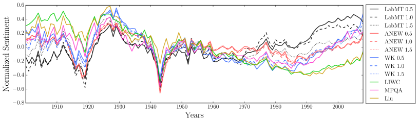
Figure 7: Google Books sentiment time series from each dictionary, with stop values of 0.5, 1.0, and 1.5 from the dictionaries with word scores in the 1–9 range. To normalize the sentiment score, we subtract the mean and divide by the absolute range. We observe that each time series is choppy, with a few pronounced negative time periods, and trending positive towards the end of the corpus. The score of LabMT varies substantially with different stop values, although remaining highly correlated, and finds absolute lows near the World Wars. The LIWC and OL dictionaries trend down towards 1990, dipping as low as the war periods.

In each panel of the word shift Figure in S6 Appendix, we see that the top word making the 1940’s less positive than the the rest of Google Books is “war”, which is the top contributor for every dictionary except OL. Rounding out the top three contributing words are “no” and “great”, and we infer that the word “great” is being seen from mention of “The Great Depression” or “The Great War”, and is possibly being used out of context. All dictionaries but ANEW have “great” in the top 3 words, and each dictionary could be made more accurate if we remove this word.

In Panel A of the 1940’s word shift Figure in S6 Appendix, beyond the top words, increasing words are mostly negative and war-related: “against”, “enemy”, “operation”, which we could expect from this time period.

In Panel B, the ANEW dictionary scores the 1940’s of Google Books lower than the baseline as well, finding “war”, “cancer”, and “cell” to be the most important three words. With only 1030 words, there is not enough coverage to see anything beyond the top word “war,” and the shift is dominated by words that go down in frequency.

In Panel C, the WK dictionary finds the the 1940’s with slightly less happy than the baseline, with the top three words being “war”, “great”, and “old”. We see many of the same war-related words as in LabMT, and in addition some positive words like “good” and “be” are up in frequency. The word “first” could be an artifact of first aid.

In Panel D, the MPQA dictionary rates the 1940’s with slightly less happy than the baseline, with the top three words being “war”, “great”, and “differ*”. Beyond the top word “war”, the score is dominated by words decreasing in frequency, with only a few words up in frequency. Without specific words being up in frequency, it is difficult to obtain a good glance at the nature of the text here.

In Panel E, the LIWC dictionary rates the 1940’s nearly the same as the baseline, with the top three words being “war”, “great”, and “argu*”. When the scores are nearly the same, although the 1940’s are slightly higher happiness here, the word shift is a view into how the words of the reference and comparison text vary. In addition to a few war related words being up and bringing the score down (“fight”, “enemy”, “attack”), we see some positive words up that could also be war related: “certain”, “interest”, and “definite”. Although LIWC does not manage to find World War II as a low point of the 20th century, the words that it generates are useful in understanding the corpus.

In Panel F, the OL dictionary rates the 1940’s as happier than the baseline, with the top three words being “great”, “support”, and “like”. With 7 positive words up, and 1 negative word up, we see how the OL dictionary misses the war without the word “war” itself and with only “enemy” contributing from the words surrounding the conflict. The nature of the positive words that are up is unclear, and could justify a more detailed analysis of why the OL dictionary fails here.

III.4 Twitter Time Series Analysis

We store data on the Vermont Advanced Computing Core (VACC), and process the text first into hash tables (with approximately 8 million unique English words each day) and then into word vectors for each 15 minutes, for each dictionary tested. From this, we build sentiment time series for time resolutions of 15 minutes, 1 hour, 3 hours, 12 hours, and 1 day. In addition to the raw time series, we compute correlations between each time series to assess the similarity of the ratings between dictionaries.

In Fig 8, we present a daily sentiment time series of Twitter processed using each of the dictionaries being tested. With the exception of LIWC and MPQA we observe that the dictionaries generally track well together across the entire range. A strong weekly cycle is present in all, although muted for ANEW.

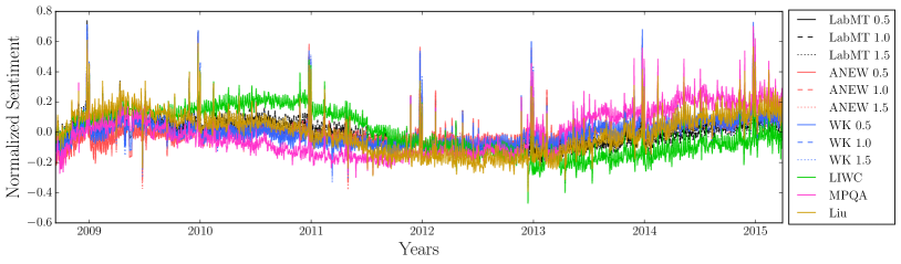
Figure 8: Normalized sentiment time series on Twitter using $\Delta_{h}$ of 1.0 for all dictionaries. To normalize the sentiment score, we subtract the mean and divide by the absolute range. The resolution is 1 day, and draws on the 10% gardenhose sample of public tweets provided by Twitter. All of the dictionaries exhibit wide variation for very early Tweets, and from 2012 onward generally track together strongly with the exception of MPQA and LIWC. The LIWC and MPQA dictionaries show opposite trends: a rise until 2012 with a decline after 2012 from LIWC, and a decline before 2012 with a rise afterwards from MPQA. To analyze the trends we look at the words driving the movement across years using word shift Figures in S7 Appendix.

We plot the Pearson’s correlation between all time series in Fig 9, and confirm some of the general observations that we can make from the time series. Namely, the LIWC and MPQA time series disagree the most from the others, and even more so with each other. Generally, we see strong agreement within dictionaries with varying stop values $\Delta h$.

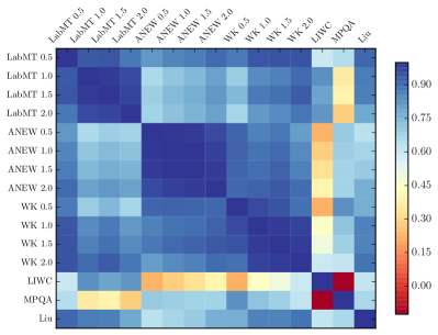
Figure 9: Pearson’s $r$ correlation between daily resolution Twitter sentiment time series for each dictionary. We see that there is strong agreement within dictionaries, with the biggest differences coming from the stop value of $\Delta h=0.5$. The LabMT and OL dictionaries do not strongly disagree with any of the others, while LIWC is the least correlated overall with other dictionaries. LabMT and OL correlate strongly with each other, and disagree most with the ANEW, LIWC, and MPQA dictionaries. The two least correlated dictionaries are the LIWC and MPQA dictionaries. Again, since there is no publicly accessible ground truth for Twitter sentiment, we compare dictionaries against the others, and look at the words. With these criteria, we find the LabMT dictionary to be the most useful.

All of the dictionaries are choppy at the start of the time frame, when Twitter volume is low in 2008 and into 2009. As more people join Twitter and the tweet volume increases through 2010, we see that LIWC rates the text as happier, while the rest start a slow decline in rating that is led by MPQA in the negative direction. In 2010, the LIWC dictionary is more positive than the rest with words like “haha”, “lol” and “hey” being used more frequently and swearing being less frequent than the all years of Twitter put together. The other dictionaries with more coverage find a decrease in positive words to balance this increase, with the exception of MPQA which finds many negative words going up in frequency (see 2010 word shift Figure in Appendix S7). All of the dictionaries agree most strongly in 2012, all finding a lot of negative language and swearing that brings scores down (see 2012 word shift Figure in Appendix S7). From the bottom at 2012, LIWC continues to go downward while the others trend back up. The signal from MPQA jumps to the most positive, and LIWC does start trending back up eventually. We analyze the words in 2014 with a word shift against all 7 years of tweets for each dictionary in each panel in the 2014 word shift Figure in Appendix S7: A. LabMT finds 2014 with less happy with more negative language. B. ANEW finds it happier with a few positive words up. C. WK finds it happier with more negative words (like LabMT). D. MPQA finds it more positive with less negative words. E. LIWC finds it less positive with more negative and less positive words. F. OL finds it to be of the same sentiment as the background with a balance in positive and negative word usage. From these word shifts, we can analyze which words cause MPQA and LIWC to disagree with the other dictionaries: the disagreement of MPQA is again marred by broad stem matches, and the disagreement of LIWC is due to a lack of coverage.

III.5 Brief Comparison to Machine Learning Methods

We implement a Naive Bayes (NB) classifier (sometimes harshly called idiot Bayes hand2001idiot ) on the tagged movie review dataset, using 10% of the reviews for training and then testing performance on the rest. Following standard practice, we remove the top 30 ranked words (“stop words”) from the 5000 most frequent words, and use the remaining 4970 words in our classifier for maximum performance (we observe a 0.5% improvement). Our implementation is analogous to those found in common Python natural language processing packages (see “NLTK” or “TextBlob” bird2006nltk ).

As we should expect, at the level of single review, NB outperforms the dictionary-based methods with a classification accuracy of 75.7% averaged over 100 trials. As the number of reviews is increased, the overlap from NB diminishes, and using our simple “fraction overlapping” metric, the error drops to 0 with more than 200 reviews. Interestingly, NB starts to do worse with more reviews put together, and with more than 500 of the 1000 reviews put together, it rates both the positive and negative reviews as positive (Figure in S8 Appendix).

The rating curves do not touch, and neither do the error bars, but they both go very slightly above 0. Overall, with Naive Bayes we are able to classify a higher percentage of individual reviews correctly, but with more variance.

In the two Tables in S8 Appendix we compute the words which the NB classifier uses to classify all of the positive reviews as positive, and all of the negative reviews as positive. The Natural Language Toolkit bird2006nltk implements a method to obtain the “most informative” words, by taking the ratio of the likelihood of words between all available classes, and looking for the largest ratio:

$$\max_{\textnormal{all words }w}\frac{P(w|c_{i})}{P(w|c_{j})}$$ (3)

for all combinations of classes $c_{i},c_{j}$. This is possible because of the “naive” assumption that feature (word) likelihoods are independent, resulting in a classification metric that is linear for each feature. In S8 Appendix, we provide the derivation of this linearity structure.

We find that the trained NB classifier relies heavily on words that are very specific to the training set including the names of actors of the movies themselves, making them useful as classifiers but not in understanding the nature of the text. We report the top 10 words for both positive and negative classes using both the ratio and difference methods in Table in S8 Appendix. To classify a document using NB, we use the frequency of each word in the document in conjunction with the probability that that word occurred in each labeled class $c_{i}$.

We next take the movie-review-trained NB classifier and use it to classify the New York Times sections, both by ranking them and by looking at the words (the above ratio and difference weighted by the occurrence of the words). We ranked the sections 5 different times, and among those find the “Television” section both by far the happiest, and by far the least happy in independent tests. We show these rankings and report the top 10 words used to score the “Society” section in Table S3.

We thus see that the NB classifier, a linear learning method, may perform poorly when assessing sentiment outside of the corpus on which it is trained. In general, performance will vary depending on the statistical dissimilarity of the training and novel corpora. Added to this is the inscrutability of black box methods: while susceptible to the aforementioned difficulty, nonlinear learning methods (unlike NB) also render detailed examination of how individual words contribute to a text’s score more difficult.

IV Conclusion

We have shown that measuring sentiment in various corpora presents unique challenges, and that dictionary performance is situation dependent. Across the board, the ANEW dictionary performs poorly, and the continued use of this dictionary with clearly better alternatives is a questionable choice. We have seen that the MPQA dictionary does not agree with the other five dictionaries on the NYT corpus and Twitter corpus due to a variety of context and stem matching issues, and we would not recommend using this dictionary. And in comparison to LabMT, the WK, LIWC, and OL dictionaries fail to provide much detail in corpora where their coverage is lower, including all four corpora tested. Sufficient coverage is essential or producing meaningful word shifts and thereby enabling deeper understanding.

In each case, to analyze the output of the dictionary method, we rely on the use of word shift graphs. With this tool, we can produce a finer grained analysis of the lexical content, and we can also detect words that are used out of context and can mask them directly. It should be clear that using any of the dictionary-based sentiment detecting method without looking at how individual words contribute is indefensible, and analyses that do not use word shifts or similar tools cannot be trusted. The poor word shift performance of binary dictionaries in particular gravely limits their ability to reveal underlying stories.

In sum, we believe that dictionary-based methods will continue to play a powerful role—they are fast and well suited for web-scale data sets—and that the best instruments will be based on dictionaries with excellent coverage and continuum scores. To this end, we urge that all dictionaries should be regularly updated to capture changing lexicons, word usage, and demographics. Looking further ahead, a move from scoring words to scoring both phrases and words should realize considerable improvement for many languages of interest. With phrase dictionaries, the resulting phrase shift graphs will allow for a more nuanced and detailed analysis of a corpus’s sentiment score alajajian2015a , ultimately affording clearer stories for sentiment dynamics.

S1 Appendix: Computational methods

All of the code to perform these tests is available and document on GitHub. The repository can be found here: https://github.com/andyreagan/sentiment-analysis-comparison.

Stem matching

Of the dictionaries tested, both LIWC and MPQA use “word stems”. Here we quickly note some of the technical difficulties with using word stems, and how we processed them, for future research to build upon and improve.

An example is abandon*, which is intended to the match words of the standard RE form abandon[a-z]*. A naive approach is to check each word against the regular expression, but this is prohibitively slow. We store each of the dictionaries in a “trie” data structure with a record. We use the easily available “marisa-trie” Python library, which wraps the C++ counterpart. The speed of these libraries made the comparison possible over large corpora, in particular for the dictionaries with stemmed words, where the prefix search is necessary. Specifically, the “trie” structure is 70 times faster than a regular expression based search for stem words. In particular, we construct two tries for each dictionary: a fixed and stemmed trie. We first attempt to match words against the fixed list, and then turn to the prefix match on the stemmed list.

Regular expression parsing

The first step in processing the text of each corpora is extracting the words from the raw text. Here we rely on a regular expression search, after first removing some punctuation. We choose to include a set of all characters that are found within the words in each of the six dictionaries tested in detail, such that it respects the parse used to create these dictionaries by retaining such characters. This takes the following form in Python, for raw_text as a string (note, pdflatex renders correctly locally, but arXiv seems to explode the link match group):

punctuation_to_replace = ["---","--","’’"]
for punctuation in punctuation_to_replace:
    raw_text = raw_text.replace(punctuation," ")
words = [x.lower() for x in re.findall(r"(?:[0-9][0-9,\.]*[0-9])|
                                         (?:http://[\w\./\-\?\&\#]+)|
                                         (?:[\w\@\#\’\&\]\[]+)|
                                         (?:[b}/3D;p)|’\-@x#^_0\\P(o:O{X$[=<>\]*B]+)",
                                       raw_text,flags=re.UNICODE)]

S2 Appendix: Continued individual comparisons

Picking up right where we left off in Section III, we next compare ANEW with the other dictionaries. The ANEW-WK comparison in Panel I of Fig. 1 contains all 1030 words of ANEW, with a fit of $h_{w_{\text{ANEW}}}=1.07*h_{w_{\text{WK}}}-0.30$, making ANEW more positive and with increasing positivity for more positive words. The 20 most different scores are (ANEW,WK): fame (7.93,5.45), god (8.15,5.90), aggressive (5.10,3.08), casino (6.81,4.68), rancid (4.34,2.38), bees (3.20,5.14), teacher (5.68,7.37), priest (6.42,4.50), aroused (7.97,5.95), skijump (7.06,5.11), noisy (5.02,3.21), heroin (4.36,2.74), insolent (4.35,2.74), rain (5.08,6.58), patient (5.29,6.71), pancakes (6.08,7.43), hospital (5.04,3.52), valentine (8.11,6.40), and book (5.72,7.05). We again see some of the same words from the LabMT comparisons with these dictionaries, and again can attribute some differences to small sample sizes and differing demographics.

For the ANEW-MPQA comparison in Panel J of Fig. 1 we show the same matched word lists as before. The happiest 10 words in ANEW matched by MPQA are: clouds (6.18), bar (6.42), mind (6.68), game (6.98), sapphire (7.00), silly (7.41), flirt (7.52), rollercoaster (8.02), comedy (8.37), laughter (8.45). The least happy 5 neutral words and happiest 5 neutral words in MPQA, matched with MPQA, are: pressure (3.38), needle (3.82), quiet (5.58), key (5.68), alert (6.20), surprised (7.47), memories (7.48), knowledge (7.58), nature (7.65), engaged (8.00), baby (8.22). The least happy words in ANEW with score +1 in MPQA that are matched by MPQA are: terrified (1.72), meek (3.87), plain (4.39), obey (4.52), contents (4.89), patient (5.29), reverent (5.35), basket (5.45), repentant (5.53), trumpet (5.75). Again we see some very questionable matches by the MPQA dictionary, with broad stems capturing words with both positive and negative scores.

For the ANEW-LIWC comparison in Panel K of Fig. 1 we show the same matched word lists as before. The happiest 10 words in ANEW matched by LIWC are: lazy (4.38), neurotic (4.45), startled (4.50), obsession (4.52), skeptical (4.52), shy (4.64), anxious (4.81), tease (4.84), serious (5.08), aggressive (5.10). There are only 5 words in ANEW that are matched by LIWC with LIWC score of 0: part (5.11), item (5.26), quick (6.64), couple (7.41), millionaire (8.03). The least happy words in ANEW with score +1 in LIWC that are matched by LIWC are: heroin (4.36), virtue (6.22), save (6.45), favor (6.46), innocent (6.51), nice (6.55), trust (6.68), radiant (6.73), glamour (6.76), charm (6.77).

For the ANEW-Liu comparison in Panel L of Fig. 1 we show the same matched word lists as before, except the neutral word list because Liu has no explicit neutral words. The happiest 10 words in ANEW matched by Liu are: pig (5.07), aggressive (5.10), tank (5.16), busybody (5.17), hard (5.22), mischief (5.57), silly (7.41), flirt (7.52), rollercoaster (8.02), joke (8.10). The least happy words in ANEW with score +1 in Liu that are matched by Liu are: defeated (2.34), obsession (4.52), patient (5.29), reverent (5.35), quiet (5.58), trumpet (5.75), modest (5.76), humble (5.86), salute (5.92), idol (6.12).

For the WK-MPQA comparison in Panel P of Fig. 1 we show the same matched word lists as before. The happiest 10 words in WK matched by MPQA are: cutie (7.43), pancakes (7.43), panda (7.55), laugh (7.56), marriage (7.56), lullaby (7.57), fudge (7.62), pancake (7.71), comedy (8.05), laughter (8.05). The least happy 5 neutral words and happiest 5 neutral words in MPQA, matched with MPQA, are: sociopath (2.44), infectious (2.63), sob (2.65), soulless (2.71), infertility (3.00), thinker (7.26), knowledge (7.28), legacy (7.38), surprise (7.44), song (7.59). The least happy words in WK with score +1 in MPQA that are matched by MPQA are: kidnapper (1.77), kidnapping (2.05), kidnap (2.19), discriminating (2.33), terrified (2.51), terrifying (2.63), terrify (2.84), courtroom (2.84), backfire (3.00), indebted (3.21).

For the WK-LIWC comparison in Panel Q of Fig. 1 we show the same matched word lists as before. The happiest 10 words in WK matched by LIWC are: geek (5.56), number (5.59), fiery (5.70), trivia (5.70), screwdriver (5.76), foolproof (5.82), serious (5.88), yearn (5.95), dumpling (6.48), weeping willow (6.53). The least happy 5 neutral words and happiest 5 neutral words in LIWC, matched with LIWC, are: negative (2.52), negativity (2.74), quicksand (3.62), lack (3.68), wont (4.09), unique (7.32), millionaire (7.32), first (7.33), million (7.55), rest (7.86). The least happy words in WK with score +1 in LIWC that are matched by LIWC are: heroin (2.74), friendless (3.15), promiscuous (3.32), supremacy (3.48), faithless (3.57), laughingstock (3.77), promiscuity (3.95), tenderfoot (4.26), succession (4.52), dynamite (4.79).

For the WK-Liu comparison in Panel R of Fig. 1 we show the same matched word lists as before, except the neutral word list because Liu has no explicit neutral words. The happiest 10 words in WK matched by Liu are: goofy (6.71), silly (6.72), flirt (6.73), rollercoaster (6.75), tenderness (6.89), shimmer (6.95), comical (6.95), fanciful (7.05), funny (7.59), fudge (7.62), joke (7.88). The least happy words in WK with score +1 in Liu that are matched by Liu are: defeated (2.59), envy (3.05), indebted (3.21), supremacy (3.48), defeat (3.74), overtake (3.95), trump (4.18), obsession (4.38), dominate (4.40), tough (4.45).

Now we’ll focus our attention on the MPQA row, and first we see comparisons against the three full range dictionaries. For the first match against LabMT in Panel D of Fig. 1, the MPQA match catches 431 words with MPQA score 0, while LabMT (without stems) matches 268 words in MPQA in Panel S (1039/809 and 886/766 for the positive and negative words of MPQA). Since we’ve already highlighted most of these words, we move on and focus our attention on comparing the $\pm 1$ dictionaries.

In Panels V–X, BB–DD, and HH–JJ of Fig. 1 there are a total of 6 bins off of the diagonal, and we focus out attention on the bins that represent words that have opposite scores in each of the dictionaries. For example, consider the matches made my MPQA in Panel BB: the words in the top left corner and bottom right corner with are scored in a opposite manner in LIWC, and are of particular concern. Looking at the words from Panel W with a +1 in MPQA and a -1 in LIWC (matched by LIWC) we see: stunned, fiery, terrified, terrifying, yearn, defense, doubtless, foolproof, risk-free, exhaustively, exhaustive, blameless, low-risk, low-cost, lower-priced, guiltless, vulnerable, yearningly, and yearning. The words with a -1 in MPQA that are +1 in LIWC (matched by LIWC) are: silly, madly, flirt, laugh, keen, superiority, supremacy, sillily, dearth, comedy, challenge, challenging, cheerless, faithless, laughable, laughably, laughingstock, laughter, laugh, grating, opportunistic, joker, challenge, flirty.

In Panel W of 1, the words with a +1 in MPQA and a -1 in Liu (matched by Liu) are: solicitude, flair, funny, resurgent, untouched, tenderness, giddy, vulnerable, and joke. The words with a -1 in MPQA that are +1 in Liu, matched by Liu, are: superiority, supremacy, sharp, defeat, dumbfounded, affectation, charisma, formidable, envy, empathy, trivially, obsessions, and obsession.

In Panel BB of 1, the words with a +1 in LIWC and a -1 in MQPA (matched by MPQA) are: silly, madly, flirt, laugh, keen, determined, determina, funn, fearless, painl, cute, cutie, and gratef. The words with a -1 in LIWC and a +1 in MQPA, that are matched by MPQA, are: stunned, terrified, terrifying, fiery, yearn, terrify, aversi, pressur, careless, helpless, and hopeless.

In Panel DD of 1, the words with a -1 in LIWC and a +1 in Liu, that are matched by Liu, are: silly, and madly. The words with a +1 in LIWC and a -1 in Liu, that are matched by Liu, are: stunned, and fiery.

In Panel HH of 1, the words with a -1 in Liu and a +1 in MPQA, that are matched by MPQA, are: superiority, supremacy, sharp, defeat, dumbfounded, charisma, affectation, formidable, envy, empathy, trivially, obsessions, obsession, stabilize, defeated, defeating, defeats, dominated, dominates, dominate, dumbfounding, cajole, cuteness, faultless, flashy, fine-looking, finer, finest, panoramic, pain-free, retractable, believeable, blockbuster, empathize, err-free, mind-blowing, marvelled, marveled, trouble-free, thumb-up, thumbs-up, long-lasting, and viewable. The words with a +1 in Liu and a -1 in MPQA, that are matched by MPQA, are: solicitude, flair, funny, resurgent, untouched, tenderness, giddy, vulnerable, joke, shimmer, spurn, craven, aweful, backwoods, backwood, back-woods, back-wood, back-logged, backaches, backache, backaching, backbite, tingled, glower, and gainsay.

In Panel II of 1, the words with a +1 in Liu and a -1 in LIWC, that are matched by LIWC, are: stunned, fiery, defeated, defeating, defeats, defeat, doubtless, dominated, dominates, dominate, dumbfounded, dumbfounding, faultless, foolproof, problem-free, problem-solver, risk-free, blameless, envy, trivially, trouble-free, tougher, toughest, tough, low-priced, low-price, low-risk, low-cost, lower-priced, geekier, geeky, guiltless, obsessions, and obsession. The words with a -1 in Liu and a +1 in LIWC, that are matched by LIWC, are: silly, madly, sillily, dearth, challenging, cheerless, faithless, flirty, flirt, funnily, funny, tenderness, laughable, laughably, laughingstock, grating, opportunistic, joker, and joke.

In the off-diagonal bins for all of the $\pm 1$ dictionaries, we see many of the same words. Again MPQA stem matches are disparagingly broad. We also find matches by LIWC that are concerning, and should in all likelihood be removed from the dictionary.

S3 Appendix: Coverage for all corpuses

We provide coverage plots for the other three corpuses.

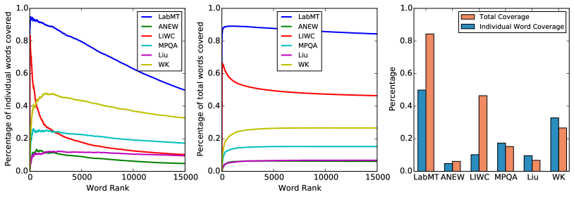
Figure S1: Coverage of the words on twitter by each of the dictionaries.

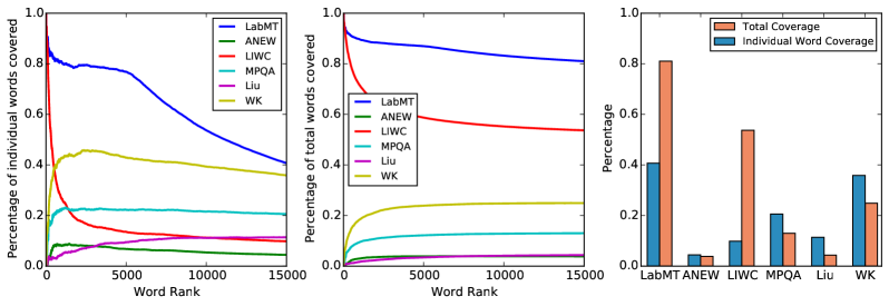
Figure S2: Coverage of the words in Google books by each of the dictionaries.

S4 Appendix: Sorted New York Times rankings

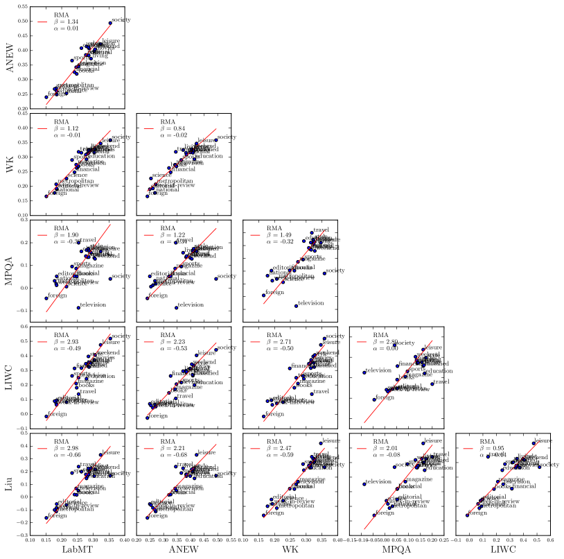
Figure S4: NYT Sections scatterplot. The RMA fit $\alpha$ and $\beta$ for the formula $y=\alpha+\beta x$. For the sake of comparison, we normalized each dictionary to the range [-.5,.5] by subtracting the mean score (5 or 0) and dividing by the range (8 or 2).

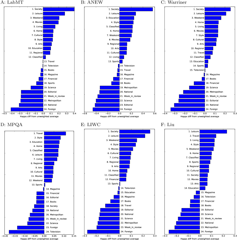
Figure S5: Sorted bar charts ranking each of the 24 New York Times Sections for each dictionary tested.

S5 Appendix: Movie Review Distributions

Here we examine the distributions of movie review scores. These distributions are each summarized by their mean and standard deviation in panels of Figure 2 for each dictionary. For example, the left most error bar of each panel in Figure 2 shows the standard deviation around the mean for the distribution of individual review scores (Figure S6).

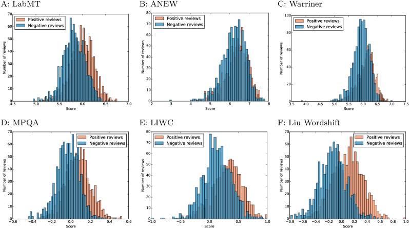
Figure S6: Binned scores for each review by each corpus with a stop value of $\Delta_{h}=1.0$.

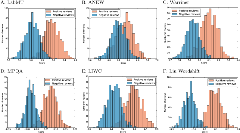
Figure S7: Binned scores for samples of 15 concatenated random reviews. Each dictionary uses stop value of $\Delta_{h}=1.0$.

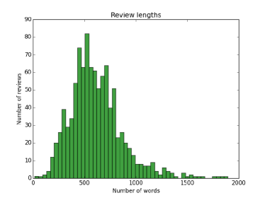
Figure S8: Binned length of positive reviews, in words.

S6 Appendix: Google Books correlations and word shifts

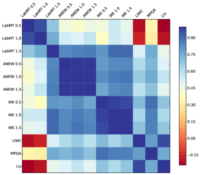
Figure S9: Google Books correlations. Here we include correlations for the google books time series, and word shifts for selected decades (1920’s,1940’s,1990’s,2000’s).

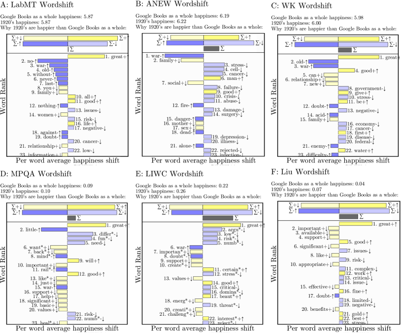
Figure S10: Google Books shifts in the 1920’s against the baseline of Google Books.

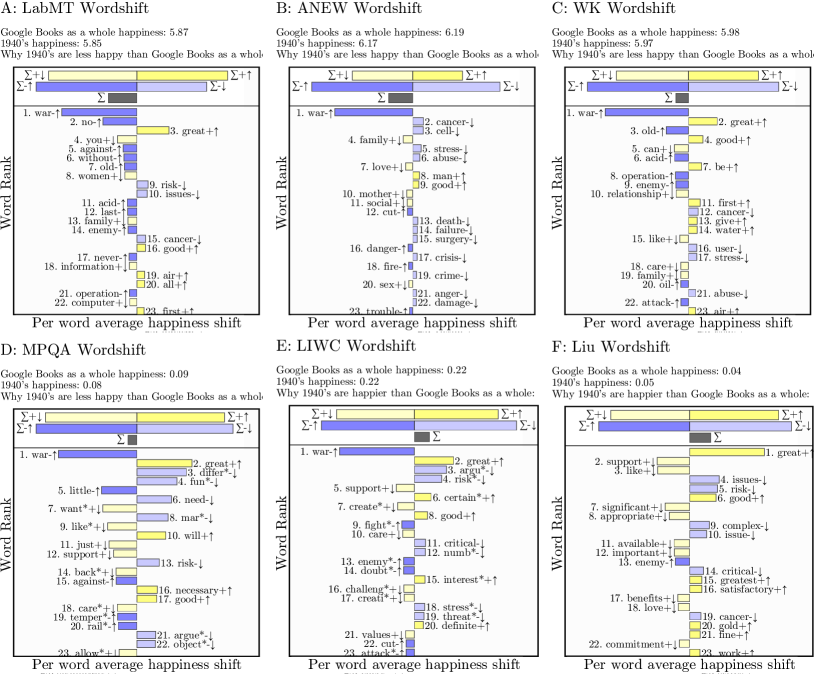
Figure S11: Google Books shifts in the 1940’s against the baseline of Google Books.

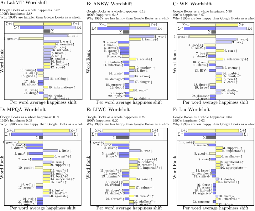
Figure S12: Google Books shifts in the 1990’s against the baseline of Google Books.

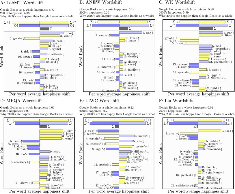
Figure S13: Google Books shifts in the 2000’s against the baseline of Google Books.

S7 Appendix: Additional Twitter time series, correlations, and shifts

First, we present additional Twitter time series:

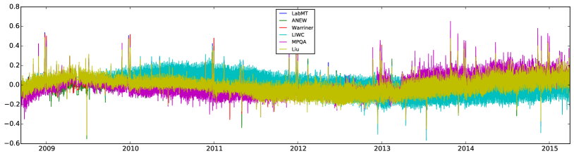
Figure S14: Normalized time series on Twitter using $\Delta_{h}$ of 1.0 for all. For resolution of 3 hours. We do not include any of the time series with resolution below 3 hours here because there are too many data points to see.

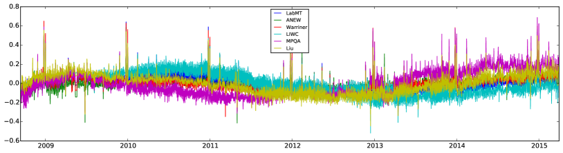
Figure S15: Normalized time series on Twitter using $\Delta_{h}$ of 1.0 for all. For resolution of 12 hours.

Next, we take a look at more correlations:

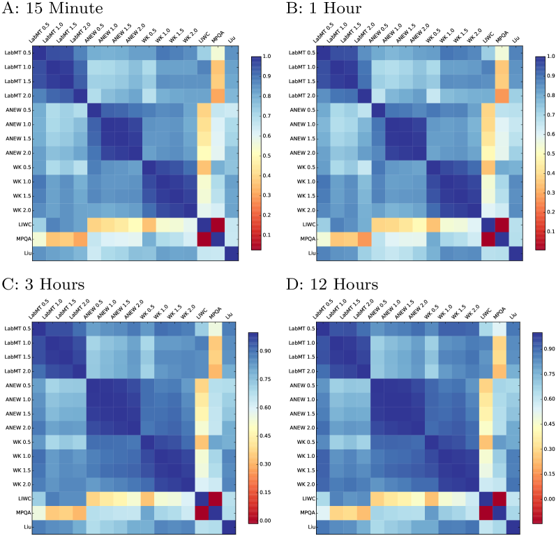
Figure S16: Pearson’s $r$ correlation between Twitter time series for all resolutions below 1 day.

Now we include word shift graphs that are absent from the manuscript itself.

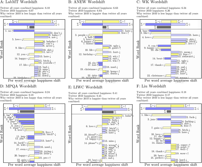
Figure S17: Word Shifts for Twitter in 2010. The reference word usage is all of Twitter (the 10% Gardenhose feed) from September 2008 through April 2015, with the word usage normalized by year.

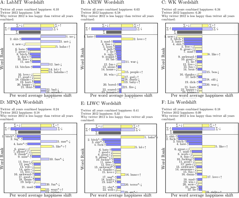
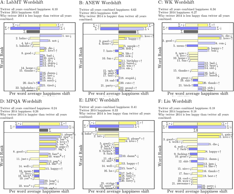
Figure S18: Word Shifts for Twitter in 2012. The reference word usage is all of Twitter (the 10% Gardenhose feed) from September 2008 through April 2015, with the word usage normalized by year.

Figure S19: Word Shifts for Twitter in 2014. The reference word usage is all of Twitter (the 10% Gardenhose feed) from September 2008 through April 2015, with the word usage normalized by year.

Finally, we include the results of each dictionary applied to a set of annotated Twitter data. We apply sentiment dictionaries to rate individual tweets and classify a tweet as positive (negative) if the tweet rating is greater (less) than the average of all scores in dictionary.

Rank	Dictionary	% tweets scored	F1 of tweets scored	Calibrated F1	Overall F1
1.	Sent140Lex	100.0	0.89	0.88	0.89
2.	labMT	100.0	0.69	0.78	0.69
3.	HashtagSent	100.0	0.67	0.64	0.67
4.	SentiWordNet	98.6	0.67	0.68	0.67
5.	VADER	81.3	0.75	0.81	0.61
6.	SentiStrength	73.9	0.83	0.81	0.61
7.	SenticNet	97.3	0.61	0.64	0.59
8.	Umigon	67.1	0.87	0.85	0.58
9.	SOCAL	82.2	0.71	0.75	0.58
10.	WDAL	99.9	0.58	0.64	0.58
11.	AFINN	73.6	0.78	0.80	0.57
12.	OL	66.7	0.83	0.82	0.55
13.	MaxDiff	94.1	0.58	0.70	0.54
14.	EmoSenticNet	96.0	0.56	0.59	0.54
15.	MPQA	73.2	0.73	0.72	0.53
16.	WK	96.5	0.53	0.72	0.51
17.	LIWC15	61.8	0.81	0.78	0.50
18.	Pattern	69.0	0.71	0.75	0.49
19.	GI	67.6	0.72	0.70	0.49
20.	LIWC07	60.3	0.80	0.75	0.48
21.	LIWC01	54.3	0.83	0.75	0.45
22.	EmoLex	59.4	0.73	0.69	0.43
23.	ANEW	64.1	0.65	0.68	0.42
24.	USent	4.5	0.74	0.73	0.03
25.	PANAS-X	1.7	0.88	–	0.01
26.	Emoticons	1.4	0.72	0.77	0.01

Table S1: Ranked results of sentiment dictionary performance on individual tweets from STS-Gold dataset (Saif, 2013). We report the percentage of tweets for which each dictionary contains at least 1 entry, the F1 score on those tweets, and the overall classification F1 score. The calibrated F1 score tunes the decision threshold between positive and negative tweets with a random 10% training sample.

S8 Appendix: Naive Bayes results and derivation

We now provide more details on the implementation of Naive Bayes, a derivation of the linearity structure, and more results from the classification of Movie Reviews.

First, to implement a binary Naive Bayes classifier for a collection of documents, we denote each of the $N$ words in the given document $T$ as $w_{i}$, the word frequency as $f_{i}(T)$, and class labels $c_{1},c_{2}$. The probability of a document $T$ belonging to class $c_{1}$ can be written as

$$P(c_{1}|T)=\frac{P(c_{1})P(T|c_{1})}{P(T)}.$$

Since we do not know $P(T|c_{1})$ explicitly, we make the naive assumption that each word appears independently, and thus write

$$P(c_{1}|T)=\frac{P(c_{1})\cdot\left[P(f_{1}(T)|c_{1})\cdot P(f_{2}(T)|c_{1})\cdots P(f_{N}(T)|c_{1})\right]}{P(T)}.$$

Since we are only interested in comparing $P(c_{1}|T)$ and $P(c_{2}|T)$, we disregard the shared denominator and have

$$P(c_{1}|T)\propto P(c_{1})\cdot\left[P(f_{1}(T)|c_{1})\cdot P(f_{2}(T)|c_{1})\cdots P(f_{N}(T)|c_{1})\right].$$

Finally we say that document $T$ belongs to class $c_{1}$ if $P(c_{1}|T)>P(c_{2}|T)$. Given that the probabilities of individual words are small, to avoid machine truncation error we compute these probabilities in log space, such that the product of individual word likelihoods becomes a sum

$$\log P(c_{1}|T)\propto\log P(c_{1})+\sum_{i=1}^{N}P(f_{i}(T)|c_{1}).$$

Assigning a classification of class $c_{1}$ if $P(c_{1}|T)>P(c_{2}|T)$ is the same as saying that the difference between the two is positive, i.e. $P(c_{1}|T)-P(c_{2}|T)>0$ and since the logarithm is monotonic, $\log P(c_{1}|T)-\log P(c_{2}|T)>0$. To examine how individual words contribute to this difference, we can write

$$0 <\log P(c_{1}|T)-\log P(c_{2}|T)$$

$$\propto\log P(c_{1})+\sum_{i=1}^{N}\log P(f_{i}(T)|c_{1})-\log P(c_{2})-\sum_{i=1}^{N}\log P(f_{i}(T)|c_{2})$$

$$\propto\log P(c_{1})-\log P(c_{2})+\sum_{i=1}^{N}\left[\log P(f_{i}(T)|c_{1})\log P(f_{i}(T)|c_{2})\right]$$

$$\propto\log\frac{P(c_{1})}{P(c_{2})}+\sum_{i=1}^{N}\log\frac{P(f_{i}(T)|c_{1})}{P(f_{i}(T)|c_{2})}.$$

We can see from the above that the contribution of each word $w_{i}$ (or more accurately, the likelihood of frequency in document $T$ being of class $c$ as $P(f_{i}(T)|c_{1})$) is a linear constituent of the classification.

Next, we include the detailed results of the Naive Bayes classifier on the Movie Review corpus.

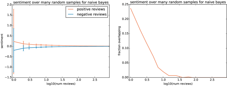
Figure S20: Results of the NB classifier on the Movie Reviews corpus.

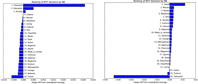
Figure S21: NYT Sections ranked by Naive Bayes in two of the five trials.

Most informative
Positive		Negative
Word	Value	Word	Value
27.27	flynt	20.21	godzilla
26.33	truman	15.95	werewolf
20.68	charles	13.83	gorilla
15.04	event	13.83	spice
14.10	shrek	13.83	memphis
13.16	cusack	13.83	sgt
13.16	bulworth	12.76	jennifer
13.16	robocop	12.76	hill
12.22	jedi	11.70	max
12.22	gangster	11.70	200

NYT Society
Positive		Negative
Word	Value	Word	Value
26.08	truman	20.40	godzilla
20.49	charles	12.88	hill
12.11	gangster	12.88	jennifer
10.25	speech	10.73	fatal
9.32	melvin	8.59	freddie
8.85	wars	8.59	=
7.45	agents	8.59	mess
6.52	dance	8.59	gene
6.52	bleak	8.59	apparent
6.52	pitt	7.51	travolta

Table S2: Trial 1 of Naive Bayes trained on a random 10% of the movie review corpus, and applied to the New York Times Society section. We show the words which are used by the trained classifier to classify individual reviews (in corpus), and on the New York Times (out of corpus). In addition, we report a second trial in Table S3, since Naive Bayes is trained on a random subset of data, to show the variation in individual words between trials (while performance is consistent).

Most informative
Positive		Negative
Word	Value	Word	Value
18.11	shrek	34.63	west
17.15	poker	24.14	webb
15.25	shark	18.89	jackal
14.29	maggie	17.84	travolta
13.34	guido	17.84	woo
13.34	outstanding	17.84	coach
13.34	political	16.79	awful
13.34	journey	16.79	brenner
13.34	bulworth	15.74	gabriel
12.39	bacon	15.74	general’s

NYT Society
Positive		Negative
Word	Value	Word	Value
17.79	poker	33.39	west
13.84	journey	17.20	coach
13.84	political	17.20	travolta
8.90	tribe	15.18	gabriel
7.91	tony	12.14	pointless
7.91	price	9.44	stupid
7.91	threat	8.09	screaming
7.12	titanic	7.59	mess
6.92	dicaprio	7.42	boring
6.92	kate	7.08	=

Table S3: Trial 2 of Naive Bayes trained on a random 10% of the movie review corpus, and applied to the New York Times Society section. We show the words which are used by the trained classifier to classify individual reviews (in corpus), and on the New York Times (out of corpus). This second trial is in addition to the first trial in Table S2, since Naive Bayes is trained on a random subset of data, to show the variation in individual words between trials (while performance is consistent).

S9 Appendix: Movie review benchmark of additional dictionaries

Here, we present the accuracy of each dictionary applied to binary classification of Movie Reviews.

Rank	Title	% Scored	F1 Trained	F1 Untrained
1.	OL	100	0.70	0.71
2.	HashtagSent	100	0.67	0.66
3.	MPQA	100	0.67	0.66
4.	SentiWordNet	100	0.65	0.65
5.	labMT	100	0.64	0.63
6.	AFINN	100	0.67	0.63
7.	Umigon	100	0.65	0.62
8.	GI	100	0.65	0.61
9.	SOCAL	100	0.71	0.60
10.	VADER	100	0.67	0.60
11.	WDAL	100	0.60	0.59
12.	SentiStrength	100	0.63	0.58
13.	EmoLex	100	0.65	0.56
14.	LIWC15	100	0.64	0.55
15.	LIWC01	100	0.65	0.54
16.	LIWC07	100	0.64	0.53
17.	Pattern	100	0.73	0.52
18.	PANAS-X	33	0.51	0.51
19.	Sent140Lex	100	0.68	0.47
20.	SenticNet	100	0.62	0.45
21.	ANEW	100	0.57	0.36
22.	MaxDiff	100	0.66	0.36
23.	EmoSenticNet	100	0.58	0.34
24.	WK	100	0.63	0.34
25.	Emoticons	0	–	–
26.	USent	40	–	–

Table S4: Ranked performance of dictionaries on the Movie Review corpus.

Rank	Title	% Scored	F1 Trained of Scored	F1 Untrained of Scored	F1 Untrained, All
1.	HashtagSent	100	0.55	0.55	0.55
2.	LIWC15	99	0.53	0.55	0.55
3.	LIWC07	99	0.53	0.55	0.54
4.	LIWC01	99	0.52	0.55	0.54
5.	labMT	99	0.54	0.54	0.54
6.	Sent140Lex	100	0.55	0.54	0.54
7.	SentiWordNet	99	0.54	0.53	0.53
8.	WDAL	99	0.53	0.53	0.52
9.	EmoLex	95	0.54	0.55	0.52
10.	MPQA	93	0.54	0.55	0.52
11.	SenticNet	97	0.53	0.52	0.50
12.	SOCAL	88	0.56	0.55	0.49
13.	EmoSenticNet	98	0.52	0.46	0.45
14.	Pattern	81	0.55	0.55	0.45
15.	GI	80	0.55	0.55	0.44
16.	WK	97	0.54	0.45	0.44
17.	OL	76	0.56	0.57	0.44
18.	VADER	79	0.56	0.55	0.43
19.	SentiStrength	77	0.54	0.54	0.41
20.	MaxDiff	83	0.54	0.49	0.41
21.	AFINN	70	0.56	0.56	0.39
22.	ANEW	63	0.52	0.48	0.30
23.	Umigon	53	0.56	0.56	0.30
24.	PANAS-X	1	0.53	0.53	0.01
25.	Emoticons	0	–	–	–
26.	USent	2	–	–	–

Table S5: Ranked performance of dictionaries on the Movie Review corpus, broken into sentences.

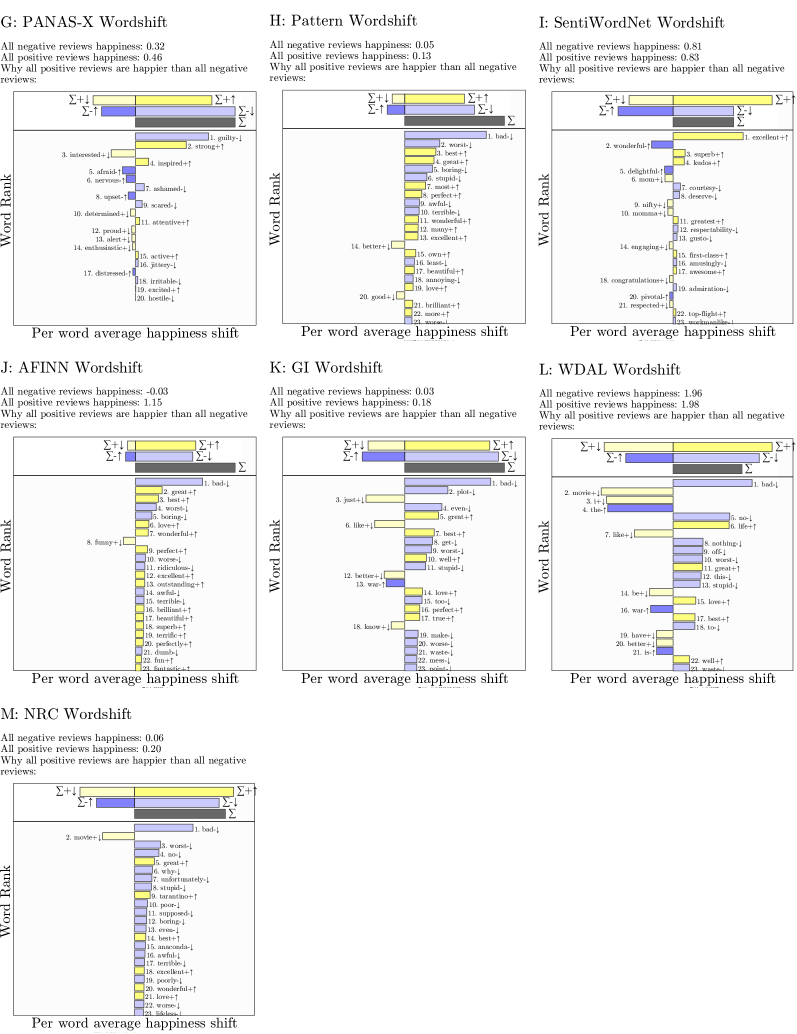
Figure S22: Word shifts for the movie review corpus, with panel letters continuing from Fig. 6. We again see many of the same patterns, and refer the reader to Fig. 6 for a more in depth analysis.

S10 Appendix: Coverage removal and binarization tests of labMT dictionary

Here, we perform a detailed analysis of the labMT dictionary to further isolate the effects of dictionary coverage and scoring type. This analysis is motivated by ensuring that the our results are not confounded entirely by the quality of the word scores across dictionaries, such that the effect of coverage and scoring type are isolated. We focus on the Movie Review corpus for this analysis, and report the accuracy of the labMT dictionary with the aforementioned modifications using the F1 score.

First, we gradually reduce the range of scores in the labMT dictionary from a centered -4 $\to$ 4, down to just the integer scores $-1$ and $1$. In Figure S23, the F1 score is show across this gradual, linear change to a binary dictionary. We observe that the direct binarization of the labMT dictionary results in a degradation of performance. Second, to test the effect of coverage alone, we systematically reduce the coverage of the labMT dictionary and again attempt the binary classification task of identifying Movie Review polarity. Three possible strategies to reduce the coverage are (1) removing the most frequent words, (2) removing the least frequent words, and (3) removing words randomly (irrespective of their frequency of usage). In Figures S24 and S25, we show the resulting F1 score of classification performance for each of these three strategies and the total coverage from each removal strategy. We observe that while certain strategies are more effective at retaining performance, lower coverage scores are all lower despite substantial variation, and the overall pattern for each strategy is a decrease in performance for decreasing coverage. In both cases these results are consistent with those seen across dictionaries: integer scores and low coverage strongly reduce the performance of the 2-class movie review classification task, as measured by the F1-score.

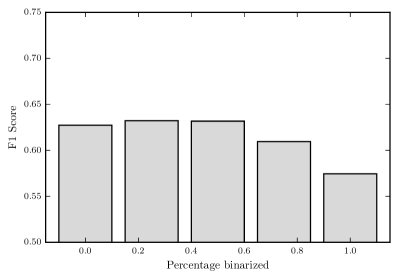
Figure S23: The direct binarization of the labMT dictionary results in a degradation of performance. The binarization is accomplished by linearly reducing the range of scores in the labMT dictionary from a centered -4 $\to$ 4 to the integer scores $-1$ and $1$.

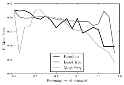
Figure S24: The resulting F1 score of classification performance for each of three coverage removal strategies. These strategies, labeled in the above, are: (1) removing the most frequent words, (2) removing the least frequent words, and (3) removing words randomly (irrespective of their frequency of usage).

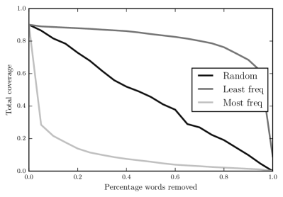
Figure S25: The resulting coverage for each of three coverage removal strategies. Again, these strategies, labeled in the above, are: (1) removing the most frequent words, (2) removing the least frequent words, and (3) removing words randomly (irrespective of their frequency of usage).

References

- (1) J. Bollen, H. Mao, and X. Zeng. Twitter mood predicts the stock market. Journal of Computational Science, 2(1):1–8, 2011.
- (2) J. Si, A. Mukherjee, B. Liu, Q. Li, H. Li, and X. Deng. Exploiting topic based Twitter sentiment for stock prediction. In ACL (2), pages 24–29, 2013.
- (3) S. Chung and S. Liu. Predicting stock market fluctuations from Twitter. Berkeley, California, 2011.
- (4) E. J. Ruiz, V. Hristidis, C. Castillo, A. Gionis, and A. Jaimes. Correlating financial time series with micro-blogging activity. In Proceedings of the fifth ACM international conference on Web search and data mining, pages 513–522. ACM, 2012.
- (5) P. S. Dodds, E. M. Clark, S. Desu, M. R. Frank, A. J. Reagan, J. R. Williams, L. Mitchell, K. D. Harris, I. M. Kloumann, J. P. Bagrow, K. Megerdoomian, M. T. McMahon, B. F. Tivnan, and C. M. Danforth. Human language reveals a universal positivity bias. PNAS, 112(8):2389–2394, 2015.
- (6) S. E. Alajajian, J. R. Williams, A. J. Reagan, S. C. Alajajian, M. R. Frank, L. Mitchell, J. Lahne, C. M. Danforth, and P. S. Dodds. The Lexicocalorimeter: Gauging public health through caloric input and output on social media. Available at http://arxiv.org/abs/1507.05098, 2016.
- (7) M. M. Bradley and P. J. Lang. Affective norms for english words (ANEW): Stimuli, instruction manual and affective ratings. Technical report c-1, University of Florida, Gainesville, FL, 1999.
- (8) J. W. Pennebaker, M. E. Francis, and R. J. Booth. Linguistic inquiry and word count: LIWC 2001. Mahway: Lawrence Erlbaum Associates, 71:2001, 2001.
- (9) T. Wilson, J. Wiebe, and P. Hoffmann. Recognizing contextual polarity in phrase-level sentiment analysis. Proceedings of Human Language Technologies Conference/Conference on Empirical Methods in Natural Language Processing (HLT/EMNLP 2005), 2005.
- (10) B. Liu. Sentiment analysis and subjectivity. Handbook of natural language processing, 2:627–666, 2010.
- (11) A. B. Warriner and V. Kuperman. Affective biases in English are bi-dimensional. Cognition and Emotion, pages 1–21, 2014.
- (12) R. Socher, A. Perelygin, J. Y. Wu, J. Chuang, C. D. Manning, A. Y. Ng, and C. Potts. Recursive deep models for semantic compositionality over a sentiment treebank. In Proceedings of the conference on empirical methods in natural language processing (EMNLP), volume 1631, page 1642. Citeseer, 2013.
- (13) P. S. Dodds and C. M. Danforth. Measuring the happiness of large-scale written expression: Songs, blogs, and presidents. Journal of Happiness Studies, 11(4):441–456, July 2009.
- (14) P. S. Dodds, K. D. Harris, I. M. Kloumann, C. A. Bliss, and C. M. Danforth. Temporal patterns of happiness and information in a global social network: Hedonometrics and Twitter. PLoS ONE, 6(12):e26752, 12 2011.
- (15) S. A. Golder and M. W. Macy. Diurnal and seasonal mood vary with work, sleep, and daylength across diverse cultures. Science Magazine, 333:1878–1881, 2011.
- (16) D. Garcia, A. Garas, and F. Schweitzer. The language-dependent relationship between word happiness and frequency. Proceedings of the National Academy of Sciences, 112(23):E2983, 2015.
- (17) P. S. Dodds, E. M. Clark, S. Desu, M. R. Frank, A. J. Reagan, J. R. Williams, L. Mitchell, K. D. Harris, I. M. Kloumann, J. P. Bagrow, K. Megerdoomian, M. T. McMahon, B. F. Tivnan, and C. M. Danforth. Reply to garcia et al.: Common mistakes in measuring frequency-dependent word characteristics. Proceedings of the National Academy of Sciences, 112(23):E2984–E2985, 2015.
- (18) S. P. Wojcik, A. Hovasapian, J. Graham, M. Motyl, and P. H. Ditto. Conservatives report, but liberals display, greater happiness. Science, 347(6227):1243–1246, 2015.
- (19) F. N. Ribeiro, M. Araújo, P. Gonçalves, M. A. Gonçalves, and F. Benevenuto. SentiBench - a benchmark comparison of state-of-the-practice sentiment analysis methods. EPJ Data Sci., 5(1), jul 2016.
- (20) B. Liu. Sentiment analysis and opinion mining. Synthesis lectures on human language technologies, 5(1):1–167, 2012.
- (21) D. Watson and L. A. Clark. The PANAS-X: Manual for the positive and negative affect schedule-expanded form: Manual for the positive and negative affect schedule-expanded form. PhD thesis, University of Iowa, 1999.
- (22) T. De Smedt and W. Daelemans. Pattern for Python. The Journal of Machine Learning Research, 13(1):2063–2067, 2012.
- (23) S. Baccianella, A. Esuli, and F. Sebastiani. SentiWordNet 3.0: An enhanced lexical resource for sentiment analysis and opinion mining. In LREC, volume 10, pages 2200–2204, 2010.
- (24) F. Å. Nielsen. A new ANEW: Evaluation of a word list for sentiment analysis in microblogs. In M. Rowe, M. Stankovic, A.-S. Dadzie, and M. Hardey, editors, CEUR Workshop Proceedings, volume Proceedings of the ESWC2011 Workshop on ’Making Sense of Microposts’: Big things come in small packages 718, pages 93–98, May 2011.
- (25) P. J. Stone, D. C. Dunphy, and M. S. Smith. The general inquirer: A computer approach to content analysis. MIT Press, 1966.
- (26) C. Whissell, M. Fournier, R. Pelland, D. Weir, and K. Makarec. A dictionary of affect in language: Iv. reliability, validity, and applications. Perceptual and Motor Skills, 62(3):875–888, 1986.
- (27) S. M. Mohammad and P. D. Turney. Crowdsourcing a word–emotion association lexicon. Computational Intelligence, 29(3):436–465, 2013.
- (28) S. Kiritchenko, X. Zhu, and S. M. Mohammad. Sentiment analysis of short informal texts. Journal of Artificial Intelligence Research, 50:723–762, 2014.
- (29) X. Zhu, S. Kiritchenko, and S. M. Mohammad. Nrc-canada-2014: Recent improvements in the sentiment analysis of tweets. In Proceedings of the 8th international workshop on semantic evaluation (SemEval 2014), pages 443–447. Citeseer, 2014.
- (30) S. M. Mohammad, S. Kiritchenko, and X. Zhu. Nrc-canada: Building the state-of-the-art in sentiment analysis of tweets. In Proceedings of the seventh international workshop on Semantic Evaluation Exercises (SemEval-2013), Atlanta, Georgia, USA, June 2013.
- (31) M. Taboada, J. Brooke, M. Tofiloski, K. Voll, and M. Stede. Lexicon-based methods for sentiment analysis. Computational linguistics, 37(2):267–307, 2011.
- (32) E. Cambria, D. Olsher, and D. Rajagopal. Senticnet 3: a common and common-sense knowledge base for cognition-driven sentiment analysis. In Proceedings of the twenty-eighth AAAI conference on artificial intelligence, pages 1515–1521. AAAI Press, 2014.
- (33) P. Gonçalves, M. Araújo, F. Benevenuto, and M. Cha. Comparing and combining sentiment analysis methods. In Proceedings of the first ACM conference on Online social networks, pages 27–38. ACM, 2013.
- (34) M. Thelwall, K. Buckley, G. Paltoglou, D. Cai, and A. Kappas. Sentiment strength detection in short informal text. Journal of the American Society for Information Science and Technology, 61(12):2544–2558, 2010.
- (35) C. J. Hutto and E. Gilbert. Vader: A parsimonious rule-based model for sentiment analysis of social media text. In Eighth International AAAI Conference on Weblogs and Social Media, 2014.
- (36) C. Levallois. Umigon: sentiment analysis for tweets based on terms lists and heuristics. In Second Joint Conference on Lexical and Computational Semantics (* SEM), volume 2, pages 414–417, 2013.
- (37) N. Pappas, G. Katsimpras, and E. Stamatatos. Distinguishing the popularity between topics: A system for up-to-date opinion retrieval and mining in the web. In International Conference on Intelligent Text Processing and Computational Linguistics, pages 197–209. Springer, 2013.
- (38) S. Poria, A. Gelbukh, A. Hussain, N. Howard, D. Das, and S. Bandyopadhyay. Enhanced senticnet with affective labels for concept-based opinion mining. IEEE Intelligent Systems, 28(2):31–38, 2013.
- (39) E. Sandhaus. The New York Times Annotated Corpus. Linguistic Data Consortium, Philadelphia, 2008.
- (40) B. Pang and L. Lee. A sentimental education: Sentiment analysis using subjectivity summarization based on minimum cuts. In Proceedings of the ACL, 2004.
- (41) Y. Lin, J.-B. Michel, E. L. Aiden, J. Orwant, W. Brockman, and S. Petrov. Syntactic annotations for the google books ngram corpus. In Proceedings of the ACL 2012 system demonstrations, pages 169–174. Association for Computational Linguistics, 2012.
- (42) L. Mitchell, M. R. Frank, K. D. Harris, P. S. Dodds, and C. M. Danforth. The Geography of Happiness: Connecting Twitter Sentiment and Expression, Demographics, and Objective Characteristics of Place. PLoS ONE, 8(5):e64417, May 2013.
- (43) J. M. V. Rayner. Linear relations in biomechanics: the statistics of scaling functions. J. Zool. Lond. (A), 206:415–439, 1985.
- (44) J.-B. Michel, Y. K. Shen, A. P. Aiden, A. Veres, M. K. Gray, J. P. Pickett, D. Hoiberg, D. Clancy, P. Norvig, J. Orwant, et al. Quantitative analysis of culture using millions of digitized books. Science, 331(6014):176–182, 2011.
- (45) E. A. Pechenick, C. M. Danforth, and P. S. Dodds. Characterizing the google books corpus: Strong limits to inferences of socio-cultural and linguistic evolution. arXiv preprint arXiv:1501.00960, 2015.
- (46) D. J. Hand and K. Yu. Idiot’s bayes—not so stupid after all? International statistical review, 69(3):385–398, 2001.
- (47) S. Bird. Nltk: the natural language toolkit. In Proceedings of the COLING/ACL on Interactive presentation sessions, pages 69–72. Association for Computational Linguistics, 2006.