Efficient Transition Adjacency Relation Computation for Process Model Similarity

Jisheng Pei, Lijie Wen, Xiaojun Ye, and Akhil Kumar L. Wen is the corresponding author with School of Software, Tsinghua University, Beijing 100084, China.
E-mail: wenlj@tsinghua.edu.cn J. Pei, X. Ye are with Tsinghua University and A. Kumar is with Penn State University.
Abstract

Many activities in business process management, such as process retrieval, process mining and process integration, need to determine the similarity between business processes. Along with many other relational behavior semantics, Transition Adjacency Relation (abbr. TAR) has been proposed as a kind of behavioral gene of process models and a useful perspective for process similarity measurement. In this article we explain why it is still relevant and necessary to improve TAR or pTAR (i.e., projected TAR) computation efficiency and put forward a novel approach for TAR computation based on Petri net unfolding. This approach not only improves the efficiency of TAR computation, but also enables the long-expected combined usage of TAR and Behavior Profiles (abbr. BP) in process model similarity estimation.

Index Terms:
Transition Adjacency Relation, Petri Net, Unfolding, Process Model Similarity.

1 Introduction

Since its first introduction [1], Transition Adjacency Relation (TAR) has been applied in a wide range of business process model analysis scenarios such as similarity measurement [2, 3, 4, 5, 6], process model retrieval [7, 8], and process mining [9, 10]. Different from conformance checking between a process model and an event log [11], a process similarity algorithm based on TAR (TAR similarity in short) takes two process models as the input and computes a similarity value ranging from 0.0 to 1.0 between them. Furthermore, TAR similarity is also different from workflow inheritance techniques [12], which also takes two process models as the input but tries to determine whether one process model is inherited from another. TAR in a Petri net simply defines the set of ordered pairs t1,t2subscript𝑡1subscript𝑡2\langle t_{1},t_{2}\rangle that can be executed one after another, but despite of its simplicity, the set of TARs reveal a useful perspective of the behaviors of the business process model. Later on, TAR was extended to projected Transition Adjacency Relation (pTAR) [2], which neglects the silent transitions so that users may selectively focus on a set of business-relevant transitions, and neglect the rest by marking them as silent transitions. However, both the original TAR computation algorithm [1] and pTAR computation algorithm [2] rely on exploiting the state-space of the process model by constructing its reachability graph (RG), which leaves the state-explosion caused by concurrencies as an unsolved problem.

On the other hand, Behavior Profiles (BP) [3] have been accepted in recent years as a most widely used relational semantics for business process analysis. It provides great descriptive power for process behaviors and can be efficiently computed with unfolding [4]). However, despite its various applications in scenarios such as consistency checking and similarity measurement, researchers have noticed the limitations to its expressive powers [9]. It has been discussed in several works that while some process models may have identical behavior profiles but produce different output traces.

As a result, a comprehensive relational semantics called 4C Spectrum has been proposed in [13] to make up for the missing expressive power of BP. Nevertheless, although 4C Spectrum is strong in terms of expressive power, it is a heavy-weight solution and contains hundreds of complex relations (resulted from the combination of co-occurrence and causal/concurrent patterns), which is costly to compute and difficult for users to grasp the insight intuitively. As a result, [13] has addressed the computation of only two of these relations, leaving most of the 4C Spectrum relations unavailable for application at this stage.

The above developments of relational semantics motivate us to look for a light-weight solution to significantly improve current relational semantics. In [6], it has been suggested that similarity estimation might benefit a lot from the combined usage of BP and TAR. Also, it is worthy of notice that there are only 4 types of relations in total even if consider BP together with TAR. However, this idea has not been broadly applied yet because TAR computation based on reachability graphs is extremely low in efficiency, and users may not want to sacrifice the high efficiency of BP even though considering TAR additionally may result in improvement of similarity estimation quality. To illustrate this, we will first demonstrate the advantage of TAR over BP. Motivated by this, we will go deeper into the issue of how to improve TAR computation efficiency.
Refer to caption
(a)
Refer to caption
(b)
Refer to caption
(c)
Refer to caption
(d)
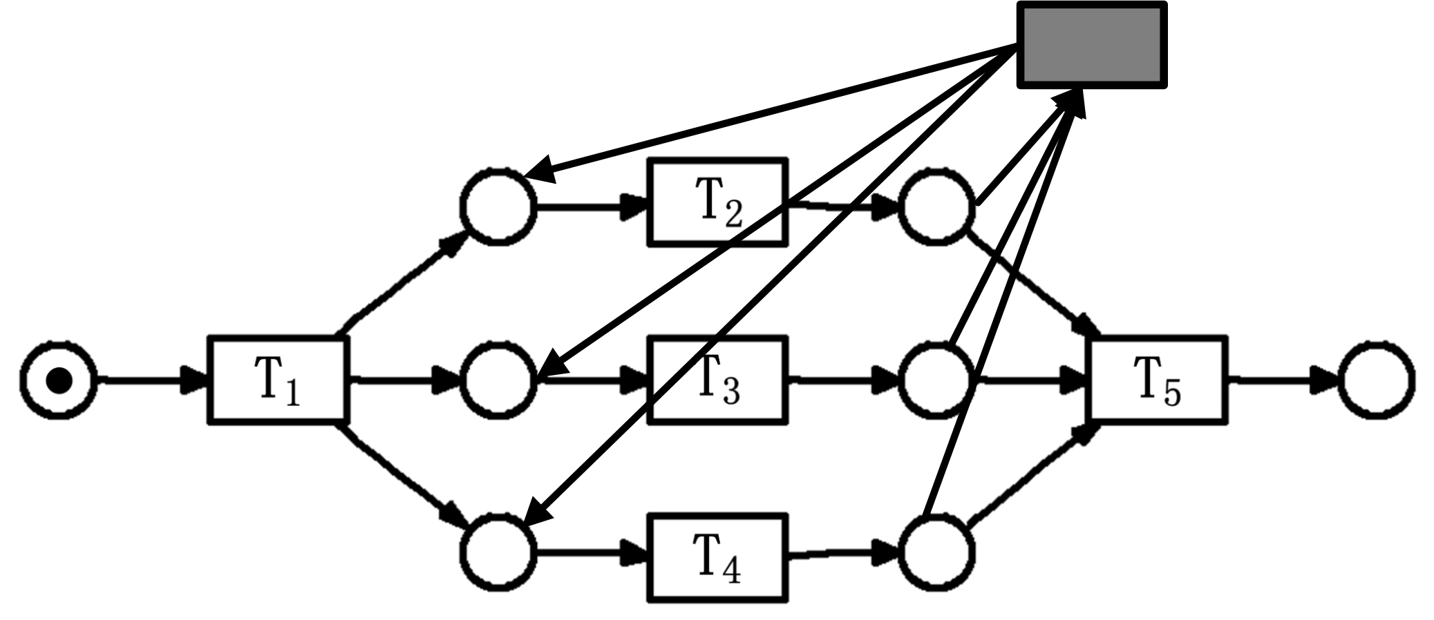
Figure 1: (a) and (b) (as well as (c) and (d)) have identical BPs but different behaviors

In the above figure, the nets in Fig. 1a and Fig. 1b have identical BP (we refer readers to the original work of [3] for definitions of BP), that is, for both nets we have T1{T2,T3,T4}T5subscript𝑇1subscript𝑇2subscript𝑇3subscript𝑇4subscript𝑇5T_{1}\rightarrow\{T_{2},T_{3},T_{4}\}\rightarrow T_{5} and {T2,T3,T4}subscript𝑇2subscript𝑇3subscript𝑇4\{T_{2},T_{3},T_{4}\} are mutually in parallel-to\parallel. Also, for both nets in Fig. 1c and Fig. 1d it holds T1T2T3subscript𝑇1subscript𝑇2subscript𝑇3T_{1}\rightarrow T_{2}\rightarrow T_{3}. However, these nets clearly have different behaviors. T2,T3,T4subscript𝑇2subscript𝑇3subscript𝑇4T_{2},T_{3},T_{4} in Fig. 1a form a parallel structure, whereas in Fig. 1b they form a loop.

Compared to BP, which describes the global ordering between transitions, Transition Adjacency Relation (TAR) captures more ‘local’ features among transitions that occur immediately one after another. This makes it a potential enhancement to BP based behavior description. For example, in Fig. 1a, T4subscript𝑇4T_{4} may occur immediately after T2subscript𝑇2T_{2} (denoted as T2<tarT4subscript𝑡𝑎𝑟subscript𝑇2subscript𝑇4T_{2}<_{tar}T_{4}), and T2subscript𝑇2T_{2} may also occur immediately after T4subscript𝑇4T_{4} (T4<tarT2subscript𝑡𝑎𝑟subscript𝑇4subscript𝑇2T_{4}<_{tar}T_{2}), but T4subscript𝑇4T_{4} cannot occur immediately after T2subscript𝑇2T_{2} in Fig. 1b. Moreover, T2subscript𝑇2T_{2} in Fig. 1d can be skipped whereas T2subscript𝑇2T_{2} in Fig. 1c cannot, which can be observed with TAR, as T3subscript𝑇3T_{3} may occur immediately after T1subscript𝑇1T_{1} (T1<tarT3subscript𝑡𝑎𝑟subscript𝑇1subscript𝑇3T_{1}<_{tar}T_{3}) in Fig. 1d but not in Fig. 1c.

As we have observed in the above examples, models with identical BP may have different TAR. Therefore, BP cannot be used to derive TAR even though unfolding-based BP computation has been addressed in [4], because we cannot directly rely on BP information to compute TAR (the vice-versa is also true, so we are not arguing that TAR is a superior representation than BP, but it is a potentially useful extension to BP). Nevertheless, the CFP structure built during BP computation is already available for re-use during TAR computation.

Admittedly, apart from TAR, arbitrarily many other relational semantics can be incorporated with BP to extend its expressive power, such as the reduced event structures proposed in [14]. However, the trade-off between simplicity (for both computation and human understanding) and more expressive power must be taken into account. In this sense, any additional relational semantics that bring more expressive power at smaller cost of complexity is considered more desirable. Moreover, since BP are generally computed by building the complete finite prefix (CFP) of unfolding [4], a preferable relational semantics for enhancement should be efficiently computable by re-using information from the CFP structure built previously.

As a consequence, we are motivated to put TAR’s computation in the context of unfolding to save the marginal cost and establish the potential of TAR as such a desirable addition to BP. This article explores unfolding based TAR/pTAR computation in three stages. First, we confirm that TAR computation can generally be reduced to the classic coverability problem and therefore solvable using the ‘co’ relations among conditions in the CFP , but the reduction of pTAR computation to coverability problems is not always trivial (Sect. 3). By re-using the causal information in the CFP more substantially, the computation of both TAR and pTAR can be further accelerated using a handful of derivation rules (Sect. 4). However, the incompleteness of unfolding information in CFP caused by cut-off events still restricts the applicability of these rules sometimes. Therefore, in Sect. 5, we describe our findings about a novel kind of finite extension of CFP, in which adequate information is preserved, so that TAR/pTAR can be derived from this extension completely using rules similar to those in Sect. 4.

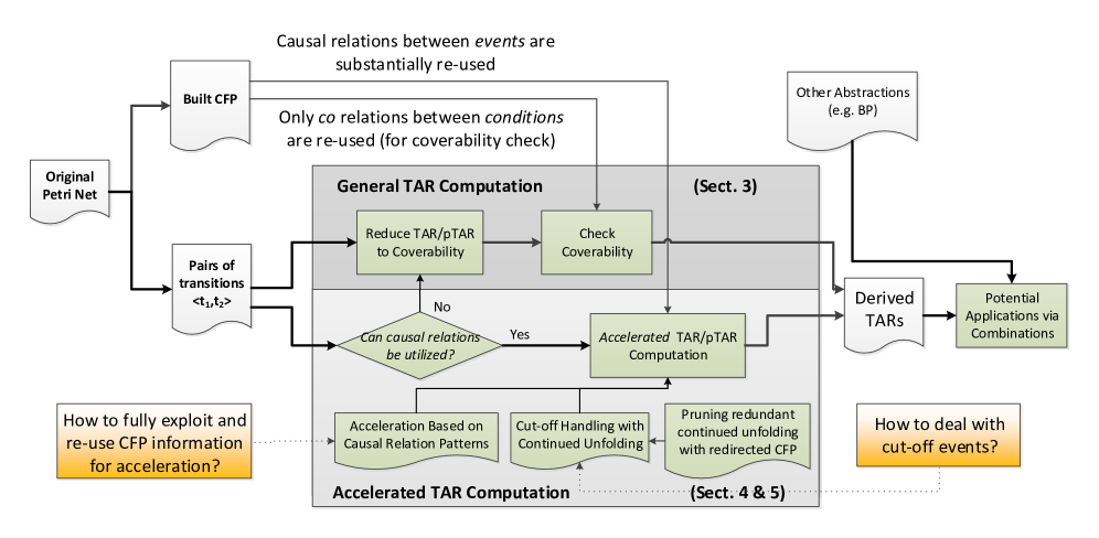
An overview of our work is summarized in Fig. 2. We set out to exploit all information available in CFP for TAR computation to the best of our knowledge, and achieved the leading performance among existing methods. With this work, we attempt to pave the way for further researches of the computation of TAR/pTAR and its application in business process behavior analysis, especially through combinations with other behavior abstractions such as BP.
Refer to caption
Figure 2: An overview of our research in unfolding-based TAR computation

This paper is an extended version of our previous work [15], but with significant amount of new contributions to the problem of transition adjacency relation (TAR) computation. A new type of cut-off criteria for constructing finite prefixes of Petri net unfolding has been provided in this paper to remove the necessity of costly coverability checking operation, which has been identified in our previous work [15] a major challenge to TAR computation. More in-depth proofs and experiments have been provided in this manuscript to make the proposed TAR/pTAR computation techniques more solid. Furthermore, we have provide additional business process model retrieval experiments in this version to demonstrate the necessity and application potential of combined usage of TAR and behavior profiles in this extended version.

The remaining of this paper (excepting Sect. 34, and 5) is organized as follows. Section 6 evaluates the TAR/pTAR computation performance on real-world data and the scalability of our algorithms. In Section 7, we show the effectiveness of the combination of TAR and BP by a concrete experiment on process model querying. Section 8 concludes our work.

2 Preliminary Concepts

We first recall the basic definitions on Petri net syntax and semantics [16].

Definition 2.1 (Petri net)

A Petri net is a triple N=(P,T,F)𝑁𝑃𝑇𝐹N=(P,T,F), where P and T are finite set of places and transitions respectively (PT=(P\cap T=\emptyset and PT)P\cup T\neq\emptyset), and F(P×T)(T×P)𝐹𝑃𝑇𝑇𝑃F\subseteq(P\times T)\cup(T\times P) is a set of arcs (flow relation). Denote X=PT𝑋𝑃𝑇X=P\cup T, for a node xX𝑥𝑋x\in X, x={yX|(y,x)F}\bullet x=\{y\in X|(y,x)\in F\}, x={yX|(x,y)F}x\bullet=\{y\in X|(x,y)\in F\}.

Definition 2.2 (Petri net semantics)

Let N=(P,T,F)𝑁𝑃𝑇𝐹N=(P,T,F) be a Petri net, then

  • M:P:𝑀𝑃M:P\rightarrow\mathbb{N} is a marking of N𝑁N, \mathbb{N} is the set of non-negative integers. 𝕄𝕄\mathbb{M} denotes all possible markings of N𝑁N. M(p)𝑀𝑝M(p) denotes the number of tokens in place p𝑝p.

  • A transition t is enabled in M𝑀M, iff pt:M(p)1\forall p\in\bullet t:M(p)\geq 1. If t is enabled at M𝑀M then it can be fired, and then a new marking Msuperscript𝑀M^{\prime} is reachable from M𝑀M by firing t, denoted by M𝑡M𝑡𝑀superscript𝑀M\xrightarrow{t}M^{\prime}, such that M=(M\t)tM^{\prime}=(M\backslash\bullet t)\cup t\bullet.

  • A net system is a pair S=(N,M0)𝑆𝑁subscript𝑀0S=(N,M_{0}), where N𝑁N is a net and M0subscript𝑀0M_{0} is the initial marking of N𝑁N.

  • A firing sequence σ=t1,,tn1𝜎subscript𝑡1subscript𝑡𝑛1\sigma=\langle t_{1},...,t_{n-1}\rangle leads N𝑁N from marking M1subscript𝑀1M_{1} to marking Mnsubscript𝑀𝑛M_{n} such that M1t1M2t2M3Mn1tn1Mnsubscript𝑡1subscript𝑀1subscript𝑀2subscript𝑡2subscript𝑀3subscript𝑀𝑛1subscript𝑡𝑛1subscript𝑀𝑛M_{1}\xrightarrow{t_{1}}M_{2}\xrightarrow{t_{2}}M_{3}...M_{n-1}\xrightarrow{t_{n-1}}M_{n}, also denoted as M1𝜎Mn𝜎subscript𝑀1subscript𝑀𝑛M_{1}\xrightarrow{\sigma}M_{n}. We use σ(i)𝜎𝑖\sigma(i) to denote the ithsuperscript𝑖𝑡i^{th} transition in sequence σ𝜎\sigma.

  • For a net system S(N,M0)𝑆𝑁subscript𝑀0S(N,M_{0}), M𝑀M is a reachable marking if from initial marking M0subscript𝑀0M_{0} there exists a firing sequence σ𝜎\sigma such that M0𝜎M𝜎subscript𝑀0𝑀M_{0}\xrightarrow{\sigma}M.

  • A net system is bounded if it has a finite number of reachable markings.

  • S(N,M0)𝑆𝑁subscript𝑀0S(N,M_{0}) is 1-safe iff for each reachable marking M𝑀M, M(p)𝑀𝑝absentM(p)\leq1 for every place p, and is free-choice iff t1,t2T:t1t2t1=t2\forall t_{1},t_{2}\in T:\bullet t_{1}\cap\bullet t_{2}\neq\emptyset\Rightarrow\bullet t_{1}=\bullet t_{2}.

The unfolding of a Petri net is derived from its related Occurrence Net, whose definition is based on the concepts of causal, conflict, and concurrency relations between Petri net nodes [17]. In a Petri net, two nodes x𝑥x and y𝑦y are in causal relation, denoted by x<y𝑥𝑦x<y, if the net contains a path with at least one arc leading from x𝑥x to y𝑦y. Furthermore, x𝑥x and y𝑦y are in conflict relation, denoted by x#y𝑥#𝑦x\#y, if the net contains two paths st1x1𝑠subscript𝑡1subscript𝑥1s\cdot t_{1}...\cdot x_{1} and st2x2𝑠subscript𝑡2subscript𝑥2s\cdot t_{2}...\cdot x_{2} starting at the same place s𝑠s, and such that t1t2subscript𝑡1subscript𝑡2t_{1}\neq t_{2}. Finally, x𝑥x and y𝑦y are in concurrency relation, denoted by x𝑥x co y𝑦y, if neither x<y𝑥𝑦x<y nor y<x𝑦𝑥y<x nor x#y𝑥#𝑦x\#y.

Definition 2.3 (Occurrence net)

An occurrence net is a net O=(C,E,G)𝑂𝐶𝐸𝐺O=(C,E,G), in which places are called conditions (C𝐶C), transitions are called events (E𝐸E), and:

  • O𝑂O is acyclic, or equivalently, the causal relation is a partial order.

  • cC:|c|1\forall c\in C:|\bullet c|\leq 1, and for all xCE𝑥𝐶𝐸x\in C\cup E it holds ¬(x#x)𝑥#𝑥\neg(x\#x) and the set {yCE|y<x}conditional-set𝑦𝐶𝐸𝑦𝑥\{y\in C\cup E|y<x\} is finite.

  • For an occurrence net O=(C,E,G)𝑂𝐶𝐸𝐺O=(C,E,G), Min(O)𝑀𝑖𝑛𝑂Min(O) denotes the set of minimal elements of CE𝐶𝐸C\cup E with respect to <<.

The relation between a net system S=(N,M0)𝑆𝑁subscript𝑀0S=(N,M_{0}) with N=(P,T,F)𝑁𝑃𝑇𝐹N=(P,T,F) and an occurrence net O=(C,E,G)𝑂𝐶𝐸𝐺O=(C,E,G) is defined as a homomorphism h:CEPT:𝐶𝐸𝑃𝑇h:C\cup E\longmapsto P\cup T such that h(C)P𝐶𝑃h(C)\subseteq P and h(E)T𝐸𝑇h(E)\subseteq T.

A branching process of S=(N,M0)𝑆𝑁subscript𝑀0S=(N,M_{0}) is a tuple π=(O,h)𝜋𝑂\pi=(O,h) with O=(C,E,G)𝑂𝐶𝐸𝐺O=(C,E,G) being an occurrence net and hh being a homomorphism from O𝑂O to S𝑆S. The maximal branching process of S𝑆S is called unfolding [17]. The unfolding of a net system can be truncated once all markings of the original net system and all enabled transitions are represented. This yields the complete finite prefix (abbr. CFP).

Definition 2.4 (Complete Finite Prefix)

Let S=(N,M0)𝑆𝑁subscript𝑀0S=(N,M_{0}) be a system and π=(O,h)𝜋𝑂\pi=(O,h) a branching process with N=(P,T,F)𝑁𝑃𝑇𝐹N=(P,T,F) and O=(C,E,G)𝑂𝐶𝐸𝐺O=(C,E,G).

  • A set of events EEsuperscript𝐸𝐸E^{\prime}\subseteq E is a configuration, iff e,fE:¬(e#f):for-all𝑒𝑓superscript𝐸𝑒#𝑓\forall e,f\in E^{\prime}:\neg(e\#f) and eE:f<efE:for-all𝑒superscript𝐸𝑓𝑒𝑓superscript𝐸\forall e\in E^{\prime}:f<e\Rightarrow f\in E^{\prime}. The local configuration [e]delimited-[]𝑒[e] for an event eE𝑒𝐸e\in E is defined as {xE|x<ex=e}conditional-set𝑥𝐸𝑥𝑒𝑥𝑒\{x\in E|x<e\vee x=e\}.

  • A set of conditions XC𝑋𝐶X\subseteq C is called co-set, iff for all distinct c1,c2Xsubscript𝑐1subscript𝑐2𝑋c_{1},c_{2}\in X it holds c1subscript𝑐1c_{1} co c2subscript𝑐2c_{2}. If Xsuperscript𝑋X^{\prime} is maximal w.r.t. set inclusion, it is called a cut. For a finite configuration Esuperscript𝐸E^{\prime}, Cut(E)=(Min(O)E)\ECut(E^{\prime})=(Min(O)\cup E^{\prime}\bullet)\backslash\bullet E^{\prime} is a cut, while h(Cut(E))𝐶𝑢𝑡superscript𝐸h(Cut(E^{\prime})) is a reachable marking of S𝑆S, denoted as Mark(E)𝑀𝑎𝑟𝑘superscript𝐸Mark(E^{\prime}), e.g. Mark([e])𝑀𝑎𝑟𝑘delimited-[]𝑒Mark([e]) is the set of places that are marked after all events in [e]delimited-[]𝑒[e] are fired.

  • An adequate order precedes\prec is a strict well-founded partial order on local configurations such that for two events e,fE𝑒𝑓𝐸e,f\in E, [e][f]delimited-[]𝑒delimited-[]𝑓[e]\subset[f] implies [e][f]precedesdelimited-[]𝑒delimited-[]𝑓[e]\prec[f].

  • An event e𝑒e is a cut-off event if there exists another event esuperscript𝑒e^{\prime} such that Mark([e])=Mark([e])𝑀𝑎𝑟𝑘delimited-[]𝑒𝑀𝑎𝑟𝑘delimited-[]superscript𝑒Mark([e])=Mark([e^{\prime}]) and [e][e]precedesdelimited-[]superscript𝑒delimited-[]𝑒[e^{\prime}]\prec[e]. esuperscript𝑒e^{\prime} is the corresponding event of e𝑒e, denoted as e=corr(e)superscript𝑒𝑐𝑜𝑟𝑟𝑒e^{\prime}=corr(e).

  • A complete finite prefix (CFP) is the greatest backward-closed subnet of a branching process containing no events after any cut-off event.

Example 2.1
Refer to caption
(a)
Refer to caption
(b)
Refer to caption
(c)
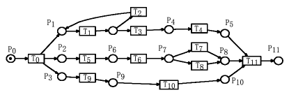
Figure 3: CFP as a more compact representation for Petri net behavior analysis

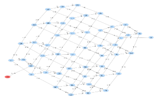
Fig. 3a, 3b and 3c illustrate a Petri net, its related reachability graph and CFP respectively (Fig. 3b is not supposed to be readable, only intended to illustrate the complexity of the reachability graph). Although there are multiple solutions as Fig. 3a’s CFP, we only show one of them here for simplicity. In this paper, we name each event with its related transition name, which is followed by ‘-’ and then its order of appearance in the CFP. For example, in Fig. 3c, T8-10subscript𝑇8-10T_{8}\mbox{-}10 is an event that maps to T8subscript𝑇8T_{8} of the original net (h(T8-10)=T8subscript𝑇8-10subscript𝑇8h(T_{8}\mbox{-}10)=T_{8}), and it is the tenth event constructed in the CFP. In Fig. 3c, [T8-10]={T0-1,T5-4,T6-8,T8-10}delimited-[]subscript𝑇8-10subscript𝑇0-1subscript𝑇5-4subscript𝑇6-8subscript𝑇8-10[T_{8}\mbox{-}10]=\{T_{0}\mbox{-}1,T_{5}\mbox{-}4,T_{6}\mbox{-}8,T_{8}\mbox{-}10\}, [T7-11]={T0-1,T5-4,T6-8,T7-11}delimited-[]subscript𝑇7-11subscript𝑇0-1subscript𝑇5-4subscript𝑇6-8subscript𝑇7-11[T_{7}\mbox{-}11]=\{T_{0}\mbox{-}1,T_{5}\mbox{-}4,T_{6}\mbox{-}8,T_{7}\mbox{-}11\}, and Mark([T8-10])𝑀𝑎𝑟𝑘delimited-[]subscript𝑇8-10Mark([T_{8}\mbox{-}10])=Mark([T7-11])absent𝑀𝑎𝑟𝑘delimited-[]subscript𝑇7-11=Mark([T_{7}\mbox{-}11])={P1,P3,P8}absentsubscript𝑃1subscript𝑃3subscript𝑃8=\{P_{1},P_{3},P_{8}\}, thus T7-11subscript𝑇7-11T_{7}\mbox{-}11 is a cut-off event, and T8-10subscript𝑇8-10T_{8}\mbox{-}10 is its corresponding event. T2-6subscript𝑇2-6T_{2}\mbox{-}6 is a cut-off event caused by looping, whose corresponding event is T0-1subscript𝑇0-1T_{0}\mbox{-}1.

A reachability graph (RG) is prone to encounter state-explosions with concurrent behaviors (because it enumerates all possible execution traces), whereas the CFP of a Petri net only ‘outlines’ the net’s behavior and is much more compact, as illustrated in Fig. 3b and 3c.

In this paper, we adopt Esparza’s algorithm [17] for CFP construction, which can generate more compact CFPs compared to the original CFP construction technique. We also refer readers to [17] for more examples on unfolding.

Let us now present the definition of Transition Adjacency Relation (TAR) and Projected Transition Adjacency Relation (pTAR):

Definition 2.5 (Transition Adjacency Relation)

Let S=(N,M0)𝑆𝑁subscript𝑀0S=(N,M_{0}) be a net system. Let t1,t2subscript𝑡1subscript𝑡2t_{1},t_{2} be two transitions of S. We say that t1,t2subscript𝑡1subscript𝑡2t_{1},t_{2} are in Transition Adjacency Relation, denoted as t1<tart2subscript𝑡𝑎𝑟subscript𝑡1subscript𝑡2t_{1}<_{tar}t_{2}, if there exist a reachable marking Mssubscript𝑀𝑠M_{s} of S𝑆S, where t1subscript𝑡1t_{1} is enabled, and Mst1Mssubscript𝑡1subscript𝑀𝑠superscriptsubscript𝑀𝑠M_{s}\xrightarrow{t_{1}}M_{s}^{\prime}, such that t2subscript𝑡2t_{2} is enabled at Mssuperscriptsubscript𝑀𝑠M_{s}^{\prime}.

Definition 2.6 (Projected Transition Adjacency Relation)

Let t1,t2subscript𝑡1subscript𝑡2t_{1},t_{2} be two non-silent transitions of a net system S(N,M0)𝑆𝑁subscript𝑀0S(N,M_{0}). We say that t1subscript𝑡1t_{1} and t2subscript𝑡2t_{2} are in projected Transition Adjacency Relation (pTAR), denoted as t1<ptart2subscript𝑝𝑡𝑎𝑟subscript𝑡1subscript𝑡2t_{1}<_{ptar}t_{2} iff from M0subscript𝑀0M_{0} a sequence σ𝜎\sigma can be fired such that σ(i)=t1,σ(j)=t2formulae-sequence𝜎𝑖subscript𝑡1𝜎𝑗subscript𝑡2\sigma(i)=t_{1},\sigma(j)=t_{2} for some 1i<j1𝑖𝑗1\leq i<j and σ(k)𝜎𝑘\sigma(k) are silent transitions for all i<k<j𝑖𝑘𝑗i<k<j.

Figure 4: Illustration of TAR and pTAR
Refer to caption

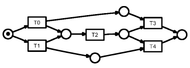
Intuitively, TAR says ‘some pair of transitions can occur immediately one after another’, and pTAR (Projected TAR, or Silent TAR) says ‘some pair of transitions can occur immediately one after another, if the silent transitions occurring between them are neglected’. For example, in Fig. 4, T1subscript𝑇1T_{1} and T2subscript𝑇2T_{2}, T2subscript𝑇2T_{2} and T3subscript𝑇3T_{3} are in TAR, denoted as T1<tarT2,T2<tarT3formulae-sequencesubscript𝑡𝑎𝑟subscript𝑇1subscript𝑇2subscript𝑡𝑎𝑟subscript𝑇2subscript𝑇3T_{1}<_{tar}T_{2},T_{2}<_{tar}T_{3}, and T1subscript𝑇1T_{1} are in pTAR with T3subscript𝑇3T_{3} (T1<ptarT3subscript𝑝𝑡𝑎𝑟subscript𝑇1subscript𝑇3T_{1}<_{ptar}T_{3}), as we can skip T2subscript𝑇2T_{2} by firing the silent transition I2subscript𝐼2I_{2}. The definition is equivalent with the the one in [2], where projected transitions are treated as non-silent transitions and the rest as silent transitions.

3 Baseline Approach of TAR Computation from CFP

The CFP of a Petri net contains various information that we can exploit for TAR computation. In this section, we look at how to exploit the co𝑐𝑜co relations between conditions in CFP, by reducing TAR computation to coverability checking.

3.1 Reduction of TAR Computation to Coverability Problem

First we show that the computation of TAR can be reduced to the classic coverability problem, that is, checking if a certain set of places can be ‘covered’ by some reachable marking of a Petri net. We prove this as follows.

Theorem 3.1

For two transitions t1,t2subscript𝑡1subscript𝑡2t_{1},t_{2} in a bounded net system: t1<tart2(t2\t1)t1t_{1}<_{tar}t_{2}\Leftrightarrow(\bullet t_{2}\backslash t_{1}\bullet)\cup\bullet t_{1} is coverable.

Proof:

By definition of TAR, we have t1<tart2subscript𝑡𝑎𝑟subscript𝑡1subscript𝑡2t_{1}<_{tar}t_{2} iff there exists a reachable marking M:Mt1Mt2M′′:𝑀subscript𝑡1𝑀superscript𝑀subscript𝑡2superscript𝑀′′M:M\xrightarrow{t_{1}}M^{\prime}\xrightarrow{t_{2}}M^{\prime\prime}. Then Mt1Mt2M′′subscript𝑡1𝑀superscript𝑀subscript𝑡2superscript𝑀′′M\xrightarrow{t_{1}}M^{\prime}\xrightarrow{t_{2}}M^{\prime\prime} holds if and only t2M\bullet t_{2}\subseteq M^{\prime} and t1M\bullet t_{1}\subseteq M, which holds if and only if (t2\t1)t1M(\bullet t_{2}\backslash t_{1}\bullet)\cup\bullet t_{1}\subseteq M.

Since M𝑀M is a reachable marking of S𝑆S, by the above reasoning we have that t1<tart2(t2\t1)t1t_{1}<_{tar}t_{2}\Leftrightarrow(\bullet t_{2}\backslash t_{1}\bullet)\cup\bullet t_{1} is coverable. ∎

In CFP, a coverable marking of the net system corresponds with a set of conditions that are mutually in co𝑐𝑜co relations (i.e., a co𝑐𝑜co-set) [14]. Consequently, the coverability problem can be solved efficiently based on the co𝑐𝑜co relations between conditions in CFPs using SAT solvers [18]. Therefore, a general algorithm of unfolding-based TAR computation can be given as Algorithm 1.

Algorithm 1 General TAR Derivation Using CFP (GENERAL)
1:function GENERAL(S,π𝑆𝜋S,\pi)
2:     TAR𝑇𝐴𝑅TAR\leftarrow\emptyset
3:     for each t1,t2Ssubscript𝑡1subscript𝑡2𝑆t_{1},t_{2}\in S do
4:     Check coverability of (t2\t1)t1(\bullet t_{2}\backslash t_{1}\bullet)\cup\bullet t_{1} based on π𝜋\pi using SAT solvers
5:     if (t2\t1)t1(\bullet t_{2}\backslash t_{1}\bullet)\cup\bullet t_{1} is coverable then TARTAR{t1,t2}𝑇𝐴𝑅𝑇𝐴𝑅subscript𝑡1subscript𝑡2TAR\leftarrow TAR\cup\{\langle t_{1},t_{2}\rangle\}
6:     return TAR𝑇𝐴𝑅TAR
7:end function

3.2 Reduction of pTAR to Coverability And Its Non-triviality

Unlike the original TAR, the checking of projected TARs (pTARs) between a given pair of transitions t1,t2subscript𝑡1subscript𝑡2t_{1},t_{2} cannot be trivially reduced to coverability problem. Unlike in Thm. 3.1, where t2subscript𝑡2t_{2} can be fired immediately after t1subscript𝑡1t_{1}, it is probable that after firing t1subscript𝑡1t_{1}, a sequence of silent transitions have to be fired before t2subscript𝑡2t_{2} is fired. In this case, suppose we want to reduce the checking of pTAR to the coverability problem, we need to know the firing sequence between t1subscript𝑡1t_{1} and t2subscript𝑡2t_{2}. In other words, we need to determine a sequence σ=ti1,,tik𝜎subscript𝑡subscript𝑖1subscript𝑡subscript𝑖𝑘\sigma=\langle t_{i_{1}},...,t_{i_{k}}\rangle such that there exists a reachable marking M𝑀M such that Mt1M1ti1M2ti2MktikMk+1t2Mk+2subscript𝑡1𝑀subscript𝑀1subscript𝑡subscript𝑖1subscript𝑀2subscript𝑡subscript𝑖2subscript𝑀𝑘subscript𝑡subscript𝑖𝑘subscript𝑀𝑘1subscript𝑡2subscript𝑀𝑘2M\xrightarrow{t_{1}}M_{1}\xrightarrow{t_{i_{1}}}M_{2}\xrightarrow{t_{i_{2}}}...M_{k}\xrightarrow{t_{i_{k}}}M_{k+1}\xrightarrow{t_{2}}M_{k+2}. By the same reasoning in Thm. 3.1, Pk=(t2\tik)tikP_{k}=(\bullet t_{2}\backslash t_{i_{k}}\bullet)\cup\bullet t_{i_{k}} must be covered by Mksubscript𝑀𝑘M_{k}, Pk1=(Pk\tik1)tik1P_{k-1}=(P_{k}\backslash t_{i_{k-1}}\bullet)\cup\bullet t_{i_{k-1}} must be covered by Mk1subscript𝑀𝑘1M_{k-1}, etc. So the pTAR checking between t1subscript𝑡1t_{1} and t2subscript𝑡2t_{2}, with respect to some σ𝜎\sigma, can be reduced to the coverability checking of P1=((((t2\tik)tik)\tik1)tik1\t1)t1P_{1}=(...(((\bullet t_{2}\backslash t_{i_{k}}\bullet)\cup\bullet t_{i_{k}})\backslash t_{i_{k-1}}\bullet)\cup\bullet t_{i_{k-1}}...\backslash t_{1}\bullet)\cup\bullet t_{1}.

However, although pTAR checking can be reduced to coverability problem in this way, the determination of a concrete σ𝜎\sigma, which is the prerequisite for such reduction, is non-trivial, because there can be numerous possible firing paths between a pair of transitions.

4 Exploiting More CFP Relations for Accelerations

Although being complete and correct, Algorithm 1 includes the costly operation of coverability checking, and pTAR checking can not be reduced to coverability problem at trivial costs.

In Algorithm 1, since TAR computation is reduced to coverability checking, only co𝑐𝑜co relations between conditions are used, and the rest of the CFP (causal relations and co𝑐𝑜co between events) are not utilized. We believe these unused information will be exactly the keys to accelerate TAR computation. By dividing the TAR cases into the following two categories, we may construct more connections between TAR and information in CFP:
(1)t1t2=(1)~{}t_{1}\bullet\cap\bullet t_{2}=\emptyset (non-consecutive),
(2)t1t2(2)~{}t_{1}\bullet\cap\bullet t_{2}\neq\emptyset (consecutive).

In case of (1)t1t2=(1)t_{1}\bullet\cap\bullet t_{2}=\emptyset, since t1subscript𝑡1t_{1} and t2subscript𝑡2t_{2} in this case are non-consecutive, we have the intuition that TARs between non-consecutive transitions corresponds to co𝑐𝑜co relations in CFP. Fortunately, we find that such TARs can always be identified in CFP as co𝑐𝑜co relations because of the following useful property of CFP.

Property 4.1

For every reachable marking M𝑀M of a Petri net system S𝑆S, there exists a configuration 𝒞𝒞\mathcal{C} in a corresponding CFP π𝜋\pi of S𝑆S such that Mark(𝒞)=M𝑀𝑎𝑟𝑘𝒞𝑀Mark(\mathcal{C})=M and 𝒞𝒞\mathcal{C} does not contain any cut-off event.

Proof:

Given a configuration 𝒞𝒞\mathcal{C}, we denote by 𝒞Edirect-sum𝒞𝐸\mathcal{C}\oplus E the fact that 𝒞E𝒞𝐸\mathcal{C}\cup E is a configuration such that 𝒞E=𝒞𝐸\mathcal{C}\cap E=\emptyset. We say that 𝒞Edirect-sum𝒞𝐸\mathcal{C}\oplus E is an extension of 𝒞𝒞\mathcal{C}, and that E𝐸E is a suffix of 𝒞𝒞\mathcal{C}. Let 𝒞1subscript𝒞1\mathcal{C}_{1} be a configuration in the unfolding of S𝑆S such that Mark(𝒞1subscript𝒞1\mathcal{C}_{1})=M𝑀M. Suppose 𝒞1subscript𝒞1\mathcal{C}_{1} contains some cut-off event e1 and that 𝒞1subscript𝒞1\mathcal{C}_{1} = [e1subscript𝑒1e_{1}]E1direct-sumsubscript𝐸1\oplus E_{1} for some set of events E1subscript𝐸1E_{1}. By the definition of a cut-off event, there exists a local configuration [e2subscript𝑒2e_{2}] such that [e2subscript𝑒2e_{2}] precedes\prec [e1subscript𝑒1e_{1}] and Mark([e2subscript𝑒2e_{2}]) = Mark([e1subscript𝑒1e_{1}]).According to the original theory of Petri net unfolding, there is a set of events isomorphic (corresponding to the same set of transitions) with E1subscript𝐸1E_{1}, denoted as I12(E1)superscriptsubscript𝐼12subscript𝐸1I_{1}^{2}(E_{1}), such that Mark([e2subscript𝑒2e_{2}]I12(E1))=\oplus I_{1}^{2}(E_{1}))=Mark(𝒞1subscript𝒞1\mathcal{C}_{1}). Consider the configuration 𝒞2subscript𝒞2\mathcal{C}_{2} = [e2subscript𝑒2e_{2}]I12(E1)direct-sumsuperscriptsubscript𝐼12subscript𝐸1\oplus I_{1}^{2}(E_{1}). Since precedes\prec is preserved by finite extensions, we have 𝒞2𝒞1precedessubscript𝒞2subscript𝒞1\mathcal{C}_{2}\prec\mathcal{C}_{1}. If 𝒞2subscript𝒞2\mathcal{C}_{2} still contains any cut-off event, we can repeat the procedure and find a configuration 𝒞3subscript𝒞3\mathcal{C}_{3} such that 𝒞3𝒞2precedessubscript𝒞3subscript𝒞2\mathcal{C}_{3}\prec\mathcal{C}_{2} and that Mark(𝒞3subscript𝒞3\mathcal{C}_{3})=Mark(𝒞2subscript𝒞2\mathcal{C}_{2}). The procedure cannot be iterated infinitely often because precedes\prec is well-founded. Therefore, it terminates in a configuration 𝒞𝒞\mathcal{C} in CFP which does not contain any cut-off event and Mark(𝒞𝒞\mathcal{C}) = M𝑀M. ∎

Theorem 4.1

Let S𝑆S be a bounded net system and π=(O,h)𝜋𝑂\pi=(O,h) its CFP, where O=(C,E,G)𝑂𝐶𝐸𝐺O=(C,E,G) . Let t1,t2subscript𝑡1subscript𝑡2t_{1},t_{2} be two transitions of S𝑆S. When t1t2=t_{1}\bullet\cap\bullet t_{2}=\emptyset, we have t1<tart2e1,e2E:e1subscript𝑡𝑎𝑟subscript𝑡1subscript𝑡2subscript𝑒1subscript𝑒2𝐸:subscript𝑒1t_{1}<_{tar}t_{2}\Leftrightarrow\exists e_{1},e_{2}\in E:e_{1} co e2subscript𝑒2e_{2}, h(e1)=t1,h(e2)=t2formulae-sequencesubscript𝑒1subscript𝑡1subscript𝑒2subscript𝑡2h(e_{1})=t_{1},h(e_{2})=t_{2}.

Proof:

(\Rightarrow) By t1<tart2subscript𝑡𝑎𝑟subscript𝑡1subscript𝑡2t_{1}<_{tar}t_{2}, there are markings Ms,Mssubscript𝑀𝑠superscriptsubscript𝑀𝑠M_{s},M_{s}^{\prime} in S𝑆S such that Mst1Mssubscript𝑡1subscript𝑀𝑠superscriptsubscript𝑀𝑠M_{s}\xrightarrow{t_{1}}M_{s}^{\prime}, and that t2subscript𝑡2t_{2} is enabled at Mssuperscriptsubscript𝑀𝑠M_{s}^{\prime}. Since t1t2=t_{1}\bullet\cap\bullet t_{2}=\emptyset, we know both t1absentsubscript𝑡1\bullet t_{1} and t2absentsubscript𝑡2\bullet t_{2} have tokens in them at Mssubscript𝑀𝑠M_{s}. By Property 4.1, there exists a configuration C𝐶C in π𝜋\pi such that C𝐶C does not contain any cut-off event and that Mark(C)=Ms𝑀𝑎𝑟𝑘𝐶subscript𝑀𝑠Mark(C)=M_{s}. Therefore X1Cut(C):h(X1)=t1\exists X_{1}\subseteq Cut(C):h(X_{1})=\bullet t_{1}. Since C𝐶C does not contain cut-off events, there exists in π𝜋\pi an event e1:h(e1)=t1,e1=X1e_{1}:h(e_{1})=t_{1},\bullet e_{1}=X_{1}. Similarly, because t2subscript𝑡2t_{2} is enabled at Mssuperscriptsubscript𝑀𝑠M_{s}^{\prime}, e2π:h(e2)=t2,e2=X2Cut(C)\exists e_{2}\in\pi:h(e_{2})=t_{2},\bullet e_{2}=X_{2}\subseteq Cut(C) and X1X2=subscript𝑋1subscript𝑋2X_{1}\cap X_{2}=\emptyset. Therefore, it holds that e1e2not-less-thansubscript𝑒1subscript𝑒2e_{1}\not<e_{2} and ¬(e1#e2)subscript𝑒1#subscript𝑒2\neg(e_{1}\#e_{2}), and consequently, e1subscript𝑒1e_{1} co𝑐𝑜co e2subscript𝑒2e_{2}. (\Leftarrow) For some e1,e2E:e1:subscript𝑒1subscript𝑒2𝐸subscript𝑒1e_{1},e_{2}\in E:e_{1} co e2subscript𝑒2e_{2}, h(e1)=t1,h(e2)=t2formulae-sequencesubscript𝑒1subscript𝑡1subscript𝑒2subscript𝑡2h(e_{1})=t_{1},h(e_{2})=t_{2}, we know both e1absentsubscript𝑒1\bullet e_{1} and e2absentsubscript𝑒2\bullet e_{2} are co-set and c1e1,c2e2:c1\forall c_{1}\in\bullet e_{1},c_{2}\in\bullet e_{2}:c_{1} co c2subscript𝑐2c_{2}. Therefore e1e2=\bullet e_{1}\cap\bullet e_{2}=\emptyset and e1e2\bullet e_{1}\cup\bullet e_{2} is a co-set, so there exists a configuration C𝐶C in π𝜋\pi such that e1e2Cut(C)\bullet e_{1}\cup\bullet e_{2}\subseteq Cut(C). As h(e1)=t1h(\bullet e_{1})=\bullet t_{1} and h(e2)=t2h(\bullet e_{2})=\bullet t_{2}, both t1,t2subscript𝑡1subscript𝑡2t_{1},t_{2} are enabled at Mark(C)𝑀𝑎𝑟𝑘𝐶Mark(C). And after t1subscript𝑡1t_{1} is fired, t2subscript𝑡2t_{2} is still enabled (because e1e2=\bullet e_{1}\cap\bullet e_{2}=\emptyset). Therefore we have t1<tart2subscript𝑡𝑎𝑟subscript𝑡1subscript𝑡2t_{1}<_{tar}t_{2}. ∎

Now we consider the case of (2)t1t2(2)t_{1}\bullet\cap\bullet t_{2}\neq\emptyset. To solve this case, we introduce the concept of Max-Event Set.

Definition 4.1 (Max-Event Set)

Let E0subscript𝐸0E_{0} be a subset of the events in a CFP. We call the set of maximal events in E0subscript𝐸0E_{0} with respect to causal relation as its max-event set, denoted as Max(E0)={eE0|eE0:ee}𝑀𝑎𝑥subscript𝐸0conditional-set𝑒subscript𝐸0:for-allsuperscript𝑒subscript𝐸0not-less-than𝑒superscript𝑒Max(E_{0})=\{e\in E_{0}|\forall e^{\prime}\in E_{0}:e\not<e^{\prime}\}.

Given this definition, we have discovered the following results (see [19]).

Lemma 4.1

Let 𝒞𝒞\mathcal{C} be a configuration. Let Max(𝒞)={em1,,emk}𝑀𝑎𝑥𝒞subscript𝑒subscript𝑚1subscript𝑒subscript𝑚𝑘Max(\mathcal{C})=\{e_{m_{1}},...,e_{m_{k}}\}. Then

  • (1)

    𝒞\{e}\𝒞𝑒\mathcal{C}\backslash\{e\} is a configuration if and only if eMax(𝒞)𝑒𝑀𝑎𝑥𝒞e\in Max(\mathcal{C}).

  • (2)

    [em1][emk]=𝒞delimited-[]subscript𝑒subscript𝑚1delimited-[]subscript𝑒subscript𝑚𝑘𝒞[e_{m_{1}}]\cup...\cup[e_{m_{k}}]=\mathcal{C}.

Lemma 4.2

Let X𝑋X be a co-set in a CFP. Let Max(X)={em1,,emk}Max(\bullet X)=\{e_{m_{1}},...,e_{m_{k}}\}. Then 𝒞=[em1][emk]𝒞delimited-[]subscript𝑒subscript𝑚1delimited-[]subscript𝑒subscript𝑚𝑘\mathcal{C}=[e_{m_{1}}]\cup...\cup[e_{m_{k}}] is a configuration, and XCut(𝒞)𝑋𝐶𝑢𝑡𝒞X\subseteq Cut(\mathcal{C}), Max(𝒞)=Max(X)Max(\mathcal{C})=Max(\bullet X).

Lemma 4.3

eMax(𝒞)eCut(𝒞\{e})e\in Max(\mathcal{C})\Rightarrow\bullet e\subseteq Cut(\mathcal{C}\backslash\{e\}).

In case (2), when t1t2t_{1}\bullet\cap\bullet t_{2}\neq\emptyset, we capture the intuition of ‘non-blocking’ by introducing the following concept of Max-Event Adjacent (MEA).

Definition 4.2 (Max-Event Adjacent)

For two events e1subscript𝑒1e_{1} and e2subscript𝑒2e_{2} in a CFP such that e1<e2subscript𝑒1subscript𝑒2e_{1}<e_{2}, e1subscript𝑒1e_{1} is said to be Max-Event Adjacent (MEA) with e2subscript𝑒2e_{2}, denoted as e1e2subscript𝑒1subscript𝑒2e_{1}\triangleright e_{2}, iff e1Max((e2))e_{1}\in Max(\bullet(\bullet e_{2})). e1e2subscript𝑒1subscript𝑒2e_{1}\triangleright e_{2} can be equivalently defined as ce1:c<e2ce2\forall c\in e_{1}\bullet:c<e_{2}\Rightarrow c\in\bullet e_{2} (more convenient and efficient for implementation).

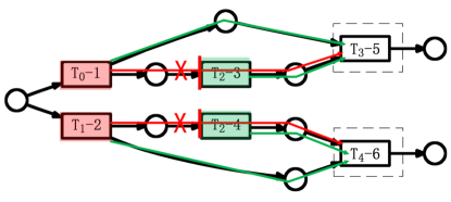
Intuitively, e1e2subscript𝑒1subscript𝑒2e_{1}\triangleright e_{2} means e1subscript𝑒1e_{1} is directly connected to e2subscript𝑒2e_{2}, but with an additional restriction that no third event ‘blocks’ any path between them. For example, in Fig. 5b, which shows the CFP of the net in Fig. 5a, we have (T3-5)={T0-1,T2-3}\bullet(\bullet T_{3}\mbox{-}5)=\{T_{0}\mbox{-}1,T_{2}\mbox{-}3\}, but only T2-3subscript𝑇2-3T_{2}\mbox{-}3 is MEA with T3-5subscript𝑇3-5T_{3}\mbox{-}5. T0-1subscript𝑇0-1T_{0}\mbox{-}1 is not MEA with T3-5subscript𝑇3-5T_{3}\mbox{-}5 because T0-1<T2-3subscript𝑇0-1subscript𝑇2-3T_{0}\mbox{-}1<T_{2}\mbox{-}3 and consequently T0-1Max((T3-5T_{0}\mbox{-}1\not\in Max(\bullet(\bullet T_{3}\mbox{-}5)) (intuitively, T2-3subscript𝑇2-3T_{2}\mbox{-}3 ‘blocks’ one of the paths between T0-1subscript𝑇0-1T_{0}\mbox{-}1 and T3-5subscript𝑇3-5T_{3}\mbox{-}5). Likewise, we have T2-4T4-6subscript𝑇2-4subscript𝑇4-6T_{2}\mbox{-}4\triangleright T_{4}\mbox{-}6 and ¬(T1-2T4-6)subscript𝑇1-2subscript𝑇4-6\neg(T_{1}\mbox{-}2\triangleright T_{4}\mbox{-}6).

MEA (\triangleright) is a sufficient condition to detect TARs in case (2), as we can prove using Lemma 4.1 and Lemma 4.3 that for any bounded Petri net’s CFP:

Theorem 4.2

e1e2h(e1)<tarh(e2)subscript𝑒1subscript𝑒2subscript𝑒1subscript𝑡𝑎𝑟subscript𝑒2e_{1}\triangleright e_{2}\Rightarrow h(e_{1})<_{tar}h(e_{2}).

Proof:

Let 𝒞=[e2]𝒞delimited-[]subscript𝑒2\mathcal{C}=[e_{2}]. By definition of local configuration, Max([e2])={e2}𝑀𝑎𝑥delimited-[]subscript𝑒2subscript𝑒2Max([e_{2}])=\{e_{2}\}. Therefore, by Lemma 4.1, 𝒞=𝒞\{e2}superscript𝒞\𝒞subscript𝑒2\mathcal{C^{\prime}}=\mathcal{C}\backslash\{e_{2}\} is a configuration, and by Lemma 4.3 we have: (a) e2Cut(𝒞).\bullet e_{2}\subseteq Cut(\mathcal{C^{\prime}}).

Moreover, it is easy to prove that Max([e2]\{e2})(e2)Max([e_{2}]\backslash\{e_{2}\})\subseteq\bullet(\bullet e_{2}). From e1e2subscript𝑒1subscript𝑒2e_{1}\triangleright e_{2}, we know e1Max((e2))e_{1}\in Max(\bullet(\bullet e_{2})), and therefore e1Max([e2]\{e2})=Max(𝒞)subscript𝑒1𝑀𝑎𝑥\delimited-[]subscript𝑒2subscript𝑒2𝑀𝑎𝑥superscript𝒞e_{1}\in Max([e_{2}]\backslash\{e_{2}\})=Max(\mathcal{C^{\prime}}). Consequently 𝒞′′=𝒞\{e1}superscript𝒞′′\superscript𝒞subscript𝑒1\mathcal{C^{\prime\prime}}=\mathcal{C^{\prime}}\backslash\{e_{1}\} is also a configuration. And by Lemma 4.3 it holds that: (b) e1Cut(𝒞′′).\bullet e_{1}\subseteq Cut(\mathcal{C^{\prime\prime}}).

Let the marking of π𝜋\pi corresponding to Cut(𝒞′′),Cut(𝒞)𝐶𝑢𝑡superscript𝒞′′𝐶𝑢𝑡superscript𝒞Cut(\mathcal{C^{\prime\prime}}),Cut(\mathcal{C^{\prime}}) and Cut(𝒞)𝐶𝑢𝑡𝒞Cut(\mathcal{C}) be denoted as M1,M1,M2subscript𝑀1superscriptsubscript𝑀1subscript𝑀2M_{1},M_{1}^{\prime},M_{2} respectively. By (a) and (b), it holds that M1e1M1e2M2subscript𝑒1subscript𝑀1superscriptsubscript𝑀1subscript𝑒2subscript𝑀2M_{1}\xrightarrow{e_{1}}M_{1}^{\prime}\xrightarrow{e_{2}}M_{2} and therefore h(e1)<tarh(e2)subscript𝑡𝑎𝑟subscript𝑒1subscript𝑒2h(e_{1})<_{tar}h(e_{2}). ∎

Refer to caption
(a)
Refer to caption
(b)
Refer to caption
(c)
Refer to caption
(d)
Figure 5: Applying Max-Event Adjacent Structure for TAR Derivation

However, MEA based TAR checking requires that the whole MEA structure is preserved in the CFP. In Fig. 5d, as T4-5subscript𝑇4-5T_{4}\mbox{-}5 is a cut-off event, Thm. 4.2 cannot be directly applied. To deal with such cases, we provide the following result:

Theorem 4.3

Let π𝜋\pi be the CFP of a bounded net system. Let e1subscript𝑒1e_{1} be a cut-off event and e1superscriptsubscript𝑒1e_{1}^{\prime} its corresponding event of π𝜋\pi and h(e1)=h(e1)h(e_{1}\bullet)=h(e_{1}^{\prime}\bullet). Then e1e2h(e1)<tarh(e2)superscriptsubscript𝑒1subscript𝑒2subscript𝑒1subscript𝑡𝑎𝑟subscript𝑒2e_{1}^{\prime}\triangleright e_{2}\Rightarrow h(e_{1})<_{tar}h(e_{2}).

Proof:

By e1e2superscriptsubscript𝑒1subscript𝑒2e_{1}^{\prime}\triangleright e_{2}, we know that e1Max((e2))e_{1}^{\prime}\in Max(\bullet(\bullet e_{2})), and therefore e1<e2superscriptsubscript𝑒1subscript𝑒2e_{1}^{\prime}<e_{2} and [e1][e2]\{e2}delimited-[]superscriptsubscript𝑒1\delimited-[]subscript𝑒2subscript𝑒2[e_{1}^{\prime}]\subseteq[e_{2}]\backslash\{e_{2}\}. By Lemma 4.3, we can construct a sequence of events g1,g2,,gksubscript𝑔1subscript𝑔2subscript𝑔𝑘g_{1},g_{2},...,g_{k} such that [e1]=[e2]\{e2}\{gk}\{gk1}\\{g1}delimited-[]superscriptsubscript𝑒1\delimited-[]subscript𝑒2subscript𝑒2subscript𝑔𝑘subscript𝑔𝑘1subscript𝑔1[e_{1}^{\prime}]=[e_{2}]\backslash\{e_{2}\}\backslash\{g_{k}\}\backslash\{g_{k-1}\}\backslash...\backslash\{g_{1}\}. Let h(g1),,h(gk)subscript𝑔1subscript𝑔𝑘h(g_{1}),...,h(g_{k}) be denoted as t1,,tksubscript𝑡1subscript𝑡𝑘t_{1},...,t_{k}. By recursively applying Lemma 4.3 we know that Mark([e1])t1M1t2tkMark([e2]\{e2})subscript𝑡1𝑀𝑎𝑟𝑘delimited-[]superscriptsubscript𝑒1subscript𝑀1subscript𝑡2subscript𝑡𝑘𝑀𝑎𝑟𝑘\delimited-[]subscript𝑒2subscript𝑒2Mark([e_{1}^{\prime}])\xrightarrow{t_{1}}M_{1}\xrightarrow{t_{2}}...\xrightarrow{t_{k}}Mark([e_{2}]\backslash\{e_{2}\}). From Mark([e1])=Mark([e1])𝑀𝑎𝑟𝑘delimited-[]subscript𝑒1𝑀𝑎𝑟𝑘delimited-[]superscriptsubscript𝑒1Mark([e_{1}])=Mark([e_{1}^{\prime}]) we have Mark([e1])t1M1t2tkMark([e2]\{e2})subscript𝑡1𝑀𝑎𝑟𝑘delimited-[]subscript𝑒1subscript𝑀1subscript𝑡2subscript𝑡𝑘𝑀𝑎𝑟𝑘\delimited-[]subscript𝑒2subscript𝑒2Mark([e_{1}])\xrightarrow{t_{1}}M_{1}\xrightarrow{t_{2}}...\xrightarrow{t_{k}}Mark([e_{2}]\backslash\{e_{2}\}) Since e1e2superscriptsubscript𝑒1subscript𝑒2e_{1}^{\prime}\triangleright e_{2}, only tokens in Cut([e1])\e1Cut([e_{1}^{\prime}])\backslash e_{1}^{\prime}\bullet are required to enable the previous firing sequence. Because of this and h(e1)=h(e1)h(e_{1}^{\prime}\bullet)=h(e_{1}\bullet), it can be inferred that Mark([e1]\{e1})t1M1t2tkMkh(e1)Mark([e2]\{e2})subscript𝑡1𝑀𝑎𝑟𝑘\delimited-[]subscript𝑒1subscript𝑒1subscriptsuperscript𝑀1subscript𝑡2subscript𝑡𝑘subscriptsuperscript𝑀𝑘subscript𝑒1𝑀𝑎𝑟𝑘\delimited-[]subscript𝑒2subscript𝑒2Mark([e_{1}]\backslash\{e_{1}\})\xrightarrow{t_{1}}M^{\prime}_{1}\xrightarrow{t_{2}}...\xrightarrow{t_{k}}M^{\prime}_{k}\xrightarrow{h(e_{1})}Mark([e_{2}]\backslash\{e_{2}\}). And therefore h(e1)<tarh(e2)subscript𝑡𝑎𝑟subscript𝑒1subscript𝑒2h(e_{1})<_{tar}h(e_{2}). ∎

Given the definition of MEA structures, in cases when t1t2t_{1}\bullet\cap\bullet t_{2}\neq\emptyset, we may quickly confirm t1<tart2subscript𝑡𝑎𝑟subscript𝑡1subscript𝑡2t_{1}<_{tar}t_{2} (if it holds) if we find some event pairs related to t1,t2subscript𝑡1subscript𝑡2t_{1},t_{2} satisfy the conditions of Thm. 4.2 and 4.3, which takes much less time to confirm than the coverability check in Algorithm 1.

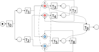
Using the above results, we can confirm the majority of TARs quickly, except for cases when TAR of a pair of consecutive transitions (t1t2t_{1}\bullet\cap\bullet t_{2}\neq\emptyset) cannot be confirmed using Thm. 4.2 and 4.3. In Fig. 6, we show such a special example, where additional checking using Algorithm 1 is necessary to confirm TAR.
Refer to caption
(a)
Refer to caption
(b)
Figure 6: A challenging cut-off event example that MEA rule does not cover

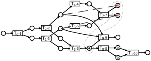
In Fig. 6, the TAR between the consecutive transitions T7subscript𝑇7T_{7} and T9subscript𝑇9T_{9} cannot be confirmed directly using MEA, because T7-7subscript𝑇7-7T_{7}\mbox{-}7 is a cut-off event. Neither can we discover this TAR by reusing the MEA related to T7-7subscript𝑇7-7T_{7}\mbox{-}7’s corresponding event T8-8subscript𝑇8-8T_{8}\mbox{-}8 based on Thm. 4.3, because Thm. 4.3 requires the corresponding places of the post conditions of the two events are identical, but in this case h(T7-7)h(T8-8)h(T_{7}\mbox{-}7\bullet)\neq h(T_{8}\mbox{-}8\bullet).

Therefore for such pairs of transitions, we are still faced by the challenge that MEA-based derivation rules cannot cover all TAR cases. For these cases, we need to utilize Algorithm 1 for general TAR checking.

What we have learned about MEA in the original TAR computation can also be easily extended to pTAR computation. By extending MEA to ‘neglect’ the silent events (events corresponding to silent transitions), we may identify pTAR from CFP using causal relations only.

Definition 4.3 (Silent Adjacency)

For two nodes n1,n2CEsubscript𝑛1subscript𝑛2𝐶𝐸n_{1},n_{2}\in C\cup E in an unfolding π=(O,h),O=(C,E,G)formulae-sequence𝜋𝑂𝑂𝐶𝐸𝐺\pi=(O,h),O=(C,E,G) such that n1<n2subscript𝑛1subscript𝑛2n_{1}<n_{2}, we say that n1subscript𝑛1n_{1} and n2subscript𝑛2n_{2} are in silent adjacency, denoted as n1sn2subscript𝑠subscript𝑛1subscript𝑛2n_{1}\triangleright_{s}n_{2} if and only if eE:n1<e<n2h(e):for-all𝑒𝐸subscript𝑛1𝑒subscript𝑛2𝑒\forall e\in E:n_{1}<e<n_{2}\Rightarrow h(e) is a silent transition.

Remark 4.1

It follows that n1sn2subscript𝑠subscript𝑛1subscript𝑛2n_{1}\triangleright_{s}n_{2} iff n1<n2subscript𝑛1subscript𝑛2n_{1}<n_{2} and npn2:n1<npn1snp\forall n_{p}\in\bullet n_{2}:n_{1}<n_{p}\Rightarrow n_{1}\triangleright_{s}n_{p}.

Theorem 4.4

For a pair of transitions t1,t2subscript𝑡1subscript𝑡2t_{1},t_{2} in a net system S𝑆S, t1<ptart2subscript𝑝𝑡𝑎𝑟subscript𝑡1subscript𝑡2t_{1}<_{ptar}t_{2} if and only if there exist in unfolding a pair of events e1,e2:h(e1)=t1,h(e2)=t2:subscript𝑒1subscript𝑒2formulae-sequencesubscript𝑒1subscript𝑡1subscript𝑒2subscript𝑡2e_{1},e_{2}:h(e_{1})=t_{1},h(e_{2})=t_{2} and e1se2subscript𝑠subscript𝑒1subscript𝑒2e_{1}\triangleright_{s}e_{2}.

Proof:

(\Rightarrow)For any given pair of transitions t1,t2subscript𝑡1subscript𝑡2t_{1},t_{2} in pTAR relation, according to Def. 2.6 there exists a marking Mssubscript𝑀𝑠M_{s} from which we can consecutively fire a sequence of transitions σ=t1,ti1,ti2,,tin,t2𝜎subscript𝑡1subscript𝑡subscript𝑖1subscript𝑡subscript𝑖2subscript𝑡subscript𝑖𝑛subscript𝑡2\sigma=\langle t_{1},t_{i_{1}},t_{i_{2}},...,t_{i_{n}},t_{2}\rangle, where ti1,ti2,,tinsubscript𝑡subscript𝑖1subscript𝑡subscript𝑖2subscript𝑡subscript𝑖𝑛t_{i_{1}},t_{i_{2}},...,t_{i_{n}} are silent tasks, i.e. Mst1M1ti1M2ti2subscript𝑡1subscript𝑀𝑠subscript𝑀1subscript𝑡subscript𝑖1subscript𝑀2subscript𝑡subscript𝑖2absentM_{s}\xrightarrow{t_{1}}M_{1}\xrightarrow{t_{i_{1}}}M_{2}\xrightarrow{t_{i_{2}}}tinMn+1t2Mn+2subscript𝑡subscript𝑖𝑛absentsubscript𝑀𝑛1subscript𝑡2subscript𝑀𝑛2\xrightarrow{t_{i_{n}}}M_{n+1}\xrightarrow{t_{2}}M_{n+2}. In the full unfolding Unf𝑈𝑛𝑓Unf of the net system S𝑆S, there is a configuration 𝒞𝒞\mathcal{C} in β𝛽\beta for which it holds that Cut(𝒞)=Ms𝐶𝑢𝑡𝒞subscript𝑀𝑠Cut(\mathcal{C})=M_{s}. Consequently, a sequence of events E=e1,ei1,ei2,,ein,e2𝐸subscript𝑒1subscript𝑒subscript𝑖1subscript𝑒subscript𝑖2subscript𝑒subscript𝑖𝑛subscript𝑒2E=\langle e_{1},e_{i_{1}},e_{i_{2}},...,e_{i_{n}},e_{2}\rangle: h(eik)=tik(1kn),h(e1)=t1,h(e2)=t2formulae-sequencesubscript𝑒subscript𝑖𝑘subscript𝑡subscript𝑖𝑘1𝑘𝑛formulae-sequencesubscript𝑒1subscript𝑡1subscript𝑒2subscript𝑡2h(e_{i_{k}})=t_{i_{k}}(1\leq k\leq n),h(e_{1})=t_{1},h(e_{2})=t_{2} can be added to 𝒞𝒞\mathcal{C}. For each event in {eik}subscript𝑒subscript𝑖𝑘\{e_{i_{k}}\} that occurs after e1subscript𝑒1e_{1}, because 𝒞E𝒞𝐸\mathcal{C}\cup E is a configuration, we have ¬(e1#eik)subscript𝑒1#subscript𝑒subscript𝑖𝑘\neg(e_{1}\#e_{i_{k}}), and therefore it holds either e1subscript𝑒1e_{1} co𝑐𝑜co eiksubscript𝑒subscript𝑖𝑘e_{i_{k}} or e1<eiksubscript𝑒1subscript𝑒subscript𝑖𝑘e_{1}<e_{i_{k}} (eik<e1subscript𝑒subscript𝑖𝑘subscript𝑒1e_{i_{k}}<e_{1} does not hold because e1subscript𝑒1e_{1} can be added before eiksubscript𝑒subscript𝑖𝑘e_{i_{k}}). Similarly, we know that e1<e2subscript𝑒1subscript𝑒2e_{1}<e_{2}, because e1subscript𝑒1e_{1} co e2subscript𝑒2e_{2} must not hold (otherwise, we would have t1<tart2subscript𝑡𝑎𝑟subscript𝑡1subscript𝑡2t_{1}<_{tar}t_{2}, which contradicts with t1<ptart2subscript𝑝𝑡𝑎𝑟subscript𝑡1subscript𝑡2t_{1}<_{ptar}t_{2}). Consider any event e:e1<e<e2:𝑒subscript𝑒1𝑒subscript𝑒2e:e_{1}<e<e_{2}. Since e1<esubscript𝑒1𝑒e_{1}<e, we know that e𝒞𝑒𝒞e\not\in\mathcal{C}, and consequently eE𝑒𝐸e\in E. Therefore, e𝑒e must belong to {eik}subscript𝑒subscript𝑖𝑘\{e_{i_{k}}\}, and h(e)𝑒h(e) is a silent transition. By Def. 4.3, we have e1se2subscript𝑠subscript𝑒1subscript𝑒2e_{1}\triangleright_{s}e_{2}.

(\Leftarrow) Let E1={eik[e2]|e1eik<e2}subscript𝐸1conditional-setsubscript𝑒subscript𝑖𝑘delimited-[]subscript𝑒2subscript𝑒1subscript𝑒subscript𝑖𝑘subscript𝑒2E_{1}=\{e_{i_{k}}\in[e_{2}]|e_{1}\leq e_{i_{k}}<e_{2}\}={ei1,ei2,,ein,n=|E1|}subscript𝑒subscript𝑖1subscript𝑒subscript𝑖2subscript𝑒subscript𝑖𝑛𝑛subscript𝐸1\{e_{i_{1}},e_{i_{2}},...,e_{i_{n}},n=|E_{1}|\}, where eip<eiqp<qsubscript𝑒subscript𝑖𝑝subscript𝑒subscript𝑖𝑞𝑝𝑞e_{i_{p}}<e_{i_{q}}\Rightarrow p<q. As e1se2subscript𝑠subscript𝑒1subscript𝑒2e_{1}\triangleright_{s}e_{2} it holds that ei1=e1subscript𝑒subscript𝑖1subscript𝑒1e_{i_{1}}=e_{1} and {h(ei2),h(ei3),,h(ein)}subscript𝑒subscript𝑖2subscript𝑒subscript𝑖3subscript𝑒subscript𝑖𝑛\{h(e_{i_{2}}),h(e_{i_{3}}),...,h(e_{i_{n}})\} are all silent transitions. By Lemma 4.1 and Lemma 4.3, [e2]\{e2}\delimited-[]subscript𝑒2subscript𝑒2[e_{2}]\backslash\{e_{2}\} is a configuration, and h(e2)subscript𝑒2h(e_{2}) is enabled at Mn+1=Mark([e2]\{e2})subscript𝑀𝑛1𝑀𝑎𝑟𝑘\delimited-[]subscript𝑒2subscript𝑒2M_{n+1}=Mark([e_{2}]\backslash\{e_{2}\}).

Consider einsubscript𝑒subscript𝑖𝑛e_{i_{n}}. It holds that e[e2]\{e2},eineformulae-sequencefor-all𝑒\delimited-[]subscript𝑒2subscript𝑒2not-less-thansubscript𝑒subscript𝑖𝑛𝑒\forall e\in[e_{2}]\backslash\{e_{2}\},e_{i_{n}}\not<e, otherwise it contradicts with eip<eiqp<qsubscript𝑒subscript𝑖𝑝subscript𝑒subscript𝑖𝑞𝑝𝑞e_{i_{p}}<e_{i_{q}}\Rightarrow p<q. Therefore einMax([e2]\{e2})subscript𝑒subscript𝑖𝑛𝑀𝑎𝑥\delimited-[]subscript𝑒2subscript𝑒2e_{i_{n}}\in Max([e_{2}]\backslash\{e_{2}\}). Again, by Lemma 4.1 and Lemma 4.3, [e2]\{e2,ein}\delimited-[]subscript𝑒2subscript𝑒2subscript𝑒subscript𝑖𝑛[e_{2}]\backslash\{e_{2},e_{i_{n}}\} is a configuration, and h(ein)subscript𝑒subscript𝑖𝑛h(e_{i_{n}}) is enabled at Mn=Mark([e2]\{e2,ein}M_{n}=Mark([e_{2}]\backslash\{e_{2},e_{i_{n}}\} and Mnh(ein)Mn+1subscript𝑒subscript𝑖𝑛subscript𝑀𝑛subscript𝑀𝑛1M_{n}\xrightarrow{h(e_{i_{n}})}M_{n+1}. By recursively applying the above process, we have eikMax([e2]\{e2,ein,,eik+1})(k1)subscript𝑒subscript𝑖𝑘𝑀𝑎𝑥\delimited-[]subscript𝑒2subscript𝑒2subscript𝑒subscript𝑖𝑛subscript𝑒subscript𝑖𝑘1𝑘1e_{i_{k}}\in Max([e_{2}]\backslash\{e_{2},e_{i_{n}},...,e_{i_{k+1}}\})(k\geq 1). In other words, from M1=Mark[e1]subscript𝑀1𝑀𝑎𝑟𝑘delimited-[]subscript𝑒1M_{1}=Mark[e_{1}], there exists a firing sequence M1h(ei1)M2h(ei2)h(ein)Mn+1subscript𝑒subscript𝑖1subscript𝑀1subscript𝑀2subscript𝑒subscript𝑖2subscript𝑒subscript𝑖𝑛subscript𝑀𝑛1M_{1}\xrightarrow{h(e_{i_{1}})}M_{2}\xrightarrow{h(e_{i_{2}})}...\xrightarrow{h(e_{i_{n}})}M_{n+1}, and h(e2)subscript𝑒2h(e_{2}) is enabled at Mn+1subscript𝑀𝑛1M_{n+1}. As ei1=e1subscript𝑒subscript𝑖1subscript𝑒1e_{i_{1}}=e_{1} and {h(ei2),h(ei3),,h(ein)}subscript𝑒subscript𝑖2subscript𝑒subscript𝑖3subscript𝑒subscript𝑖𝑛\{h(e_{i_{2}}),h(e_{i_{3}}),...,h(e_{i_{n}})\} are all silent transitions, we have h(e1)=t1<ptart2=h(e2)subscript𝑒1subscript𝑡1subscript𝑝𝑡𝑎𝑟subscript𝑡2subscript𝑒2h(e_{1})=t_{1}<_{ptar}t_{2}=h(e_{2}). ∎

In order to recover the truncated silent adjacency structures, we propose to extend the original CFP after cut-off events, until at least one silent adjacency structure can be identified for each pair of transitions in pTAR.
Refer to caption
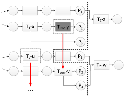
Figure 7: The handling of cut-off event ‘chains’ is a major challenge

However, because the events in silent adjacency structures may be truncated by cut-off events, the silent adjacency structures may not be completely available in CFP. Fig. 7 shows a possible CFP, where a cut-off event TINV-ysubscript𝑇𝐼𝑁𝑉-𝑦T_{INV}\mbox{-}y is formed by a silent transition in a loop structure. It causes the ssubscript𝑠\triangleright_{s} structure between T1-xsubscript𝑇1-𝑥T_{1}\mbox{-}x and T2-zsubscript𝑇2-𝑧T_{2}\mbox{-}z to be truncated.

The idea of looking behind the corresponding events does not work here, because it is not guaranteed that there is an isomorphic silent adjacency structure after Tcorr-vsubscript𝑇𝑐𝑜𝑟𝑟-𝑣T_{corr}\mbox{-}v. For example, there might be other cut-off events (in this example, it is Tc-usubscript𝑇𝑐-𝑢T_{c}\mbox{-}u) that are in co𝑐𝑜co with Tcorr-vsubscript𝑇𝑐𝑜𝑟𝑟-𝑣T_{corr}\mbox{-}v and are precedent to the silent adjacency structure after Tcorr-vsubscript𝑇𝑐𝑜𝑟𝑟-𝑣T_{corr}\mbox{-}v. In this case, Tc-usubscript𝑇𝑐-𝑢T_{c}\mbox{-}u truncates T2-wsubscript𝑇2-𝑤T_{2}\mbox{-}w after Tcorr-vsubscript𝑇𝑐𝑜𝑟𝑟-𝑣T_{corr}\mbox{-}v, so now we are forced to seek an isomorphic silent adjacency structure after Tc-usubscript𝑇𝑐-𝑢T_{c}\mbox{-}u’s corresponding event that may confirm T1<ptarT2subscript𝑝𝑡𝑎𝑟subscript𝑇1subscript𝑇2T_{1}<_{ptar}T_{2}. If such patterns keep repeating, it will make efficient computation impossible. One direct solution is to use coverability checking as in Algorithm 1 to deal with cases involving cut-off events, as Algorithm 1 does.

Algorithm 1 Accelerated TAR Derivation (IMPROVED)
1:function IMPROVED(S,π𝑆𝜋S,\pi)
2:     TAR𝑇𝐴𝑅TAR\leftarrow\emptyset
3:     for each e1πsubscript𝑒1𝜋e_{1}\in\pi do
4:     for each e2:(e1e2)(e1e_{2}:(e_{1}\triangleright e_{2})\vee(e_{1} co e2)(e1se2)e_{2})\vee(e_{1}\triangleright_{s}e_{2}) do
5:     TARTAR{h(e1),h(e2)}𝑇𝐴𝑅𝑇𝐴𝑅subscript𝑒1subscript𝑒2TAR\leftarrow TAR\cup\{\langle h(e_{1}),h(e_{2})\rangle\}
6:     for each cut-off event e𝑒e and its corr. event esuperscript𝑒e^{\prime} do
7:     if h(e)=h(eh(e\bullet)=h(e^{\prime}\bullet) then
8:     for each e2:ee2:subscript𝑒2superscript𝑒subscript𝑒2e_{2}:e^{\prime}\triangleright e_{2} do TARTAR{h(e),h(e2)}𝑇𝐴𝑅𝑇𝐴𝑅𝑒subscript𝑒2TAR\leftarrow TAR\cup\{\langle h(e),h(e_{2})\rangle\}
9:     for each t1,t2Ssubscript𝑡1subscript𝑡2𝑆t_{1},t_{2}\in S do
10:     /*we can further restrict to t1,t2:t1t2t_{1},t_{2}:t_{1}\bullet\cap\bullet t_{2}\neq\emptyset if we do not compute pTAR*/
11:     if h(e1),h(e2)TARsubscript𝑒1subscript𝑒2𝑇𝐴𝑅\langle h(e_{1}),h(e_{2})\rangle\not\in TAR then
12:     Reduce t1<tart2subscript𝑡𝑎𝑟subscript𝑡1subscript𝑡2t_{1}<_{tar}t_{2} or t1<ptart2subscript𝑝𝑡𝑎𝑟subscript𝑡1subscript𝑡2t_{1}<_{ptar}t_{2} to a marking M𝑀M’s coverability
13:     if M𝑀M is coverable then TARTAR{t1,t2}𝑇𝐴𝑅𝑇𝐴𝑅subscript𝑡1subscript𝑡2TAR\leftarrow TAR\cup\{\langle t_{1},t_{2}\rangle\}
14:     return TAR𝑇𝐴𝑅TAR
15:end function

From Line 3similar-to\sim8), Algorithm 1 attempts to early-confirm TAR/pTAR using the accelerative rules. After that, coverability based approach is applied only to those transition pairs that have not been early-confirmed.

5 Computing TAR/pTAR with Continued Unfolding

Apart from coverability checking, another strategy could be extending the CFP structure after cut-off events. Through the following analysis, we show how to extend just enough transitions for pTAR computation and avoid unnecessary extensions.

5.1 Continued Unfolding After Cut-off Events

Definition 5.1 (Local Silent Extension)

Let β𝛽\beta be the full unfolding of a net system S𝑆S. The local silent extensions of β𝛽\beta with respect to an event e1subscript𝑒1e_{1}, denoted as LSE(β,e1)𝐿𝑆𝐸𝛽subscript𝑒1LSE(\beta,e_{1}), is defined as a set of events {e=(t,B)}𝑒𝑡𝐵\{e=(t,B)\}, in which for each event e=(t,B)𝑒𝑡𝐵e=(t,B), B𝐵B is a co-set of conditions in β𝛽\beta and t𝑡t is a transitions of S𝑆S, h(B)=th(B)=\bullet t such that

  • (1)

    cB:(e1sc)(e1\forall c\in B:(e_{1}\triangleright_{s}c)\vee(e_{1} co c𝑐c), and cB:e1sc:𝑐𝐵subscript𝑠subscript𝑒1𝑐\exists c\in B:e_{1}\triangleright_{s}c

  • (2)

    β𝛽\beta contains no event e𝑒e satisfying h(e)=t𝑒𝑡h(e)=t and e=B\bullet e=B

Intuitively, LSE(β,e1)𝐿𝑆𝐸𝛽subscript𝑒1LSE(\beta,e_{1}) extends the original branching process β𝛽\beta by only adding any event that is in silent adjacency relation with e1subscript𝑒1e_{1}. By recursively doing this, we get an extended CFP in which we shall find all the silent adjacency structures we need, that is:

Definition 5.2 (Silently Continued Branching Process)

Let π𝜋\pi be the CFP of a net system S𝑆S and e1subscript𝑒1e_{1} an event in π𝜋\pi. The silently continued branching processes after e1subscript𝑒1e_{1}, denoted as β(e1)𝛽subscript𝑒1\beta\in\mathcal{L}(e_{1}) are a set of branching processes of S𝑆S such that:

  • -

    π(e)𝜋𝑒\pi\in\mathcal{L}(e)

  • -

    β:β(e1):for-allsuperscript𝛽superscript𝛽subscript𝑒1\forall\beta^{\prime}:\beta^{\prime}\in\mathcal{L}(e_{1}) and e=(t,B)LSE(β,e1)𝑒𝑡𝐵𝐿𝑆𝐸superscript𝛽subscript𝑒1e=(t,B)\in LSE(\beta^{\prime},e_{1}), β=β{e}e(e)\beta=\beta^{\prime}\cup\{e\}\cup e\bullet\in\mathcal{L}(e) .

Intuitively, silently continued branching processes are derived by recursively extending the original CFP behind e1subscript𝑒1e_{1} using LSE𝐿𝑆𝐸LSE. We call the maximal silently continued branching process w.r.t. a cut-off event e1subscript𝑒1e_{1} in CFP its silently continued unfolding, denoted as βe1subscript𝛽subscript𝑒1\beta_{e_{1}}, which can be constructed with Algorithm 1.

Algorithm 1 Deriving silently continued unfolding after e1subscript𝑒1e_{1}
1:function silently-continued-unfolding(S,π,e1𝑆𝜋subscript𝑒1S,\pi,e_{1})
2:     βe1πsubscript𝛽subscript𝑒1𝜋\beta_{e_{1}}\leftarrow\pi
3:     lseLSE(βe1,e1)𝑙𝑠𝑒𝐿𝑆𝐸subscript𝛽subscript𝑒1subscript𝑒1lse\leftarrow LSE(\beta_{e_{1}},e_{1})
4:     while lse𝑙𝑠𝑒lse\neq\emptyset do
5:     take an event e=(t,B)𝑒𝑡𝐵e=(t,B) out of lse𝑙𝑠𝑒lse and add it to βe1subscript𝛽subscript𝑒1\beta_{e_{1}} with a condition (c,e)𝑐𝑒(c,e) for every output place p𝑝p of t𝑡t.
6:     lseLSE(βe1,e1)𝑙𝑠𝑒𝐿𝑆𝐸subscript𝛽subscript𝑒1subscript𝑒1lse\leftarrow LSE(\beta_{e_{1}},e_{1})
7:     endwhile
8:end function

Similar to the original unfolding algorithm [17], Algorithm 1 does not necessarily terminate. This suggest we need to introduce a new kind of termination condition for silently continued branching processes (i.e. a new kind of cut-off event ). But let us come back to this later. Now, with the denotation of βe1subscript𝛽subscript𝑒1\beta_{e_{1}} and Algorithm 1, we can prove that for each pair of transitions in pTAR, at least one silent adjacency structure could be found in βe1subscript𝛽subscript𝑒1\beta_{e_{1}}.

Theorem 5.1

Let β𝛽\beta and π𝜋\pi be the full unfolding and CFP of a net system S𝑆S respectively. For every pair e1,e2:e1e2:subscript𝑒1subscript𝑒2subscript𝑒1subscript𝑒2e_{1},e_{2}:e_{1}\triangleright e_{2} in β𝛽\beta, there exists an event e1:h(e1)=h(e1):superscriptsubscript𝑒1superscriptsubscript𝑒1subscript𝑒1e_{1}^{\prime}:h(e_{1}^{\prime})=h(e_{1}) in π𝜋\pi, such that in βe1subscript𝛽subscript𝑒1\beta_{e_{1}}, there is an event e2:h(e2)=h(e2):superscriptsubscript𝑒2superscriptsubscript𝑒2subscript𝑒2e_{2}^{\prime}:h(e_{2}^{\prime})=h(e_{2}) and e1e2superscriptsubscript𝑒1superscriptsubscript𝑒2e_{1}^{\prime}\triangleright e_{2}^{\prime}.

Proof:

Let E={eik:e1<eik<e2}𝐸conditional-setsubscript𝑒subscript𝑖𝑘subscript𝑒1subscript𝑒subscript𝑖𝑘subscript𝑒2E=\{e_{i_{k}}:e_{1}<e_{i_{k}}<e_{2}\}, 1kn1𝑘𝑛1\leq k\leq n and restrict, without loss of generality, that eip<eiqp<qsubscript𝑒subscript𝑖𝑝subscript𝑒subscript𝑖𝑞𝑝𝑞e_{i_{p}}<e_{i_{q}}\Rightarrow p<q. Since [e2]delimited-[]subscript𝑒2[e_{2}] is a configuration, by recursively applying Lemma 4.1, we know that

𝒞=[e2]\{e2}\{eik}\{eik1}\\{ei1}\{e1}𝒞\delimited-[]subscript𝑒2subscript𝑒2subscript𝑒subscript𝑖𝑘subscript𝑒subscript𝑖𝑘1subscript𝑒subscript𝑖1subscript𝑒1\mathcal{C}=[e_{2}]\backslash\{e_{2}\}\backslash\{e_{i_{k}}\}\backslash\{e_{i_{k-1}}\}\backslash...\backslash\{e_{i_{1}}\}\backslash\{e_{1}\}

is a configuration. Consequently, it is easy to prove that 𝒞{e1}direct-sum𝒞subscript𝑒1\mathcal{C}\oplus\{e_{1}\},𝒞{e1,ei1}direct-sum𝒞subscript𝑒1subscript𝑒subscript𝑖1\mathcal{C}\oplus\{e_{1},e_{i_{1}}\},…,𝒞{e1,ei1,,ein}direct-sum𝒞subscript𝑒1subscript𝑒subscript𝑖1subscript𝑒subscript𝑖𝑛\mathcal{C}\oplus\{e_{1},e_{i_{1}},...,e_{i_{n}}\} and 𝒞{e1,ei1,,ein,e2}=[e2]direct-sum𝒞subscript𝑒1subscript𝑒subscript𝑖1subscript𝑒subscript𝑖𝑛subscript𝑒2delimited-[]subscript𝑒2\mathcal{C}\oplus\{e_{1},e_{i_{1}},...,e_{i_{n}},e_{2}\}=[e_{2}] are all configurations.

By Property 4.1, we know that in π𝜋\pi there exists a configuration 𝒞superscript𝒞\mathcal{C^{\prime}} such that Mark(𝒞)=Mark(𝒞)𝑀𝑎𝑟𝑘superscript𝒞𝑀𝑎𝑟𝑘𝒞Mark(\mathcal{C^{\prime}})=Mark(\mathcal{C}) and 𝒞superscript𝒞\mathcal{C^{\prime}} does not contain any cut-off events.

As Mark(𝒞)=Mark(𝒞)𝑀𝑎𝑟𝑘superscript𝒞𝑀𝑎𝑟𝑘𝒞Mark(\mathcal{C^{\prime}})=Mark(\mathcal{C}), 𝒞absentsuperscript𝒞\Uparrow\mathcal{C^{\prime}} is isomorphic with 𝒞absent𝒞\Uparrow\mathcal{C}. Let I12superscriptsubscript𝐼12I_{1}^{2} be the isomorphism between 𝒞𝒞\mathcal{C} and 𝒞superscript𝒞\mathcal{C^{\prime}}. Let e1=I12(e1)subscriptsuperscript𝑒1superscriptsubscript𝐼12subscript𝑒1e^{\prime}_{1}=I_{1}^{2}(e_{1}). Since 𝒞{e1}direct-sum𝒞subscript𝑒1\mathcal{C}\oplus\{e_{1}\} is a configuration, 𝒞{e1}direct-sumsuperscript𝒞subscriptsuperscript𝑒1\mathcal{C^{\prime}}\oplus\{e^{\prime}_{1}\} is also a configuration. And as 𝒞superscript𝒞\mathcal{C^{\prime}} does not contain any cut-off event, 𝒞{e1}superscript𝒞superscriptsubscript𝑒1\mathcal{C^{\prime}}\cup\{e_{1}^{\prime}\} is contained in π𝜋\pi.

Let eik=I12(ik)subscriptsuperscript𝑒subscript𝑖𝑘superscriptsubscript𝐼12subscript𝑖𝑘e^{\prime}_{i_{k}}=I_{1}^{2}(i_{k}) (1kn)1𝑘𝑛(1\leq k\leq n), and e2=I12(e2)subscriptsuperscript𝑒2superscriptsubscript𝐼12subscript𝑒2e^{\prime}_{2}=I_{1}^{2}(e_{2}). Since 𝒞{e1,ei1,,eik,e2}direct-sum𝒞subscript𝑒1subscript𝑒subscript𝑖1subscript𝑒subscript𝑖𝑘subscript𝑒2\mathcal{C}\oplus\{e_{1},e_{i_{1}},...,e_{i_{k}},e_{2}\} is a configuration, 𝒞{e1,ei1,,eik,e2}direct-sumsuperscript𝒞subscriptsuperscript𝑒1subscriptsuperscript𝑒subscript𝑖1subscriptsuperscript𝑒subscript𝑖𝑘subscriptsuperscript𝑒2\mathcal{C^{\prime}}\oplus\{e^{\prime}_{1},e^{\prime}_{i_{1}},...,e^{\prime}_{i_{k}},e^{\prime}_{2}\} should also be a configuration in β𝛽\beta (but not necessarily fully contained in π𝜋\pi). For Algorithm 1 , we now prove that 𝒞{e1,ei1,,ein,e2}direct-sumsuperscript𝒞subscriptsuperscript𝑒1subscriptsuperscript𝑒subscript𝑖1subscriptsuperscript𝑒subscript𝑖𝑛subscriptsuperscript𝑒2\mathcal{C^{\prime}}\oplus\{e^{\prime}_{1},e^{\prime}_{i_{1}},...,e^{\prime}_{i_{n}},e^{\prime}_{2}\} are in βe1subscript𝛽subscriptsuperscript𝑒1\beta_{e^{\prime}_{1}}. First, because 𝒞{e1}πβe1superscript𝒞subscriptsuperscript𝑒1𝜋subscript𝛽subscriptsuperscript𝑒1\mathcal{C^{\prime}}\cup\{e^{\prime}_{1}\}\subseteq\pi\subseteq\beta_{e^{\prime}_{1}}, e1subscriptsuperscript𝑒1e^{\prime}_{1} is contained in βe1subscript𝛽subscriptsuperscript𝑒1\beta_{e^{\prime}_{1}}. For events in {eik}subscriptsuperscript𝑒subscript𝑖𝑘\{e^{\prime}_{i_{k}}\}, we prove by induction:

(a) When k=1𝑘1k=1, because (𝒞{e1}){ei1}direct-sum𝒞subscript𝑒1subscript𝑒subscript𝑖1(\mathcal{C}\cup\{e_{1}\})\oplus\{e_{i_{1}}\} is a configuration, (𝒞{e1}){ei1}direct-sum𝒞subscriptsuperscript𝑒1subscriptsuperscript𝑒subscript𝑖1(\mathcal{C}\cup\{e^{\prime}_{1}\})\oplus\{e^{\prime}_{i_{1}}\} is also a configuration. By isomorphism, as e1<ei1subscript𝑒1subscript𝑒subscript𝑖1e_{1}<e_{i_{1}}, it holds that e1<ei1subscriptsuperscript𝑒1subscriptsuperscript𝑒subscript𝑖1e^{\prime}_{1}<e^{\prime}_{i_{1}}. Therefore B=ei1Cut(𝒞{e1})βe1B=\bullet e^{\prime}_{i_{1}}\subseteq Cut(\mathcal{C^{\prime}}\oplus\{e^{\prime}_{1}\})\subseteq\beta_{e^{\prime}_{1}} and cB:e1<c:𝑐𝐵subscript𝑒1𝑐\exists c\in B:e_{1}<c (condition (1) of Def. 4.3). For any c𝑐c in B𝐵B, we have {e|e1<e<c}=conditional-set𝑒subscriptsuperscript𝑒1𝑒𝑐\{e|e^{\prime}_{1}<e<c\}=\emptyset, so condition (2) of Def. 4.3 holds trivially. Therefore, at Line 3 of Algorithm 1, if βe1subscript𝛽subscriptsuperscript𝑒1\beta_{e^{\prime}_{1}} does not already contain ei1=(h(ei1),B)subscriptsuperscript𝑒subscript𝑖1subscriptsuperscript𝑒subscript𝑖1𝐵e^{\prime}_{i_{1}}=(h(e^{\prime}_{i_{1}}),B), then condition (3) is satisfied as well, and ei1subscriptsuperscript𝑒subscript𝑖1e^{\prime}_{i_{1}} will be added to lse𝑙𝑠𝑒lse and eventually inserted into βe1subscript𝛽subscriptsuperscript𝑒1\beta_{e^{\prime}_{1}} at Line 5.

(b) For any k>1𝑘1k>1, assume that 𝒞{e1,ei1,,eik1}direct-sumsuperscript𝒞subscriptsuperscript𝑒1subscriptsuperscript𝑒subscript𝑖1subscriptsuperscript𝑒subscript𝑖𝑘1\mathcal{C^{\prime}}\oplus\{e^{\prime}_{1},e^{\prime}_{i_{1}},...,e^{\prime}_{i_{k}-1}\} can eventually be contained in βe1subscript𝛽subscriptsuperscript𝑒1\beta_{e^{\prime}_{1}}. If eiksubscriptsuperscript𝑒subscript𝑖𝑘e^{\prime}_{i_{k}} is in π𝜋\pi, then the induction hypothesis holds trivially. Next we consider the case of eiksubscriptsuperscript𝑒subscript𝑖𝑘e^{\prime}_{i_{k}} not being π𝜋\pi.

Let B=eikB=\bullet e_{i_{k}}. By isomorphism, 𝒞{e1,ei1,,eik1}{eik}direct-sumsuperscript𝒞subscriptsuperscript𝑒1subscriptsuperscript𝑒subscript𝑖1subscriptsuperscript𝑒subscript𝑖𝑘1subscriptsuperscript𝑒subscript𝑖𝑘\mathcal{C^{\prime}}\oplus\{e^{\prime}_{1},e^{\prime}_{i_{1}},...,e^{\prime}_{i_{k}-1}\}\oplus\{e^{\prime}_{i_{k}}\} is also a configuration, so we have BCut(𝒞{e1,ei1,,eik1})𝐵𝐶𝑢𝑡direct-sumsuperscript𝒞subscriptsuperscript𝑒1subscriptsuperscript𝑒subscript𝑖1subscriptsuperscript𝑒subscript𝑖𝑘1B\subseteq Cut(\mathcal{C^{\prime}}\oplus\{e^{\prime}_{1},e^{\prime}_{i_{1}},...,e^{\prime}_{i_{k}-1}\}). As e1<eiksubscript𝑒1subscript𝑒subscript𝑖𝑘e_{1}<e_{i_{k}}, it holds that e1<eiksubscriptsuperscript𝑒1subscriptsuperscript𝑒subscript𝑖𝑘e^{\prime}_{1}<e^{\prime}_{i_{k}} and consequently cB:e1<c:𝑐𝐵subscriptsuperscript𝑒1𝑐\exists c\in B:e^{\prime}_{1}<c. Therefore condition (1) of Def. 4.3 holds.

Consider EM={e|e1<e<c,cB}subscript𝐸𝑀conditional-set𝑒formulae-sequencesubscriptsuperscript𝑒1𝑒𝑐𝑐𝐵E_{M}=\{e|e^{\prime}_{1}<e<c,c\in B\}. If EM=subscript𝐸𝑀E_{M}=\emptyset, then in the same manner of (a) we can conclude that both condition (1), (2) and (3) of Def. 4.3 will be satisfied at Line 3 of Algorithm 1, and eiksubscriptsuperscript𝑒subscript𝑖𝑘e^{\prime}_{i_{k}} will be added in βe1subscript𝛽subscriptsuperscript𝑒1\beta_{e^{\prime}_{1}} if it is not already in π𝜋\pi.Otherwise, if EM={e|e1<e<c,cB}subscript𝐸𝑀conditional-set𝑒formulae-sequencesubscriptsuperscript𝑒1𝑒𝑐𝑐𝐵E_{M}=\{e|e^{\prime}_{1}<e<c,c\in B\} is not empty, then it must hold that EM{ei1,,eik1}subscript𝐸𝑀subscriptsuperscript𝑒subscript𝑖1subscriptsuperscript𝑒subscript𝑖𝑘1E_{M}\subseteq\{e^{\prime}_{i_{1}},...,e^{\prime}_{i_{k}-1}\}. (This is because cCut(𝒞{e1,ei1,,eik1})𝑐𝐶𝑢𝑡direct-sumsuperscript𝒞subscriptsuperscript𝑒1subscriptsuperscript𝑒subscript𝑖1subscriptsuperscript𝑒subscript𝑖𝑘1c\in Cut(\mathcal{C^{\prime}}\oplus\{e^{\prime}_{1},e^{\prime}_{i_{1}},...,e^{\prime}_{i_{k}-1}\}), and in 𝒞{e1,ei1,,eik1}direct-sumsuperscript𝒞subscriptsuperscript𝑒1subscriptsuperscript𝑒subscript𝑖1subscriptsuperscript𝑒subscript𝑖𝑘1\mathcal{C^{\prime}}\oplus\{e^{\prime}_{1},e^{\prime}_{i_{1}},...,e^{\prime}_{i_{k}-1}\}, {ei1,,eik1}subscriptsuperscript𝑒subscript𝑖1subscriptsuperscript𝑒subscript𝑖𝑘1\{e^{\prime}_{i_{1}},...,e^{\prime}_{i_{k}-1}\} are the only events added after 𝒞{e1}direct-sum𝒞subscriptsuperscript𝑒1\mathcal{C}\oplus\{e^{\prime}_{1}\}.) As {h(ei1),,h(eik1)}subscriptsuperscript𝑒subscript𝑖1subscriptsuperscript𝑒subscript𝑖𝑘1\{h(e^{\prime}_{i_{1}}),...,h(e^{\prime}_{i_{k}-1})\} are all silent transitions, condition (2) for LSE𝐿𝑆𝐸LSE also holds.

If 𝒞{e1,ei1,,eik1}direct-sumsuperscript𝒞subscriptsuperscript𝑒1subscriptsuperscript𝑒subscript𝑖1subscriptsuperscript𝑒subscript𝑖𝑘1\mathcal{C^{\prime}}\oplus\{e^{\prime}_{1},e^{\prime}_{i_{1}},...,e^{\prime}_{i_{k}-1}\} are already contained in π𝜋\pi in the beginning, then eiksubscriptsuperscript𝑒subscript𝑖𝑘e^{\prime}_{i_{k}} can be added to lse𝑙𝑠𝑒lse at Line 3 and eventually into βe1subscript𝛽subscriptsuperscript𝑒1\beta_{e^{\prime}_{1}} at Line 5. Otherwise, by our induction hypothesis, the events in {ei1,,eik1}subscriptsuperscript𝑒subscript𝑖1subscriptsuperscript𝑒subscript𝑖𝑘1\{e^{\prime}_{i_{1}},...,e^{\prime}_{i_{k}-1}\} which are not in π𝜋\pi will be added into βe1subscript𝛽subscriptsuperscript𝑒1\beta_{e^{\prime}_{1}} by Line 5. Immediately after the last one of such events are added into βe1subscript𝛽subscriptsuperscript𝑒1\beta_{e^{\prime}_{1}} at Line 5, condition (3) for LSE𝐿𝑆𝐸LSE is satisfied, and eiksubscriptsuperscript𝑒subscript𝑖𝑘e^{\prime}_{i_{k}} will be added to lse𝑙𝑠𝑒lse and eventually into βe1subscript𝛽subscriptsuperscript𝑒1\beta_{e^{\prime}_{1}} at Line 5.

By (a) and (b), by induction we know that 𝒞{e1,ei1,,eik}direct-sumsuperscript𝒞subscriptsuperscript𝑒1subscriptsuperscript𝑒subscript𝑖1subscriptsuperscript𝑒subscript𝑖𝑘\mathcal{C^{\prime}}\oplus\{e^{\prime}_{1},e^{\prime}_{i_{1}},...,e^{\prime}_{i_{k}}\} is either contained in π𝜋\pi, or can be added to βe1subscript𝛽subscriptsuperscript𝑒1\beta_{e^{\prime}_{1}} in the loop of Line 4-8.

As we have previously shown, 𝒞{e1,ei1,,eik}{e2}direct-sumsuperscript𝒞subscriptsuperscript𝑒1subscriptsuperscript𝑒subscript𝑖1subscriptsuperscript𝑒subscript𝑖𝑘subscriptsuperscript𝑒2\mathcal{C^{\prime}}\oplus\{e^{\prime}_{1},e^{\prime}_{i_{1}},...,e^{\prime}_{i_{k}}\}\oplus\{e^{\prime}_{2}\} is also a configuration. By the similar reasoning in (b), we know that 𝒞{e1,ei1,,eik}{e2}direct-sumsuperscript𝒞subscriptsuperscript𝑒1subscriptsuperscript𝑒subscript𝑖1subscriptsuperscript𝑒subscript𝑖𝑘subscriptsuperscript𝑒2\mathcal{C^{\prime}}\oplus\{e^{\prime}_{1},e^{\prime}_{i_{1}},...,e^{\prime}_{i_{k}}\}\oplus\{e^{\prime}_{2}\} will eventually be contained in βe1subscript𝛽superscriptsubscript𝑒1\beta_{e_{1}^{\prime}}, and that e1<e2,{e|e1<e<e2}{ei1,,eik}formulae-sequencesubscriptsuperscript𝑒1subscriptsuperscript𝑒2conditional-set𝑒subscriptsuperscript𝑒1𝑒subscriptsuperscript𝑒2subscriptsuperscript𝑒subscript𝑖1subscriptsuperscript𝑒subscript𝑖𝑘e^{\prime}_{1}<e^{\prime}_{2},\{e|e^{\prime}_{1}<e<e^{\prime}_{2}\}\subseteq\{e^{\prime}_{i_{1}},...,e^{\prime}_{i_{k}}\}. As {h(ei1),,h(eik)}subscriptsuperscript𝑒subscript𝑖1subscriptsuperscript𝑒subscript𝑖𝑘\{h(e^{\prime}_{i_{1}}),...,h(e^{\prime}_{i_{k}})\} are all silent transitions, we have e1se2subscript𝑠subscriptsuperscript𝑒1subscriptsuperscript𝑒2e^{\prime}_{1}\triangleright_{s}e^{\prime}_{2}. ∎

5.2 Determine When to Stop a Silently Continued Unfolding

Being similar with Esparza’s original unfolding algorithm [17], Algorithm 1 does not necessarily terminate. To avoid state-explosion and infinite unfolding, we should stop silently continued unfolding when enough information has been unfolded for complete pTAR computation. In order to do this, we introduce a new type of cut-off events in silently continued unfolding as follows:

Definition 5.3

(Local Cut-off Events in Silently Continued Unfolding) Given two events ea,ebsubscript𝑒𝑎subscript𝑒𝑏e_{a},e_{b} in βe1\π\subscript𝛽subscript𝑒1𝜋\beta_{e_{1}}\backslash\pi, let Ea={e[ea]:eπ}subscript𝐸𝑎conditional-set𝑒delimited-[]subscript𝑒𝑎𝑒𝜋E_{a}=\{e\in[e_{a}]:e\not\in\pi\}, Eb={e[eb]:eπ}subscript𝐸𝑏conditional-set𝑒delimited-[]subscript𝑒𝑏𝑒𝜋E_{b}=\{e\in[e_{b}]:e\not\in\pi\}. We say that ebsubscript𝑒𝑏e_{b} is in the set of local cut-off events in silently continued unfolding βe1\π\subscript𝛽subscript𝑒1𝜋\beta_{e_{1}}\backslash\pi, denoted as cut-offe1subscript𝑒1{}_{e_{1}}, if

  • (1)

    Min(Ea)Min(Eb)Min(\bullet E_{a})\subseteq Min(\bullet E_{b}),

  • (2)

    h((Ea\Ea)(Min(Eb)\Min(Ea)))=h(Eb\Eb)h((E_{a}\bullet\backslash\bullet E_{a})\cup(Min(\bullet E_{b})\backslash Min(\bullet E_{a})))=h(E_{b}\bullet\backslash\bullet E_{b}),

  • (3)

    h(ea)subscript𝑒𝑎h(e_{a}) is a silent transition, and

  • (4)

    |[Ea]|<|[Eb]|delimited-[]subscript𝐸𝑎delimited-[]subscript𝐸𝑏|[E_{a}]|<|[E_{b}]|, .

Using Def. 5.3, we can truncate a silently continued unfolding to acquire its ‘complete finite prefix’ (denoted as Fine1𝐹𝑖subscript𝑛subscript𝑒1Fin_{e_{1}} or πe1subscript𝜋subscript𝑒1\pi_{e_{1}}) of βe1subscript𝛽subscript𝑒1\beta_{e_{1}}. Here, ‘complete’ means any pTAR detectable with ssubscript𝑠\triangleright_{s} in βe1subscript𝛽subscript𝑒1\beta_{e_{1}} can be discovered from the prefix with ssubscript𝑠\triangleright_{s} as well, and ‘finite’ simply means the size of the prefix is finite.

Given the definition of our new type of cut-off events, the algorithm for constructing the ‘complete finite prefix’ with respect to the silently continued unfolding of an event e1subscript𝑒1e_{1} can be provided as follows.

Algorithm 2 Finite Prefix of Continued Unfolding for pTAR Derivation
1:function FinitePrefixForPTAR(S,π,e1𝑆𝜋subscript𝑒1S,\pi,e_{1})
2:     Fine1π𝐹𝑖subscript𝑛subscript𝑒1𝜋Fin_{e_{1}}\leftarrow\pi
3:     lseLSE(π,e1)𝑙𝑠𝑒𝐿𝑆𝐸𝜋subscript𝑒1lse\leftarrow LSE(\pi,e_{1})
4:     while lse𝑙𝑠𝑒lse\neq\emptyset do
5:     pick an event e=(t,B)𝑒𝑡𝐵e=(t,B) from lse𝑙𝑠𝑒lse
6:     lselse\{e}𝑙𝑠𝑒\𝑙𝑠𝑒𝑒lse\leftarrow lse\backslash\{e\}
7:     if [e]limit-fromdelimited-[]𝑒[e]\cap cut-off=e1{}_{e_{1}}=\emptyset then
8:     add e𝑒e to Fine1𝐹𝑖subscript𝑛subscript𝑒1Fin_{e_{1}} together with a condition (c,e)𝑐𝑒(c,e)
9:     if h(e)𝑒h(e) is not silent then pTARpTAR{h(e1),h(e)}𝑝𝑇𝐴𝑅𝑝𝑇𝐴𝑅subscript𝑒1𝑒pTAR\leftarrow pTAR\cup\{\langle h(e_{1}),h(e)\rangle\}
10:     if e𝑒e is a local cut-off event in Fine1\π\𝐹𝑖subscript𝑛subscript𝑒1𝜋Fin_{e_{1}}\backslash\pi then
11:     cut-offe1{}_{e_{1}}\leftarrowcut-offe1{e}{}_{e_{1}}\cup\{e\}
12:     else
13:     lseLSE(Fine1,e1)𝑙𝑠𝑒𝐿𝑆𝐸𝐹𝑖subscript𝑛subscript𝑒1subscript𝑒1lse\leftarrow LSE(Fin_{e_{1}},e_{1})
14:     end if
15:     endwhile
16:     return pTAR
17:end function
Theorem 5.2

For a pair of transitions t1,t2subscript𝑡1subscript𝑡2t_{1},t_{2} in a net system S𝑆S, t1<start2subscript𝑠𝑡𝑎𝑟subscript𝑡1subscript𝑡2t_{1}<_{star}t_{2} if and only if there exist in unfolding (Unf) a pair of events e1,e2:h(e1)=t1,h(e2)=t2:subscript𝑒1subscript𝑒2formulae-sequencesubscript𝑒1subscript𝑡1subscript𝑒2subscript𝑡2e_{1},e_{2}:h(e_{1})=t_{1},h(e_{2})=t_{2} and e1se2subscript𝑠subscript𝑒1subscript𝑒2e_{1}\triangleright_{s}e_{2}.

Proof:

(\Rightarrow)For any given pair of transitions t1,t2subscript𝑡1subscript𝑡2t_{1},t_{2} in STAR relation, according to Def. 2.6 there exists a marking Mssubscript𝑀𝑠M_{s} from which we can consecutively fire a sequence of transitions σ=t1,ti1,ti2,,tin,t2𝜎subscript𝑡1subscript𝑡subscript𝑖1subscript𝑡subscript𝑖2subscript𝑡subscript𝑖𝑛subscript𝑡2\sigma=\langle t_{1},t_{i_{1}},t_{i_{2}},...,t_{i_{n}},t_{2}\rangle, where ti1,ti2,,tinsubscript𝑡subscript𝑖1subscript𝑡subscript𝑖2subscript𝑡subscript𝑖𝑛t_{i_{1}},t_{i_{2}},...,t_{i_{n}} are silent tasks, i.e. Mst1M1ti1M2ti2subscript𝑡1subscript𝑀𝑠subscript𝑀1subscript𝑡subscript𝑖1subscript𝑀2subscript𝑡subscript𝑖2absentM_{s}\xrightarrow{t_{1}}M_{1}\xrightarrow{t_{i_{1}}}M_{2}\xrightarrow{t_{i_{2}}}tinMn+1t2Mn+2subscript𝑡subscript𝑖𝑛absentsubscript𝑀𝑛1subscript𝑡2subscript𝑀𝑛2\xrightarrow{t_{i_{n}}}M_{n+1}\xrightarrow{t_{2}}M_{n+2}. In the full unfolding Unf𝑈𝑛𝑓Unf of the net system S𝑆S, there is a configuration 𝒞𝒞\mathcal{C} in β𝛽\beta for which it holds that Cut(𝒞)=Ms𝐶𝑢𝑡𝒞subscript𝑀𝑠Cut(\mathcal{C})=M_{s}. Consequently, a sequence of events E=e1,ei1,ei2,,ein,e2𝐸subscript𝑒1subscript𝑒subscript𝑖1subscript𝑒subscript𝑖2subscript𝑒subscript𝑖𝑛subscript𝑒2E=\langle e_{1},e_{i_{1}},e_{i_{2}},...,e_{i_{n}},e_{2}\rangle: h(eik)=tik(1kn),h(e1)=t1,h(e2)=t2formulae-sequencesubscript𝑒subscript𝑖𝑘subscript𝑡subscript𝑖𝑘1𝑘𝑛formulae-sequencesubscript𝑒1subscript𝑡1subscript𝑒2subscript𝑡2h(e_{i_{k}})=t_{i_{k}}(1\leq k\leq n),h(e_{1})=t_{1},h(e_{2})=t_{2} can be added to 𝒞𝒞\mathcal{C}. For each event in {eik}subscript𝑒subscript𝑖𝑘\{e_{i_{k}}\} that occurs after e1subscript𝑒1e_{1}, because 𝒞E𝒞𝐸\mathcal{C}\cup E is a configuration, we have ¬(e1#eik)subscript𝑒1#subscript𝑒subscript𝑖𝑘\neg(e_{1}\#e_{i_{k}}), and therefore it holds either e1subscript𝑒1e_{1} co𝑐𝑜co eiksubscript𝑒subscript𝑖𝑘e_{i_{k}} or e1<eiksubscript𝑒1subscript𝑒subscript𝑖𝑘e_{1}<e_{i_{k}} (eik<e1subscript𝑒subscript𝑖𝑘subscript𝑒1e_{i_{k}}<e_{1} does not hold because e1subscript𝑒1e_{1} can be added before eiksubscript𝑒subscript𝑖𝑘e_{i_{k}}). Similarly, we know that e1<e2subscript𝑒1subscript𝑒2e_{1}<e_{2}, because e1subscript𝑒1e_{1} co e2subscript𝑒2e_{2} must not hold (otherwise, we would have t1<tart2subscript𝑡𝑎𝑟subscript𝑡1subscript𝑡2t_{1}<_{tar}t_{2}, which contradicts with t1<start2subscript𝑠𝑡𝑎𝑟subscript𝑡1subscript𝑡2t_{1}<_{star}t_{2}). Consider any event e:e1<e<e2:𝑒subscript𝑒1𝑒subscript𝑒2e:e_{1}<e<e_{2}. Since e1<esubscript𝑒1𝑒e_{1}<e, we know that e𝒞𝑒𝒞e\not\in\mathcal{C}, and consequently eE𝑒𝐸e\in E. Therefore, e𝑒e must belong to {eik}subscript𝑒subscript𝑖𝑘\{e_{i_{k}}\}, and h(e)𝑒h(e) is a silent transition. By Def. 4.3, we have e1se2subscript𝑠subscript𝑒1subscript𝑒2e_{1}\triangleright_{s}e_{2}.

(\Leftarrow) Let E1={eik[e2]|e1eik<e2}subscript𝐸1conditional-setsubscript𝑒subscript𝑖𝑘delimited-[]subscript𝑒2subscript𝑒1subscript𝑒subscript𝑖𝑘subscript𝑒2E_{1}=\{e_{i_{k}}\in[e_{2}]|e_{1}\leq e_{i_{k}}<e_{2}\}={ei1,ei2,,ein,n=|E1|}subscript𝑒subscript𝑖1subscript𝑒subscript𝑖2subscript𝑒subscript𝑖𝑛𝑛subscript𝐸1\{e_{i_{1}},e_{i_{2}},...,e_{i_{n}},n=|E_{1}|\}, where eip<eiqp<qsubscript𝑒subscript𝑖𝑝subscript𝑒subscript𝑖𝑞𝑝𝑞e_{i_{p}}<e_{i_{q}}\Rightarrow p<q. As e1se2subscript𝑠subscript𝑒1subscript𝑒2e_{1}\triangleright_{s}e_{2} it holds that ei1=e1subscript𝑒subscript𝑖1subscript𝑒1e_{i_{1}}=e_{1} and {h(ei2),h(ei3),,h(ein)}subscript𝑒subscript𝑖2subscript𝑒subscript𝑖3subscript𝑒subscript𝑖𝑛\{h(e_{i_{2}}),h(e_{i_{3}}),...,h(e_{i_{n}})\} are all silent transitions. By Lemma X and Lemma Z, [e2]\{e2}\delimited-[]subscript𝑒2subscript𝑒2[e_{2}]\backslash\{e_{2}\} is a configuration, and h(e2)subscript𝑒2h(e_{2}) is enabled at Mn+1=Mark([e2]\{e2})subscript𝑀𝑛1𝑀𝑎𝑟𝑘\delimited-[]subscript𝑒2subscript𝑒2M_{n+1}=Mark([e_{2}]\backslash\{e_{2}\}).

Consider einsubscript𝑒subscript𝑖𝑛e_{i_{n}}. It holds that e[e2]\{e2},eineformulae-sequencefor-all𝑒\delimited-[]subscript𝑒2subscript𝑒2not-less-thansubscript𝑒subscript𝑖𝑛𝑒\forall e\in[e_{2}]\backslash\{e_{2}\},e_{i_{n}}\not<e, otherwise it contradicts with eip<eiqp<qsubscript𝑒subscript𝑖𝑝subscript𝑒subscript𝑖𝑞𝑝𝑞e_{i_{p}}<e_{i_{q}}\Rightarrow p<q. Therefore einMax([e2]\{e2})subscript𝑒subscript𝑖𝑛𝑀𝑎𝑥\delimited-[]subscript𝑒2subscript𝑒2e_{i_{n}}\in Max([e_{2}]\backslash\{e_{2}\}). Again, by Lemma X and Lemma Z, [e2]\{e2,ein}\delimited-[]subscript𝑒2subscript𝑒2subscript𝑒subscript𝑖𝑛[e_{2}]\backslash\{e_{2},e_{i_{n}}\} is a configuration, and h(ein)subscript𝑒subscript𝑖𝑛h(e_{i_{n}}) is enabled at Mn=Mark([e2]\{e2,ein}M_{n}=Mark([e_{2}]\backslash\{e_{2},e_{i_{n}}\} and Mnh(ein)Mn+1subscript𝑒subscript𝑖𝑛subscript𝑀𝑛subscript𝑀𝑛1M_{n}\xrightarrow{h(e_{i_{n}})}M_{n+1}. By recursively applying the above process, we have eikMax([e2]\{e2,ein,,eik+1})(k1)subscript𝑒subscript𝑖𝑘𝑀𝑎𝑥\delimited-[]subscript𝑒2subscript𝑒2subscript𝑒subscript𝑖𝑛subscript𝑒subscript𝑖𝑘1𝑘1e_{i_{k}}\in Max([e_{2}]\backslash\{e_{2},e_{i_{n}},...,e_{i_{k+1}}\})(k\geq 1). In other words, from M1=Mark[e1]subscript𝑀1𝑀𝑎𝑟𝑘delimited-[]subscript𝑒1M_{1}=Mark[e_{1}], there exists a firing sequence M1h(ei1)M2h(ei2)h(ein)Mn+1subscript𝑒subscript𝑖1subscript𝑀1subscript𝑀2subscript𝑒subscript𝑖2subscript𝑒subscript𝑖𝑛subscript𝑀𝑛1M_{1}\xrightarrow{h(e_{i_{1}})}M_{2}\xrightarrow{h(e_{i_{2}})}...\xrightarrow{h(e_{i_{n}})}M_{n+1}, and h(e2)subscript𝑒2h(e_{2}) is enabled at Mn+1subscript𝑀𝑛1M_{n+1}. As ei1=e1subscript𝑒subscript𝑖1subscript𝑒1e_{i_{1}}=e_{1} and {h(ei2),h(ei3),,h(ein)}subscript𝑒subscript𝑖2subscript𝑒subscript𝑖3subscript𝑒subscript𝑖𝑛\{h(e_{i_{2}}),h(e_{i_{3}}),...,h(e_{i_{n}})\} are all silent transitions, we have h(e1)=t1<start2=h(e2)subscript𝑒1subscript𝑡1subscript𝑠𝑡𝑎𝑟subscript𝑡2subscript𝑒2h(e_{1})=t_{1}<_{star}t_{2}=h(e_{2}). ∎

We prove the finiteness and completeness of Algorithm 2 with the following two results.

Theorem 5.3

Fine1𝐹𝑖subscript𝑛subscript𝑒1Fin_{e_{1}} is finite.

Proof:

Since π𝜋\pi is already finite. We only focus on the part of Fine1\π\𝐹𝑖subscript𝑛subscript𝑒1𝜋Fin_{e_{1}}\backslash\pi. Let Q={B}𝑄𝐵Q=\{B\} be the set of co-sets in Fine1𝐹𝑖subscript𝑛subscript𝑒1Fin_{e_{1}}. As each BQ𝐵𝑄B\in Q corresponds to part of cut, each h(B)𝐵h(B) corresponds to a sub-set of a reachable marking in S𝑆S. Since S𝑆S has a finite number of reachable markings, the number of distinct h(B)𝐵h(B) are also finite. Let n𝑛n be the number of different h(B)𝐵h(B).

Given an event e𝑒e of Fine1\π\𝐹𝑖subscript𝑛subscript𝑒1𝜋Fin_{e_{1}}\backslash\pi, define the depth of e as the length of a longest chain of events g1<g2<<esubscript𝑔1subscript𝑔2𝑒g_{1}<g_{2}<...<e such that g1,g2,,esubscript𝑔1subscript𝑔2𝑒g_{1},g_{2},...,e are all in Fine1\π\𝐹𝑖subscript𝑛subscript𝑒1𝜋Fin_{e_{1}}\backslash\pi; the depth of e𝑒e is denoted by d(e)𝑑𝑒d(e).

Moreover, the following results hold.

(1) For every event e𝑒e of Fine1\π\𝐹𝑖subscript𝑛subscript𝑒1𝜋Fin_{e_{1}}\backslash\pi, d(e)n+1𝑑𝑒𝑛1d(e)\leq n+1, where n𝑛n is the number of different h(B)𝐵h(B).

For every chain of events g1<g2<<gn+1subscript𝑔1subscript𝑔2subscript𝑔𝑛1g_{1}<g_{2}<...<g_{n+1}, let Ei=[gi]\πsubscript𝐸𝑖\delimited-[]subscript𝑔𝑖𝜋E_{i}=[g_{i}]\backslash\pi, and we know that i<jMin(Ei)Min(Ej)i<j\Rightarrow Min(\bullet E_{i})\subseteq Min(\bullet E_{j}). We denote Bi=(Ei\Ei)(Min(En+1)\Min(Ei))B_{i}=(E_{i}\bullet\backslash\bullet E_{i})\cup(Min(\bullet E_{n+1})\backslash Min(\bullet E_{i})).

Obviously every Bisubscript𝐵𝑖B_{i} is a co-set. So there exist i,j:i<j:𝑖𝑗𝑖𝑗i,j:i<j such that h(Bi)=h(Bj)subscript𝐵𝑖subscript𝐵𝑗h(B_{i})=h(B_{j}), i.e. h((Ei\Ei)(Min(En+1)\Min(Ei)))=h((Ej\Ej)(Min(En+1)\Min(Ej)))h((E_{i}\bullet\backslash\bullet E_{i})\cup(Min(\bullet E_{n+1})\backslash Min(\bullet E_{i})))=h((E_{j}\bullet\backslash\bullet E_{j})\cup(Min(\bullet E_{n+1})\backslash Min(\bullet E_{j}))). By removing Min(En+1)\Min(Ej)Min(\bullet E_{n+1})\backslash Min(\bullet E_{j}) from both sides, we get h((Ei\Ei)(Min(Ej)\Min(Ei)))=h(Ej\Ej)h((E_{i}\bullet\backslash\bullet E_{i})\cup(Min(\bullet E_{j})\backslash Min(\bullet E_{i})))=h(E_{j}\bullet\backslash\bullet E_{j}). Since gi<gjsubscript𝑔𝑖subscript𝑔𝑗g_{i}<g_{j}, we have EiEjsubscript𝐸𝑖subscript𝐸𝑗E_{i}\subset E_{j} and therefore |Ei|<|Ej|subscript𝐸𝑖subscript𝐸𝑗|E_{i}|<|E_{j}|, so if h(gi)subscript𝑔𝑖h(g_{i}) is a silent transition, then gjsubscript𝑔𝑗g_{j} should be recognized as a local cut-off event in βe1subscript𝛽subscript𝑒1\beta_{e_{1}}. Should Algorithm 2 generate gjsubscript𝑔𝑗g_{j}, then it has generated gisubscript𝑔𝑖g_{i} before and gjsubscript𝑔𝑗g_{j} is recognized as a local cut-off event of Fing1𝐹𝑖subscript𝑛subscript𝑔1Fin_{g_{1}}, too. If h(gi)subscript𝑔𝑖h(g_{i}) is not a silent transition, then Algorithm 2 will not generate gi+1,,gn+1subscript𝑔𝑖1subscript𝑔𝑛1g_{i+1},...,g_{n+1} if it has generated gisubscript𝑔𝑖g_{i} before, because as e1<gisubscript𝑒1subscript𝑔𝑖e_{1}<g_{i}, e1sgi+1subscript𝑠subscript𝑒1subscript𝑔𝑖1e_{1}\triangleright_{s}g_{i+1} cannot hold.

(2) For every event e𝑒e of Fine1𝐹𝑖subscript𝑛subscript𝑒1Fin_{e_{1}}, the sets eabsent𝑒\bullet e and ee\bullet are finite. And for every k0𝑘0k\geq 0, Fine1𝐹𝑖subscript𝑛subscript𝑒1Fin_{e_{1}} contains only finitely many events e𝑒e such that d(e)k𝑑𝑒𝑘d(e)\leq k

It follows from (1) and (2) that Fine1𝐹𝑖subscript𝑛subscript𝑒1Fin_{e_{1}} contains only finitely many events, and by (2) it contains a finite number of conditions. ∎

Theorem 5.4

Fine1𝐹𝑖subscript𝑛subscript𝑒1Fin_{e_{1}} is complete in the sense that if e1se2subscript𝑠subscript𝑒1subscript𝑒2e_{1}\triangleright_{s}e_{2} in the full unfolding β𝛽\beta, then e2Fine1subscript𝑒2𝐹𝑖subscript𝑛subscript𝑒1e_{2}\in Fin_{e_{1}}.

Proof:

We denote the original net system, its full unfolding and complete finite prefix as S,β𝑆𝛽S,\betaπ𝜋\pi respectively. For a pair of events ea,ebβ:easeb:subscript𝑒𝑎subscript𝑒𝑏𝛽subscript𝑠subscript𝑒𝑎subscript𝑒𝑏e_{a},e_{b}\in\beta:e_{a}\triangleright_{s}e_{b}, by Thm. 5.1 we have e1π,e2βe1:h(e1)=h(ea),h(e2)=h(eb),e1se2:formulae-sequencesubscript𝑒1𝜋subscript𝑒2subscript𝛽subscript𝑒1formulae-sequencesubscript𝑒1subscript𝑒𝑎subscript𝑒2subscript𝑒𝑏subscript𝑠subscript𝑒1subscript𝑒2\exists e_{1}\in\pi,e_{2}\in\beta_{e_{1}}:h(e_{1})=h(e_{a}),h(e_{2})=h(e_{b}),e_{1}\triangleright_{s}e_{2}, in which βe1subscript𝛽subscript𝑒1\beta_{e_{1}} is the silently continued unfolding after e1subscript𝑒1e_{1}. If [e2]delimited-[]subscript𝑒2[e_{2}] is not already contained by πe1subscript𝜋subscript𝑒1\pi_{e_{1}}, it must contain some cut-off event ecsubscript𝑒𝑐absente_{c}\subseteqcut-offe1subscript𝑒1{}_{e_{1}} in βe1subscript𝛽subscript𝑒1\beta_{e_{1}}. For such a cut-off event ecsubscript𝑒𝑐e_{c}, let Ec=[ec]\πsubscript𝐸𝑐\delimited-[]subscript𝑒𝑐𝜋E_{c}=[e_{c}]\backslash\pi, E1=[e2]\π\Ecsubscript𝐸1\delimited-[]subscript𝑒2𝜋subscript𝐸𝑐E_{1}=[e_{2}]\backslash\pi\backslash E_{c}. Furthermore let ecsubscriptsuperscript𝑒𝑐e^{\prime}_{c} be the corresponding event of ecsubscript𝑒𝑐e_{c}, Ec={[ec]\π}subscriptsuperscript𝐸𝑐\delimited-[]subscriptsuperscript𝑒𝑐𝜋E^{\prime}_{c}=\{[e^{\prime}_{c}]\backslash\pi\}. Obviously, there is an isomorphic mapping I12subscriptsuperscript𝐼21I^{2}_{1} between [ec]absentdelimited-[]subscript𝑒𝑐\Uparrow[e_{c}] and [ec]absentdelimited-[]superscriptsubscript𝑒𝑐\Uparrow[e_{c}^{\prime}] such that I12(E2\[ec])βe1subscriptsuperscript𝐼21\subscript𝐸2delimited-[]subscript𝑒𝑐subscript𝛽subscript𝑒1I^{2}_{1}(E_{2}\backslash[e_{c}])\subseteq\beta_{e_{1}}, in which there is an event e2=I12(e2)superscriptsubscript𝑒2subscriptsuperscript𝐼21subscript𝑒2e_{2}^{\prime}=I^{2}_{1}(e_{2}) and e1se2,h(e2)=h(e2)subscript𝑠subscript𝑒1superscriptsubscript𝑒2superscriptsubscript𝑒2subscript𝑒2e_{1}\triangleright_{s}e_{2}^{\prime},h(e_{2}^{\prime})=h(e_{2}).

According to the condition (4) of Def. 5.3, we have |Ec|=|[ec]\π|<|[ec]\π|=|Ec|superscriptsubscript𝐸𝑐\delimited-[]subscriptsuperscript𝑒𝑐𝜋\delimited-[]subscript𝑒𝑐𝜋subscript𝐸𝑐|E_{c}^{\prime}|=|[e^{\prime}_{c}]\backslash\pi|<|[e_{c}]\backslash\pi|=|E_{c}|. On the other hand, for E2=[e2]\π=EcE1subscript𝐸2\delimited-[]subscript𝑒2𝜋subscript𝐸𝑐subscript𝐸1E_{2}=[e_{2}]\backslash\pi=E_{c}\cup E_{1} and E2=[e2]\πEcI12(E1)subscriptsuperscript𝐸2\delimited-[]subscriptsuperscript𝑒2𝜋subscriptsuperscript𝐸𝑐superscriptsubscript𝐼12subscript𝐸1E^{\prime}_{2}=[e^{\prime}_{2}]\backslash\pi\subseteq E^{\prime}_{c}\cup I_{1}^{2}(E_{1}), we have |E2|<|E2|subscriptsuperscript𝐸2subscript𝐸2|E^{\prime}_{2}|<|E_{2}| because |Ec|<|Ec|subscriptsuperscript𝐸𝑐subscript𝐸𝑐|E^{\prime}_{c}|<|E_{c}|. If [e2]delimited-[]subscriptsuperscript𝑒2[e^{\prime}_{2}] is still not fully contained in πe1subscript𝜋subscript𝑒1\pi_{e_{1}}, then we may repeat the above procedure and find e2′′:h(e2′′)=h(e2)=h(e2),e1se2′′e^{\prime\prime}_{2}:h(e^{\prime\prime}_{2})=h(e^{\prime}_{2})=h(e_{2}),e_{1}\triangleright_{s}e^{\prime\prime}_{2} in βe1subscript𝛽subscript𝑒1\beta_{e_{1}}(noticing condition (3) of Def. 5.3), and for E2′′=[e2′′]\πsubscriptsuperscript𝐸′′2\delimited-[]subscriptsuperscript𝑒′′2𝜋E^{\prime\prime}_{2}=[e^{\prime\prime}_{2}]\backslash\pi we still have |E2′′|<|E2|<|E2|subscriptsuperscript𝐸′′2subscriptsuperscript𝐸2subscript𝐸2|E^{\prime\prime}_{2}|<|E^{\prime}_{2}|<|E_{2}|. Since |E|0𝐸0|E|\geq 0, this procedure can not be repeated infinitely and must terminate at some event etsubscript𝑒𝑡e_{t} such that e1set,h(et)=h(e2),Et=[et]\πformulae-sequencesubscript𝑠subscript𝑒1subscript𝑒𝑡subscript𝑒𝑡subscript𝑒2subscript𝐸𝑡\delimited-[]subscript𝑒𝑡𝜋e_{1}\triangleright_{s}e_{t},h(e_{t})=h(e_{2}),E_{t}=[e_{t}]\backslash\pi is already contained in πe1subscript𝜋subscript𝑒1\pi_{e_{1}}. Therefore in Algorithm 2, πe1subscript𝜋subscript𝑒1\pi_{e_{1}} is complete, i.e. for some event e2subscript𝑒2e_{2} in βe1subscript𝛽subscript𝑒1\beta_{e_{1}}, if e1se2subscript𝑠subscript𝑒1subscript𝑒2e_{1}\triangleright_{s}e_{2}, it must hold that etπe1:e1set,h(et)=h(e2):subscript𝑒𝑡subscript𝜋subscript𝑒1subscript𝑠subscript𝑒1subscript𝑒𝑡subscript𝑒𝑡subscript𝑒2\exists e_{t}\in\pi_{e_{1}}:e_{1}\triangleright_{s}e_{t},h(e_{t})=h(e_{2})。 ∎

5.3 Prevent Unnecessary Extensions

Based on Thm. 5.4, by building finite prefixes of the silently continued unfoldings after each event in the original CFP, we can derive all pTARs using only silent adjacency and co𝑐𝑜co relations. We use the following definition to denote the ‘sum’ of all silently continued CFPs.

Definition 5.4 (Merge of Silently Extended CFPs)

Let E={ei}𝐸subscript𝑒𝑖E=\{e_{i}\} be the set of events of a complete finite prefix. Then the merged CFP of the locally extended CFPs after these unfinished events is denoted as:

μ(π)=eiEFinei.𝜇𝜋subscriptsubscript𝑒𝑖𝐸𝐹𝑖subscript𝑛subscript𝑒𝑖\mu(\pi)=\displaystyle\bigcup_{e_{i}\in E}Fin_{e_{i}}.

By the above results, it is easy to see that every pair of transitions in pTAR correspond to at least one pair of events in μ(π)𝜇𝜋\mu(\pi) that are in silent adjacency. And therefore the pTAR computation algorithm based on silently continued unfolding can be given as Algorithm 3.

Algorithm 3 Deriving all pTARs based on silently continued unfolding
1:function UnfoldLocal(S,π𝑆𝜋S,\pi)
2:     pTAR𝑝𝑇𝐴𝑅pTAR\leftarrow\emptyset
3:     Extended𝐸𝑥𝑡𝑒𝑛𝑑𝑒𝑑Extended\leftarrow\emptyset
4:     for each e1,e2π:e1se2:subscript𝑒1subscript𝑒2𝜋subscript𝑠subscript𝑒1subscript𝑒2e_{1},e_{2}\in\pi:e_{1}\triangleright_{s}e_{2} do
5:     pTARpTARh(e1),h(e2)𝑝𝑇𝐴𝑅𝑝𝑇𝐴𝑅subscript𝑒1subscript𝑒2pTAR\leftarrow pTAR\cup\langle h(e_{1}),h(e_{2})\rangle
6:     Cinitsubscript𝐶𝑖𝑛𝑖𝑡absentC_{init}\leftarrow cut-off events of π𝜋\pi
7:     for each ecCinitsubscript𝑒𝑐subscript𝐶𝑖𝑛𝑖𝑡e_{c}\in C_{init} do
8:     for each e1π:e1sec:subscript𝑒1𝜋subscript𝑠subscript𝑒1subscript𝑒𝑐e_{1}\in\pi:e_{1}\triangleright_{s}e_{c} do
9:     if e1Extendedsubscript𝑒1𝐸𝑥𝑡𝑒𝑛𝑑𝑒𝑑e_{1}\not\in Extended then
10:     ExtendedExtended{e1}𝐸𝑥𝑡𝑒𝑛𝑑𝑒𝑑𝐸𝑥𝑡𝑒𝑛𝑑𝑒𝑑subscript𝑒1Extended\leftarrow Extended\cup\{e_{1}\}
11:     Fine1=FinitePrefixForPTAR(S,π,e1)𝐹𝑖subscript𝑛subscript𝑒1FinitePrefixForPTAR𝑆𝜋subscript𝑒1Fin_{e_{1}}=\textsc{FinitePrefixForPTAR}(S,\pi,e_{1})
12:     for each ebFine1\π:easeb:subscript𝑒𝑏\𝐹𝑖subscript𝑛subscript𝑒1𝜋subscript𝑠subscript𝑒𝑎subscript𝑒𝑏e_{b}\in Fin_{e_{1}}\backslash\pi:e_{a}\triangleright_{s}e_{b} do
13:     pTARpTARh(ea),h(eb)𝑝𝑇𝐴𝑅𝑝𝑇𝐴𝑅subscript𝑒𝑎subscript𝑒𝑏pTAR\leftarrow pTAR\cup\langle h(e_{a}),h(e_{b})\rangle
14:     ππFine1𝜋𝜋𝐹𝑖subscript𝑛subscript𝑒1\pi\leftarrow\pi\cup Fin_{e_{1}}
15:     end if
16:     return pTAR𝑝𝑇𝐴𝑅pTAR
17:end function

However, the above algorithm is only a baseline result, and can be further improved. In fact, we notice that the silent continued unfoldings might overlap with existing structures inside the original CFP. These overlapped parts do not offer new information for pTAR derivation, and incur serious amount of computational costs (see the following figure).
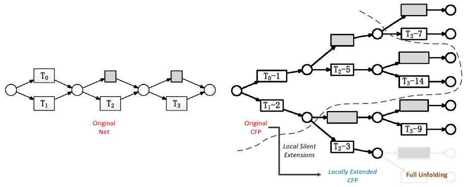
Refer to caption
Figure 8: Merged continued CFPs can be as large as the reachability graph.

In such cases, we may re-use existing structures in CFP as an isomorphism of the behavior after cut-off events. Next, we show that this can be realized by redirecting the post-arcs of some cut-off events. The basic purpose is to ‘link’ the cut-off events back to the existing nodes in the CFP. Actually, we may do this when the cut-off events have identical ‘context’ with its corresponding event, as the following definition shows.

Definition 5.5 (Contextual Isomorphism and Redirected CFP)

In an unfolding prefix π𝜋\pi, let e𝑒e be a cut-off event and esuperscript𝑒e^{\prime} its corresponding event such that esuperscript𝑒e^{\prime} is not a cut-off event. Let γ:eCut([e])\gamma:e\bullet\rightarrow Cut([e^{\prime}]) denote an injective mapping from ee\bullet to the conditions in Cut([e])𝐶𝑢𝑡delimited-[]superscript𝑒Cut([e^{\prime}]). If there exists a mapping γ𝛾\gamma such that

  • (1)

    h(c)=h(γ(c)),ceh(c)=h(\gamma(c)),c\in e\bullet, and

  • (2)

    ce,c(eγ(e)):c\forall c\in e\bullet,c^{\prime}\not\in(e\bullet\cup\gamma(e\bullet)):c^{\prime} co cc𝑐superscript𝑐c\Leftrightarrow c^{\prime} co γ(c)𝛾𝑐\gamma(c).

we say that e𝑒e is contextually isomorphic with esuperscript𝑒e^{\prime} under the mapping γ𝛾\gamma (denoted as eγesuperscriptsimilar-to𝛾𝑒superscript𝑒e\stackrel{{\scriptstyle\gamma}}{{\sim}}e^{\prime}).

Note that the above properties are not implied by the definition of cut-off events, which only guarantees Cut([e])𝐶𝑢𝑡delimited-[]𝑒Cut([e]) and Cut([e])𝐶𝑢𝑡delimited-[]superscript𝑒Cut([e^{\prime}]) are mapped to identical set of places. However, we notice they can be applied for most of the cut-off events in the practical models.

When a cut-off event e𝑒e is contextually isomorphic with some esuperscript𝑒e^{\prime}, we can ‘link’ e𝑒e towards the conditions in Cut([e])𝐶𝑢𝑡delimited-[]superscript𝑒Cut([e^{\prime}]) according to the γ𝛾\gamma mapping so as to reuse the existing structure after Cut([e])𝐶𝑢𝑡delimited-[]superscript𝑒Cut([e^{\prime}]). For every condition c𝑐c in ee\bullet, we redirect the arc following e𝑒e from their original target condition c𝑐c to γ(c)𝛾𝑐\gamma(c), and we call these arcs redirected arcs. After that, we remove the original conditions in ee\bullet from the CFP. Note that the redirected arcs introduced should not be taken as the same as the original arcs in the unfolding, otherwise, they will disrupt the restriction of branching process that |c|1|\bullet c|\leq 1, and it may also disrupt the acyclic property of the original causal relation ‘<<’. Therefore the redirected arcs are used separately for pTAR derivation only. We use pre(c)𝑝𝑟𝑒𝑐pre(c) to denote the set of starting events whose post-arcs are redirected to a condition c𝑐c, which is defined as:

pre(c)={eπ|ce,eπ:eγeγ(c)=c}pre(c)=\{e\in\pi|\exists c^{\prime}\in e\bullet,e^{\prime}\in\pi:e\stackrel{{\scriptstyle\gamma}}{{\sim}}e^{\prime}\wedge\gamma(c^{\prime})=c\}

Intuitively, we could call the events in pre(c)𝑝𝑟𝑒𝑐pre(c), whose post-arcs are redirected, as ‘soft’ cut-off events. We denote the redirected CFP of the original CFP π𝜋\pi as (π\Ec,pre)(\pi\backslash E_{c}\bullet,pre), where Ecsubscript𝐸𝑐E_{c} is the set of ‘soft’ cut-off events and pre𝑝𝑟𝑒pre indicates the redirected arc relations.

In the following example, we could see that the truncated behaviors after cut-off event T2-4subscript𝑇2-4T_{2}\mbox{-}4 and the two silent events are consecutively continued after the conditions which redirected arcs point to. We call such events soft𝑠𝑜𝑓𝑡soft cut-off events because we can find their succeeding behaviors by contextual isomorphism without performing further local extensions.
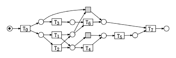
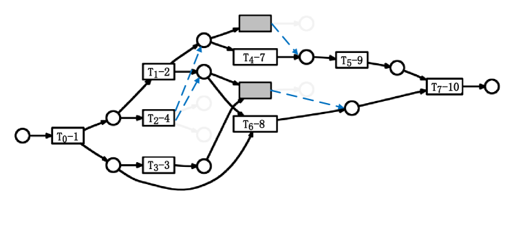
Refer to caption
(a)
Refer to caption
(b)
Figure 9: Illustration of ‘soft’ cut-off events

Note that contextual isomorphism differs from the original isomorphism, i.e. the property mentioned and used by McMillan and Esparza in [18] and [17]. The previous isomorphism cannot guarantee the partial silent adjacency structures starting from e𝑒e can be immediately continued after [e]absentdelimited-[]superscript𝑒\Uparrow[e^{\prime}], since other cut-off events in [e]absentdelimited-[]superscript𝑒\Uparrow[e^{\prime}] might have prevented the unfolding of corresponding continued silent adjacency structures in the original CFP.

Compared to the previous isomorphism [17], contextual isomorphism puts additional constraints on the co-sets ‘near’ the cut-off events. With these additional constraints, it ensures that we can look for the isomorphic silent adjacency structures. Thus, less local extensions are required.

Definition 5.6 (Redirected Silent Adjacency)

For an ordered pair of nodes n1,n2subscript𝑛1subscript𝑛2\langle n_{1},n_{2}\rangle in a redirected CFP, they are in redirected silent adjacency, denoted as n1sn2subscriptsuperscript𝑠subscript𝑛1subscript𝑛2n_{1}\triangleright^{\prime}_{s}n_{2}, if and only if one of the following conditions holds:

  • (1)

    n1n2n_{1}\in\bullet n_{2}, or

  • (2)

    n2subscript𝑛2n_{2} is a condition, en2pre(n2):n1se\exists e\in\bullet n_{2}\cup pre(n_{2}):n_{1}\triangleright_{s}^{\prime}e and h(e)𝑒h(e) is a silent transition, or

  • (3)

    n2subscript𝑛2n_{2} is an event, and cn2:n1scn1\forall c\in\bullet n_{2}:n_{1}\triangleright_{s}^{\prime}c\vee n_{1} co c𝑐c.

Algorithm 4 Derive All pTARs from a Net System Using Redirected CFPs
1:function DerivePTARs(S,π0𝑆subscript𝜋0S,\pi_{0})
2:     pTAR𝑝𝑇𝐴𝑅pTAR\leftarrow\emptyset
3:     Extended𝐸𝑥𝑡𝑒𝑛𝑑𝑒𝑑Extended\leftarrow\emptyset
4:     ππ0𝜋subscript𝜋0\pi\leftarrow\pi_{0}
5:     for each cut-off event ecπ0subscript𝑒𝑐subscript𝜋0e_{c}\in\pi_{0} do
6:     if e:ee:not-existssuperscript𝑒similar-to𝑒superscript𝑒\not\exists e^{\prime}:e\sim e^{\prime} then hard-cut-off\leftarrow hard-cut-off {e}superscript𝑒\cup\{e^{\prime}\}
7:     else for each ecπ:ecec:subscriptsuperscript𝑒𝑐𝜋similar-tosubscriptsuperscript𝑒𝑐subscript𝑒𝑐e^{\prime}_{c}\in\pi:e^{\prime}_{c}\sim e_{c} do
8:     for each cecc\in e_{c}\bullet do ππ{ec,γ(c)}𝜋𝜋subscript𝑒𝑐𝛾𝑐\pi\leftarrow\pi\cup\{\langle e_{c},\gamma(c)\rangle\}
9:     for each e1,e2π:e1se2:subscript𝑒1subscript𝑒2𝜋subscript𝑠subscript𝑒1subscript𝑒2e_{1},e_{2}\in\pi:e_{1}\triangleright_{s}e_{2} do
10:     pTARpTARh(e1),h(e2)𝑝𝑇𝐴𝑅𝑝𝑇𝐴𝑅subscript𝑒1subscript𝑒2pTAR\leftarrow pTAR\cup\langle h(e_{1}),h(e_{2})\rangle
11:     for each ecsubscript𝑒𝑐absente_{c}\in hard-cut-off do
12:     for each e1π:e1sec:subscript𝑒1𝜋subscript𝑠subscript𝑒1subscript𝑒𝑐e_{1}\in\pi:e_{1}\triangleright_{s}e_{c} do
13:     if e1Extendedsubscript𝑒1𝐸𝑥𝑡𝑒𝑛𝑑𝑒𝑑e_{1}\not\in Extended then
14:     ExtendedExtended{e1}𝐸𝑥𝑡𝑒𝑛𝑑𝑒𝑑𝐸𝑥𝑡𝑒𝑛𝑑𝑒𝑑subscript𝑒1Extended\leftarrow Extended\cup\{e_{1}\}
15:     Fine1=FinitePrefixForPTAR(S,π,e1)𝐹𝑖subscript𝑛subscript𝑒1FinitePrefixForPTAR𝑆𝜋subscript𝑒1Fin_{e_{1}}=\textsc{FinitePrefixForPTAR}(S,\pi,e_{1})
16:     for each ea,eb:ebFine1\π,easeb:subscript𝑒𝑎subscript𝑒𝑏subscript𝑒𝑏\𝐹𝑖subscript𝑛subscript𝑒1𝜋superscriptsubscript𝑠subscript𝑒𝑎subscript𝑒𝑏e_{a},e_{b}:e_{b}\in Fin_{e_{1}}\backslash\pi,e_{a}\triangleright_{s}^{\prime}e_{b} do
17:     pTARpTARh(ea),h(eb)𝑝𝑇𝐴𝑅𝑝𝑇𝐴𝑅subscript𝑒𝑎subscript𝑒𝑏pTAR\leftarrow pTAR\cup\langle h(e_{a}),h(e_{b})\rangle
18:     ππFine1𝜋𝜋𝐹𝑖subscript𝑛subscript𝑒1\pi\leftarrow\pi\cup Fin_{e_{1}}
19:     end if
20:     return pTAR𝑝𝑇𝐴𝑅pTAR
21:end function

It is easy to see that the above definition of ssuperscriptsubscript𝑠\triangleright_{s}^{\prime} is equivalent with the original ssubscript𝑠\triangleright_{s} within the original CFP π𝜋\pi. The major difference lies in (2), for not only the original causal relations but also the redirected arcs represented by pre(c)𝑝𝑟𝑒𝑐pre(c) are taken into account while backtracking. In redirected CFPs, we need only replace the ssubscript𝑠\triangleright_{s} in Algorithm 12 in the last section with ssuperscriptsubscript𝑠\triangleright_{s}^{\prime} and we can get the pTAR derivation algorithms for redirected CFPs. So a pTAR computing algorithm using redirected CFP can now be given as Algorithm 4, for which the original net S𝑆S its CFP π0subscript𝜋0\pi_{0} are assumed to be given as input.

Theorem 5.5

For two transitions t1,t2subscript𝑡1subscript𝑡2t_{1},t_{2} t1<ptart2subscript𝑝𝑡𝑎𝑟subscript𝑡1subscript𝑡2t_{1}<_{ptar}t_{2} if and only if there exists e1,e2:h(e1)=t1,h(e2)=t2:subscript𝑒1subscript𝑒2formulae-sequencesubscript𝑒1subscript𝑡1subscript𝑒2subscript𝑡2e_{1},e_{2}:h(e_{1})=t_{1},h(e_{2})=t_{2} such that e1π,e2μ(π\Ec)e_{1}\in\pi,e_{2}\in\mu(\pi\backslash E_{c}\bullet) and e1se2superscriptsubscript𝑠subscript𝑒1subscript𝑒2e_{1}\triangleright_{s}^{\prime}e_{2}.

Proof:

(\Rightarrow)By Theorem 5.4, for the original CFP π𝜋\pi, there exists e1π,e2βe1μ(π)formulae-sequencesubscript𝑒1𝜋subscriptsuperscript𝑒2subscript𝛽subscript𝑒1𝜇𝜋e_{1}\in\pi,e^{\prime}_{2}\in\beta_{e_{1}}\subseteq\mu(\pi) such that h(e1)=t1,h(e2)=t2formulae-sequencesubscript𝑒1subscript𝑡1subscript𝑒2subscript𝑡2h(e_{1})=t_{1},h(e_{2})=t_{2} and e1se2subscript𝑠subscript𝑒1subscript𝑒2e_{1}\triangleright_{s}e_{2}. Since in the original π𝜋\pi, ssuperscriptsubscript𝑠\triangleright_{s}^{\prime} and ssubscript𝑠\triangleright_{s} is equivalent, the case when e2πsubscript𝑒2𝜋e_{2}\in\pi is trivial. Therefore we only focus on the cases when [e2]\π\delimited-[]subscript𝑒2𝜋[e_{2}]\backslash\pi\neq\emptyset.

(1) Consider the set of events Eext=[e2]\πsubscript𝐸𝑒𝑥𝑡\delimited-[]subscript𝑒2𝜋E_{ext}=[e_{2}]\backslash\pi and its minimal conditions Cmin=Min(Ec)C_{min}=Min(\bullet E_{c}). Without loss of generality, let Eext={em1,em2,,emk,e2}subscript𝐸𝑒𝑥𝑡subscript𝑒subscript𝑚1subscript𝑒subscript𝑚2subscript𝑒subscript𝑚𝑘subscript𝑒2E_{ext}=\{e_{m_{1}},e_{m_{2}},...,e_{m_{k}},e_{2}\}, where emi<emji<jsubscript𝑒subscript𝑚𝑖subscript𝑒subscript𝑚𝑗𝑖𝑗e_{m_{i}}<e_{m_{j}}\rightarrow i<j. Since Cminπ\EcC_{min}\subseteq\pi\backslash E_{c}\bullet, then since sssubscript𝑠superscriptsubscript𝑠\triangleright_{s}\subseteq\triangleright_{s}^{\prime}, we have Eextμ(π\Ec)E_{ext}\subseteq\mu(\pi\backslash E_{c}\bullet) and therefore the proposition holds.

(2) If Cminπ\EcC_{min}\not\subseteq\pi\backslash E_{c}\bullet, then the pre-events of the conditions in Cmin\(π\Ec)C_{min}\backslash(\pi\backslash E_{c}\bullet) are redirected due to contextual isomorphism. Given property (2) of context isomorphism, the new conditions they link to still form a co-set Cminsubscriptsuperscript𝐶𝑚𝑖𝑛C^{\prime}_{min} isomorphic with Cminsubscript𝐶𝑚𝑖𝑛C_{min} and cCmin:e1sc:for-all𝑐subscriptsuperscript𝐶𝑚𝑖𝑛superscriptsubscript𝑠subscript𝑒1𝑐\forall c\in C^{\prime}_{min}:e_{1}\triangleright_{s}^{\prime}c. By isomorphism, a sequence of events Eext={em1,}superscriptsubscript𝐸𝑒𝑥𝑡subscriptsuperscript𝑒subscript𝑚1E_{ext}^{\prime}=\{e^{\prime}_{m_{1}},...\} (|Eext|1superscriptsubscript𝐸𝑒𝑥𝑡1|E_{ext}^{\prime}|\geq 1) isomorphic with a prefix of Eext={em1,em2,,emk,e2}subscript𝐸𝑒𝑥𝑡subscript𝑒subscript𝑚1subscript𝑒subscript𝑚2subscript𝑒subscript𝑚𝑘subscript𝑒2E_{ext}=\{e_{m_{1}},e_{m_{2}},...,e_{m_{k}},e_{2}\} could be found after Cminsubscriptsuperscript𝐶𝑚𝑖𝑛C^{\prime}_{min} until cut-off events are encountered, and it is easy to prove that e1semisuperscriptsubscript𝑠subscript𝑒1subscriptsuperscript𝑒subscript𝑚𝑖e_{1}\triangleright_{s}^{\prime}e^{\prime}_{m_{i}}. If Eextsuperscriptsubscript𝐸𝑒𝑥𝑡E_{ext}^{\prime} does not contain any cut-off event, then it will correspond to the full sequence of Eextsubscript𝐸𝑒𝑥𝑡E_{ext}, and the proposition already holds. Otherwise, without loss of generality, suppose Eext={em1,,emp}superscriptsubscript𝐸𝑒𝑥𝑡subscriptsuperscript𝑒subscript𝑚1subscriptsuperscript𝑒subscript𝑚𝑝E_{ext}^{\prime}=\{e^{\prime}_{m_{1}},...,e^{\prime}_{m_{p}}\}. Let Cmin′′=(Cmin\Eext)EextC^{\prime\prime}_{min}=(C^{\prime}_{min}\backslash\bullet E_{ext}^{\prime})\cup E_{ext}^{\prime}\bullet. If Cmin′′(π\Ec)C^{\prime\prime}_{min}\subseteq(\pi\backslash E_{c}\bullet), then by the same reasoning in Thm. 5.4 and (1), after Cmin′′subscriptsuperscript𝐶′′𝑚𝑖𝑛C^{\prime\prime}_{min}, a sequence with the form of {emp+1,,e2},h(e2)=t2subscriptsuperscript𝑒subscript𝑚𝑝1subscriptsuperscript𝑒2subscriptsuperscript𝑒2subscript𝑡2\{e^{\prime}_{m_{p+1}},...,e^{\prime}_{2}\},h(e^{\prime}_{2})=t_{2}, can be found by performing local silent extensions such that e1se2,e2μ(π\Ec)e_{1}\triangleright_{s}^{\prime}e^{\prime}_{2},e^{\prime}_{2}\in\mu(\pi\backslash E_{c}\bullet). If Cmin′′(π\Ec)C^{\prime\prime}_{min}\not\subseteq(\pi\backslash E_{c}\bullet), we could iterate (2) again from Cmin′′subscriptsuperscript𝐶′′𝑚𝑖𝑛C^{\prime\prime}_{min}. Since Eextsubscript𝐸𝑒𝑥𝑡E_{ext} is finite, the iteration cannot be repeated infinitely, so we will eventually arrive at some e2μ(π\Ec)e_{2}^{\prime}\in\mu(\pi\backslash E_{c}\bullet).

Let Ep={e|ec,cCmin}E_{p}=\{e|e\in\bullet c,c\in C_{min}\}. Since cCmin:e1sc:for-all𝑐subscript𝐶𝑚𝑖𝑛subscript𝑠subscript𝑒1𝑐\forall c\in C_{min}:e_{1}\triangleright_{s}c, we know that epEp:e1sc:for-allsubscript𝑒𝑝subscript𝐸𝑝subscript𝑠subscript𝑒1𝑐\forall e_{p}\in E_{p}:e_{1}\triangleright_{s}c.

Let ErCminE_{r}\subseteq\bullet C_{min} be the set of events that are redirected in the pre-events of the conditions in Cminsubscript𝐶𝑚𝑖𝑛C_{min}. Given property (2) of context equivalence, even if some pre-events of Cminsubscript𝐶𝑚𝑖𝑛C_{min} not included in EMsubscript𝐸𝑀E_{M} are redirected in πsuperscript𝜋\pi^{\prime}, the new conditions they link to still form a co-set Cminsubscriptsuperscript𝐶𝑚𝑖𝑛C^{\prime}_{min} in πsuperscript𝜋\pi^{\prime} that is isomorphic with Cminsubscript𝐶𝑚𝑖𝑛C_{min} and cCmin:e1c:for-all𝑐subscriptsuperscript𝐶𝑚𝑖𝑛subscript𝑒1𝑐\forall c\in C^{\prime}_{min}:e_{1}\triangleright c. Starting from Cminsubscriptsuperscript𝐶𝑚𝑖𝑛C^{\prime}_{min}, we can find an event e2subscript𝑒2e_{2} either through local silent extensions in μ(π)𝜇superscript𝜋\mu(\pi^{\prime}) (by Proposition X) or as existing event in πsuperscript𝜋\pi^{\prime}, such that e2μ(π)subscriptsuperscript𝑒2𝜇superscript𝜋e^{\prime}_{2}\in\mu(\pi^{\prime}) and e1se2subscript𝑠subscript𝑒1subscriptsuperscript𝑒2e_{1}\triangleright_{s}e^{\prime}_{2}

Since only the events in EMπsubscript𝐸𝑀𝜋E_{M}\cap\pi can be redirected, and only the events in EM\π\subscript𝐸𝑀𝜋E_{M}\backslash\pi would affected, the case of EMπsubscript𝐸𝑀𝜋E_{M}\subseteq\pi is trivial. We now consider the case when EM\π\subscript𝐸𝑀𝜋E_{M}\backslash\pi\neq\emptyset.

(1) If none of the events in EMπsubscript𝐸𝑀𝜋E_{M}\cap\pi has been redirected in πsuperscript𝜋\pi^{\prime}. Consider the set of conditions Cmin=Min((EM\π))C_{min}=Min(\bullet(E_{M}\backslash\pi)) in the original π𝜋\pi, and from e1se2subscript𝑠subscript𝑒1subscript𝑒2e_{1}\triangleright_{s}e_{2} we have cCmin:e1c:for-all𝑐subscript𝐶𝑚𝑖𝑛subscript𝑒1𝑐\forall c\in C_{min}:e_{1}\triangleright c. Given property (2) of context equivalence, even if some pre-events of Cminsubscript𝐶𝑚𝑖𝑛C_{min} not included in EMsubscript𝐸𝑀E_{M} are redirected in πsuperscript𝜋\pi^{\prime}, the new conditions they link to still form a co-set Cminsubscriptsuperscript𝐶𝑚𝑖𝑛C^{\prime}_{min} in πsuperscript𝜋\pi^{\prime} that is isomorphic with Cminsubscript𝐶𝑚𝑖𝑛C_{min} and cCmin:e1c:for-all𝑐subscriptsuperscript𝐶𝑚𝑖𝑛subscript𝑒1𝑐\forall c\in C^{\prime}_{min}:e_{1}\triangleright c. Starting from Cminsubscriptsuperscript𝐶𝑚𝑖𝑛C^{\prime}_{min}, we can find an event e2subscript𝑒2e_{2} either through local silent extensions in μ(π)𝜇superscript𝜋\mu(\pi^{\prime}) (by Proposition X) or as existing event in πsuperscript𝜋\pi^{\prime}, such that e2μ(π)subscriptsuperscript𝑒2𝜇superscript𝜋e^{\prime}_{2}\in\mu(\pi^{\prime}) and e1se2subscript𝑠subscript𝑒1subscriptsuperscript𝑒2e_{1}\triangleright_{s}e^{\prime}_{2}.

(2) Suppose some emisubscript𝑒subscript𝑚𝑖e_{m_{i}} in EMπsubscript𝐸𝑀𝜋E_{M}\cap\pi has been redirected in πsuperscript𝜋\pi^{\prime}. Then since either emi<emi+1subscript𝑒subscript𝑚𝑖subscript𝑒subscript𝑚𝑖1e_{m_{i}}<e_{m_{i+1}} or emisubscript𝑒subscript𝑚𝑖e_{m_{i}} co emi+1subscript𝑒subscript𝑚𝑖1e_{m_{i+1}}, by property (2) of Def. X, we know that in the redirect CFP πsuperscript𝜋\pi^{\prime}, some event emi+1:h(emi+1)=h(emi+1):superscriptsubscript𝑒subscript𝑚𝑖1superscriptsubscript𝑒subscript𝑚𝑖1subscript𝑒subscript𝑚𝑖1e_{m_{i+1}}^{\prime}:h(e_{m_{i+1}}^{\prime})=h(e_{m_{i+1}}) and obviously e1semi+1subscript𝑠subscript𝑒1superscriptsubscript𝑒subscript𝑚𝑖1e_{1}\triangleright_{s}e_{m_{i+1}}^{\prime}. If emi+1superscriptsubscript𝑒subscript𝑚𝑖1e_{m_{i+1}}^{\prime} is not a cut-off event, then we can find in πsuperscript𝜋\pi^{\prime} an emi+2superscriptsubscript𝑒subscript𝑚𝑖2e_{m_{i+2}}^{\prime} which is isomorphic with emi+2subscript𝑒subscript𝑚𝑖2e_{m_{i+2}} and e1semi+2subscript𝑠subscript𝑒1superscriptsubscript𝑒subscript𝑚𝑖2e_{1}\triangleright_{s}e_{m_{i+2}}^{\prime}. This can be iterated until we reach some event isomorphic with e2subscript𝑒2e_{2}, which proves the proposition, or some emjsuperscriptsubscript𝑒subscript𝑚𝑗e_{m_{j}}^{\prime} that is a cut-off event. If emjsuperscriptsubscript𝑒subscript𝑚𝑗e_{m_{j}}^{\prime} is not redirected, then by the property of contextual equivalence and Prop. X, an event e2subscriptsuperscript𝑒2e^{\prime}_{2} after emjsuperscriptsubscript𝑒subscript𝑚𝑗e_{m_{j}}^{\prime} can be discovered through local silent extensions such that e2μ(π)subscriptsuperscript𝑒2𝜇superscript𝜋e^{\prime}_{2}\in\mu(\pi^{\prime}) and e1se2subscript𝑠subscript𝑒1subscriptsuperscript𝑒2e_{1}\triangleright_{s}e^{\prime}_{2}. If emjsuperscriptsubscript𝑒subscript𝑚𝑗e_{m_{j}}^{\prime} is redirected, then we can iterate the process of (2). This iteration cannot continue infinitely because EMsubscript𝐸𝑀E_{M} is finite, and eventually we will arrive at e2μ(π)subscriptsuperscript𝑒2𝜇superscript𝜋\exists e^{\prime}_{2}\in\mu(\pi^{\prime}) and e1se2,h(e1)=t1subscript𝑠subscript𝑒1subscriptsuperscript𝑒2subscript𝑒1subscript𝑡1e_{1}\triangleright_{s}e^{\prime}_{2},h(e_{1})=t_{1} and h(e2)=t2subscriptsuperscript𝑒2subscript𝑡2h(e^{\prime}_{2})=t_{2}.

\Leftarrow) Given that e1se2superscriptsubscript𝑠subscript𝑒1subscript𝑒2e_{1}\triangleright_{s}^{\prime}e_{2}, consider the co-set B0=e2B_{0}=\bullet e^{\prime}_{2}. As ce2:c\forall c\in\bullet e_{2}:c co e1subscript𝑒1e_{1} or e1scsuperscriptsubscript𝑠subscript𝑒1𝑐e_{1}\triangleright_{s}^{\prime}c, let B0co={cB0B_{0_{co}}=\{c\in B_{0} co e1}e_{1}\}, B0prec={cB0|e1sc}subscript𝐵subscript0𝑝𝑟𝑒𝑐conditional-set𝑐subscript𝐵0superscriptsubscript𝑠subscript𝑒1𝑐B_{0_{prec}}=\{c\in B_{0}|e_{1}\triangleright_{s}^{\prime}c\}. Obviously B0=B0coB0precsubscript𝐵0subscript𝐵subscript0𝑐𝑜subscript𝐵subscript0𝑝𝑟𝑒𝑐B_{0}=B_{0_{co}}\cup B_{0_{prec}}.

Take any condition csuperscript𝑐c^{\prime} from B0precsubscript𝐵subscript0𝑝𝑟𝑒𝑐B_{0_{prec}}, since e1scsuperscriptsubscript𝑠subscript𝑒1superscript𝑐e_{1}\triangleright_{s}^{\prime}c^{\prime}, it follows that ekcprec(c):e1sek}\exists e_{k}\in\bullet c^{\prime}\cup prec(c^{\prime}):e_{1}\triangleright_{s}^{\prime}e_{k}\} and h(ek)subscript𝑒𝑘h(e_{k}) is a silent transition.

If ek<csubscript𝑒𝑘superscript𝑐e_{k}<c^{\prime}, then let B1=(B0\ek)ekB_{1}=(B_{0}\backslash e_{k}\bullet)\cup\bullet e_{k}. We have eksubscript𝑒𝑘e_{k} co B0\ekB_{0}\backslash e_{k}\bullet (obviously ek<csubscript𝑒𝑘superscript𝑐e_{k}<c^{\prime} cannot hold, and for any cB0\ekc^{\prime}\in B_{0}\backslash e_{k}\bullet, if ek#cc<eksubscript𝑒𝑘#𝑐𝑐subscript𝑒𝑘e_{k}\#c\vee c<e_{k}, it will lead to a contradiction with the fact that B0subscript𝐵0B_{0} is a co-set). We can prove that ekabsentsubscript𝑒𝑘\bullet e_{k} are in co𝑐𝑜co with B0\ekB_{0}\backslash e_{k}\bullet (for any c′′e,cB0\ekc^{\prime\prime}\in\bullet e,c^{\prime}\in B_{0}\backslash e_{k}\bullet, any one of c′′#csuperscript𝑐′′#superscript𝑐c^{\prime\prime}\#c^{\prime}, c′′<csuperscript𝑐′′superscript𝑐c^{\prime\prime}<c^{\prime} or c<c′′superscript𝑐superscript𝑐′′c^{\prime}<c^{\prime\prime} would lead to the contradiction with the fact that eksubscript𝑒𝑘e_{k} co csuperscript𝑐c^{\prime}) and consequently B1=(B0\ek)ekB_{1}=(B_{0}\backslash e_{k}\bullet)\cup\bullet e_{k} is a co-set.

If ekprec(c)subscript𝑒𝑘𝑝𝑟𝑒𝑐superscript𝑐e_{k}\in prec(c^{\prime}) then let B1=(B0\pre1(ek))ekB_{1}=(B_{0}\backslash pre^{-1}(e_{k}))\cup\bullet e_{k}. In the original π𝜋\pi, by the property (2) of Def. 5.5, as eke_{k}\bullet have isomorphic context with pre1(ek)𝑝𝑟superscript𝑒1subscript𝑒𝑘pre^{-1}(e_{k}), we can similarly prove that eksubscript𝑒𝑘e_{k} are in co𝑐𝑜co with B0\pre1(ek)\subscript𝐵0𝑝𝑟superscript𝑒1subscript𝑒𝑘B_{0}\backslash pre^{-1}(e_{k}). Consequently, ekabsentsubscript𝑒𝑘\bullet e_{k} are in co𝑐𝑜co with B0\pre1(ek)\subscript𝐵0𝑝𝑟superscript𝑒1subscript𝑒𝑘B_{0}\backslash pre^{-1}(e_{k}) and therefore B1=(B0\pre1(ek))ekB_{1}=(B_{0}\backslash pre^{-1}(e_{k}))\cup\bullet e_{k} is a co-set. In both cases B1subscript𝐵1B_{1} is a co-set Similarly, we could have B1co={cB1B_{1_{co}}=\{c\in B_{1} co e1}e_{1}\}, B1prec={cB1|e1sc}subscript𝐵subscript1𝑝𝑟𝑒𝑐conditional-set𝑐subscript𝐵1superscriptsubscript𝑠subscript𝑒1𝑐B_{1_{prec}}=\{c\in B_{1}|e_{1}\triangleright_{s}^{\prime}c\}.

In both cases, we could generate from B0subscript𝐵0B_{0} a new co-set B1subscript𝐵1B_{1} such that eksubscript𝑒𝑘e_{k} is enabled at some reachable marking Mksubscript𝑀𝑘M_{k} that contains h(B1)subscript𝐵1h(B_{1}), and the firing of h(ek)subscript𝑒𝑘h(e_{k}) from that reachable marking will lead to a reachable marking Mk+1subscript𝑀𝑘1M_{k+1} that contains B0subscript𝐵0B_{0} and therefore enables h(e2)subscript𝑒2h(e_{2}), which gives Mkh(ek)Mk+1subscript𝑒𝑘subscript𝑀𝑘subscript𝑀𝑘1M_{k}\xrightarrow{h(e_{k})}M_{k+1}, and h(e2)subscript𝑒2h(e_{2}) is enabled at Mk+1subscript𝑀𝑘1M_{k+1}.

Again, since e1seksuperscriptsubscript𝑠subscript𝑒1subscript𝑒𝑘e_{1}\triangleright_{s}^{\prime}e_{k}, we have cek:c\forall c\in\bullet e_{k}:c co e1subscript𝑒1e_{1} or e1scsuperscriptsubscript𝑠subscript𝑒1𝑐e_{1}\triangleright_{s}^{\prime}c. Therefore, as B1\B0=ekB_{1}\backslash B_{0}=\bullet e_{k}, we have cB1:c\forall c\in\bullet B_{1}:c co e1subscript𝑒1e_{1} or e1scsuperscriptsubscript𝑠subscript𝑒1𝑐e_{1}\triangleright_{s}^{\prime}c. Again, we can partition B1subscript𝐵1B_{1} as B1co={cB1B_{1_{co}}=\{c\in B_{1} co e1}e_{1}\} and B1prec={cB1|e1sc}subscript𝐵subscript1𝑝𝑟𝑒𝑐conditional-set𝑐subscript𝐵1superscriptsubscript𝑠subscript𝑒1𝑐B_{1_{prec}}=\{c\in B_{1}|e_{1}\triangleright_{s}^{\prime}c\} (B1=B1coB1precsubscript𝐵1subscript𝐵subscript1𝑐𝑜subscript𝐵subscript1𝑝𝑟𝑒𝑐B_{1}=B_{1_{co}}\cup B_{1_{prec}}). Take any condition c𝑐c from B1precsubscript𝐵subscript1𝑝𝑟𝑒𝑐B_{1_{prec}}, and we can repeat the above iterations to find the next event ek1subscript𝑒𝑘1e_{k-1} such that h(ek1)subscript𝑒𝑘1h(e_{k-1}) is a silent transition and Mk1h(ek1)Mkh(ek)Mk+1subscript𝑒𝑘1subscript𝑀𝑘1subscript𝑀𝑘subscript𝑒𝑘subscript𝑀𝑘1M_{k-1}\xrightarrow{h(e_{k-1})}M_{k}\xrightarrow{h(e_{k})}M_{k+1}. Since μ(π)𝜇𝜋\mu(\pi) is finite, we could arrive with finite steps at e1subscript𝑒1e_{1} and M1h(e1)Mkh(ek)Mk+1subscript𝑒1subscript𝑀1subscript𝑀𝑘subscript𝑒𝑘subscript𝑀𝑘1M_{1}\xrightarrow{h(e_{1})}...M_{k}\xrightarrow{h(e_{k})}M_{k+1} and h(e2)subscript𝑒2h(e_{2}) is enabled at Mk+1subscript𝑀𝑘1M_{k+1}. Therefore we have h(e1)<ptarh(e2)subscript𝑝𝑡𝑎𝑟subscript𝑒1subscript𝑒2h(e_{1})<_{ptar}h(e_{2}).

In case (1) let B0={cB0|cemk}B_{0}^{\prime}=\{c\in B_{0}|c\in e_{m_{k}}\bullet\}. Since emkse2superscriptsubscript𝑠subscript𝑒subscript𝑚𝑘subscript𝑒2e_{m_{k}}\triangleright_{s}^{\prime}e_{2} and emi<emji<jsubscript𝑒subscript𝑚𝑖subscript𝑒subscript𝑚𝑗𝑖𝑗e_{m_{i}}<e_{m_{j}}\rightarrow i<j, we can easily prove that Bk1=(Bk\Bk)emkB_{k-1}=(B_{k}\backslash B^{\prime}_{k})\cup\bullet e_{m_{k}} is a co-set, and h(emk)subscript𝑒subscript𝑚𝑘h(e_{m_{k}}) is ‘enabled’ at any reachable marking Mksubscript𝑀𝑘M_{k} containing h(Bk1)subscript𝐵𝑘1h(B_{k-1}). And since BkemkB^{\prime}_{k}\subseteq e_{m_{k}}\bullet, the firing h(emk)subscript𝑒subscript𝑚𝑘h(e_{m_{k}})

In case (2) let B0={cB0|emkpre(c)}superscriptsubscript𝐵0conditional-set𝑐subscript𝐵0subscript𝑒subscript𝑚𝑘𝑝𝑟𝑒𝑐B_{0}^{\prime}=\{c\in B_{0}|e_{m_{k}}\in pre(c)\}. By property (2) of Def. X, we can also easily prove that Bk1=(Bk\Bk)emkB_{k-1}=(B_{k}\backslash B^{\prime}_{k})\cup\bullet e_{m_{k}} is a co-set, and h(ek)subscript𝑒𝑘h(e_{k}) is ‘enabled’ at any reachable marking containing h(Bk1)subscript𝐵𝑘1h(B_{k-1}).

In Algorithm 4, since we can re-use existing CFP structures to observe behaviors after soft cut-off events, significant amount of computational costs can be reduced, as will be demonstrated with detailed performance analysis in the experiment section.

6 Performance Evaluation

6.1 TAR Computing Performance

We conduct experiments to evaluate the effectiveness of our proposed CFP-based algorithms using both industrial (see [20] for further details) and artificial process model datasets. We have implemented our algorithms based on the open source BPM tool jBPT111http://code.google.com/p/jbpt and all our programs and the process model datasets have been made available on-line222http://laudms.thss.tsinghua.edu.cn/trac/Test/raw-attachment/wiki/Share/CTAR.zip. All experiments were run on a PC with Intel Dual Core I5 CPU@2.8G, 4G DDR3@1333MHz, and Windows 7 Enterprise OS. For simplicity, we focus on the TAR computing performance in this experiment, as many existing algorithms do not support pTAR computation. But still, this could demonstrate the performance improvement of our accelerated method (IMPROVE) against the baseline coverability based method (GENERAL) and other existing methods, since clearly the improvement in pTAR computing performance, if there is any, will only be greater than that of TAR.

6.1.1 Real-world Data

Table 2 summarizes the features of our experiment datasets [20] consisting of 5 libraries, from which we extract all the bounded models for evaluation. The table also shows the degree of concurrency found in the process models, i.e. the maximum and average number of tokens that occur in a single reachable non-error state of the process. Since RG-based algorithms may encounter state-explosions when applied on nets with high concurrencies, we count the target net as “Time Limit Exceeded for RG” if it fails to construct a RG within acceptable time limit, as shown in the last row of the table.

TABLE I: Features of the five process model libraries used in experiments
A2 B2 B3 B4 M1
Num. of Bounded Nets 256 392 338 272 27
Avg. Transitions/Places 28/44 29/43 27/41 28/41 48/45
Avg./Max Concurrency 2/13 8/14 16/66 14/33 2/4
Time-Limit Exceeded for RG 0 39 36 24 3

First, we compare the time costs (see Fig. 10a) of our algorithm GENERAL (Algorithm 1) which is based on coverability reduction against Jin’s approach (JIN) based on the primitive unfolding derivation rules in [8] (which does not support arbitrary bounded nets since it assumes free-choice WF-nets), and two RG-based algorithms (pure RG-based algorithm in [2] (RG) and Zha’s improved RG based approach (ZHA) [1]). Time costs of building CFPs of unfoldings alone (CFP-BUILD) in each library are also shown in Fig. 10a. It can be observed that as nets in B2, B3 and B4 contain more concurrent structures, GENERAL performs significantly better than all RG-based algorithms while only being a bit slower than RG in A2, M1, which can be explained by the lacking of concurrent structures in these two libraries. By comparing their overall time cost (TOTAL), we observe that GENERAL is around 11.98 times and 9.78 times faster than RG and ZHA respectively. We also see that whereas JIN only supports sound and free-choice nets, our GENERAL achieves a much greater generality (supports any bounded net system) at the expense of only a bit more overhead and shows comparable performance with JIN (only 1.1% more time cost in total).
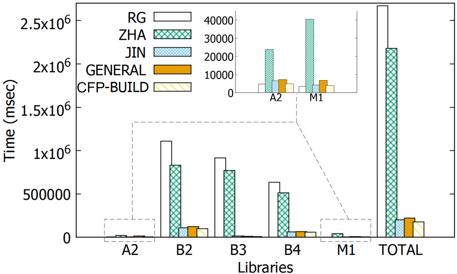
Refer to caption
(a)
Refer to caption
(b)
Figure 10: Efficiency evaluation of proposed TAR derivation algorithms

Furthermore, we observe the acceleration effect of the Algorithm 1 (IMPROVED), which exploits the relations in CFP further than GENERAL (Fig. 10b). We compute the overhead of IMPROVED and GENERAL, i.e., their total TAR derivation time cost minus CFP-BUILD time, which costs the same for both algorithms. In Fig. 10b, the total overheads for GENERAL to derive TAR from CFPs are around 7 times larger than IMPROVED, which indicates that exploiting more CFP relations results in significant acceleration.

6.1.2 Scalability Evaluation

We compare the scalability of GENERAL, IMPROVED with existing JIN, ZHA and RG on artificial Petri nets with growing concurrency structures. In Test A, each net is a single parallel structure with exactly one transition on each branch, and we observe how the increase in the number of concurrent branches affects TAR derivation time. In Test B, we generate concurrent branches of a fixed number (i.e. 5) and observe the effect of the number of transitions on each branch on the performance of algorithms.
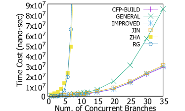
Refer to caption
(a)
Refer to caption
(b)
Figure 11: Scalability evaluation of TAR derivation algorithms

In both tests, CFP-based algorithms (GENERAL, IMPROVED, JIN) scale much better than RG-based algorithms (RG, ZHA). But JIN does not support non-free-choice nets or pTAR whereas GENERAL and IMPROVED do. Among CFP-based algorithms, IMPROVED scales the best with the growing size of concurrency structures, which is more efficient than GENERAL in both tests and has comparable or even better performance than JIN.

6.2 pTAR Computing Performance

To meet their needs for analysis, users may treat various sets of transitions as ‘projected’ transitions (and the rest silent transitions). Therefore, the percentage of silent transitions may differ among scenarios. To observe the performance of pTAR derivation algorithms under this diversity, we run our algorithms on data-sets with different percentages of silent tasks. These data-sets are prepared by marking the same IBM industrial process data-set [20] with varying percentages of silent transitions. We prepare data-sets with five levels of silent task percentage, namely, 10, 30, 50, 70 and 90 percent. Fig. 12a shows the total time cost to derive pTAR from these data-sets under varying percentages of silent transitions, using the three algorithms we have discussed. In the next figures, RG stands for the original reachability-graph-based pTAR computation algorithm [2], CU and RCU denote our algorithm based on locally continued unfolding and its accelerated version using redirected CFP. Fig. 12b,  12c and  12d shows the detailed time cost spent on each library by the three algorithms respectively.
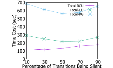
Refer to caption
(a)
Refer to caption
(b)
Refer to caption
(c)
Refer to caption
(d)
Figure 12: pTAR time cost under varying percentage of silent transitions

As can be observed in the above figures, RCU performs the best among all three algorithms we have tested (RG, CU and its accelerated version RCU). Moreover, we could see that by using the redirected CFP and avoid unnecessary local silent extensions, the time cost of RCU is significantly less than CU.

7 Combining TAR and BP for Similarity-based Process Model Querying

The implications of the above results are not only about the improved efficiency of TAR computation. As Behavior Profiles (BP) are also efficiently computable through Petri net unfolding [4], we can easily enhance BP information with additional TAR information by re-using the information contained in the unfolding structure (and vice versa). Therefore, the long-expected combined usage of TAR and BP for process model similarity estimation [6] could now be realized with low overhead because of the above efficient algorithms.

In Sect. 1, we have demonstrated the advantage of TAR over BP in terms of the discriminative power for various process model behaviors (i.e. loops, parallel branches and silent transitions). In this section, we will conduct experiments using industrial benchmark datasets to further illustrate the implications of our proposal for process model similarity estimation.

Our evaluation is based on the scenario of process model retrieval. The problem of process model retrieval is defined as: given some query process model p𝑝p and a repository of process models 𝒞𝒞\mathcal{C}, find in 𝒞𝒞\mathcal{C} process models that are most similar with p𝑝p, and rank them in order of similarity. For benchmark dataset, we used the SAP reference model repository as in [5], which contains 100 process models in total, among which there are 10 query models. The dataset comes with ground-truth tags provided by experts, suggesting which models are similar to which query models by boolean values. For the similarity estimation between tasks with different activity descriptions, we used the label edit distance threshold as in [5] to determine whether two tasks with different descriptions points to the same activity.

For similarity estimation, we use the classic definition of Jaccard coefficient, by which similarity from the perspective of TAR and BP can be given respectively as follows.

Definition 7.1 (TAR Similarity)

For net system N1=(P1,T1,F1)subscript𝑁1subscript𝑃1subscript𝑇1subscript𝐹1N_{1}=(P_{1},T_{1},F_{1}) and N2=(P2,T2,F2)subscript𝑁2subscript𝑃2subscript𝑇2subscript𝐹2N_{2}=(P_{2},T_{2},F_{2}) (with initial markings of M1,M2subscript𝑀1subscript𝑀2M_{1},M_{2} respectively), let TS1𝑇subscript𝑆1TS_{1} and TS2𝑇subscript𝑆2TS_{2} be the TAR set of the two nets, then the TAR similarity between N1subscript𝑁1N_{1} and N2subscript𝑁2N_{2} can be given as follows:

simT((N1,M1),(N2,M2))=|TS1TS2||TS1TS2|𝑠𝑖subscript𝑚𝑇subscript𝑁1subscript𝑀1subscript𝑁2subscript𝑀2𝑇subscript𝑆1𝑇subscript𝑆2𝑇subscript𝑆1𝑇subscript𝑆2sim_{T}((N_{1},M_{1}),(N_{2},M_{2}))=\frac{|TS_{1}\cap TS_{2}|}{|TS_{1}\cup TS_{2}|}
Definition 7.2 (BP Similarity)

For net system N1=(P1,T1,F1)subscript𝑁1subscript𝑃1subscript𝑇1subscript𝐹1N_{1}=(P_{1},T_{1},F_{1}) and N2=(P2,T2,F2)subscript𝑁2subscript𝑃2subscript𝑇2subscript𝐹2N_{2}=(P_{2},T_{2},F_{2})(with initial markings of M1,M2subscript𝑀1subscript𝑀2M_{1},M_{2} respectively), 1subscript1\mathcal{B}_{1} and 2subscript2\mathcal{B}_{2} be the BP set of the two nets, then the BP similarity between N1subscript𝑁1N_{1} and N2subscript𝑁2N_{2} can be given as follows:

simBP((N1,M1),(N2,M2))=|12||12|𝑠𝑖subscript𝑚𝐵𝑃subscript𝑁1subscript𝑀1subscript𝑁2subscript𝑀2subscript1subscript2subscript1subscript2sim_{BP}((N_{1},M_{1}),(N_{2},M_{2}))=\frac{|\mathcal{B}_{1}\cap\mathcal{B}_{2}|}{|\mathcal{B}_{1}\cup\mathcal{B}_{2}|}

Consequently, the ranking functions for process models in C𝐶C given a query model pP𝑝𝑃p\in P can be given as follows

Definition 7.3 (TAR Ranking)

For some query model ppPsubscript𝑝𝑝𝑃p_{p}\in P and some target model pcsubscript𝑝𝑐p_{c} in repository C𝐶C, the TAR ranking of pcsubscript𝑝𝑐p_{c} is given as

RT(pp,pc)=|{pcC|simT(pp,pc)simT(pp,pc)}|subscript𝑅𝑇subscript𝑝𝑝subscript𝑝𝑐conditional-setsuperscriptsubscript𝑝𝑐𝐶𝑠𝑖subscript𝑚𝑇subscript𝑝𝑝subscriptsuperscript𝑝𝑐𝑠𝑖subscript𝑚𝑇subscript𝑝𝑝subscript𝑝𝑐R_{T}(p_{p},p_{c})=|\{p_{c}^{\prime}\in C|sim_{T}(p_{p},p^{\prime}_{c})\geq sim_{T}(p_{p},p_{c})\}|
Definition 7.4 (BP Ranking)

Similarly, for some query model ppPsubscript𝑝𝑝𝑃p_{p}\in P and some target model pcsubscript𝑝𝑐p_{c} in repository C𝐶C, the BP ranking of pcsubscript𝑝𝑐p_{c} is given as

RBP(pp,pc)=|{pcC|simBP(pp,pc)simBP(pp,pc)}|subscript𝑅𝐵𝑃subscript𝑝𝑝subscript𝑝𝑐conditional-setsuperscriptsubscript𝑝𝑐𝐶𝑠𝑖subscript𝑚𝐵𝑃subscript𝑝𝑝subscriptsuperscript𝑝𝑐𝑠𝑖subscript𝑚𝐵𝑃subscript𝑝𝑝subscript𝑝𝑐R_{BP}(p_{p},p_{c})=|\{p_{c}^{\prime}\in C|sim_{BP}(p_{p},p^{\prime}_{c})\geq sim_{BP}(p_{p},p_{c})\}|

We may use the product of TAR ranking and BP ranking to combine their influence to the similarity ranking result as follows:

Definition 7.5 (TAR-BP Ranking)

For some query model ppPsubscript𝑝𝑝𝑃p_{p}\in P and some target model in pcCsubscript𝑝𝑐𝐶p_{c}\in C, the TAR-BP ranking of pcsubscript𝑝𝑐p_{c} can be given as

RTBP(pp,pc)=|{pcC|RT(pp,pc)RBP(pp,pc)R_{TBP}(p_{p},p_{c})=|\{p_{c}^{\prime}\in C|R_{T}(p_{p},p^{\prime}_{c})\cdot R_{BP}(p_{p},p^{\prime}_{c})\leq
RT(pp,pc)RBP(pp,pc)}|R_{T}(p_{p},p_{c})\cdot R_{BP}(p_{p},p_{c})\}|

With the above similarity ranking functions, we evaluate the process model retrieval performance when (1) only TAR (2) only BP and (2) both TAR and BP are considered. In Fig. 13 we compared the precision-recall performance of these three cases. It can be observed that the combined usage of TAR and BP could improve the overall performance of process model retrieval, which agrees with our previous discussions in Sect. 1.
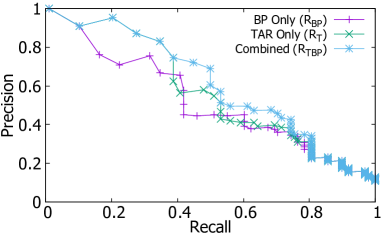
Refer to caption
Figure 13: Recall-precision performance of different similarity measures

8 Conclusion

In this article we proposed comprehensive strategies for the computation of TAR and pTAR based on Petri net unfoldings. These strategies attempt to exploit as much information in unfoldings as possible, by translating causal patterns and co𝑐𝑜co-relation patterns into TAR/pTAR results. The fundamental challenge of unfolding based TAR/pTAR computation is the handling of cut-off events, which may truncate information needed for TAR/pTAR confirmation. Novel techniques to derive locally continued unfolding and redirected CFP for efficient recovery of necessary information after cut-off events are proposed, proved and evaluated in this article. Experiments show that the proposed strategies achieve significant performance improvement over existing methods based on reachability graphs. This will support further researches and more scalable applications of TAR/pTAR in various business process analytic tasks.

References

  • [1] H. Zha, J. Wang, L. Wen, C. Wang, and J. Sun. “A workflow net similarity measure based on transition adjacency relations,” Computers in Industry, vol. 61, no.5, pp. 463–471, 2010.
  • [2] J. Prescher, J. Mendling, and M. Weidlich. “The Projected TAR and its Application to Conformance Checking,” in Proceedings of the 5th International Workshop on Enterprise Modelling and Information Systems Architectures (EMISA), 2012, pp. 151–164.
  • [3] M. Weidlich, J. Mendling, and M. Weske. “Efficient consistency measurement based on behavioral profiles of process models,” IEEE Transactions on Software Engineering, vol. 37, no. 3, pp. 410–429, 2011.
  • [4] M. Weidlich, F. Elliger, and M. Weske. “Generalised computation of behavioural profiles based on petri-net unfoldings,” in Proceedings of the 7th International Workshop on Web Services and Formal Methods (WS-FM), 2010, pp. 101–115.
  • [5] R. Dijkman, M. Dumas, B. F. van Dongen, R. Käärik, and J. Mendling. “Similarity of business process models: Metrics and evaluation,” Information Systems, vol. 36, no. 2, pp. 498–516, 2011.
  • [6] M. Becker, and R. Laue. ”A comparative survey of business process similarity measures,” Computers in Industry, vol. 63, no. 2, pp. 148–167, 2012.
  • [7] M. Dumas, L. Garcia-Banuelos, and R. Dijkman. “Similarity Search of Business Process Models,” IEEE Data Engineering Bulletin, vol. 32, no. 3, pp. 23–28, 2009.
  • [8] T. Jin, J. Wang, and L. Wen. “Efficient retrieval of similar workflow models based on behavior,” in Proceedings of the 14th Asia-Pacific Web Conference (APWeb), 2012, pp. 677–684.
  • [9] L. Wen, J. Wang, W. M. P. van der Aalst, B. Huang, and J. Sun. “Mining process models with prime invisible tasks,” Data & Knowledge Engineering, vol. 69, no. 10, pp. 999–1021, 2010.
  • [10] W. M. P.  van der Aalst. Process Mining: Data Science in Action. Springer, 2016.
  • [11] A. Rozinat, and W. M. P. van der Aalst. “Conformance checking of processes based on monitoring real behavior,” Information Systems, vol. 33, no. 1, pp. 64–95, 2008.
  • [12] W. M. P. van der Aalst, and T. Basten. “Inheritance of workflows: an approach to tackling problems related to change,” Theoretical Computer Science, vol. 270, no. 1–2, pp. 125–203, 2002.
  • [13] A. Polyvyanyy, M. Weidlich, R. Conforti, M. La Rosa, A. H. M. ter Hofstede. “The 4C Spectrum of Fundamental Behavioral Relations for Concurrent Systems,” in Proceedings of the 35th International Conference on Applications and Theory of Petri Nets and Concurrency (Petri Nets), 2014, pp. 210–232.
  • [14] J. Esparza, and C. Schroeter. “Unfolding Based Algorithms for the Reachability Problem,” Fundamenta Informaticae, vol. 47, no. 3–4, pp. 231–245, 2001.
  • [15] J. Pei, L. Wen, X. Ye, A. Kumar, and Z. Lin. “Transition Adjacency Relation Computation Based on Unfolding: Potentials and Challenges,” in Proceedings of the Confederated International Conferences: CoopIS, C&TC, and ODBASE (OTM), 2016, pp. 61–79.
  • [16] T. Murata. “Petri nets: Properties, analysis and applications,” Proceedings of the IEEE, vol. 77, no. 4, pp. 541–580, 1989.
  • [17] J. Esparza, S. Romer, and W. Vogler. “An improvement of McMillan’s unfolding algorithm,” Formal Methods in System Design, vol. 20, no. 3, pp. 285–310, 2002.
  • [18] K. L. McMillan, and D. K. Probst. ”A technique of state space search based on unfolding,” Formal Methods in System Design, vol. 6, no. 1, pp. 45–65, 1995.
  • [19] J. Pei, L. Wen, X. Ye. “Computation of Transition Adjacency Relations Based on Complete Prefix Unfolding (Technical Report),” arXiv:1512.00428v3, 2017.
  • [20] D. Fahland, C. Favre, B. Jobstmann, J. Koehler, N. Lohmann, H. Völzer, and K. Wolf. “Instantaneous soundness checking of industrial business process models,” in Proceedings of the 7th International Conference on Business Process Management (BPM), 2009, pp. 278–293.
[Uncaptioned image] Jisheng Pei received his BS degree in Computer Software and his PhD degree in Computer Science from Tsinghua University. His research interests include the processing and analysis methods of data provenance, process mining, similarity measurements of process traces and models, as well as behavior analytics and service computing.
[Uncaptioned image] Lijie Wen received the BS degree, the Ph.D. degree in Computer Science and Technology from Tsinghua University, Beijing, China, in 2000 and 2007 respectively. He is currently an associate professor at School of Software, Tsinghua University. His research interests are focused on process mining, process data management (e.g., log completeness, trace clustering, process similarity, process indexing and retrieval), and lifecycle management of workflow for big data analysis.
[Uncaptioned image] Xiaojun Ye received the BS degree in mechanical engineering from Northwest Polytechnical University, Xian, China, in 1987 and the Ph.D. degree in information engineering from INSA Lyon, France, in 1994. Currently, he is a professor at School of Software, Tsinghua University, Beijing, China. His research interests include cloud data management, data security and privacy, and database system testing.
[Uncaptioned image] Akhil Kumar has a PhD from the University of California, Berkeley, and is a full professor of information systems at the Smeal College of Business, Pennsylvania State University. His current research interests are in business process management (BPM) and workflow systems, process mining, supply chain and business analytics, and health IT. He is a senior member of IEEE and an associate editor for ACM Transactions on Management Information System. He served as a co-chair for the International Business Process Management Conference in 2017. He has been a principal investigator for National Science Foundation and also received support from IBM, HP, and other organizations for his work.