Deuteration in infrared dark clouds

Abstract

Much of the dense gas in molecular clouds has a filamentary structure but the detailed structure and evolution of this gas is poorly known. We have observed 54 cores in infrared dark clouds (IRDCs) using N₂H⁺ (1–0) and (3–2) to determine the kinematics of the densest material, where stars will form. We also observed N₂D⁺ (3–2) towards 29 of the brightest peaks to analyse the level of deuteration which is an excellent probe of the quiescent of the early stages of star formation. There were 13 detections of N₂D⁺ (3–2). This is one of the largest samples of IRDCs yet observed in these species. The deuteration ratio in these sources ranges between 0.003 and 0.14. For most of the sources the material traced by N₂D⁺ and N₂H⁺ (3–2) still has significant turbulent motions, however three objects show subthermal N₂D⁺ velocity dispersion. Surprisingly the presence or absence of an embedded 70$\upmu$m source shows no correlation with the detection of N₂D⁺ (3–2), nor does it correlate with any change in velocity dispersion or excitation temperature. Comparison with recent models of deuteration suggest evolutionary time-scales of these regions of several freefall times or less.

1 Introduction

Through their radiative, kinetic and chemical feedback into the interstellar medium, massive stars play a dominant role in the shaping and evolution of galaxies. However, the formation process and early evolution of high-mass stars is not well understood. Several factors contribute to this: (1) high-mass stars are intrinsically much rarer than their low-mass counterparts implying that they are generally observed at larger distances; (2) high-mass stars are rarely (if ever) formed in isolation, but in the complex environment of clusters and (3) high-mass stars, and in particular their youngest phases, are short lived. In addition, once formed, the feedback from young massive stars rapidly reshapes the regions in which they form. Young massive stars are therefore typically seen in a complex environment involving gravitational interaction, winds, outflows and ionizing radiation. Thus the study of high-mass star from both observational and theoretical point of view is much more complex than that of low-mass star formation, with little consensus on the key mechanisms (Zinnecker & Yorke 2007). To make progress it is crucial to identify massive star formation regions in their earliest stages, when the initial conditions and first stages of evolution can be studied. Capturing these rare phases requires a large initial sample of massive, quiescent regions which could, or are just starting to, form massive stars.

Infrared dark clouds (IRDCs) are defined as regions with significant extinctions viewed against the bright, diffuse mid-infrared galactic background. Such regions were first detected by the Infrared Space Observatory (ISO) and then by the Midcourse Space Experiment (MSX; Perault et al. 1996; Egan et al. 1998; Hennebelle et al. 2001), and are ubiquitous throughout the Galaxy (Simon et al. 2006). Previous studies show that their molecular material has low temperatures ($<$25 K), high column densities ($\sim 10^{23}--10^{25}$ cm^-2), and high-volume densities ($>$10⁵ cm^-3; Egan et al. 1998, Carey et al. 1998, 2000, Peretto & Fuller 2009, 2010). IRDCs have been described as possible precursors to the initial stages of massive star formation (Rathborne et al. 2006). Studies have shown (e.g. Teyssier et al. 2002; Pillai et al. 2006; Rathborne et al. 2006) that IRDCs are cold, and contain dense structures with sizes and masses comparable to warmer cluster-forming clumps and as well as compact cores with sizes, masses, and densities comparable to high-mass star-forming hot cores. Thus, IRDCs are a great starting place to search for the most quiescent and earlier stages of massive star formation.

Deuterium-containing molecular species allow us to study the quiescent and cold material in a molecular cloud. The deuterated species preferentially trace the coldest parts of dense cores (i.e. single star progenitors), and have been shown to be an important tool to determine the degree of evolution in low-mass cores (Caselli et al. 2002; Crapsi et al. 2005; Emprechtinger et al. 2009) and high-mass cores (Fontani et al. 2011; Pillai et al. 2012). Chemical models (e.g. Kong et al. 2015) show increased deuterium enhancement with time in these cold and dense regions. In the prestellar core phase, the deuteration fractionation increases and CO freezes out on to grains as the core contracts, reaching maximum when star formation begins. In the prestellar phase the C-bearing species are therefore depleted towards the densest regions, while N-bearing species are good tracers of the total column density even at high volume densities. After the formation of a protostar, the deuteration fraction decreases as the protostar evolves, heats its environment and the CO is released from the dust grains. So a high deuteration fraction in a protostellar core indicates the youth of the protostar, while a high deuteration fraction in a pre-stellar core indicates that the core may soon collapse into a protostar. Thus, the deuteration ratio is an excellent probe of the early stages of star formation (e.g. Pineda & Teixeira 2013). A systematic study of deuteration towards high-mass star-forming regions will likely unveil a range of objects in different evolutionary stages, and will pinpoint the most likely candidates for the most quiescent regions.

In this paper, we use N₂H⁺ and its deuterated counterpart N₂D⁺ to study over 50 targets which are thought to be regions of massive star formation. In Section 2 of this paper, we present the source selection, data, and data reduction used in this study. Section 3 presents the analysis of the reduced data, and we show the derived parameters such as the excitation temperature and velocity dispersion. In Section 4, we present the results: the presence of multiple components, the derived deuteration ratios, and the turbulence on small scales. In Section 5, we discuss and analyse the results: showing the effects of the filling factor on the deuteration ratio, the presence and influence of a 70 $\upmu$m source in the region, and we provide an estimate to the age of the regions. Finally in Section 6, we summarize our results.

2 Data

2.1 Catalogue and initial MOPRA observations

The Spitzer Dark Cloud (SDC) catalogue is a survey and analysis of IRDCs in the Galaxy using the Spitzer GLIMPSE 8$\upmu$m data (Peretto & Fuller, 2009). More than 11000 sources are identified in $10\degr<|l|<65\degr$ and $0\degr<|b|<1\degr$. From this catalogue we picked individual IRDCs or IRDCs-complexes to analyse the dense gas distribution and properties. Individual IRDCs were selected because they have a filamentary shape. The IRDCs-complexes were selected because of their filamentary shape in a larger scale.

Using the Australia Telescope National Facility (ATNF) MOPRA 22m telescope we observed molecular lines at 3mm, including the HNC (1–0) and N₂H⁺ (1–0) lines, towards these objects. The observations were carried out in 2010 May, 2011 July and 2012 July. The data was reduced using gridzilla . The MOPRA beam FWHM is 36 arcsec at the observed wavelength. The noise rms range was 60–330 mK after smoothing the spectra to a 0.22 km s^-1 channel spacing. One long IRDCs-complex was mapped, and eight individual IRDCs were mapped. Additionally 66 single pointings were made towards the densest parts of 14 IRDCs. The large IRDC complex, which we call L332, is a $\sim 0.5\degr$ long which encompasses more than 36 individual IRDCs. The HNC and N₂H⁺ (1–0) maps exhibits a coherent structure connecting all the single IRDCs (Lackington et al., in preparation).

The N₂H⁺ (1–0) spectra were reduced using the procedure described in Section 3, and the results of fitting the hyperfine structure are shown in Table 3.

2.2 APEX

From the MOPRA maps and single-pointing spectra we selected the brightest cores in these IRDCs. Since the HNC(1–0) and N₂H⁺ (1–0) peaks are well correlated (Lackington et al., in preparation) and HNC has higher signal to noise we used the peaks identified by the HNC (1–0) emission. Fig. 1 shows how these positions were selected in the L332 IRDC-complex. Using the Atacama Pathfinder EXperiment (APEX) telescope we observed N₂H⁺ (3–2) and N₂D⁺ (3–2) towards the selected cores. For the selected lines the APEX beam is smaller (22–27 arcsec) than the MOPRA beam (Fig. 1), meaning we are probing smaller scales. The observations of N₂H⁺ and N₂D⁺ (3–2) were carried out in 2012 August–November with APEX. In total 54 N₂H⁺ (3–2) single-pointing observations (Table 1), using the APEX-2 receiver of the Swedish Heterodyne Facility Instrument (SHeFi; Vassilev et al. 2008), were made. The cores with the brightest and narrowest N₂H⁺ (3–2) line were also observed in N₂D⁺ (3–2) using the APEX-1 receiver of the SHeFi. In total 29 cores were observed in N₂D⁺ (3–2). That makes this list the largest sample of deuterium observations towards high-mass star-forming regions. The positions observed in N₂H⁺ and N₂D⁺ (3–2) are listed in Table 2. Instead of using individual IRDCs names to identify the positions observed in the L332 complex we numbered the 15 peaks observed in the region, and we use this as the identifier.

Table 1: Summary of observations for observed transitions.

Transition	Objects observed	Objects detected
N2H+ (3–2)	53	53
N2H+ (3–2)	54	51
N2D+ (3–2)	29	13

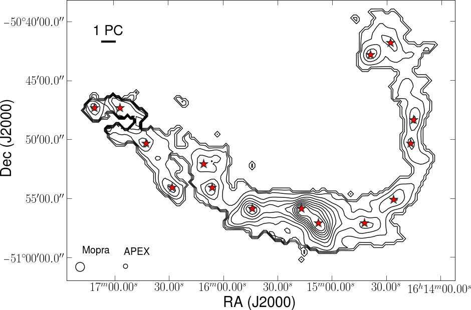
Figure 1: MOPRA HNC (1–0) velocity integrated intensity map towards the filamentary complex of IRDCs, L332. Contours represent 90, 80,. . ., 20, 10, 5 per cent of the peak value. The red stars represent the selected positions to observe N₂H⁺ and N₂D⁺ (3–2) using APEX. In lower-left, we show the MOPRA and APEX beams for comparison.

The observations used position switching, and were calibrated by regularly measuring the sky brightness and cold/hot loads in the cabin. All observations used the extended bandwidth Fast Fourier Transform Spectrometer (XFFTS), which provides two 2.5 GHz units, with 32 768 channels each unit and 1 GHz overlap. This configuration provides an spectral resolution of 0.082 and 0.099 km s^-1 for N₂H⁺ (3–2) and N₂D⁺ (3–2), respectively. The N₂H⁺ (3–2) observations had a T_sys range of 117–150 K, and noise rms range of 58–400 mK. For the N₂D⁺ (3–2) observations the T_sys range was 145–158 K, and the noise rms range was 24–67 mK after smoothing the spectra to a 0.197 km s^-1 channel spacing. The APEX half power beam width (HPBW) for N₂H⁺ (3–2) is 22 arcsec, which at a typical distance for the sample of 3.1 kpc (see Section 4.3) corresponds to a typical size of 0.33 pc. On the other hand the APEX HPBW for N₂D⁺ (3–2) is 27 arcsec which means a size of 0.4 pc at 3.1 kpc.

All spectra were reduced using class90. Before averaging all the scans, each spectrum had the baseline removed by fitting a first- or second-order polynomial.

Table 2: Observed positions. The columns show the source name, right ascension (J2000), declination (J2000), and number of young stellar objects (YSO) within the APEX beam for N₂D⁺ (3–2).

Source	RA (J2000)	Dec. (J2000)	YSOs in beam
SDC299.2	12:18:26.289	-63:01:31.710	0
SDC320.271	15:07:56.547	-57:54:16.420	1
SDC320.252	15:07:21.101	-57:49:14.420	1
SDC321.708	15:18:01.201	-57:21:55.150	1
SDC321.758	15:18:26.711	-57:21:44.740	0
SDC321.936	15:19:42.442	-57:17:50.750	0
SDC329.028	16:00:30.790	-53:12:29.200	1
SDC329.068	16:01:08.860	-53:15:38.500	0
SDC329.186	16:01:46.800	-53:11:45.000	1
SDC329.313	16:02:23.440	-53:05:59.700	1
SDC351.438	17:20:53.900	-35:45:21.000	0
SDC352.027	17:22:33.937	-35:13:11.220	0
SDC351.8	17:21:49.399	-35:27:31.150	0
SDC351.562	17:20:52.217	-35:35:09.840	0
L332-10	16:14:42.115	-50:57:07.776	0
L332-11	16:14:26.280	-50:55:07.356	0
L332-12	16:14:16.874	-50:50:22.056	0
L332-13	16:14:15.336	-50:48:21.996	0
L332-14	16:14:28.121	-50:41:52.404	0
L332-15	16:14:39.156	-50:42:52.704	0
L332-1	16:17:10.946	-50:47:20.004	0
L332-3	16:16:42.559	-50:50:21.444	1
L332-4	16:16:28.397	-50:54:06.984	1
L332-5	16:16:10.920	-50:52:07.536	0
L332-6	16:16:06.197	-50:54:07.668	0
L332-7	16:15:44.011	-50:55:53.040	1
L332-8	16:15:17.038	-50:55:53.184	1
L332-9	16:15:07.512	-50:57:08.136	0
SDC335.283A	16:29:01.428	-48:50:28.464	1
SDC335.283B	16:28:50.800	-48:50:42.300	0
SDC335.077A	16:29:22.270	-49:12:14.616	0
SDC335.077B	16:29:28.900	-49:10:54.500	0
SDC335.579A	16:31:01.900	-48:44:04.000	0
SDC335.579B	16:30:54.800	-48:42:43.000	0
SDC335.579Y1	16:30:58.800	-48:43:54.000	1
SDC335.579Y2	16:30:57.300	-48:43:40.000	1
SDC335.44	16:30:03.900	-48:48:38.000	0
SDC335.253	16:29:42.900	-48:58:48.000	0
SDC335.229A	16:29:35.800	-48:59:48.000	0
SDC335.229B	16:29:38.800	-49:00:40.000	0
SDC335.059	16:29:11.700	-49:11:36.000	0
SDC356.84	17:37:57.149	-31:36:13.176	0
SDC13.174A	18:14:30.413	-17:33:08.712	1
SDC13.174B	18:14:26.220	-17:31:53.688	0
SDC13.194	18:14:33.559	-17:31:08.688	0
SDC16.915	18:21:55.877	-14:15:03.672	1
SDC2.141	17:49:32.652	-26:57:07.812	0
SDC2.116	17:49:24.283	-26:58:24.060	0
SDC301.876	12:42:19.298	-62:14:40.200	1
SDC327.894	15:51:52.740	-53:26:11.688	1
SDC327.964	15:52:31.486	-53:26:50.388	0
SDC34.558	18:52:34.358	+01:41:11.580	0
SDC37.08	18:59:04.134	+03:38:31.670	1

3 Analysis

The N₂H⁺ (1–0), N₂H⁺ (3–2) and N₂D⁺ (3–2) transitions have hyperfine structure, which allows independent calculation of the optical depth, $\tau_{0}$, and the excitation temperature, $T_{\text{ex}}$. The lines were fitted in python using the Levenberg–Marquardt least-squares minimization routine mpfit. The model we used takes into account all the hyperfine components, and depends on four variables: optical depth ($\tau_{0}$), excitation temperature ($T_{\text{ex}}$), central velocity ($v_{\text{c}}$), velocity dispersion ($\sigma$; also described as the linewidth hereafter). The approach we use is similar to the one by Fuller & Myers (1993), Rosolowsky et al. (2008) and Pineda & Teixeira (2013). The expected emission is,

$$T_{\text{mb}}(\nu)=A[1-e^{-\tau(\nu)}],$$ (1)

where T${}_{\text{mb}}$ is the main beam temperature, which was obtained using the telescope efficiency, 0.74 for N₂H⁺ (3–2), and 0.75 for N₂D⁺ (3–2). Also

$$\tau(\nu)=\tau_{0}\,\sum_{i=1}^{N}a_{i}\,e^{-[(v-v_{\text{c}})\,+\,v_{i}]^{2}/2\sigma^{2}},$$ (2)

$$\sum_{i=1}^{N}a_{i}=1,$$ (3)

$$A=\eta_{\text{f}}[J(T_{\text{ex}})-J(T_{\text{bg}})],$$ (4)

and,

$$J(T)={h\nu\over k}{1\over\exp(h\nu/kT)-1},$$ (5)

where $v_{i}$ is the velocity offset of the ith hyperfine component, and $a_{i}$ is its statistical weight, and $\eta_{\text{f}}$ is the beam filling factor.

N₂H⁺ (3–2) has 45 hyperfine components, and N₂D⁺ (3–2) has 25 hyperfine components. The rest frequencies used were 231.3219 and 279.5118 GHz for N₂D⁺ (3–2) and N₂H⁺ (3–2) respectively. Due to the linewidths of our sample the N₂H⁺ (3–2) hyperfine components are blended and exhibit at most three blended components. On the other hand the linewidths and noise of N₂D⁺ (3–2) observations blend its hyperfine components into only one peak feature above the noise level.

Since the spatial extent of the emission is unknown we assume $\eta_{\text{f}}=1,$ which provides us with a lower limit to the true column densities. With this assumption $T_{\text{ex}}$ is obtained from the fit when $\tau_{0}$ is well constrained. In addition, $\tau_{0}$ is limited in the 0.1–30 range as outside this limits the equation becomes degenerate. In the optically thick limit exp($-\tau_{0})\ll$ 1, and in the optically thin limit 1 – exp($-\tau_{0})\approx\tau_{0}$ making $\tau_{0}$ and $T_{\text{ex}}$ degenerate. To avoid the optically thin degeneracy if $\tau_{0}\leq 0.1$, and thus $T_{\text{ex}}$ is not constrained, we assumed $\tau_{0}=0.1$. Using this criteria, three sources are optically thin.

Example spectra N₂H⁺ (3–2) and N₂D⁺ (3–2) are shown in Figure 2. Both lines towards this object are well fitted using a single velocity component which is shown in the figure. Similar figures for all the sources are shown in the appendix which is available online.

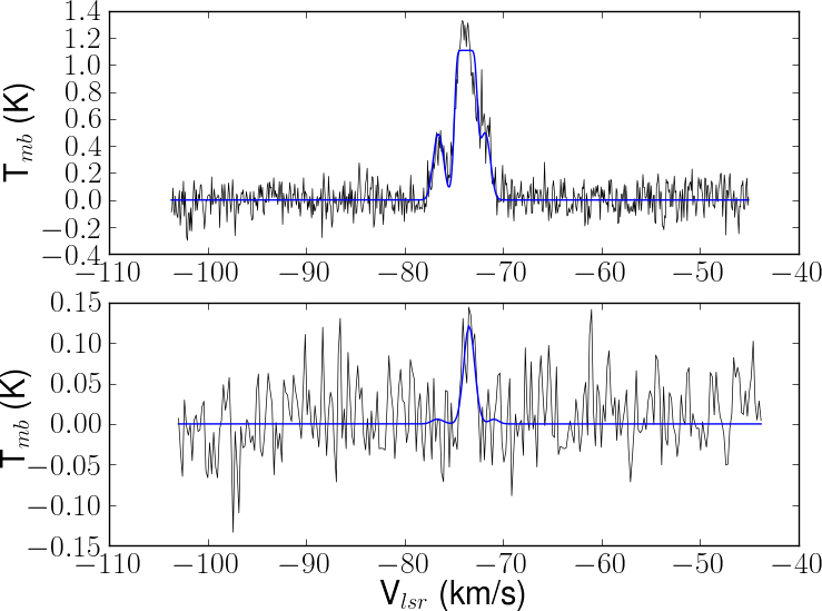
Figure 2: SDC329.313 spectra: N₂H⁺ (3–2) (top) and N₂D⁺ (3–2) (bottom) sample spectra overplotted with the hyperfine component model fit.

3.1 Distances

Distances to the clouds were computed using an adaptation to python from the idl routine ’kindist.pro’, which uses a galactic rotation curve to calculate kinematic distances. The constants used are 8.4 kpc of galactocentric distance and local standard of rest (LSR) velocity of 254 km s^-1 around the galactic centre (Reid et al. 2009). For all sources except for the group around of four pointings around SDC351.8 we obtained reasonable values. The calculated values for these sources varied from 250pc to 1kpc, a spread unlikely given that they are from the same region and have similar velocities. In addition, 250 pc is very small compared to the rest of the sample which also seems unlikely. So for this source we will use the mean distance of the sample, 3.1 kpc. For SDC299.2 and SDC301.876 the measured central velocity was beyond the tangent point value, so again we used the mean distance.

4 Results

The N₂H⁺ (3–2) spectra have typical noise levels of 0.124 K in the 0.08 km s^-1 velocity channels while the N₂D⁺ (3–2) spectra has typical noise levels of 0.04 K in 0.2 km s^-1 velocity channels. Meanwhile the N₂H⁺ (1–0) spectra have typical noise levels of 0.11 K after smoothing the spectra to a 0.22 km s^-1 velocity channels. We detected N₂H⁺ (3–2) emission towards 51 of the 54 pointings. Only SDC13.174B, SDC335.253, and SDC335.077B did not exhibit N₂H⁺ (3–2) emission. N₂D⁺ (3–2) emission was detected towards 13 of the 29 pointings (Table 1). Finally N₂H⁺ (1–0) was detected towards 52 of the 53 pointings.

For 38 out of the 51 N₂H⁺ (3–2) observations a good fit is obtained with a single velocity component. Tables 4 and 5 shows the results of the hyperfine structure fitting to the N₂H⁺ (3–2) line of the detected objects. A two-component fit is necessary in 13 cases, which present two distinct components along the line of sight or line asymmetry consistent with an additional component along the line of sight. In these cases two independent velocity components are fitted simultaneously, with each component labelled ‘-a’ or ‘-b’. The fitted parameters for the two velocity components are shown in Tables 4 and 5. On the other hand all the N₂H⁺ (1–0) detections are well fitted with only one velocity component.

For N₂H⁺ (3–2) the fitting procedure gives well-constrained parameters for all except 15 sources. These 15 sources had poorly constrained optical depth ($\tau_{0}<3\sigma_{\tau}$, where $\sigma_{\tau}$ is the estimated uncertainty in the optical depth). For these sources we fix the excitation temperature to the average value obtained from all other spectra, i.e., 6.5 K. This removes one free parameter in the fit providing better constrained estimates of the other parameters.

Due to the low signal to noise and blending of the hyperfine components of the N₂D⁺ (3–2), the full four-parameter fit gives badly constrained parameters. Since both transitions have similar critical densities, we fix the N₂D⁺ (3–2) excitation temperature to the value from the N₂H⁺ (3–2) fit. This procedure is similar to the one followed by Crapsi et al. (2005) and Pineda & Teixeira (2013). For N₂D⁺ (3–2), in all cases the optical depth obtained from the hyperfine structure fit is lower than 1. Therefore, we assume that N₂D⁺ (3–2) emission is optically thin in the further analysis. Table 6 shows the results of the hyperfine structure fitting to the N₂D⁺ (3–2) line.

N₂D⁺ (3–2) was detected towards 13 of the 29 pointings. The detections may be because there is something inherently different in these objects. To evaluate this possibility we separated the two samples, detections and non-detections of N₂D⁺ (3–2), and performed statistical tests on the derived properties. We use the Kolmogorov–Smirnov test to determine if the derived properties of both samples follow the same distribution, and Student’s t-tests to evaluate if the samples means are statistically different. We compare the detected and non-detected samples on the N₂H⁺ (3–2) velocity dispersion, integrated intensity, column density, optical depth, and excitation temperature.

The tests show no significant difference between the detected and non-detected objects except in the excitation temperature, $T_{\text{ex}}$. For all the other properties we can not reject the null hypothesis, of identical distributions, at more than a 0.05 level. The distributions of $T_{\text{ex}}$ for the detected and non-detected sources are shown in Fig. 3. The detected sources have a mean $T_{\text{ex}}$ of 9.0 $\pm$ 0.4, while the non-detections appear cooler with a mean $T_{\text{ex}}$ of 6.2 $\pm$ 0.1, perhaps suggesting a difference in density between the objects. However, whether the non-detections reflect the intrinsic difference in the abundance of N₂D⁺, or the excitation of N₂D⁺ and the detectability of the 3-2 transitions awaits a detailed analysis of the N₂D⁺ excitation in these sources.

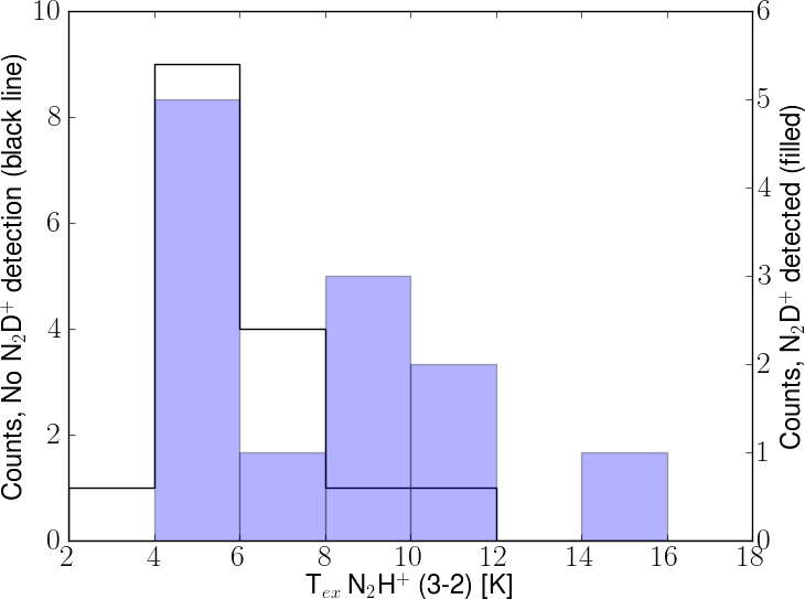
Figure 3: Histogram of N₂H⁺ (3–2) excitation temperature for two subsamples of the sources with observations of N₂H⁺ (3–2): filled is the histogram for sources with detected N₂D⁺ (3–2) (right hand scale), and the black line is the histogram for sources without detection (left-hand scale).

We calculated the column density of N₂H⁺ (1–0), N₂H⁺ (3–2) and N₂D⁺ (3–2) using equations in appendix A of Pineda & Teixeira (2013). For both N₂H⁺ transitions we used the optically thin case if $\tau_{0}<0.1$ or $\tau_{0}<3\sigma_{\tau}$ (three sources). For N₂D⁺ (3–2) we use the optically thin equation. Assuming a filling factor of unity, the derived column densities represent a lower limit of the true values.

The calculated N₂H⁺ column density varies depending on which transition is used. For sources with relatively low (1–0) derived column densities but apparently large ($>$ 5) (3–2) optical depths, the (3–2) derived column densities are much larger (about 10–80 times) than the (1–0) derived column densities. We attribute this to two factors: overestimation of the optical depth of the (3–2) transition (and underestimation of its uncertainties) in part due to the interdependence of the optical depth and velocity dispersion when fitting the lines, and difference in filling factors in both transitions. Because of the possible overestimation of the (3–2) optical depth, the (1–0) derived column densities should be more reliable.

4.1 Line modelling

We attempted to correct the incongruence of the different derived column densities by modelling the N₂H⁺ emission using a non-LTE molecular radiative transfer, radex (van der Tak et al. 2007). For each object we run radex using as inputs: the observed N₂H⁺ (1–0) linewidth, a range of kinetic temperatures (5–20 K), a range of H₂ densities (10⁵–2$\times$10⁶ cm^-3), and a range of N₂H⁺ column densities (0.1–10 times the N₂H⁺ (1–0) derived value). In addition we introduced a filling factor for the (1–0) transition in the analysis of the models.

To discriminate between all the models we used the observed integrated intensity which does not depend on any modelling or line fitting, and the optical depth of the (1–0) which can be obtained with high certainty as it is well constrained by the hyperfine fit. We produced a first cut by selecting the radex-derived models that had an N₂H⁺ (1–0) optical depth equal within 10% of the observed value or within the error in the observation, whichever was greater. From the remaining models we produced a second cut by only keeping only the models with N₂H⁺ (1–0) integrated intensity within 10% of the observed value or within the error in the observation. To do this a beam filling factor was introduced for the models. Finally only the models where the N₂H⁺ (3–2) integrated intensity matched the observation (again within 10% or the observation error) were selected.

The number of objects for which models reproduce the observations varied for each filling factor. The best results were obtained with a filling factor of 0.4 for the N₂H⁺ (1–0) transition, where half of the objects had models (more than for any other filling factor used). Fig. 4 shows an example of how the final radex model fit the observed N₂H⁺ (1–0) and (3–2) lines. Assuming equal sizes of the emission regions for (1–0) and (3–2) transitions, a beam filling factor of 0.4 for the (1–0) emission implies a filling factor of unity for the (3–2) beam. Fig. 5 shows the result of the modelling. The mean value of the N₂H⁺ column density for all the models obtained of each object is plotted versus the N₂H⁺ column density derived from the (1–0) observation using a filling factor of 0.4. It is remarkable that there is a very good agreement between the two values. This is quantified by calculating the linear regression of the values. The obtained slope 1.01 and the r-value is 0.88, meaning that on average the models represent a good fit of the observations.

The kinetic temperatures obtained through the radex modelling range from 5.6 to 19.1 K. The radex obtained densities vary from 2.9 $\times$ 10⁵ to 2 $\times$ 10⁶ cm^-3.

Thus a filling factor of 0.4 is a good approximation for this sample. So for the rest of the paper we use the N₂H⁺ column density derived from the (1–0) observations using a filling factor of 0.4. Table 3 lists this derived value. Tables 4 and 5 list the value of the (3–2) derived N₂H⁺ column density for reference. Finally Table 6 lists the N₂D⁺ column density which assumes a filling factor of unity.

The modelling implies a fractional abundance of N₂H⁺ of 3.6 $\times 10^{-10}$ to 2.6 $\times 10^{-8}$ for the different objects. These values are similar to those observed by other studies. Using MOPRA Miettinen (2014) found fractional abundances of 2.8 $\times 10^{-10}$–9.8 $\times 10^{-9}$ towards IRDCs. Similarly Sanhueza et al. (2012) found abundances of 1.9 $\times 10^{-10}$–1.67 $\times 10^{-8}$.

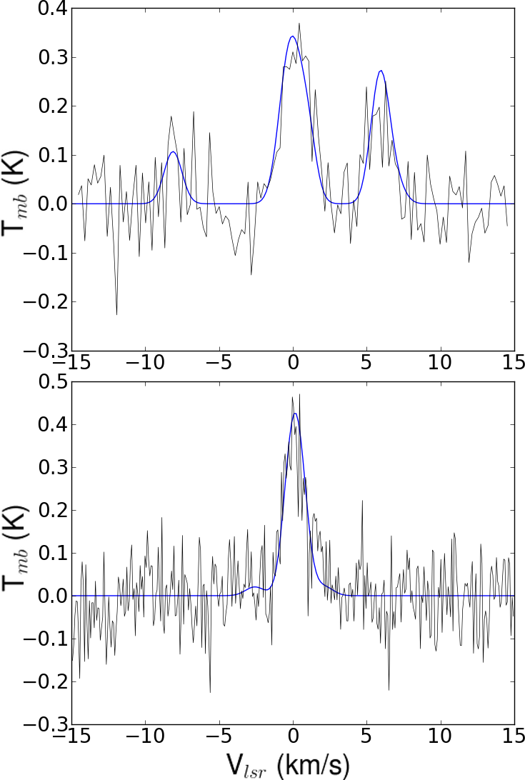
Figure 4: Example of radex derived model for N₂H⁺ towards L332-11. Top: radex model (blue line) over the observed N₂H⁺ (1–0) spectra. Bottom: the same radex model over the observed N₂H⁺ (3–2) spectra. In both cases, the obtained radex model fits the observed spectra very well.

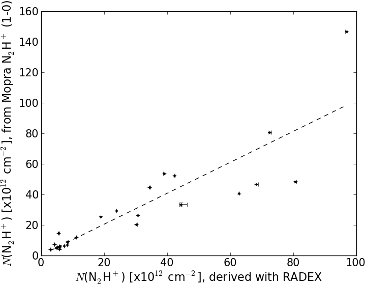
Figure 5: radex derived N₂H⁺ column density versus N₂H⁺ column density derived from the MOPRA N₂H⁺ (1–0) observations, using a 0.4 filling factor for both values. The dashed line represent the linear regression of the values. The slope of the linear regression is 1.01 meaning that the derived models on average represent a good approximation of the observed values.

4.2 Multiple Components

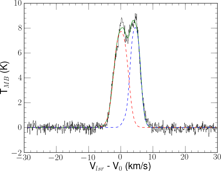
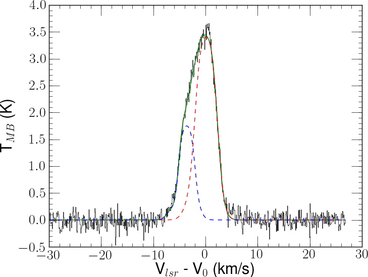
Figure 6: Two examples of N₂H⁺ (3–2) spectra, showing evidence of two velocity components. Both images show the N₂H⁺ (3–2) spectra overplotted with the two hyperfine component model fits (red and blue dashed lines) and the total model fit (green line). Top: SDC351.438, the two components seen clearly as a two-peaked feature. Bottom: L332-8, the two components are necessary to explain the broad feature of the N₂H⁺ (3–2) line.

Fig. 6 shows spectra of N₂H⁺ (3–2) towards two sources, which exhibit two velocity components. These spectra exemplify the two types of two-component spectra in the sample: Fig. 6 top (SDC351.438) shows a two-peaked feature, and Fig. 6 bottom (L332-8) shows a very broad feature which is likely due to two blended components. Two component features are seen in the N₂H⁺ (3–2) towards 13 of the 51 sources (25%).

There are several explanations for these two component lines. Optical depth effects could explain some of the sources. The more likely explanation however is the presence of multiple velocity components along the line of sight, as seen in high-mass star formation simulations (Smith et al. 2013) and in a number of observations (Csengeri et al. 2011; Beuther et al. 2013; Peretto et al. 2013).

There is no evidence to suggest that the presence of deuteration is correlated with the presence of multiple velocity components. Of the 28 objects with N₂H⁺ and N₂D⁺ (3–2) observations, eleven had two N₂H⁺ (3–2) components, ie (39%). Of the sources detected in N₂D⁺ (3–2) six of thirteen had two-velocity components, ie 46%. Chance of randomly selecting six or more two components out of 13 picks is 38%, consistent with a random selection.

In the remainder of the analysis, we associate the velocity component of N₂D⁺ with the NN₂H⁺ component closest in velocity.

4.3 Deuteration Ratio

The deuteration ratio, D${}_{\textrm{R}}$, is defined as the ratio of the column density of a deuterated species to its undeuterated counterpart. So for N₂H⁺,

$$\mathrm{D}_{R}=N\mathrm{(N_{2}D^{+})/}N\mathrm{(N_{2}H^{+})}.$$ (6)

Figure 7 shows the column density of N₂D⁺ versus the column density of N₂H⁺, overlaid with lines of constant D${}_{\textrm{R}}$ = 0.01, 0.04, and 0.25. Over the sample of objects with detected N₂D⁺, D${}_{\textrm{R}}$ has a mean of 0.024, a standard deviation of 0.037, and reaches a maximum value of 0.14. As we are using a filling factor of unity for N₂D⁺, the N₂D⁺ column density is a lower limit of the true value, thus the observed values of D${}_{\textrm{R}}$ is also a lower limit value. On the other hand the real average ratio may be lower because of the non-detections and upper limits in the sample.

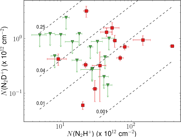
Figure 7: N₂H⁺ column density versus N₂D⁺ column density. Dashed lines are constant D${}_{\textrm{R}}$ ratio of 0.01, 0.04, and 0.25. Red squares represent detections, and green triangles represent upper limits of the N₂D⁺ column density.

4.3.1 Comparison with previous observations

Crapsi et al. (2005) did a survey of 31 low-mass starless cores in N₂H⁺ (1–0), N₂D⁺ (2–1), 13 of which had C¹⁸O, and 1.2mm continuum observations. Their main objective was to investigate the evolution of the cores. For this they used several methods, such as determining the abundance of N₂H⁺ and N₂D⁺, deuteration ratios, and CO depletion factors. For the mapped cores N₂H⁺ and N₂D⁺ peak close to the dust continuum maxima.

Emprechtinger et al. (2009) observed 20 class 0 protostars using the IRAM-30m telescope in various lines including N₂H⁺ (1–0) and N₂D⁺ (2–1). They determined the deuterium fractionation in order to analyse the chemical evolution of the objects. Compared with pre-stellar cores their class 0 objects had wider linewidths, higher excitation temperature and lower optical depth, consistent with the presence of a protostar. They found that D${}_{\textrm{R}}$ correlates with dust temperature, CO depletion factor, bolometric luminosity. This result is consistent with models where the maximum D${}_{\textrm{R}}$ is at the moment of collapse, and decreases as the heating of the protostar unfreezes the CO of the inner parts.

Fontani et al. (2011) took observations of 27 objects at different evolutionary stages of high-mass star formation process in N₂H⁺(3–2) and N₂D⁺(2–1). They studied high-mass starless cores candidates (HMSCs, 10 sources), high-mass protostellar objects (HMPOs, 10 objects), and ultra compact Hii regions (UCHiis, 7 objects). Their objective was to determine if the deuteration ratio is an evolutionary tracer in high mass regions as in low-mass regions. They found that the abundance of N₂D⁺ is higher in HMSCs than in HMPOs and UCHii regions, and that objects with highest deuteration ratio are starless cores. Their results indicate that D_R can be used as an evolutionary tracer in massive star forming regions, and that the physical conditions acting on the abundance of deuterated species likely evolve similarly in the low and high mass star formation processes.

Observations of the Spokes Cluster or NGC2264-D show supersonic turbulence in N₂H⁺ (1–0) (Peretto et al. 2006), however the fragmentation of most massive cores suggests that turbulence was not dominant. Pineda & Teixeira (2013) set out to determine if high density gas in NGC2264-D is subsonic or less turbulent, which would reconcile previous observations. They observed 14 cores in N₂H⁺ (3–2) and eight of them in N₂D⁺ (3–2) using APEX, in order to study the line widths and deuteration ratios. The N₂H⁺ and N₂D⁺ (3–2) show narrower line widths than N₂H⁺ (1–0). Three cores with no protostar show the highest level of deuteration, and are likely the youngest. They conclude that N₂H⁺ and N₂D⁺ (3–2) probe more quiescent gas and therefore is a better tracer of this gas in high-mass regions.

In Fig. 8 we compare our results and the results from Crapsi et al. (2005), Emprechtinger et al. (2009), Fontani et al. (2011), and Pineda & Teixeira (2013). The values of the column densities of Fontani et al. (2011) were recalculated using our procedure assuming equal filling factors, and we did not show objects that have only upper limits in N₂D⁺.

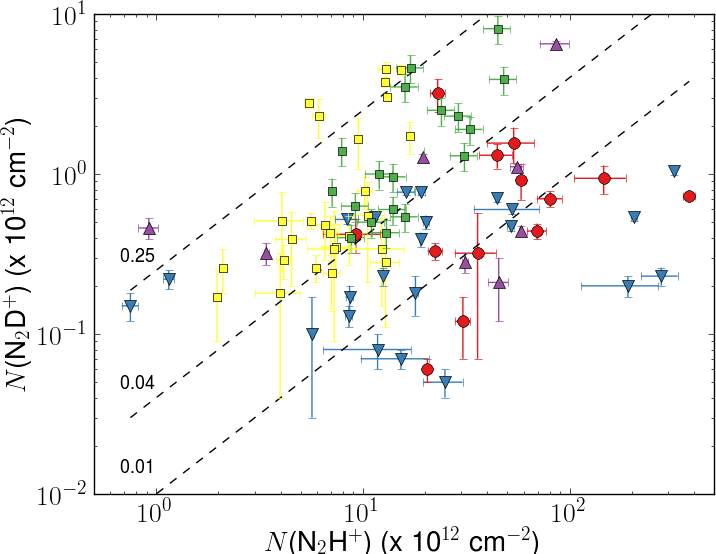
Figure 8: N₂H⁺ column density versus N₂D⁺ column density. Dashed lines are constant D${}_{\textrm{R}}$ ratio of 0.01, 0.04, and 0.25. Red circles = this paper. Purple upward triangles = Pineda & Teixeira (2013). Blue downward triangles = Fontani et al. (2011) (Recalculated values, upper limits not included). Yellow squares = Crapsi et al. (2005). Green squares = Emprechtinger et al. (2009).

As in Section 4 we use KS-tests and Student’s t-tests to investigate whether these samples have statistically different distributions. As expected, all except one of our regions have N₂H⁺ column density greater than all the low-mass sources of Crapsi et al. (2005), confirmed with the tests (p-values $<$ 0.01). In contrast the N₂D⁺ column densities are similar in both samples (p-values $>$ 0.1, we can not reject the null hypothesis of identical samples), which leads to the conclusion that our regions tend to have smaller deuteration ratios. On the other hand we are observing about the same range of N₂H⁺ and N₂D⁺ column densities as Fontani et al. (2011). Similarly we have about the same values for D${}_{\textrm{R}}$ as Fontani (p-values $>$ 0.5). A major factor in the differences in the samples is the distance at which they are observed, which influences the filling factor. Thus higher resolution observations are needed to provide more accurate values specially in the high-mass cases which are more distant.

We tested if D_R correlates with several parameters: the N₂H⁺ (1–0) integrated intensity, excitation temperature, optical depth, linewidth, N₂D⁺ (3–2) linewidth and N₂H⁺ column density. There is no clear correlation between D${}_{\textrm{R}}$ and any of these parameters. To quantify the linear correlation we calculated the Pearson-r parameter. The highest absolute value was 0.28 (for N₂H⁺ column density), a value low enough that is not statistically significantly different from zero.

4.4 Turbulence on smaller scales

Within low-mass star forming regions the turbulence decreases at smaller size scales and higher density (Fuller & Myers 1993; Pineda & Teixeira 2013). A smaller beam and the higher critical density of the 3–2 transition versus the 1–0 transition makes it interesting to investigate if high-mass star-forming regions show a similar trend.

Fig. 9 compares the velocity dispersions of N₂H⁺ (1–0) and N₂H⁺ (3–2). It shows that 16 of the 27 pointings have a smaller 3–2 linewidth. In fact, the N₂H⁺ (3–2) velocity dispersion is on average $\approx 78\%$ of the N₂H⁺ (1–0) dispersion. These results are consistent with Pineda & Teixeira (2013) who show that on average the N₂H⁺ (3–2) velocity dispersion is $\approx 70\%$ of the N₂H⁺ (1–0) dispersion. Further analysis of Fig. 9 could point out three possible sub-groups: the ones that follow the 0.78 relation, the ones above the identity line (i.e. velocity dispersion is higher in the 3–2 transition), and finally a group with very narrow lines (eight objects have $<40$%) in the 3–2 transition.

Fig. 10 compares the linewidth of N₂H⁺ (3–2) and N₂D⁺ (3–2), and it shows than N₂D⁺ (3–2) exhibits an even smaller linewidth for 11 of 13 pointings. On average the N₂D⁺ (3–2) velocity dispersion is $\approx 74\%$ of the N₂H⁺ (3–2) dispersion, with a typical N₂H⁺ (3–2) velocity dispersion of 0.63 km s^-1. This suggests that the N₂D⁺ (3–2) traces an even smaller and more quiescent region within the beam than the N₂H⁺ (3–2). In contrast, Pineda & Teixeira (2013) found almost no difference in linewidths between N₂H⁺ (3–2) and N₂D⁺ (3–2), the latter only 95% smaller.

However a more detailed analysis could suggest a different interpretation. In Fig. 10 there are three objects that are clearly separated, showing very narrow lines: SDC332.26A, SDC332.26B and SDC335.283. The spectra of these objects are well fitted, but for SDC335.283 the detection is just above 3$\sigma$. The lines are so narrow that they fall below the sound speed of an average molecule ($\approx$ 0.2 km s^-1 at 10 K and a mean molecular weight of 2.33). If we consider these three points as outliers, the mean ratio of linewidth between N₂H⁺ (3–2) and N₂D⁺ (3–2) is 96% which is concordance with the values seen by Pineda & Teixeira (2013). In addition it is interesting to note in Fig. 10 the clear dichotomy between objects with one or two velocity components in N₂H⁺ (3–2). The two velocity component objects have much higher linewidths while following the same trend.

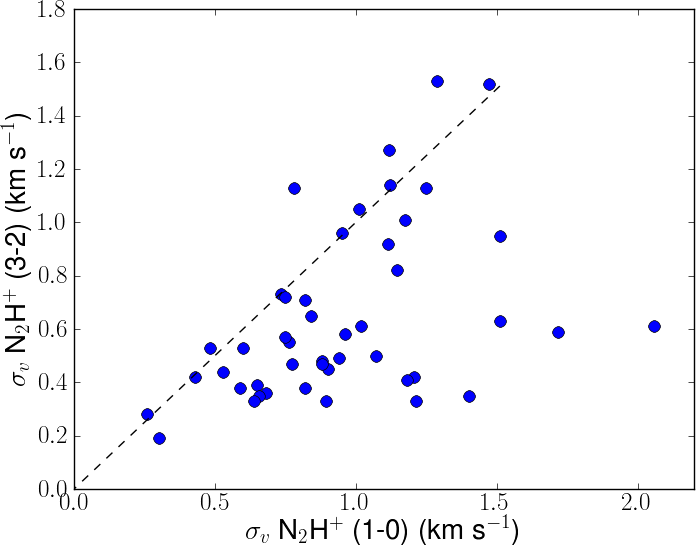
Figure 9: Comparison of the N₂H⁺ (1–0) linewidth (MOPRA) with the N₂H⁺ (3–2) linewidth (APEX). The dashed line represents the identity line.

Figure 10: Comparison of the N₂H⁺ (3–2) linewidth with the N₂D⁺ (3–2) linewidth. The blue dots and red squares indicate objects that exhibit one and two velocity components in the N₂H⁺ (3–2) spectra, respectively. The dashed line represents the identity line.

5 Discussion

5.1 Filling factor

The size of emission the regions of the N₂H⁺ and N₂D⁺ (3–2) transitions are likely to be different. The N₂D⁺ region is likely to be smaller because this species should be present only in the coldest and densest parts of the N₂H⁺ (3–2) region. This is consistent with high angular resolution observations.

Tan et al. (2013) observed six sources in N₂D⁺ (3–2) using ALMA and obtained a mean value for the size (diameter) of these cores of 0.11 pc with a maximum value of 0.175 pc. These sizes may be a lower limits as there may be flux loss in the interferometry data leading to a bias towards small structures. For the N₂D⁺ (3–2) APEX beam, and using 0.09 pc as the upper limit of the size for all the detected N₂D⁺ (3–2) sources, the calculated filling factors are 0.07 to 0.35 with a mean of 0.2. We have a filling factor corrected N₂H⁺ column density, applying this filling factors to the N₂D⁺ column densities, the deuteration ratio D${}_{\textrm{R}}$ increases by a factor of $\sim$ 5.0, highlighting the need of higher angular resolution to accurately constrain the deuteration in these regions.

Interferometer observations of N₂H⁺ 3–2 can also be used to estimate the filling factor. Chen et al. (2010) observed N₂H⁺ (3–2) in three regions using Submillimeter Array (SMA), and determined that the N₂H⁺ (3–2) was primarily in structures with size $\ga$ 0.2 pc. At the distance of our sources the APEX beam for N₂H⁺ (3–2) corresponds to linear sizes of 0.24–0.55 pc. Adopting a diameter for the N₂H⁺ (3–2) region of 0.2 pc we estimate beam filling factors for the detected N₂H⁺ (3–2) of between 0.13 and 0.67 with a mean of 0.38. Compared with the filling factor of unity adopted above this lower filling factor would increase the deuteration ratio by a factor $\sim$ 2, highlighting again the need of high angular resolution.

5.2 70 $\upmu$m content

We have used the HiGal 70 $\upmu$m observations to investigate the presence of young stellar objects (YSOs) in our sample (Peretto et al., in preparation). We determine the number of compact 70 $\upmu$m sources within the APEX beam by visual inspection. In the appendix (available online) we show the 70 $\upmu$m emission for the targets with N₂D⁺ (3–2) observations. 16 out of the 51 pointings have a 70 $\upmu$m source within the APEX beam. If we reduce the sample to those with N₂D⁺ (3–2) detections, six pointings have a 70 $\upmu$m source within the APEX beam.

The heating of material by a protostar should rapidly reduce any enhancement in the deuterium species as the CO unfreezes in the inner parts (Emprechtinger et al. 2009). Friesen et al. (2010) sees an anti-correlation between D${}_{\textrm{R}}$ and the distance to heating sources such as embedded protostars. So the presence of a 70 $\upmu$m source should inhibit the presence of N₂D⁺. But in our sample almost half (6 out of 13) of the objects with N₂D⁺ (3–2) detections have a 70 $\upmu$m source within the beam. There are two plausible scenarios for this incongruence. First there may be two distinct, different cores within beam; one with a heating source and little N₂D⁺, and one without a heating source but with N₂D⁺ emission. This scenario is consistent with the observations of two distinct components in the N₂H⁺ (3–2) emission, and the simulations showing that substructure (Smith et al. 2012). The other possibility is that we are seeing the phase after the start of the central heating but before the heating fully suppresses the N₂D⁺. So there may be a central region with no N₂D⁺, and an outer zone with pockets of N₂D⁺ being shielded by the central material and so still cold enough to maintain the deuterium enhancement. Distinguishing between these two possibilities require higher angular resolution observations.

The presence of a 70$\upmu$m source may affect the properties of the cloud, thus the properties observed in N₂H⁺ (1–0). To evaluate this possibility we separated into two samples; detections and non-detections of a 70$\upmu$m source within the beam, and performed statistical tests on the obtained line properties. Kolmogorov–Smirnov tests were evaluated for N₂H⁺ (1–0) velocity dispersion ($\sigma$), integrated intensity, column density, optical depth and excitation temperature ($T_{\text{ex}}$). For $\sigma$ and $T_{\text{ex}}$ we cannot reject the null hypothesis at a 0.05 level. This means that the presence of a 70$\upmu$m source is not affecting the linewidth or excitation temperature. The most significant difference is in the N₂H⁺ column density (Fig. 11). There are few sources with column densities less than 1.0 x 10¹² cm^-2 which contain 70 $\upmu$m sources. There are however regions without 70 $\upmu$m sources with high N₂H⁺ column densities similar to regions containing 70 $\upmu$m sources. These 13 sources with high column densities and no YSOs are regions of potentially high levels of deuteration, which should be investigated.

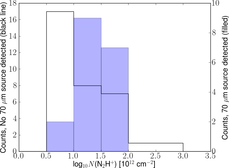
Figure 11: Histogram of N₂H⁺ column density for two subsamples: the filled histogram shows sources with a compact 70 $\upmu$m source within the APEX beam, and the black line is the histogram for sources without a 70 $\upmu$m source.

5.3 time-scales

Kong et al. (2015) used a gas-phase chemical model to investigate the evolution of the deuteration ratio with time, and the impact of various parameters on the time-scale. Their results can be compared with observations to provide information about the age of the cold dense gas. Their main fiducial model used typical values of low- and high-mass pre-stellar cores. They found that D_R increased with density and CO depletion factor, and decreased with temperature. In general, the model suggests that in order to reproduce the observed D${}_{\textrm{R}}$ values time-scales of several times the free-fall time-scale are required, meaning that the observed cores are dynamically old.

We compared the Kong et al. (2015) main fiducial model with our observations, in order to evaluate the degree of evolution of our sample. We had to convert the model’s N₂H⁺ and N₂D⁺ densities to column densities. For this we assumed a simple Gaussian density distribution with a peak value equal to the model density, and a width of 0.5 pc.

Fig. 12 shows a comparison of the Kong et al. (2015) models and our observations. The figure shows the column densities at different times, from 5 $\times$ 10⁴ yr to 3.2 $\times$ 10⁶ yr. The obtained values are only for one model, the fiducial model of their paper, with main parameter values: number density of H (n_H) = 10⁵ cm^-3, depletion factor (f${}_{\textrm{D}}$) = 10, cosmic ray ionization rate ($\zeta$) = 2.5 $\times$ 10^-17s^-1, temperature = 15 K and dust-to-gas ratio of 0.01. The values of the main model should provide a good first approximation to the objects. For example, Peretto et al. (2010) shows that the temperature of IRDCs is around 15 K. This model does a reasonable job in matching the observed values. A full exploration of the model parameters (plus size of core) should provide the whole range of observed values. The time corresponding to lowest observed D${}_{\textrm{R}}$ is $\sim$ 5.5 $\times$ 10⁵ years for the main model, which is about four times the free-fall time-scale for this model (1.39 $\times$ 10⁵ yr). So this approximation to the time-scales of our sample gives dynamically old cores for even the lowest observed D${}_{\textrm{R}}$. In addition to the main model, we consider three additional models: one with higher density, one with lower density, and one with increased depletion. As expected, given the models of Kong et al. (2015), varying the densities has a low impact on D${}_{\textrm{R}}$ mainly a small scaling effect. On the other hand the impact of a depletion factor 10 times higher is significant, D${}_{\textrm{R}}$ grows much quicker. For the lowest D${}_{\textrm{R}}$ it would only take 1.3 $\times$ 10⁵ yr to reach the observed value which is about the free-fall time-scale suggesting the cores have a short lifetime. On the other hand, the effect of the filling factor should increase the time-scales. More detailed or complex models are necessary to further understand the time evolution of the different cores.

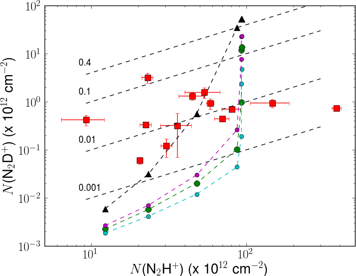
Figure 12: N₂H⁺ column density versus N₂D⁺ column density. Dashed lines are constant D${}_{\textrm{R}}$ ratio of 0.01, 0.04, and 0.25. Red squares represent our observed values. Green dots represent Kong et al. (2015) fiducial model (n = 10⁵ cm^-3, f${}_{\textrm{D}}$ = 10) converted values at different times, from 5 $\times$ 10⁴ yr to 3.2 $\times$ 10⁶ yr (each point is twice the age of the previous point). The lower and upper dot curves represent models with density of 10⁴ cm^-3 and 10⁶ cm^-3 respectively (f${}_{\textrm{D}}$ = 10). Black triangles are a model with a higher f_D = 100 (n = 10⁵ cm^-3).

6 Summary

In this paper we have presented the results of N₂H⁺ (1–0), N₂H⁺ (3–2) and N₂D⁺ (3–2) observations towards peaks in IRDCs. The main results of the paper are summarized as follows.

1. [i]

2. We have observed 54 cores towards IRDCs in N₂H⁺ (3–2) and 29 of them also in N₂D⁺ (3–2) with APEX, most of these are also observed in N₂H⁺ (1–0) with MOPRA. Our sample is the largest samples of N₂H⁺ and deuterium observations towards IRDCs to date.

3. The N₂H⁺ (3–2) spectra exhibit two velocity components in 25% of the sources. No source has two velocity components in N₂D⁺ (3–2).

4. N₂D⁺ (3–2) was detected towards 13 objects. Its detection does not correlate with the presence of two velocity components or any other N₂H⁺ (3–2) parameter except the excitation temperature. Sources detected in N₂D⁺ (3–2) show a higher $T_{\text{ex}}$ suggesting a higher density.

5. Modelling the N₂H⁺ lines we find a filling factor of 0.4 for the N₂H⁺ (1–0) transition, this implies a filling factor of unity for N₂H⁺ (3–2) and N₂D⁺ (3–2). We calculated the deuteration ratio, D${}_{\textrm{R}}$, and obtained values between 0.003 and 0.14. Using alternative estimates of the N₂D⁺ filling factor increases these values by a factor of at least $\sim$5.0. Compared with previous works, we observed in general higher N₂H⁺ column densities, especially compared with low-mass regions, however we find similar values of D${}_{\textrm{R}}$ compared with observations of high-mass regions by Fontani et al. (2011).

6. The measured velocity dispersions of N₂H⁺ (3–2) are in general narrower ($\approx$ 80%) than N₂H⁺ (1–0) with a typical N₂H⁺ (3–2) velocity dispersion 0.63 km s^-1. The situation comparing N₂D⁺ (3–2) and N₂H⁺ (3–2) is somewhat more complex as there are three outliers with very narrow N₂D⁺ (3–2) velocity dispersion. For the remainder of the sources the velocity dispersions are very similar in the two species and tend to be grouped around either 0.5 km s^-1 or 1.2 km s^-1.

7. The presence of a 70$\upmu$m source is not correlated with a detection of N₂D⁺ (3–2), which is surprising. In addition, the presence of a 70$\upmu$m source does not correlate with any change in linewidth and excitation temperature. However, sources with higher N₂H⁺ column density are more likely to be associated with the presence of a 70$\upmu$m source.

8. Comparison with the recent models of deuteration suggest evolutionary time-scales of these regions of several free-fall times or less. However the time-scales are highly dependant on the depletion factor of CO.

Our observations have shown that N₂H⁺ is widespread and a good tracer of the kinematics. N₂H⁺ and N₂D⁺ (3–2) motions are in general still supersonic even in the smallest regions traced in these observations. However, three intriguing regions appear to show subsonic turbulence in N₂D⁺ in marked contrast to the N₂H⁺. These regions deserve further investigation, as does the chemistry of the regions with a 70$\upmu$m source. In future more sophisticated models and higher resolution observations will help to better constrain the time-scales and evolution of these dense regions.

SUPPORTING INFORMATION

Additional Supporting Information may be found in the online version of this article:

Appendix_online.pdf (http://www.mnras.oxfordjournals.org/lookup/suppl/doi:10.1093/mnras/stv2354/-/DC1).

This paper has been typeset from a TEX/LATEX file prepared by the author.

Table 3: N₂H⁺ (1–0) parameters. The columns show in order: the source name, kinematic distance, N₂H⁺ (1–0) excitation temperature, local standard of rest velocity, linewidth, optical depth, integrated intensity, rms, and the derived column density (including the filling factor).

				N2H+ (1–0)
Source	Dist	$T_{\text{ex}}$	V${}_{\text{LSR}}$	$\sigma$	$\tau_{0}$	$\int Idv$	rms	$N$(N2H+)
	(kpc)	(K)	(km s-1)	(km s${}^{-1})$		(km s-1)	(mK)	(x1012cm-2)
SDC299.2	3.1	5.00$\pm$0.00	-38.96$\pm$0.12	0.68$\pm$0.13	0.36$\pm$0.06	1.11$\pm$0.12	91	4.02$\pm$1.02
SDC320.271	2.28	5.00$\pm$0.00	-32.23$\pm$0.06	0.88$\pm$0.07	0.63$\pm$0.05	2.40$\pm$0.12	90	9.10$\pm$1.02
SDC320.252	2.29	6.78$\pm$0.25	-32.50$\pm$0.01	0.78$\pm$0.02	3.03$\pm$0.40	14.81$\pm$1.65	92	80.61$\pm$11.21
SDC321.708	2.33	5.00$\pm$0.00	-32.57$\pm$0.06	1.07$\pm$0.06	1.31$\pm$0.08	5.57$\pm$0.22	151	23.01$\pm$1.91
SDC321.758	2.26	5.11$\pm$0.16	-31.78$\pm$0.02	0.60$\pm$0.03	4.29$\pm$0.74	8.53$\pm$1.07	83	44.71$\pm$8.15
SDC321.936	2.27	5.00$\pm$0.00	-31.94$\pm$0.02	0.84$\pm$0.03	4.33$\pm$0.21	10.97$\pm$0.20	119	59.70$\pm$3.60
SDC329.028	2.92	3.97$\pm$0.05	-44.39$\pm$0.05	1.51$\pm$0.04	4.98$\pm$0.52	10.59$\pm$0.81	88	69.66$\pm$7.55
SDC329.068	2.81	4.39$\pm$0.19	-43.26$\pm$0.07	1.72$\pm$0.06	2.35$\pm$0.46	9.96$\pm$1.89	104	48.22$\pm$9.94
SDC329.186	3.19	5.00$\pm$0.00	-50.80$\pm$0.05	1.29$\pm$0.04	1.32$\pm$0.05	6.69$\pm$0.29	87	27.88$\pm$1.36
SDC329.313	4.35	26.87$\pm$0.80	-73.59$\pm$0.03	0.90$\pm$0.04	0.10$\pm$0.00	4.87$\pm$0.12	85	58.28$\pm$3.32
SDC351.438	3.1	9.43$\pm$0.20	-5.15$\pm$0.02	1.47$\pm$0.02	3.53$\pm$0.22	49.88$\pm$2.63	221	379.47$\pm$25.31
SDC352.027	3.1	5.22$\pm$0.22	2.32$\pm$0.03	0.65$\pm$0.04	4.52$\pm$1.11	9.93$\pm$1.69	153	53.65$\pm$13.78
SDC351.8	3.1	5.00$\pm$0.00	-0.81$\pm$0.03	0.26$\pm$0.02	1.52$\pm$0.14	1.62$\pm$0.09	97	6.49$\pm$0.78
SDC351.562	3.1	5.00$\pm$0.00	-2.70$\pm$0.04	0.43$\pm$0.04	20.73$\pm$5.44	13.37$\pm$0.55	324	146.31$\pm$40.74
L332-10	3.2	5.00$\pm$0.00	-48.21$\pm$0.06	0.74$\pm$0.06	0.68$\pm$0.05	2.17$\pm$0.24	73	8.24$\pm$0.97
L332-11	3.32	5.00$\pm$0.00	-49.85$\pm$0.08	0.75$\pm$0.09	0.41$\pm$0.04	1.37$\pm$0.22	66	5.04$\pm$0.84
L332-12	3.16	5.00$\pm$0.00	-47.92$\pm$0.12	1.12$\pm$0.12	0.34$\pm$0.03	1.69$\pm$0.24	75	6.22$\pm$0.91
L332-13	3.18	5.00$\pm$0.00	-48.04$\pm$0.09	0.82$\pm$0.10	0.52$\pm$0.06	1.89$\pm$0.29	88	7.07$\pm$1.14
L332-14	3.26	5.00$\pm$0.00	-49.12$\pm$0.11	0.89$\pm$0.12	0.36$\pm$0.04	1.44$\pm$0.26	78	5.30$\pm$0.97
L332-15	3.23	15.30$\pm$0.74	-48.58$\pm$0.06	0.94$\pm$0.07	0.10$\pm$0.00	2.61$\pm$0.25	76	18.30$\pm$1.77
L332-1	3.13	5.00$\pm$0.00	-46.76$\pm$0.10	0.48$\pm$0.11	1.16$\pm$0.25	2.35$\pm$0.67	221	9.24$\pm$2.85
L332-3	3.29	16.02$\pm$1.70	-50.00$\pm$0.09	-0.68$\pm$0.11	0.10$\pm$0.00	1.99$\pm$0.41	125	14.59$\pm$3.05
L332-4	3.33	5.00$\pm$0.00	-50.43$\pm$0.25	1.21$\pm$0.25	0.21$\pm$0.04	1.14$\pm$0.31	96	4.11$\pm$1.12
L332-5	3.19	5.00$\pm$0.00	-48.93$\pm$0.15	0.96$\pm$0.16	0.39$\pm$0.06	1.67$\pm$0.36	109	6.19$\pm$1.36
L332-6	3.29	5.00$\pm$0.00	-49.89$\pm$0.10	0.66$\pm$0.12	0.47$\pm$0.07	1.36$\pm$0.31	94	5.05$\pm$1.19
L332-7	3.19	4.41$\pm$0.30	-48.75$\pm$0.05	1.01$\pm$0.06	2.28$\pm$0.68	6.02$\pm$1.81	111	27.83$\pm$8.66
L332-8	3.16	5.07$\pm$0.32	-47.68$\pm$0.03	1.12$\pm$0.04	1.89$\pm$0.40	8.11$\pm$1.83	91	35.90$\pm$8.09
L332-9	3.16	5.00$\pm$0.00	-47.62$\pm$0.04	1.12$\pm$0.03	1.11$\pm$0.04	5.07$\pm$0.21	62	20.53$\pm$0.91
SDC335.283A	3.13	17.47$\pm$0.75	-44.87$\pm$0.07	1.18$\pm$0.07	0.10$\pm$0.00	3.84$\pm$0.31	95	30.48$\pm$2.49
SDC335.283B	3.09	11.13$\pm$1.12	-44.75$\pm$0.14	0.95$\pm$0.16	0.10$\pm$0.00	1.73$\pm$0.38	114	9.18$\pm$2.02
SDC335.077A	2.87	14.75$\pm$0.62	-39.52$\pm$0.08	1.25$\pm$0.08	0.10$\pm$0.00	3.30$\pm$0.27	83	22.43$\pm$1.85
SDC335.077B	3.1	9.14$\pm$0.65	-38.55$\pm$0.15	1.19$\pm$0.14	0.10$\pm$0.00	1.64$\pm$0.26	82	7.41$\pm$1.20
SDC335.579A	3.19	4.32$\pm$0.16	-46.38$\pm$0.04	1.15$\pm$0.04	2.52$\pm$0.44	6.88$\pm$1.19	78	33.06$\pm$6.09
SDC335.579B	3.28	5.00$\pm$0.00	-47.10$\pm$0.10	0.88$\pm$0.11	0.39$\pm$0.04	1.52$\pm$0.24	73	5.61$\pm$0.91
SDC335.579Y1	3.26	5.02$\pm$0.19	-46.44$\pm$0.03	1.21$\pm$0.03	2.32$\pm$0.32	10.00$\pm$1.39	84	46.54$\pm$6.84
SDC335.579Y2	3.21	4.80$\pm$0.19	-46.44$\pm$0.03	1.18$\pm$0.03	2.32$\pm$0.35	8.83$\pm$1.34	81	40.95$\pm$6.51
SDC335.44	3.11	8.23$\pm$0.62	-45.18$\pm$0.32	2.06$\pm$0.25	0.10$\pm$0.00	2.41$\pm$0.40	102	10.04$\pm$1.70
SDC335.253	3.1	5.01$\pm$0.00	-45.22$\pm$0.17	0.78$\pm$0.19	0.40$\pm$0.08	1.40$\pm$0.44	130	5.17$\pm$1.66
SDC335.229A	3.11	12.33$\pm$0.94	-40.12$\pm$0.17	1.40$\pm$0.16	0.10$\pm$0.00	2.94$\pm$0.44	137	17.01$\pm$2.60
SDC335.229B	2.88	-	-	-	-	-	-	-
SDC335.059	2.84	15.28$\pm$1.85	-39.30$\pm$0.10	-0.61$\pm$0.11	0.10$\pm$0.00	1.68$\pm$0.39	122	11.78$\pm$2.82
SDC356.84	3.44	5.00$\pm$0.00	-7.94$\pm$0.05	0.82$\pm$0.06	1.10$\pm$0.08	3.71$\pm$0.15	110	14.81$\pm$1.53
SDC13.174A	3.6	5.00$\pm$0.00	37.12$\pm$0.06	0.77$\pm$0.06	0.94$\pm$0.07	3.04$\pm$0.31	93	11.93$\pm$1.30
SDC13.174B	3.1	5.00$\pm$0.00	37.36$\pm$0.11	0.54$\pm$0.12	0.38$\pm$0.08	0.92$\pm$0.28	90	3.38$\pm$1.05
SDC13.194	3.57	5.00$\pm$0.00	36.41$\pm$0.11	0.76$\pm$0.12	0.43$\pm$0.06	1.47$\pm$0.31	92	5.45$\pm$1.17
SDC16.915	3.41	5.00$\pm$0.00	41.30$\pm$0.04	0.64$\pm$0.04	2.42$\pm$0.18	5.69$\pm$0.19	140	25.42$\pm$2.47
SDC2.141	2.68	3.96$\pm$0.06	4.66$\pm$0.04	0.53$\pm$0.04	10.68$\pm$2.55	6.34$\pm$0.60	121	52.34$\pm$13.13
SDC2.116	2.36	5.00$\pm$0.00	3.88$\pm$0.05	0.75$\pm$0.06	1.45$\pm$0.11	4.29$\pm$0.18	134	17.85$\pm$1.97
SDC301.876	3.1	3.43$\pm$0.05	-43.15$\pm$0.03	0.30$\pm$0.03	17.17$\pm$5.18	2.81$\pm$0.32	92	33.03$\pm$10.51
SDC327.894	2.93	3.72$\pm$0.08	-44.48$\pm$0.04	0.59$\pm$0.05	6.33$\pm$1.76	4.20$\pm$0.67	93	29.36$\pm$8.56
SDC327.964	2.97	5.00$\pm$0.00	-44.85$\pm$0.03	0.42$\pm$0.04	1.05$\pm$0.09	1.89$\pm$0.08	73	7.24$\pm$0.93
SDC34.558	3.33	18.15$\pm$1.37	53.19$\pm$0.17	1.51$\pm$0.14	0.10$\pm$0.00	5.17$\pm$0.38	267	42.49$\pm$5.64
SDC37.08	5.13	5.00$\pm$0.00	81.70$\pm$0.06	1.02$\pm$0.06	1.57$\pm$0.10	6.19$\pm$0.24	168	26.29$\pm$2.28

Table 4: N₂H⁺ (3–2) parameters. The columns show in order: the source name, the N₂H⁺ (3–2) excitation temperature, local standard of rest velocity, linewidth, optical depth, integrated intensity, rms, and the derived column density.

				N2H+ (3–2)
Source	$T_{\text{ex}}$	V${}_{\text{LSR}}$	$\sigma$	$\tau_{0}$	$\int Idv$	rms	$N$(N2H+)
	(K)	(km s-1)	(km s${}^{-1})$		(km s-1)	(mK)	(x1012cm-2)
SDC299.2	6.50$\pm$0.00	-39.69$\pm$0.03	0.36$\pm$0.03	0.24$\pm$0.02	0.39$\pm$0.03	68	1.48$\pm$0.17
SDC320.271	3.66$\pm$0.04	-32.44$\pm$0.05	0.48$\pm$0.04	9.75$\pm$2.30	0.77$\pm$0.06	52	219.32$\pm$74.64
SDC320.252-a	9.22$\pm$0.00	-32.36$\pm$0.01	1.13$\pm$0.01	1.83$\pm$0.03	12.55$\pm$0.28	203	29.97$\pm$0.56
SDC320.252-b	9.22$\pm$0.00	-35.72$\pm$0.02	0.52$\pm$0.02	0.42$\pm$0.01	1.94$\pm$0.28	203	3.17$\pm$0.14
SDC321.708	4.47$\pm$0.03	-33.50$\pm$0.02	0.50$\pm$0.02	6.27$\pm$0.95	1.61$\pm$0.08	76	91.11$\pm$17.67
SDC321.758	5.57$\pm$0.04	-32.29$\pm$0.02	0.53$\pm$0.02	6.93$\pm$0.78	3.60$\pm$0.12	117	74.20$\pm$11.32
SDC321.936	8.48$\pm$0.02	-32.52$\pm$0.01	0.65$\pm$0.01	14.20$\pm$0.38	14.91$\pm$0.10	325	135.77$\pm$4.94
SDC329.028-a	11.12$\pm$0.00	-42.00$\pm$0.01	0.95$\pm$0.01	2.61$\pm$0.05	18.39$\pm$1.33	155	36.46$\pm$0.80
SDC329.028-b	9.37$\pm$0.22	-46.41$\pm$0.02	1.44$\pm$0.04	1.92$\pm$0.23	16.81$\pm$1.33	155	40.02$\pm$8.38
SDC329.068-a	4.61$\pm$0.06	-40.59$\pm$0.05	0.59$\pm$0.03	17.48$\pm$2.73	2.94$\pm$0.53	95	282.10$\pm$76.15
SDC329.068-b	4.35$\pm$0.06	-43.66$\pm$0.09	0.95$\pm$0.12	7.33$\pm$3.01	2.64$\pm$0.53	95	59.44$\pm$21.22
SDC329.186-a	6.46$\pm$0.20	-50.73$\pm$0.08	1.53$\pm$0.10	4.72$\pm$1.19	11.62$\pm$2.31	144	123.97$\pm$54.01
SDC329.186-b	7.51$\pm$0.14	-48.68$\pm$0.04	1.21$\pm$0.04	6.23$\pm$0.69	14.65$\pm$2.31	144	116.30$\pm$24.52
SDC329.313	5.38$\pm$0.03	-73.87$\pm$0.02	0.45$\pm$0.01	17.53$\pm$1.24	3.96$\pm$0.10	133	167.08$\pm$17.91
SDC351.438-a	14.99$\pm$0.00	-6.07$\pm$0.04	1.52$\pm$0.03	1.95$\pm$0.03	39.77$\pm$1.56	387	50.10$\pm$1.25
SDC351.438-b	14.99$\pm$0.00	-1.64$\pm$0.03	1.08$\pm$0.01	2.26$\pm$0.07	31.13$\pm$1.56	387	41.26$\pm$1.33
SDC352.027	4.96$\pm$0.04	1.97$\pm$0.02	0.39$\pm$0.01	10.65$\pm$1.21	2.29$\pm$0.09	96	99.68$\pm$16.85
SDC351.8	6.50$\pm$0.00	-1.18$\pm$0.03	0.28$\pm$0.03	0.25$\pm$0.02	0.31$\pm$0.02	51	1.20$\pm$0.16
SDC351.562	5.56$\pm$0.03	-3.13$\pm$0.01	0.42$\pm$0.01	13.53$\pm$0.92	3.74$\pm$0.09	122	115.08$\pm$11.74
L332-10	7.72$\pm$0.33	-48.32$\pm$0.08	0.73$\pm$0.08	0.10$\pm$0.00	0.49$\pm$0.04	71	1.08$\pm$0.53
L332-11	6.50$\pm$0.00	-50.94$\pm$0.05	0.72$\pm$0.05	0.25$\pm$0.02	0.76$\pm$0.04	70	3.07$\pm$0.33
L332-12	9.38$\pm$0.26	-47.57$\pm$0.06	0.92$\pm$0.06	0.10$\pm$0.00	0.92$\pm$0.04	71	1.29$\pm$0.33
L332-13	4.76$\pm$0.07	-48.06$\pm$0.03	0.38$\pm$0.03	5.30$\pm$1.41	1.47$\pm$0.14	122	51.91$\pm$18.83
L332-14	4.12$\pm$0.05	-49.55$\pm$0.03	0.33$\pm$0.03	7.66$\pm$2.02	0.88$\pm$0.08	71	87.64$\pm$31.44
L332-15	5.19$\pm$0.04	-48.86$\pm$0.02	0.49$\pm$0.02	11.29$\pm$1.15	3.24$\pm$0.10	113	123.51$\pm$19.31
L332-1	6.32$\pm$0.03	-46.81$\pm$0.02	0.53$\pm$0.01	17.31$\pm$0.88	6.99$\pm$0.12	167	160.72$\pm$12.40
L332-3	5.84$\pm$0.04	-50.19$\pm$0.01	0.38$\pm$0.01	14.48$\pm$1.04	4.05$\pm$0.10	149	104.83$\pm$12.12
L332-4	6.50$\pm$0.00	-50.93$\pm$0.03	0.33$\pm$0.03	0.58$\pm$0.05	0.77$\pm$0.05	121	3.27$\pm$0.41
L332-5	6.50$\pm$0.00	-47.98$\pm$0.05	0.58$\pm$0.05	0.24$\pm$0.02	0.60$\pm$0.04	68	2.38$\pm$0.28
L332-6	4.88$\pm$0.05	-50.08$\pm$0.02	0.35$\pm$0.02	9.13$\pm$1.50	1.88$\pm$0.10	122	78.83$\pm$18.55
L332-7-a	10.89$\pm$0.00	-48.03$\pm$0.01	1.05$\pm$0.01	2.35$\pm$0.03	18.49$\pm$5.61	236	36.12$\pm$0.58
L332-7-b	6.21$\pm$1.22	-51.42$\pm$0.05	0.75$\pm$0.09	0.96$\pm$0.96	2.26$\pm$5.61	236	9.74$\pm$36.64
L332-8-a	8.83$\pm$0.00	-46.83$\pm$0.09	1.27$\pm$0.04	2.84$\pm$0.12	16.16$\pm$2.34	111	52.58$\pm$2.77
L332-8-b	6.52$\pm$0.15	-50.54$\pm$0.13	0.92$\pm$0.06	3.02$\pm$0.67	6.37$\pm$2.34	111	47.31$\pm$16.35
L332-9	22.91$\pm$0.32	-47.58$\pm$0.02	1.14$\pm$0.02	0.10$\pm$0.00	4.64$\pm$0.08	101	2.75$\pm$0.13
SDC335.283A-a	8.21$\pm$0.00	-44.30$\pm$0.06	1.01$\pm$0.02	2.37$\pm$0.12	10.34$\pm$2.89	130	35.55$\pm$1.93
SDC335.283A-b	5.07$\pm$0.07	-47.39$\pm$0.16	0.82$\pm$0.07	4.43$\pm$1.24	3.36$\pm$2.89	130	84.12$\pm$30.04
SDC335.283B	6.50$\pm$0.00	-43.97$\pm$0.05	0.96$\pm$0.05	0.44$\pm$0.02	1.71$\pm$0.07	101	7.21$\pm$0.50
SDC335.077A-a	10.40$\pm$0.00	-39.40$\pm$0.03	1.13$\pm$0.02	1.33$\pm$0.04	12.92$\pm$9.15	352	21.83$\pm$0.76
SDC335.077A-b	5.59$\pm$0.08	-41.34$\pm$0.06	0.92$\pm$0.05	7.33$\pm$1.45	5.81$\pm$9.15	352	135.61$\pm$37.94
SDC335.077B	-	-	-	-	-	40	0.7a
SDC335.579A-a	5.94$\pm$0.00	-44.80$\pm$0.05	0.82$\pm$0.04	1.68$\pm$0.10	3.25$\pm$1.31	140	25.74$\pm$1.98
SDC335.579A-b	5.23$\pm$0.16	-47.11$\pm$0.04	0.45$\pm$0.04	3.03$\pm$1.04	1.79$\pm$1.31	140	15.46$\pm$13.96
SDC335.579B	4.29$\pm$0.03	-47.71$\pm$0.03	0.47$\pm$0.02	16.19$\pm$1.79	1.83$\pm$0.07	77	240.98$\pm$41.41
SDC335.579Y1-a	6.86$\pm$0.04	-44.19$\pm$0.01	0.42$\pm$0.01	17.09$\pm$0.87	7.10$\pm$0.24	375	117.29$\pm$9.76
SDC335.579Y1-b	12.31$\pm$0.03	-47.58$\pm$0.01	0.79$\pm$0.01	9.36$\pm$0.22	30.27$\pm$0.24	375	112.36$\pm$3.30
SDC335.579Y2-a	8.10$\pm$0.05	-44.19$\pm$0.01	0.41$\pm$0.01	10.58$\pm$0.46	8.34$\pm$0.41	257	64.72$\pm$4.72
SDC335.579Y2-b	10.73$\pm$0.00	-47.44$\pm$0.01	1.43$\pm$0.01	1.49$\pm$0.02	18.44$\pm$0.41	257	31.10$\pm$0.47
SDC335.44	4.90$\pm$0.04	-44.35$\pm$0.04	0.61$\pm$0.02	16.60$\pm$1.76	3.65$\pm$0.11	121	248.06$\pm$41.59
SDC335.253	-	-	-	-	-	41	0.71a
SDC335.229A-a	3.39$\pm$0.06	-40.07$\pm$0.08	0.35$\pm$0.06	13.09$\pm$6.11	0.43$\pm$0.13	68	62.08$\pm$37.36
SDC335.229A-b	3.85$\pm$0.00	-44.46$\pm$0.06	0.39$\pm$0.06	1.54$\pm$0.34	0.34$\pm$0.13	68	24.58$\pm$6.61
SDC335.229B	6.50$\pm$0.00	-39.92$\pm$0.07	0.63$\pm$0.06	0.27$\pm$0.03	0.72$\pm$0.06	102	2.90$\pm$0.42

Table 5: N₂H⁺ (3–2) parameters continued.

				N2H+ (3–2)	(continuation)
Source	$T_{\text{ex}}$	V${}_{\text{LSR}}$	$\sigma$	$\tau_{0}$	$\int Idv$	rms	$N$(N2H+)
	(K)	(km s-1)	(km s${}^{-1})$		(km s-1)	(mK)	(x1012cm-2)
SDC335.059	6.50$\pm$0.00	-39.19$\pm$0.20	0.66$\pm$0.20	0.05$\pm$0.01	0.16$\pm$0.04	38	0.58$\pm$0.14
SDC356.84	6.50$\pm$0.00	-8.48$\pm$0.06	0.71$\pm$0.06	0.22$\pm$0.02	0.67$\pm$0.04	57	2.67$\pm$0.33
SDC13.174A	4.47$\pm$0.05	36.90$\pm$0.03	0.47$\pm$0.03	6.24$\pm$1.39	1.53$\pm$0.11	80	85.23$\pm$25.56
SDC13.174B	-	-	-	-	-	99	1.72a
SDC13.194	6.50$\pm$0.00	36.42$\pm$0.04	0.55$\pm$0.04	0.31$\pm$0.02	0.73$\pm$0.04	63	2.91$\pm$0.28
SDC16.915	4.76$\pm$0.05	40.90$\pm$0.02	0.33$\pm$0.01	16.75$\pm$2.06	2.04$\pm$0.10	109	142.47$\pm$29.86
SDC2.141	6.50$\pm$0.00	4.27$\pm$0.02	0.44$\pm$0.02	0.55$\pm$0.03	0.96$\pm$0.04	155	4.13$\pm$0.29
SDC2.116	6.50$\pm$0.00	3.52$\pm$0.03	0.57$\pm$0.03	0.34$\pm$0.02	0.83$\pm$0.04	70	3.31$\pm$0.26
SDC301.876	4.27$\pm$0.06	-43.27$\pm$0.02	0.19$\pm$0.02	9.20$\pm$2.37	0.70$\pm$0.06	75	55.92$\pm$20.97
SDC327.894	3.95$\pm$0.04	-44.52$\pm$0.03	0.38$\pm$0.02	11.74$\pm$2.33	0.97$\pm$0.07	70	171.10$\pm$48.69
SDC327.964	6.50$\pm$0.00	-45.23$\pm$0.07	0.50$\pm$0.07	0.14$\pm$0.02	0.32$\pm$0.03	66	1.20$\pm$0.24
SDC34.558	6.50$\pm$0.00	52.73$\pm$0.03	0.63$\pm$0.03	0.36$\pm$0.02	0.95$\pm$0.04	73	3.87$\pm$0.28
SDC37.08	5.42$\pm$0.03	81.50$\pm$0.02	0.61$\pm$0.02	15.43$\pm$1.12	4.87$\pm$0.10	138	197.29$\pm$21.75

Note. ^adenotes upper limit.

Table 6: N₂D⁺ (3–2) parameters. The columns show in order: the source name, the N₂D⁺ (3–2) local standard of rest velocity, linewidth, optical depth, integrated intensity, rms, the derived column density, and the deuteration ratio

			N2D+ (3–2)
Source	V${}_{\text{LSR}}$	$\sigma$	$\tau_{0}$	$\int Idv$	$rms$	$N$(N2D+)	DR
	(K)	(km s${}^{-1})$		(km s${}^{-1})$	(mK)	(x1012cm-2)
SDC320.252-a	-32.60$\pm$0.17	1.28$\pm$0.17	0.03$\pm$0.00	0.42$\pm$0.04	34	0.70$\pm$0.08	0.009
SDC321.708	-32.75$\pm$0.07	0.40$\pm$0.07	0.41$\pm$0.07	0.31$\pm$0.04	39	3.19$\pm$0.74	0.139
SDC321.758	-31.22$\pm$0.06	0.47$\pm$0.06	0.18$\pm$0.02	0.31$\pm$0.03	33	1.31$\pm$0.23	0.029
SDC329.028-a	-43.66$\pm$0.17	1.12$\pm$0.17	0.02$\pm$0.00	0.35$\pm$0.04	32	0.44$\pm$0.05	0.006
SDC329.068-a	-	-	-	-	36	1.01a	0.021
SDC329.186-a	-	-	-	-	53	0.28a	0.010
SDC329.313	-73.42$\pm$0.12	0.48$\pm$0.13	0.11$\pm$0.03	0.19$\pm$0.04	41	0.92$\pm$0.23	0.016
SDC351.438-a	-3.88$\pm$0.11	1.50$\pm$0.12	0.02$\pm$0.00	0.88$\pm$0.05	35	0.73$\pm$0.04	0.002
SDC352.027	2.50$\pm$0.07	0.37$\pm$0.08	0.24$\pm$0.05	0.24$\pm$0.03	32	1.56$\pm$0.39	0.029
SDC351.562	-2.64$\pm$0.08	0.37$\pm$0.09	0.16$\pm$0.03	0.22$\pm$0.03	39	0.94$\pm$0.19	0.006
L332-10	-	-	-	-	67	0.48a	0.058
L332-13	-	-	-	-	39	1.23a	0.174
L332-15	-	-	-	-	55	1.22a	0.067
L332-1	-46.66$\pm$0.10	0.35$\pm$0.12	0.08$\pm$0.02	0.15$\pm$0.03	40	0.42$\pm$0.10	0.045
L332-3	-	-	-	-	59	0.87a	0.060
L332-6	-	-	-	-	41	1.16a	0.230
L332-7a	-	-	-	-	58	0.27a	0.010
L332-8a	-47.75$\pm$0.03	0.07$\pm$0.04	0.28$\pm$0.37	0.20$\pm$0.15	24	0.32$\pm$0.25	0.009
L332-9	-46.72$\pm$0.05	0.10$\pm$0.06	0.02$\pm$0.01	0.09$\pm$0.02	37	0.06$\pm$0.01	0.003
SDC335.283A-a	-44.36$\pm$0.08	0.11$\pm$0.04	0.06$\pm$0.02	0.07$\pm$0.02	37	0.12$\pm$0.05	0.004
SDC335.077A-a	-39.14$\pm$0.15	0.92$\pm$0.14	0.02$\pm$0.00	0.27$\pm$0.03	32	0.33$\pm$0.04	0.015
SDC335.579A-a	-	-	-	-	43	0.88a	0.027
SDC335.579Y1-a	-	-	-	-	39	0.14a	0.003
SDC335.579Y2-a	-	-	-	-	38	0.20a	0.005
SDC335.44	-	-	-	-	42	1.17a	0.117
SDC335.229A-a	-	-	-	-	37	0.40a	0.024
SDC13.174A	-	-	-	-	58	2.42a	0.203
SDC34.558	-	-	-	-	43	0.46a	0.011
SDC37.08	-	-	-	-	37	0.70a	0.027

Note. ^adenotes upper limit.

References

- Beuther et al. (2013) Beuther H., Linz H., Tackenberg J., Henning T., Krause O., Ragan S., Nielbock M., Launhardt R., Bihr S., Schmiedeke A., Smith R., Sakai T., 2013, A&A, 553, A115
- Carey et al. (1998) Carey S. J., Clark F. O., Egan M. P., Price S. D., Shipman R. F., Kuchar T. A., 1998, ApJ, 508, 721
- Carey et al. (2000) Carey S. J., Feldman P. A., Redman R. O., Egan M. P., MacLeod J. M., Price S. D., 2000, ApJ, 543, L157
- Caselli et al. (2002) Caselli P., Walmsley C. M., Zucconi A., Tafalla M., Dore L., Myers P. C., 2002, ApJ, 565, 344
- Chen et al. (2010) Chen H.-R., Liu S.-Y., Su Y.-N., Zhang Q., 2010, ApJ, 713, L50
- Crapsi et al. (2005) Crapsi A., Caselli P., Walmsley C. M., Myers P. C., Tafalla M., Lee C. W., Bourke T. L., 2005, ApJ, 619, 379
- Csengeri et al. (2011) Csengeri T., Bontemps S., Schneider N., Motte F., Dib S., 2011, A&A, 527, A135
- Egan et al. (1998) Egan M. P., Shipman R. F., Price S. D., Carey S. J., Clark F. O., Cohen M., 1998, ApJ, 494, L199