Asymptotic Distribution and Detection Thresholds for Two-Sample Tests Based on Geometric Graphs

Abstract.

In this paper, we consider the problem of testing the equality of two multivariate distributions based on geometric graphs constructed using the interpoint distances between the observations. These include the tests based on the minimum spanning tree and the $K$-nearest neighbor (NN) graphs, among others. These tests are asymptotically distribution-free, universally consistent and computationally efficient, making them particularly useful in modern applications. However, very little is known about the power properties of these tests. In this paper, using the theory of stabilizing geometric graphs, we derive the asymptotic distribution of these tests under general alternatives, in the Poissonized setting. Using this, the detection threshold and the limiting local power of the test based on the $K$-NN graph are obtained, where interesting exponents depending on dimension emerge. This provides a way to compare and justify the performance of these tests in different examples.

1. Introduction

Given independent and identically distributed samples

$$\mathscr{X}_{N_{1}}=\{X_{1},X_{2},\ldots,X_{N_{1}}\}\quad\text{and}\quad\mathscr{Y}_{N_{2}}=\{Y_{1},Y_{2},\ldots,Y_{N_{2}}\},$$ (1.1)

from two unknown densities $f$ and $g$ (with respect to the Lebesgue measure) in $\mathbb{R}^{d}$, respectively, the two-sample problem is to test the hypotheses

$$H_{0}:f=g\quad\text{versus}\quad H_{1}:f\neq g.$$ (1.2)

In this paper, we will derive asymptotic properties of two-sample tests based on geometric graphs in the usual limiting regime where the dimension $d$ is fixed and the sample size $N_{1}+N_{2}:=N\rightarrow\infty$, such that

$$\frac{N_{1}}{N_{1}+N_{2}}\rightarrow p\in(0,1),\qquad\frac{N_{2}}{N_{1}+N_{2}}\rightarrow q:=1-p.$$ (1.3)

For univariate data, there are several well-known nonparametric tests such as the two-sample Kolmogorov–Smirnoff maximum deviation test [30], the Wald–Wolfowitz runs test [32] and the Mann–Whitney rank test [22].

The nonparametric two-sample problem for multivariate data has been extensively studied, beginning with the work of Weiss [33] and Bickel [9]. Friedman and Rafsky [14] generalized the Wald–Wolfowitz runs test [32] to higher dimensions using the Euclidean minimal spanning tree (MST) of the pooled data. Thereafter, many other two-sample tests based on geometric graphs have been proposed. Schilling [29] and Henze [18] considered tests based on the $K$-nearest neighbor ($K$-NN) graph of the pooled sample. Later, Rosenbaum [26] developed a test based on matchings, and, more recently, Biswas et al. [10] proposed a test based on the Hamiltonian cycle, both of which are exactly distribution-free under the null. Recently, Chen and Friedman [11] proposed new modifications of these tests for high-dimensional and object data. Maa et al. [21] provided certain theoretical motivations for using tests based on interpoint distances.

Another class of multivariate two-sample tests is the Liu–Singh rank sum statistics [20], which generalize the Mann–Whitney rank test using the notion of data depth [31, 20]. For other popular two-sample tests, refer to [3, 4, 15, 17, 27] and the references therein. The problem of testing the equality of two discrete distributions has also been extensively studied in recent years [5, 8].

1.1. Graph-based two-sample tests

Many of the tests mentioned above can be studied in the general framework of graph-based two-sample tests [6], which include the tests based on geometric graphs, as well as those based on data depth. To this end, we have the following definition: A graph functional $\mathscr{G}$ in $\mathbb{R}^{d}$ defines a graph for all finite subsets of $\mathbb{R}^{d}$, that is, given $S\subset\mathbb{R}^{d}$ finite, $\mathscr{G}(S)$ is a graph with vertex set $S$. A graph functional is said to be undirected/directed if the graph $\mathscr{G}(S)$ is an undirected/directed graph with vertex set $S$. We assume that $\mathscr{G}(S)$ has no self loops and multiple edges, that is, no edge is repeated more than once in the undirected case, and no edge in the same direction is repeated more than once in the directed case. The set of edges in the graph $\mathscr{G}(S)$ will be denoted by $E(\mathscr{G}(S))$.

Definition 1.1 (Bhattacharya [6]).

Let $\mathscr{X}_{N_{1}}$ and $\mathscr{Y}_{N_{2}}$ be i.i.d. samples of size $N_{1}$ and $N_{2}$ from densities $f$ and $g$, respectively, as in (1.1). The 2-sample test statistic based on the graph functional $\mathscr{G}$ is defined as

$$T\bigl{(}\mathscr{G}(\mathscr{X}_{N_{1}}\cup\mathscr{Y}_{N_{2}})\bigr{)}:=\sum_{i=1}^{N_{1}}\sum_{j=1}^{N_{2}}\boldsymbol{1}\bigl{\{}(X_{i},Y_{j})\in E\bigl{(}\mathscr{G}(\mathscr{X}_{N_{1}}\cup\mathscr{Y}_{N_{2}})\bigr{)}\bigr{\}}.$$ (1.4)

If $\mathscr{G}$ is an undirected graph functional, then the statistic (1.4) counts the number of edges in the graph $\mathscr{G}(\mathscr{X}_{N_{1}}\cup\mathscr{Y}_{N_{2}})$ with one end point in $\mathscr{X}_{N_{1}}$ and the other in $\mathscr{Y}_{N_{2}}$. If $\mathscr{G}$ is a directed graph functional, then (1.4) is the number of directed edges with the outward end in $\mathscr{X}_{N_{1}}$ and the inward end in $\mathscr{Y}_{N_{2}}$. The null hypothesis is generally rejected for “small” values of the statistic (1.4). This includes the Friedman–Rafsky (FR) test [14] (based on the MST), the test based on the $K$-NN graph [18, 29], the cross match test [26] (based on minimum non-bipartite matching), among others. These tests are asymptotically distribution-free, universally consistent and computationally efficient (both in sample size and in dimension), making them particularly attractive for modern statistical applications.

1.2. Poissonization

In the Poissonized setting, instead of taking $N_{1}$ samples from the density $f$ and $N_{2}$ from the density $g$, we have $\operatorname{Pois}(N_{1})$ from $f$ and $\operatorname{Pois}(N_{2})$ samples from $g$. To this end, suppose $\mathscr{X}=\{X_{1},X_{2},\ldots\}$ and $\mathscr{Y}=\{Y_{1},Y_{2},\ldots\}$ be i.i.d. samples from $f$ and $g$, respectively, and

$$\mathscr{X}_{N_{1}}^{\prime}=\{X_{1},X_{2},\ldots,X_{L_{N_{1}}}\}\quad\text{and}\quad\mathscr{Y}_{N_{2}}^{\prime}=\{Y_{1},Y_{2},\ldots,Y_{L_{N_{2}}}\},$$ (1.5)

where $L_{N_{1}}\sim\operatorname{Pois}(N_{1})$ and $L_{N_{2}}\sim\operatorname{Pois}(N_{2})$ are independent of each other, and of $\mathscr{X}$ and $\mathscr{Y}$. Poissonization is a common assumption in geometric probability, which simplifies calculations, due to the spatial independence of the Poisson process, and yields cleaner formulas for the asymptotic variances. One can expect to de-Poissionize the limit theorems derived below, using well-known de-Poissonization methods [23, 24]. However, de-Poissonization does not affect the rates of convergence, and the detection thresholds obtained below would remain unchanged (see Remark 3.3 for more on de-Poissonization).

Given a graph functional $\mathscr{G}$, the Poissonized two-sample statistic is defined as

$$T\bigl{(}\mathscr{G}\bigl{(}\mathscr{X}_{N_{1}}^{\prime}\cup\mathscr{Y}_{N_{2}}^{\prime}\bigr{)}\bigr{)}:=\sum_{i=1}^{L_{N_{1}}}\sum_{j=1}^{L_{N_{2}}}\boldsymbol{1}\bigl{\{}(X_{i},Y_{j})\in E\bigl{(}\mathscr{G}\bigl{(}\mathscr{X}^{\prime}_{N_{1}}\cup\mathscr{Y}^{\prime}_{N_{2}}\bigr{)}\bigr{)}\bigr{\}}.$$ (1.6)

The distribution of this statistic can be described as follows: Let $\phi_{N}(x):=\frac{N_{1}}{N}f(x)+\frac{N_{2}}{N}g(x)$ and $Z_{1},Z_{2},\ldots,$ be independent random variables with common density $\phi_{N}(\cdot)$. Let $L_{N}$ be an independent Poisson variable with mean $N_{1}+N_{2}$. Then $\mathcal{Z}_{N}^{\prime}=\{Z_{1},Z_{2},\ldots,Z_{L_{N}}\}$ is a nonhomogeneous Poisson process in $\mathbb{R}^{d}$ with rate function $N\phi_{N}=N_{1}f+N_{2}g$. Label each point of $z\in\mathcal{Z}_{N}^{\prime}$ independently with

$$c_{z}=\begin{cases}1&\text{with probability }\frac{N_{1}f(z)}{N_{1}f(z)+N_{2}g(z)},\\ 2&\text{with probability }\frac{N_{2}g(z)}{N_{1}f(z)+N_{2}g(z)}.\end{cases}$$ (1.7)

Then the sets of points assigned labels 1 and 2 have the same distribution as $\mathscr{X}_{N_{1}}^{\prime}$ and $\mathscr{Y}_{N_{2}}^{\prime}$ (as in (1.5)), respectively. This implies that for a directed graph functional $\mathscr{G}$, the Poissonized 2-sample test statistic (1.6) is equal in distribution to

$$T\bigl{(}\mathscr{G}\bigl{(}\mathcal{Z}_{N}^{\prime}\bigr{)}\bigr{)}=\sum_{x,y\in\mathcal{Z}_{N}^{\prime}}\psi(c_{x},c_{y})\bm{1}\bigl{\{}(x,y)\in E\bigl{(}\mathscr{G}\bigl{(}\mathcal{Z}_{N}^{\prime}\bigr{)}\bigr{)}\bigr{\}},$$ (1.8)

where $\psi(c_{x},c_{y})=\bm{1}\{c_{x}=1,c_{y}=2\}$. (Note that every undirected graph functional $\mathscr{G}$ can be modified to a directed graph functional $\mathscr{G}_{+}$ in a natural way: For $S\subset\mathbb{R}^{d}$ finite, $\mathscr{G}_{+}(S)$ is obtained by replacing every edge in $\mathscr{G}(S)$ with two directed edges, one in each direction. Thus, without loss of generality, it suffices to consider directed graph functionals.)

Denote by $\mathbb{E}_{H_{0}}$ and $\mathbb{E}_{H_{1}}$ the expectation under the null and the alternative, respectively. For a directed graph functional $\mathscr{G}$,

$$\mathbb{E}_{H_{0}}\bigl{(}T\bigl{(}\mathscr{G}\bigl{(}\mathcal{Z}_{N}^{\prime}\bigr{)}\bigr{)}\bigr{)}=\frac{N_{1}N_{2}}{(N_{1}+N_{2})^{2}}\mathbb{E}\bigl{(}\bigl{|}E\bigl{(}\mathscr{G}\bigl{(}\mathcal{Z}_{N}^{\prime}\bigr{)}\bigr{)}\bigr{|}\bigr{)},$$

where $|E(\mathscr{G}(\mathcal{Z}_{N}^{\prime}))|$ denotes the number of edges in the graph $\mathscr{G}(\mathcal{Z}_{N}^{\prime})$. For example, in the MST functional, $\mathbb{E}(|E(\mathcal{T}(\mathcal{Z}_{N}^{\prime}))|)=N-1$, and in the directed $K$-NN graph functional $\mathbb{E}(|E(\mathcal{N}_{K}(\mathcal{Z}_{N}^{\prime}))|)=KN$, respectively. (Formal definitions of these graph-functionals are given in Section 1.3 below.) We will see later in Section 3 that for many geometric graphs, such as the MST and the $K$-NN graph, the statistic $T(\mathscr{G}(\mathcal{Z}_{N}^{\prime}))$ is asymptotically normal and distribution-free under the null $H_{0}$, that is, $N^{-\frac{1}{2}}\{T(\mathscr{G}(\mathcal{Z}_{N}^{\prime}))-\mathbb{E}_{H_{0}}(T(\mathscr{G}(\mathcal{Z}_{N}^{\prime})))\}\stackrel{{\scriptstyle D}}{{\to}}N(0,\sigma_{\mathscr{G}}^{2})$, where $\sigma_{\mathscr{G}}$ depends on the graph functional $\mathscr{G}$, but not on the unknown null distribution. For such a graph functional $\mathscr{G}$, the asymptotically level $\alpha$-test rejects $H_{0}$ when

$$\frac{1}{\sqrt{N}}\bigl{\{}T\bigl{(}\mathscr{G}\bigl{(}\mathcal{Z}_{N}^{\prime}\bigr{)}\bigr{)}-\mathbb{E}_{H_{0}}\bigl{(}T\bigl{(}\mathscr{G}\bigl{(}\mathcal{Z}_{N}^{\prime}\bigr{)}\bigr{)}\bigr{)}\bigr{\}}\leq\sigma_{\mathscr{G}}z_{\alpha},$$ (1.9)

where $z_{\alpha}$ is the standard normal quantile of level $\alpha$.

1.3. Stabilizing graphs

Many geometric graphs such as the MST and the $K$-NN graph, have local dependence, that is, addition/deletion of a point only effects the edges incident on the neighborhood of that point. This was formalized by Penrose and Yukich [25], using the notion of stabilization. To describe this, a few definitions are needed: A subset $S\subset\mathbb{R}^{d}$ is said to be locally finite, if $S\cap C$ is finite, for all compact subsets $C\subset\mathbb{R}^{d}$. A locally finite set $S\subset\mathbb{R}^{d}$ is nice if all the interpoint distances among elements of $S$ are distinct. If $S$ is a set of $N$ i.i.d. points $W_{1},W_{2},\ldots,W_{N}$ from some continuous distribution function $F$, then the distribution of $\|W_{1}-W_{2}\|$ does not have any point mass, and $S$ is nice almost surely.

Let $\mathscr{G}$ be a graph functional defined for all locally finite subsets of $\mathbb{R}^{d}$. For $S\subset\mathbb{R}^{d}$ nice and $x\in\mathbb{R}^{d}$, let $E(x,\mathscr{G}(S))$ be the set edges incident on $x$ in $\mathscr{G}(S\cup\{x\})$. Note that $|E(x,\mathscr{G}(S))|:=d(x,\mathscr{G}(S))$, the (total) degree of the vertex $x$ in $\mathscr{G}(S\cup\{x\})$. Finally, note that two graphs $H_{1},H_{2}$ are said to be isomorphic if there is a bijection $\phi$ from the vertex set of $H_{1}$ to the vertex set of $H_{2}$ such that any two vertices $u$ and $v$ of $H_{1}$ are adjacent in $H_{1}$ if and only if $\phi(u)$ and $\phi(v)$ are adjacent in $H_{2}$.

Definition 1.2.

Given $S\subset\mathbb{R}^{d}$, $y\in\mathbb{R}^{d}$, and $a\in\mathbb{R}$, denote by $y+S=\{y+z:z\in S\}$ and $aS=\{az:z\in S\}$. A graph functional $\mathscr{G}$ is said to be translation invariant if the graphs $\mathscr{G}(x+S)$ and $\mathscr{G}(S)$ are isomorphic for all points $x\in\mathbb{R}^{d}$ and all locally finite $S\subset\mathbb{R}^{d}$. A graph functional $\mathscr{G}$ is scale invariant if $\mathscr{G}(aS)$ and $\mathscr{G}(S)$ are isomorphic for all points $a\in\mathbb{R}$ and and all locally finite $S\subset\mathbb{R}^{d}$.

For $\lambda\geq 0$, denote by $\mathcal{P}_{\lambda}$ the homogeneous Poisson process of intensity $\lambda$ in $\mathbb{R}^{d}$, and $\mathcal{P}_{\lambda}^{x}:=\mathcal{P}_{\lambda}\cup\{x\}$, for $x\in\mathbb{R}^{d}$. Penrose and Yukich [25] defined stabilization of graph functionals over homogeneous Poisson processes as follows.

Definition 1.3 (Penrose and Yukich [25]).

A translation and scale invariant graph functional $\mathscr{G}$ stabilizes on $\mathcal{P}_{\lambda}$ if, for almost all realizations $\mathcal{P}_{\lambda}$, there exists $R:=R(\mathcal{P}_{\lambda})<\infty$ such that

$$E\bigl{(}0,\mathscr{G}\bigl{(}\mathcal{P}_{\lambda}^{0}\bigr{)}\bigr{)}\stackrel{{\scriptstyle a.s.}}{{=}}E\bigl{(}0,\mathscr{G}\bigl{(}\mathcal{P}_{\lambda}^{0}\cap B(0,R)\cup\mathscr{A}\bigr{)}\bigr{)},$$ (1.10)

for all finite $\mathscr{A}\subset\mathbb{R}^{d}\backslash B(0,R)$, where $B(0,R)$ is the (Euclidean) ball of radius $R$ centered at the origin $0\in\mathbb{R}^{d}$.

Informally, a graph functional is stabilizing if addition of finitely many points outside a ball of finite radius centered at the origin, does not effect the set of edges incident at the origin. The $K$-NN graph and the minimum spanning tree are known to be stabilizing ([25], Lemma 2.1). We discuss the two-sample tests associated with these graphs below.

1.3.1. Friedman–Rafsky (FR) test

Friedman and Rafsky [14] generalized the Wald and Wolfowitz runs test to higher dimensions by using the Euclidean minimal spanning tree of the pooled sample.

Definition 1.4.

Given a nice finite set $S\subset\mathbb{R}^{d}$, a spanning tree of $S$ is a connected graph $\mathcal{T}$ with vertex-set $S$ and no cycles. The length $w(\mathcal{T})$ of $\mathcal{T}$ is the sum of the Euclidean lengths of the edges of $\mathcal{T}$. A minimum spanning tree (MST) of $S$, denoted by $\mathcal{T}(S)$, is a spanning tree with the smallest length, that is, $w(\mathcal{T}(S))\leq w(\mathcal{T})$ for all spanning trees $\mathcal{T}$ of $S$.

Thus, $\mathcal{T}$ defines a graph functional in $\mathbb{R}^{d}$, and given $\mathscr{X}_{N_{1}}^{\prime}$ and $\mathscr{Y}_{N_{2}}^{\prime}$ as in (1.5), the FR-test rejects $H_{0}$ for small values of

$$\begin{split}T\bigl{(}\mathcal{T}\bigl{(}\mathcal{Z}_{N}^{\prime}\bigr{)}\bigr{)}={}&\sum_{x,y\in\mathcal{Z}_{N}^{\prime}}\boldsymbol{1}\{c_{x}\neq c_{y}\}\bm{1}\bigl{\{}(x,y)\in E\bigl{(}\mathcal{T}\bigl{(}\mathcal{Z}_{N}^{\prime}\bigr{)}\bigr{)}\bigr{\}},\\ ={}&\sum_{x,y\in\mathcal{Z}_{N}^{\prime}}\psi(c_{x},c_{y})\boldsymbol{1}\bigl{\{}(x,y)\in E\bigl{(}\mathcal{T}_{+}\bigl{(}\mathcal{Z}_{N}^{\prime}\bigr{)}\bigr{)}\bigr{\}},\end{split}$$ (1.11)

where $\mathcal{Z}_{N}^{\prime}=\mathscr{X}_{N_{1}}^{\prime}\cup\mathscr{Y}_{N_{2}}^{\prime}$ and $\mathcal{T}_{+}(\mathcal{Z}_{N}^{\prime})$ is obtained by replacing every (undirected) edge in $\mathcal{T}(\mathcal{Z}_{N}^{\prime})$ with two directed edges, one in each direction. Note that this counts the number of edges in the MST of the pooled sample with one end-point in sample 1 and the other end-point in sample 2, which is expected to be small when the two distributions are different. Note that this reduces to the well-known Wald–Wolfowitz runs test when dimension $d=1$, where the MST is the path through the data.

Friedman and Rafsky [14] calibrated (1.11) as a permutation test, and showed that it has good power in finite sample simulations. Later, Henze and Penrose [19] proved that the statistic $T(\mathcal{T}(\mathcal{Z}_{N}^{\prime}))$ is asymptotically normal under $H_{0}$ and is consistent under all fixed alternatives.

1.3.2. Test based on the $K$-nearest neighbor ($K$-NN) graph

As in (1.11), a multivariate two-sample test can be constructed using the $K$-nearest neighbor graph of $\mathcal{Z}_{N}^{\prime}$. This was originally suggested by Friedman and Rafsky [14], and later studied by Schilling [29] and Henze [18].

Definition 1.5.

Given a nice finite set $S\subset\mathbb{R}^{d}$, the (directed) $K$-nearest neighbor graph ($K$-NN) is a graph with vertex set $S$ with a directed edge $(a,b)$, for $a,b\in S$, if the Euclidean distance between $a$ and $b$ is among the $K$-th smallest distances from $a$ to any other point in $S$. Denote the directed $K$-NN of $S$ by $\mathcal{N}_{K}(S)$.

Given $\mathcal{Z}_{N}^{\prime}=\mathscr{X}_{N_{1}}^{\prime}\cup\mathscr{Y}_{N_{2}}^{\prime}$ as in (1.5), the $K$-NN statistic is

$$T\bigl{(}\mathcal{N}_{K}\bigl{(}\mathcal{Z}_{N}^{\prime}\bigr{)}\bigr{)}=\sum_{x,y\in\mathcal{Z}_{N}^{\prime}}\psi(c_{x},c_{y})\boldsymbol{1}\bigl{\{}(x,y)\in E\bigl{(}\mathcal{N}_{K}\bigl{(}\mathcal{Z}_{N}^{\prime}\bigr{)}\bigr{)}\bigr{\}}.$$ (1.12)

As before, when the two distributions are different, the number of directed edges starting from sample 1 and ending in sample 2 will be small (see Figure 1), so the $K$-NN test rejects $H_{0}$ for small values of (1.12). This will be our main running example throughout the paper.

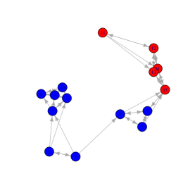
(a)

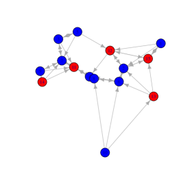
(b)

Figure 1. The directed 3-NN graph on a pooled sample of size 15 in $\mathbb{R}^{2}$ with 10 i.i.d. points from $N(0,\mathrm{I}_{2})$ (colored blue) and 5 i.i.d. points from $N(\Delta\cdot\boldsymbol{1},\mathrm{I}_{2})$ (colored red). For (a) $\Delta=2$, there are 3 directed edges starting from sample 1 and ending in sample 2, and for (b) $\Delta=0.05$, there are 8 such edges.

Another variant is the symmetrized $K$-NN test statistic [29]:

$$T_{S}\bigl{(}\mathcal{N}_{K}\bigl{(}\mathcal{Z}_{N}^{\prime}\bigr{)}\bigr{)}=\sum_{x,y\in\mathcal{Z}_{N}^{\prime}}\psi_{S}(c_{x},c_{y})\boldsymbol{1}\bigl{\{}(x,y)\in E\bigl{(}\mathcal{N}_{K}\bigl{(}\mathcal{Z}_{N}^{\prime}\bigr{)}\bigr{)}\bigr{\}},$$ (1.13)

where $\psi_{S}(c_{x},c_{y})=\bm{1}\{c_{x}\neq c_{y}\}$, which counts the number of (directed) edges with the end-points in the different samples. This can be rewritten as a graph-based test (1.8) by considering the underlying undirected multigraph (which allows for multiple edges between two vertices).

1.4. Summary of results

The asymptotic null distribution and consistency of the tests described above are well known (see [19] for the FR test and [18, 29] for the $K$-NN test). However, a mathematical treatment of the power properties of these tests, which requires understanding the limiting distribution of the test statistics under the alternative, remained unavailable. In this paper, we address this problem by deriving the asymptotic distribution of (1.8), for stabilizing geometric graph functionals, under general alternatives, in the Poissonized setting described above. As a consequence, the exact detection threshold and the limiting local power of these tests can be derived.

We begin with a few notations: For a vector $x\in\mathbb{R}^{p}$, $\|x\|$ and $\|x\|_{1}$ will denote the $L_{2}$ and $L_{1}$ norms of $x$, respectively. For two nonnegative sequences, $(a_{n})_{n\geq 1}$ and $(b_{n})_{n\geq 1}$, $a_{n}=\Theta(b_{n})$ means that there exist positive constants $C_{1},C_{2}$, such that $C_{1}b_{n}\leq a_{n}\leq C_{2}b_{n}$, for all $n$ large enough. Finally, for two positive sequences $(a_{n})_{n\geq 1}$ and $(b_{n})_{n\geq 1}$, we write $a_{n}\ll b_{n}$ or $a_{n}\gg b_{n}$, if $a_{n}/b_{n}\rightarrow 0$ or $a_{n}/b_{n}\rightarrow\infty$, respectively. The results obtained in this paper are summarized below.

1. The limiting distribution of graph-based two-sample tests under general alternatives is derived. The proof of this general result has two main steps: To begin with we show that for tests based on stabilizing geometric graphs, such as the Friedman–Rafsky test (1.11) and the test based on the $K$-nearest-neighbor ($K$-NN) graph (1.12), the statistic (1.8) has a limiting normal distribution, after centering by the conditional mean and scaling by $N^{-\frac{1}{2}}$ (Theorem 3.1). This result is of independent interest, as it leads to a new conditional test, and can be used for approximate power calculations (Remark 3.2). Next, under the stronger assumption of exponential stabilization [24], the conditional CLT can be strengthened to obtain the (unconditional) central limit theorem of (1.8) (Theorem 3.3).

2. The CLT proved above can be used to determine the detection threshold of the $K$-NN test, that is, the rate at which the alternatives shrink toward the null, such that the limiting power of the test transitions from 0 to 1. More precisely, suppose $\{\mathbb{P}_{\theta}\}_{\theta\in\Theta}$ is a parametric family of distributions in $\mathbb{R}^{d}$, indexed by $\theta\in\Theta\subseteq\mathbb{R}^{p}$. Given samples $\mathscr{X}_{N_{1}}^{\prime}$ and $\mathscr{Y}_{N_{2}}^{\prime}$ from $\mathbb{P}_{\theta_{1}}$ and $\mathbb{P}_{\theta_{2}}$ as in (1.5), respectively, consider the testing problem

   $$H_{0}:\theta_{2}-\theta_{1}=0\quad\text{versus}\quad H_{1}:\theta_{2}-\theta_{1}=\varepsilon_{N},$$

   for a sequence $(\varepsilon_{N})_{N\geq 1}$ in $\mathbb{R}^{p}$, such that $\|\varepsilon_{N}\|\rightarrow 0$. The detection threshold for the $K$-NN test is the magnitude of the sequence $\varepsilon_{N}$ below which the test is powerless and above which the test has power going to 1. The parametric rate of detection is $O(N^{-\frac{1}{2}})$; however, results in [6] imply that tests based on geometric graphs, have no power in this scale, that is, they have zero Pitman efficiency, which makes the problem of determining the detection threshold of such tests particularly interesting. In Theorem 4.2, we determine the precise detection threshold of the $K$-NN test, which undergoes a remarkable phase transition at dimension $d\geq 9$, and compute the exact limiting power at the threshold. The result is pictorially represented in Figure 2 and summarized below:

   • For dimension $d\leq 8$, the detection threshold of the test based on the $K$-NN graph (4.3) is at $\Theta(N^{-\frac{1}{4}})$, that is, the limiting power of the test undergoes a phase transition from the level $\alpha$ to 1, depending on whether $\|N^{\frac{1}{4}}\varepsilon_{N}\|\rightarrow 0$ or $\|N^{\frac{1}{4}}\varepsilon_{N}\|\rightarrow\infty$, respectively. Moreover, using the CLT above, we can derive the exact local power at the threshold $N^{\frac{1}{4}}\varepsilon_{N}\rightarrow h$.

   • The detection threshold changes for dimension $d\geq 9$, where the situation becomes more delicate: Here, the $K$-NN test has power going to $\alpha$ or 1, depending on whether $\|N^{\frac{1}{2}-\frac{2}{d}}\varepsilon_{N}\|\rightarrow 0$ or $\|N^{\frac{2}{d}}\varepsilon_{N}\|\rightarrow\infty$, respectively. This shows that the detection threshold is somewhere between these two bounds, however, unlike in $d\leq 8$, the exact location of the detection threshold has no universality: it depends on the distribution of the data under the null and the direction along which $\varepsilon_{N}$ goes to zero. Note that the exponent in the lower bound $\frac{1}{2}-\frac{2}{d}$ increases to $\frac{1}{2}$ (the parametric detection threshold), and the exponent in the upper bound decreases to the 0 (which gives consistent fixed alternatives). We show that both these thresholds are tight in a truncated spherical normal problem, depending on the sign of the alternative. This is an example where the $K$-NN test exhibit a surprising blessing of dimensionality, that is, it becomes easier to detect local changes along certain directions as dimension increases (see Section 4.2.2 for details). The reason behind the phase transition of the detection threshold at dimension 9 is explained in Section 4.1.1, and the details of the proof are given in Appendix B.

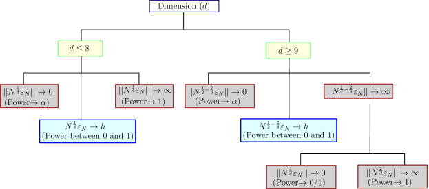
Figure 2. Detection threshold of the test based on the $K$-NN graph: Illustration of Theorem 4.2.

1.5. Organization

The rest of the paper is organized as follows: The general consistency result is stated in Section 2. The central limit theorems for the statistic (1.8) are described in Section 3. The detection threshold and local power of the $K$-NN test are given in Section 4.1, and the performance of the different tests are compared in simulations in Section 4.2. The proofs of the results are given in the Appendix.

2. Consistency

In this section, we prove consistency against all fixed alternatives of the test (1.9) for stabilizing graphs functionals. This unifies the proof of consistency of the test based on the $K$-NN graph [29, 18], and the FR test [19], generalizing the result to any stabilizing graph. We begin by recalling that $d(x,\mathscr{G}(S))$ is the total degree of the vertex $x$ in $\mathscr{G}(S\cup\{x\})$, for $S\subset\mathbb{R}^{d}$ nice and $x\in\mathbb{R}^{d}$. Moreover, for a function $\psi:\mathbb{R}^{d}\rightarrow\mathbb{R}$, we denote by $\mathcal{P}_{\psi}$ the inhomogeneous Poisson process with intensity function $\psi$. (In particular, this means for any measurable set $A\subset\mathbb{R}^{d}$, the number of points in $A$ is distributed as $\operatorname{Pois}(\int_{A}\psi(x)\,\mathrm{d}x)$.)

Assumption 2.1 (Degree moment condition).

A translation and scale invariant graph functional $\mathscr{G}$ is said to satisfy the $\beta$-degree moment condition if it stabilizes on $\mathcal{P}_{\lambda}$, for all $\lambda\in(0,\infty)$, and

$$\sup_{N\in\mathbb{N}}\sup_{\begin{subarray}{c}z\in\mathbb{R}^{d},\\ \mathcal{A}\subset\mathbb{R}^{d}\end{subarray}}\mathbb{E}\bigl{\{}d^{\beta}\bigl{(}z,\mathscr{G}(\mathcal{P}_{N\phi_{N}}\cup\mathcal{A})\bigr{)}\bigr{\}}<\infty,$$ (2.1)

where $\mathcal{A}$ ranges over all finite subsets of $\mathbb{R}^{d}$, and $\phi_{N}=\frac{N_{1}}{N}f+\frac{N_{2}}{N}g$.

This condition ensures that the $\beta$-th moment of the degree function at a point $z$ is uniformly bounded over $z$ and over the addition of finitely many points to the data. Note that this is trivially satisfied for bounded degree graphs, such as the $K$-NN and the MST. Under this assumption, the weak limit of the statistic $\frac{1}{N}T(\mathscr{G}(\mathcal{Z}_{N}^{\prime}))$ can be derived, which is given in terms of the Henze–Penrose dissimilarity measure between the two density functions.

Definition 2.1.

Given $p\in(0,1)$ and densities $f$ and $g$ in $\mathbb{R}^{d}$, the Henze–Penrose dissimilarity measure is defined as

$$\delta(f,g,p)=1-2pq\int\frac{f(x)g(x)}{pf(x)+qg(x)}\,\mathrm{d}x.$$ (2.2)

This belongs to a general class of separation measures between probability distributions [16].

The following proposition gives the weak-limit of $\frac{1}{N}T(\mathscr{G}(\mathcal{Z}_{N}^{\prime}))$ for stabilizing graph functionals satisfying the degree moment condition. The proof of the proposition closely mimics [19], Theorem 2, and is detailed in Section A.3.

Proposition 2.1.

Let $\mathscr{G}$ be a translation and scale invariant directed graph functional which stabilizes on $\mathcal{P}_{\lambda}$ for all $\lambda\in(0,\infty)$. If $\mathscr{G}$ satisfies the $\beta$-degree moment condition for some $\beta>4$, then

$$\frac{1}{N}T\bigl{(}\mathscr{G}\bigl{(}\mathcal{Z}_{N}^{\prime}\bigr{)}\bigr{)}\stackrel{{\scriptstyle P}}{{\to}}\frac{\mathbb{E}\Delta_{0}^{\uparrow}}{2}\bigl{(}1-\delta(f,g,p)\bigr{)},$$ (2.3)

where $\Delta_{0}^{\uparrow}=d^{\uparrow}(0,\mathscr{G}(\mathcal{P}_{1}))$ is the out-degree of the origin in the graph $\mathscr{G}(\mathcal{P}_{1}\cup\{0\})$.

Using the fact $\delta(f,g,p)\geq\delta(f,f,p)=p^{2}+q^{2}$ and that the inequality is strict for densities $f$ and $g$ differing on a set of positive measure (see [16], Theorem 1 and Corollary 1), it can be shown that various tests based on stabilizing graph functionals, which includes the MST and the $K$-NN graphs, are consistent for all fixed alternatives (1.2) (refer to Remark A.2 for details).

Remark 2.1.

Recently, Arias-Castro and Pelletier [2] showed that Rosenbaum’s cross match test [26] based on non-bipartite matching (NBM), has the same limit as in (2.3), thus it is also consistent for general alternatives. Note that this does not follow from Proposition 2.1, because it is unknown whether the NBM graph functional is stabilizing. They show that the properties of stabilizing graphs required in the proof of consistency also hold for the NBM graph functional and, therefore, (2.3) holds for the cross match test as well.

3. Distribution under general alternatives

This section describes the central limit theorems of the Poissonized two sample statistic $T(\mathscr{G}(\mathcal{Z}_{N}^{\prime}))$ (recall (1.8)) for stabilizing graph functionals. Let $\mathscr{X}_{N_{1}}^{\prime}$ and $\mathscr{Y}_{N_{2}}^{\prime}$ be Poissonized samples from densities $f$ and $g$ in $\mathbb{R}^{d}$ as in (1.5). Define

$$\phi_{N}(x)=\frac{N_{1}}{N}f(x)+\frac{N_{2}}{N}g(x)\quad\text{and}\quad\phi(x)=pf(x)+qg(x).$$ (3.1)

Recall from Section 1.2 that the joint distribution of $\mathscr{X}_{N_{1}}^{\prime}$ and $\mathscr{Y}_{N_{2}}^{\prime}$ can be described as follows: Let $\mathcal{Z}^{\prime}=\{Z_{1},Z_{2},\ldots\}$ be independent random variables with common density $\phi_{N}$. Then $\mathcal{Z}_{N}^{\prime}=\{Z_{1},Z_{2},\ldots,Z_{L_{N}}\}$, where $L_{N}\sim\operatorname{Pois}(N)$ is independent of $\mathcal{Z}^{\prime}$, and each point of $\mathcal{Z}_{N}^{\prime}$ is labeled 1 or 2 as in (1.7). Then the sets of points assigned labels 1 and 2 have the same distribution as $\mathscr{X}_{N_{1}}^{\prime}$ and $\mathscr{Y}_{N_{2}}^{\prime}$. In this section, we derive the limiting distribution of the test statistic

$$\mathcal{R}\bigl{(}\mathscr{G}\bigl{(}\mathcal{Z}_{N}^{\prime}\bigr{)}\bigr{)} =\frac{1}{\sqrt{N}}\bigl{\{}T\bigl{(}\mathscr{G}\bigl{(}\mathcal{Z}_{N}^{\prime}\bigr{)}\bigr{)}-\mathbb{E}_{H_{1}}\bigl{(}T\bigl{(}\mathscr{G}\bigl{(}\mathcal{Z}_{N}^{\prime}\bigr{)}\bigr{)}\bigr{)}\bigr{\}}$$ (3.2)

for stabilizing graph functionals. This involves the following two steps:

1. The first step is to derive the CLT of the test statistic centered by the conditional mean $\mathbb{E}_{H_{1}}(T(\mathscr{G}(\mathcal{Z}_{N}^{\prime}))|\mathcal{F})$, where $\mathcal{F}:=\sigma(\mathcal{Z}^{\prime},L_{N})$ is the sigma-algebra generated by $\mathcal{Z}^{\prime}$ and the Poisson random variable $L_{N}$, that is,

   $$\mathcal{R}_{1}\bigl{(}\mathscr{G}\bigl{(}\mathcal{Z}_{N}^{\prime}\bigr{)}\bigr{)}=\frac{1}{\sqrt{N}}\bigl{\{}T\bigl{(}\mathscr{G}\bigl{(}\mathcal{Z}_{N}^{\prime}\bigr{)}\bigr{)}-\mathbb{E}_{H_{1}}\bigl{(}T\bigl{(}\mathscr{G}\bigl{(}\mathcal{Z}_{N}^{\prime}\bigr{)}\bigr{)}|\mathcal{F}\bigr{)}\bigr{\}},$$ (3.3)

   for a stabilizing graph functional $\mathscr{G}$. Note that conditional on $\mathcal{F}$, the randomness comes from the labeling (1.7). As the labeling is independent across the vertices of the graph, the dependence in (3.3) is local, and the CLT can be proved using Stein’s method based on dependency graphs (Theorem 3.1). This can be used to devise and calibrate a conditional test (see Remark 3.2), which might be of independent interest.

2. The second step is to derive the CLT of the conditional mean

   $$\mathcal{R}_{2}\bigl{(}\mathscr{G}\bigl{(}\mathcal{Z}_{N}^{\prime}\bigr{)}\bigr{)}=\frac{1}{\sqrt{N}}\bigl{\{}\mathbb{E}_{H_{1}}\bigl{(}T\bigl{(}\mathscr{G}\bigl{(}\mathcal{Z}_{N}^{\prime}\bigr{)}\bigr{)}|\mathcal{F}\bigr{)}-\mathbb{E}_{H_{1}}\bigl{(}T\bigl{(}\mathscr{G}\bigl{(}\mathcal{Z}_{N}^{\prime}\bigr{)}\bigr{)}\bigr{)}\bigr{\}}.$$ (3.4)

   This requires the additional assumption of exponential stabilization (Definition 3.2), and is proved in Proposition 3.2.

The above results can be combined to obtain the CLT of (3.2), since $\mathcal{R}(\mathscr{G}(\mathcal{Z}_{N}^{\prime}))=\mathcal{R}_{1}(\mathscr{G}(\mathcal{Z}_{N}^{\prime}))+\mathcal{R}_{2}(\mathscr{G}(\mathcal{Z}_{N}^{\prime}))$ (see Theorem 3.3 below for details).

3.1. The conditional CLT

For a directed graph functional $\mathscr{G}$, $S\subset\mathbb{R}^{d}$ finite and a point $x\in\mathbb{R}^{d}$, let $d^{\uparrow}(x,\mathscr{G}(S))$ be the out-degree of the vertex $x$ in the graph $\mathscr{G}(S\cup\{x\})$, that is, the number of outgoing edges $(x,y)$, where $y\in S\cup\{x\}$, in the graph $\mathscr{G}(S\cup\{x\})$. Similarly, let $d^{\downarrow}(x,\mathscr{G}(S))$ be the in-degree of the vertex $x$ in the graph $\mathscr{G}(S\cup\{x\})$, that is, the number of incoming edges $(y,x)$, where $y\in S\cup\{x\}$, in the graph $\mathscr{G}(S\cup\{x\})$. Note that $d(x,\mathscr{G}(S))=d^{\downarrow}(x,\mathscr{G}(S))+d^{\uparrow}(x,\mathscr{G}(S))$ is the total degree of the vertex $x$ in the graph $\mathscr{G}(S\cup\{x\})$.

Moreover, let

$$T_{2}^{\uparrow}\bigl{(}x,\mathscr{G}(S)\bigr{)}={d^{\uparrow}\bigl{(}x,\mathscr{G}(S)\bigr{)}\choose 2},\qquad T_{2}^{\downarrow}\bigl{(}x,\mathscr{G}(S)\bigr{)}={d^{\downarrow}\bigl{(}x,\mathscr{G}(S)\bigr{)}\choose 2}$$ (3.5)

be the number of outward 2-stars and inward 2-stars incident on $x$ in $\mathscr{G}(S)$, respectively. Finally, let $T_{2}^{+}(x,\mathscr{G}(S))$ be the number of 2-stars incident on $x$ in $\mathscr{G}(S)$ with different directions on the two edges. For notational brevity, denote

$$\Delta^{\uparrow}_{0}=d^{\uparrow}\bigl{(}0,\mathscr{G}(\mathcal{P}_{1})\bigr{)},\qquad\Delta^{\downarrow}_{0}=d^{\downarrow}\bigl{(}0,\mathscr{G}(\mathcal{P}_{1})\bigr{)},$$ (3.6)

and $\Delta^{+}_{0}:=|\{z\in\mathcal{P}_{1}:(0,z),(z,0)\in E(\mathscr{G}(\mathcal{P}_{1}^{0}))\}|$. (Note that $\Delta^{\uparrow}_{0}$ was already defined in the statement of Proposition 2.1.) Similarly, let

$$T_{2}^{\uparrow}=T_{2}^{\uparrow}\bigl{(}0,\mathscr{G}(\mathcal{P}_{1})\bigr{)},\qquad T_{2}^{\downarrow}=T_{2}^{\downarrow}\bigl{(}0,\mathscr{G}(\mathcal{P}_{1})\bigr{)},$$ (3.7)

and $T_{2}^{+}:=T_{2}^{+}(0,\mathscr{G}(\mathcal{P}_{1}))$.

To derive the CLT of (3.3), we need some control on the maximum degree of the graph functional $\mathscr{G}$. The natural assumption of bounded maximum degree includes most of the natural graphs, such as the MST and the $K$-NN graph. The slightly weaker polynomial upper bound given below includes other stabilizing geometric graphs, like the Delaunay graph [25].

Assumption 3.1 (Maximum degree condition).

A graph functional $\mathscr{G}$ is said to satisfy the maximum degree condition if

$$\sup_{z\in\mathcal{P}_{N\phi_{N}}}d\bigl{(}z,\mathscr{G}(\mathcal{P}_{N\phi_{N}})\bigr{)}=o_{P}\bigl{(}N^{\frac{1}{40}}\bigr{)}.$$ (3.8)

The following theorem gives the CLT of the test statistic centered by the conditional mean, as in (3.3), for stabilizing graph functionals. Recall $\phi(x)=pf(x)+qg(x)$.

Theorem 3.1.

Let $\mathscr{G}$ be a translation and scale invariant directed graph functional which stabilizes on $\mathcal{P}_{\lambda}$, for all $\lambda\in(0,\infty)$. If $\mathscr{G}$ satisfies the $\beta$-degree moment condition for $\beta>4$ and the maximum degree condition (3.8), then

$$\mathcal{R}_{1}\bigl{(}\mathscr{G}\bigl{(}\mathcal{Z}_{N}^{\prime}\bigr{)}\bigr{)}\stackrel{{\scriptstyle D}}{{\to}}N\bigl{(}0,\kappa_{\mathscr{G}}^{2}\bigr{)},$$

where

$$\kappa_{\mathscr{G}}^{2}=\frac{r}{4}\int\frac{f(x)g(x)}{\phi^{3}(x)}L(x)\,\mathrm{d}x,$$ (3.9)

with $r:=2pq$, and

$$L(x):=2\mathbb{E}\Delta_{0}^{\uparrow}\phi^{2}(x)+4\phi(x)\bigl{(}q\mathbb{E}T_{2}^{\uparrow}g(x)+p\mathbb{E}T_{2}^{\downarrow}f(x)\bigr{)}-4pq\mathbb{E}\Gamma_{0}f(x)g(x),$$

where $\Gamma_{0}:=T_{2}^{\uparrow}+T_{2}^{\downarrow}+T_{2}^{+}+\frac{\Delta^{+}_{0}}{2}+\frac{\Delta_{0}^{\uparrow}}{2}$, with $\Delta_{0}^{\uparrow}$, $\Delta_{0}^{\downarrow}$, $T_{2}^{\uparrow}$, and $T_{2}^{\downarrow}$ as defined in (3.6) and (3.7).

The proof of theorem is given in Section A.4. The limit of the conditional variance (3.9) is derived using properties of stabilizing graphs, and the CLT is proved using Stein’s method based on dependency graphs. In fact, our proof suggests that it is possible to extend the CLT in Theorem 3.1 to other distance functions in $\mathbb{R}^{d}$, whenever the maximum degree condition (Assumption 3.1) holds, and the conditional variance of $\mathcal{R}_{1}(\mathscr{G}(\mathcal{Z}_{N}^{\prime}))$ has a limit in probability, in the graph $\mathscr{G}(\mathcal{Z}_{N}^{\prime})$ constructed using that metric. This is because our proof technique proceeds by conditioning on the randomness of the graph and, therefore, as long as the associated graph quantities that arise in $\operatorname{Var}(\mathcal{R}_{1}(\mathscr{G}(\mathcal{Z}_{N}^{\prime}))|\mathcal{F})$ converge in probability (as in Lemma A.5), and the dependence is local (which is ensured by Assumption 3.1), the Stein’s method argument applies and the asymptotic normality in Theorem 3.1 would hold.

Remark 3.1 (Null distribution).

Given the graph functional $\mathscr{G}$, the limit of the conditional variance $\kappa_{\mathscr{G}}$ depends on the densities $f$ and $g$ and the limiting proportion $p$ of the samples. Under the null ($f=g$) this simplifies to

$$\kappa_{\mathscr{G},H_{0}}^{2}=\frac{r}{4}\bigl{\{}2\mathbb{E}\Delta_{0}^{\uparrow}+4\bigl{(}q\mathbb{E}T_{2}^{\uparrow}+p\mathbb{E}T_{2}^{\downarrow}\bigr{)}-2r\Gamma_{0}\bigr{\}}.$$ (3.10)

• $\mathscr{G}=\mathcal{N}_{K}$ is the $K$-NN nearest neighbor graph functional: In this case, $\Delta_{0}^{\uparrow}=K$, $T_{2}^{\uparrow}=\frac{K(K-1)}{2}$, $T_{2}^{+}=\Delta_{0}^{\uparrow}\Delta_{0}^{\downarrow}-\Delta_{0}^{+}=K\Delta_{0}^{\downarrow}-\Delta_{0}^{+}$, $\mathbb{E}\Delta^{\downarrow}=K$, and (3.10) simplifies to

  $$\kappa_{\mathcal{N}_{K},H_{0}}^{2} =\frac{r}{2}\bigl{\{}Kpq+(p-q)^{2}K^{2}+p^{2}\operatorname{Var}\bigl{(}\Delta_{0}^{\downarrow}\bigr{)}+pq\mathbb{E}\Delta_{0}^{+}\bigr{\}}.$$ (3.11)

• $\mathscr{G}$ is an undirected graph functional: In this case (3.10) simplifies to

  $$\kappa_{\mathscr{G},H_{0}}^{2}=\frac{r}{2}\bigl{\{}r\mathbb{E}\Delta_{0}+\mathbb{E}\bigl{(}\Delta_{0}^{2}\bigr{)}(1-2r)\bigr{\}},$$ (3.12)

  since $\mathbb{E}T_{2}^{\uparrow}=\mathbb{E}T_{2}^{\downarrow}=\mathbb{E}\frac{\Delta_{0}(\Delta_{0}-1)}{2}$, $\mathbb{E}T_{2}^{+}=\mathbb{E}\Delta_{0}(\Delta_{0}-1)$ and $\mathbb{E}\Delta_{0}^{+}=\mathbb{E}\Delta_{0}$. For example, when $\mathscr{G}=\mathcal{T}$ is the MST graph functional as in the Friedman–Rafsky test (1.11), $\Delta_{0}=2$ ([1], Lemma 7), and (3.12) becomes $\kappa_{\mathcal{T},H_{0}}^{2}=r\{r+\frac{1}{2}\mathbb{E}(\Delta_{0}^{2})(1-2r)\}$.

The above discussion suggests that the CLT in Theorem 3.1 can be used to derive a conditional test for (1.2).

Remark 3.2 (A conditional test and its power).

For concreteness, suppose $\mathscr{G}=\mathcal{T}$ is the MST. Then under the null $\mathbb{E}_{H_{0}}(T(\mathcal{T}(\mathcal{Z}_{N}^{\prime}))|\mathcal{F})=\frac{N_{1}N_{2}}{(N_{1}+N_{2})^{2}}$ $|E(\mathcal{T}(\mathcal{Z}_{N}^{\prime}))|=\frac{N_{1}N_{2}}{(N_{1}+N_{2})^{2}}(L_{N}-1)$, and given the data, we reject $H_{0}$ whenever

$$\frac{1}{\sqrt{N}}\biggl{\{}T\bigl{(}\mathcal{T}\bigl{(}\mathcal{Z}_{N}^{\prime}\bigr{)}\bigr{)}-\frac{N_{1}N_{2}}{(N_{1}+N_{2})^{2}}L_{N}\biggr{\}}\leq\kappa_{\mathscr{G},H_{0}}z_{\alpha}.$$

By Theorem 3.1, this test has asymptotically level $\alpha$. Moreover, it can be shown that (see Section A.3 for details) that

$$\mathbb{E}_{H_{1}}\bigl{(}T\bigl{(}\mathscr{G}\bigl{(}\mathcal{Z}_{N}^{\prime}\bigr{)}\bigr{)}|\mathcal{F}\bigr{)}=\sum_{1\leq i\neq j\leq L_{N}}\frac{N_{1}N_{2}f(Z_{i})g(Z_{j})\bm{1}\{(Z_{i},Z_{j})\in E(\mathscr{G}(\mathcal{Z}_{N}^{\prime}))\}}{(N_{1}f(Z_{i})+N_{2}g(Z_{j}))(N_{1}f(Z_{i})+N_{2}g(Z_{j}))}.$$

The proof of Proposition 2.1 reveals that this test is consistent against all fixed alternatives, and using Theorem 3.1 we can compute the approximate power of this test as

$$\Phi\biggl{(}\frac{\kappa_{\mathscr{G},H_{0}}z_{\alpha}-\Xi(\mathcal{Z}_{N}^{\prime})}{\kappa_{\mathscr{G}}}\biggr{)},$$ (3.13)

where $\Xi(\mathcal{Z}_{N}^{\prime})=\frac{1}{\sqrt{N}}(\mathbb{E}_{H_{1}}(T(\mathscr{G}(\mathcal{Z}_{N}^{\prime}))|\mathcal{F})-\mathbb{E}_{H_{0}}(T(\mathscr{G}(\mathcal{Z}_{N}^{\prime}))|\mathcal{F}))$ is the difference of the conditional means under the alternative and the null, which can be calculated from the data. The approximation in (3.13) can be justified because Stein’s method gives uniform control on the corresponding distribution functions (see Proposition A.2 in the Appendix). (Note that the argument above holds for any stabilizing graph functional, as long as the number of edges $|E(\mathscr{G}(\mathcal{Z}_{N}^{\prime}))|$ does not depend on the unknown null distribution, as is the case for the Friedman–Rafsky test and the test based on the $K$-NN graph.)

3.2. CLT of the test statistic under general alternatives

In this section, the (unconditional) CLT of the test statistic (3.2) is derived. This involves finding the CLT of the conditional mean (3.4), which requires the stronger notion of exponential stabilization [24]. For any locally finite point set $\mathcal{H}\subset\mathbb{R}^{d}$ and $x\in\mathbb{R}^{d}$, define the out-degree measure of a graph functional $\mathscr{G}$ as follows: For all Borel sets $A\subset\mathbb{R}^{d}$,

$$d_{\mathscr{G}}^{\uparrow}(x,\mathcal{H},A)=\sum_{y\in\mathcal{H}^{x}\cap A}\bm{1}\bigl{\{}(x,y)\in E\bigl{(}\mathscr{G}\bigl{(}\mathcal{H}^{x}\bigr{)}\bigr{)}\bigr{\}},$$ (3.14)

where $\mathcal{H}^{x}=\mathcal{H}\cup\{x\}$. In other words, the out-degree measure of a set $A$, with respect to $\mathcal{H}$ and $x$ is the number of edges incident on $x$ with the other end point in $\mathcal{H}^{x}\cap A$ in the graph $\mathscr{G}(\mathcal{H}^{x})$. The following definition formalizes the notion of “radius of stabilization” of a point, which is the smallest radius outside which addition of finitely many points does not affect the degree measure at the point.

Definition 3.1.

Fix a locally finite point set $\mathcal{H}$, a point $x\in\mathbb{R}^{d}$, and a Borel set $A\subseteq\mathbb{R}^{d}$. The radius of stabilization of the degree measure (3.14) at $x$ with respect to $\mathcal{H}$ and $A$ (to be denoted by $R(x,\mathcal{H},A)$) is the smallest $R\geq 0$ such that

$$d_{\mathscr{G}}^{\uparrow}\bigl{(}x,x+\bigl{\{}\mathcal{H}\cap B(0,R)\cup\mathcal{Y}\bigr{\}},x+B\bigr{)}=d_{\mathscr{G}}^{\uparrow}\bigl{(}x,x+\bigl{\{}\mathcal{H}\cap B(0,R)\bigr{\}},x+B\bigr{)},$$ (3.15)

for all finite $\mathcal{Y}\subseteq A\backslash B(0,R)$ and all Borel subsets $B\subseteq A$, where $B(0,R)$ is the (Euclidean) ball of radius $R$ with center at the point $0\in\mathbb{R}^{d}$. If no such $R$ exists, then set $R(x,\mathcal{H},A)=\infty$.

Throughout this section, we will assume that $f$ and $g$ have a common support $S$, which is compact and convex, and $N\rightarrow\infty$ such that

$$\sqrt{N}\biggl{(}\frac{N_{1}}{N_{1}+N_{2}}-p\biggr{)}\rightarrow 0\quad\text{and}\quad\sqrt{N}\biggl{(}\frac{N_{1}}{N_{1}+N_{2}}-q\biggr{)}\rightarrow 0.$$ (3.16)

Definition 3.2.

Let $R_{N}(x):=R(x,\mathcal{P}_{N\phi_{N}},S)$ be the radius of stabilization of out-degree measure $d_{\mathscr{G}}^{\uparrow}$ at $x$ with respect to the Poisson process $\mathcal{P}_{N\phi_{N}}$ and $S$. Define

$$\tau(s):=\sup_{N\in\mathbb{N}}\sup_{x\in\mathbb{R}^{d}}\mathbb{P}\bigl{(}R_{N\phi_{N}}(x)>N^{-\frac{1}{d}}s\bigr{)}.$$ (3.17)

The out-degree measure $d_{\mathscr{G}}^{\uparrow}$ is said to be

• power law stabilizing of order $q$ if $\sup_{s\geq 1}s^{q}\tau(s)<\infty$,

• exponentially stabilizing if $\lim\sup_{s\rightarrow\infty}\frac{1}{s}\log\tau(s)<0$.

Conditions on the decay of the tail of the radius of stabilization, similar to (3.17) above, is a standard requirement for proving limit theorems of functionals of random geometric graphs [24, 34]. Using this machinery, we prove the following theorem, which gives the CLT of the conditional mean (3.4) for exponentially stabilizing random geometric graphs.

Proposition 3.2.

Let $\mathscr{G}$ be a translation and scale invariant directed graph functional in $\mathbb{R}^{d}$ which satisfies the $\beta$-degree moment condition (2.1) for some $\beta>2$. If the out-degree measure $d_{\mathscr{G}}^{\uparrow}$ is power law stabilizing of order $q>\frac{\beta}{\beta-2}$, then

$$\lim_{N\rightarrow\infty}\operatorname{Var}\bigl{(}\mathcal{R}_{2}\bigl{(}\mathscr{G}\bigl{(}\mathcal{Z}_{N}^{\prime}\bigr{)}\bigr{)}\bigr{)}=\tau_{\mathscr{G}}^{2},$$ (3.18)

where

$$\tau_{\mathscr{G}}^{2}=\frac{r^{2}}{4}L_{0}\int\frac{f^{2}(x)g^{2}(x)}{\phi^{3}(x)}\,\mathrm{d}x,$$ (3.19)

where $L_{0}:=\int(\mathbb{E}\{d^{\uparrow}(0,\mathscr{G}(\mathcal{P}_{1}^{z}))d^{\uparrow}(z,\mathscr{G}(\mathcal{P}_{1}^{0}))\}-(\mathbb{E}\Delta_{0}^{\uparrow})^{2})\,\mathrm{d}z+\mathbb{E}(\Delta_{0}^{\uparrow})^{2}$. Moreover, if $d_{\mathscr{G}}^{\uparrow}$ is exponentially stabilizing then $\mathcal{R}_{2}(\mathscr{G}(\mathcal{Z}_{N}^{\prime}))\stackrel{{\scriptstyle D}}{{\to}}N(0,\tau_{\mathscr{G}}^{2})$.

The proof of theorem is given in Section A.6.1. Combining Theorem 3.1 and Proposition 3.2, the CLT of $\mathcal{R}(\mathscr{G}(\mathcal{Z}_{N}^{\prime}))$ (defined in (3.2)) can be obtained. The proof is in Section A.6.2.

Theorem 3.3.

Let $\mathscr{G}$ be a translation and scale invariant directed graph functional which satisfies the $\beta$-degree moment condition for some $\beta>4$ and the maximum out-degree condition (3.8). If the degree measure $d_{\mathscr{G}}^{\uparrow}$ is exponentially stabilizing, then

$$\mathcal{R}\bigl{(}\mathscr{G}\bigl{(}\mathcal{Z}_{N}^{\prime}\bigr{)}\bigr{)}\stackrel{{\scriptstyle D}}{{\to}}N\bigl{(}0,\sigma^{2}_{\mathscr{G}}\bigr{)},$$ (3.20)

where $\sigma^{2}_{\mathscr{G}}=\kappa_{\mathscr{G}}^{2}+\tau_{\mathscr{G}}^{2}$, with $\kappa_{\mathscr{G}}^{2}$ and $\tau_{\mathscr{G}}^{2}$ as defined in (3.9) and (3.19), respectively.

Many random geometric graphs, such as the $K$-NN graph and the Delaunay graph [24, 25] are exponentially stabilizing. This theorem gives the asymptotic distribution of two-sample tests based on such graphs, under general alternatives. This can be used to the compute power of such tests as in Remark 3.2. Moreover, using this we can understand the asymptotic performances of the tests, by identifying testable local alternatives, as elaborated in the following section for the test based on the $K$-NN graph. The techniques used in this section might also be useful in studying limiting distributions of multivariate goodness-of-fit tests based on nearest neighbors [7, 13].

To see why the asymptotic variance in (3.20) is the sum of two terms, note that

$$\operatorname{Var}\bigl{(}\mathcal{R}\bigl{(}\mathscr{G}\bigl{(}\mathcal{Z}_{N}^{\prime}\bigr{)}\bigr{)}\bigr{)} =\mathbb{E}\bigl{(}\operatorname{Var}\bigl{(}\mathcal{R}\bigl{(}\mathscr{G}\bigl{(}\mathcal{Z}_{N}^{\prime}\bigr{)}\bigr{)}|\mathcal{F}\bigr{)}\bigr{)}+\operatorname{Var}\bigl{(}\mathbb{E}\bigl{(}\mathcal{R}\bigl{(}\mathscr{G}\bigl{(}\mathcal{Z}_{N}^{\prime}\bigr{)}\bigr{)}|\mathcal{F}\bigr{)}\bigr{)},$$

where $\mathcal{F}:=\sigma(\mathcal{Z}^{\prime},L_{N})$ is the sigma-algebra generated by $\mathcal{Z}^{\prime}$ and the Poisson random variable $L_{N}$ (recall notation from Section 1.2). Now, recalling (3.3) shows $\operatorname{Var}(\mathcal{R}(\mathscr{G}(\mathcal{Z}_{N}^{\prime}))|\mathcal{F})=\operatorname{Var}(\mathcal{R}_{1}(\mathscr{G}(\mathcal{Z}_{N}^{\prime}))|\mathcal{F})$, and (3.4) gives $\operatorname{Var}(\mathbb{E}(\mathcal{R}(\mathscr{G}(\mathcal{Z}_{N}^{\prime}))|\mathcal{F}))=\operatorname{Var}(\mathcal{R}_{2}(\mathscr{G}(\mathcal{Z}_{N}^{\prime})))$. In the proof of Theorem 3.1, we show that $\operatorname{Var}(\mathcal{R}_{1}(\mathscr{G}(\mathcal{Z}_{N}^{\prime}))|\mathcal{F})$ converges in $L_{2}$ to $\kappa_{\mathscr{G}}^{2}$ (Lemma A.5), while the proof of Proposition 3.2 shows that $\operatorname{Var}(\mathcal{R}_{2}(\mathscr{G}(\mathcal{Z}_{N}^{\prime})))\rightarrow\tau_{\mathscr{G}}^{2}$ (Section A.6.1), hence the asymptotic variance in (3.20) is the sum of these two terms.

Remark 3.3.

(Comments on de-Poissonization) Poissionization is a commonly used trick in geometric probability, where calculations become simpler because of the spatial independence of the Poisson process. In fact, when the sample sizes are large, one can pretend that the data comes from Poissonized samples with a slightly smaller mean, since a Poisson random variable is tightly concentrated around its expectation. De-Poissionization techniques are well known ([23], Section 2.5 and [24], Theorem 2.3), using which one can expect to de-Poissonize the CLT in Theorem 3.3 for the test based on the $K$-NN graph. The only thing that would change is the formula of the asymptotic variance, but its derivation is quite tedious for general alternatives. However, for the implementation of the test, we are more interested in the asymptotic null variance, where the calculations are much simpler, and the de-Poissonized null variance can be easily computed (see Section A.5). In fact, de-Poissonization would only change the asymptotic variance (not the order), and the constants in the limiting power (but, not the rates). Therefore, de-Poissonization would not affect (most of) the results of Section 4 as these mainly focus on detection thresholds. This is also validated by the simulations in Section 4.2.

4. Local power of the $K$-NN test

The test based on the $K$-NN graph is exponentially stabilizing and, therefore, the results obtained in the previous section apply. Recall that we assume $f$, $g$ have a common support $S$ which is compact and convex, and $N\rightarrow\infty$ such that (3.16) hold. Then we have the following corollary of Theorem 3.3.

Corollary 4.1.

For the $K$-NN graph functional $\mathcal{N}_{K}$ and $f$ and $g$ as above:

$$\mathcal{R}\bigl{(}\mathcal{N}_{K}\bigl{(}\mathcal{Z}_{N}^{\prime}\bigr{)}\bigr{)}\stackrel{{\scriptstyle D}}{{\to}}N\bigl{(}0,\sigma^{2}_{\mathcal{N}_{K}}\bigr{)},$$ (4.1)

where $\sigma^{2}_{\mathcal{N}_{K}}=\kappa_{\mathcal{N}_{K}}^{2}+\frac{r^{2}K^{2}}{4}\int\frac{f^{2}(x)g^{2}(x)}{\phi^{3}(x)}\,\mathrm{d}x$, with $\kappa_{\mathcal{N}_{K}}$ as defined in (3.9).

Proof.

Note that the graph functional $\mathcal{N}_{K}$ is exponentially stabilizing [24] and satisfies the degree moment condition for $\beta>4$. Therefore, by Theorem 3.3, (4.1) holds with $\sigma^{2}_{\mathcal{N}_{K}}=\kappa_{\mathcal{N}_{K}}^{2}+\tau_{\mathcal{N}_{K}}^{2}$. The result follows by noting that $\tau_{\mathcal{N}_{K}}^{2}=\frac{r^{2}K^{2}}{4}\int\frac{f^{2}(x)g^{2}(x)}{\phi^{3}(x)}\,\mathrm{d}x$ (recall (3.19)). ∎

Remark 4.1.

Under the null $(f=g)$, $\tau_{\mathcal{N}_{K},H_{0}}^{2}=\frac{r^{2}K^{2}}{4}$, and using (3.11), the asymptotic variance (4.1) simplifies to

$$\begin{split}\sigma_{K}^{2}&:=\sigma^{2}_{\mathcal{N}_{K},H_{0}}=\kappa_{\mathcal{N}_{K},H_{0}}^{2}+\tau_{\mathcal{N}_{K},H_{0}}^{2}\\ &=\frac{r}{2}\bigl{\{}K(K+1)pq+(p-q)^{2}K^{2}+p^{2}\operatorname{Var}\bigl{(}\Delta_{0}^{\downarrow}\bigr{)}\bigr{\}}.\end{split}$$ (4.2)

Then recalling (1.9), the two-sample test based on $\mathcal{N}_{K}$ rejects when

$$\frac{1}{\sqrt{N}}\bigl{\{}T\bigl{(}\mathcal{N}_{K}\bigl{(}\mathcal{Z}_{N}^{\prime}\bigr{)}\bigr{)}-\mathbb{E}_{H_{0}}\bigl{(}T\bigl{(}\mathcal{N}_{K}\bigl{(}\mathcal{Z}_{N}^{\prime}\bigr{)}\bigr{)}\bigr{)}\bigr{\}}\leq\sigma_{K}z_{\alpha}.$$ (4.3)

4.1. Power against local alternatives

In this section, we determine the power of the $K$-NN test against local alternatives, that is, the power when the alternatives shrink (with increasing sample size) toward the null at a certain rate. To this end, let $\Theta\subseteq\mathbb{R}^{p}$ be the parameter space and $\{\mathbb{P}_{\theta}\}_{\theta\in\Theta}$ be a parametric family of distributions in $\mathbb{R}^{d}$ with density $f(\cdot|\theta)$. Let $\mathscr{X}_{N_{1}}^{\prime}$ and $\mathscr{Y}_{N_{2}}^{\prime}$ be samples from $\mathbb{P}_{\theta_{1}}$ and $\mathbb{P}_{\theta_{2}}$ as in (1.5), respectively, and consider the testing problem

$$H_{0}:\theta_{2}-\theta_{1}=0\quad\text{versus}\quad H_{1}:\theta_{2}-\theta_{1}=\varepsilon_{N},$$ (4.4)

for a sequence $(\varepsilon_{N})_{N\geq 1}$ in $\mathbb{R}^{p}$, such that $\|\varepsilon_{N}\|\rightarrow 0$. The limiting power of the two-sample test based on the $K$-NN graph $\mathcal{N}_{K}$ (4.3) is

$$\lim_{N\rightarrow\infty}\mathbb{P}_{\theta_{2}=\theta_{1}+\varepsilon_{N}}\bigl{(}N^{-\frac{1}{2}}\bigl{\{}T\bigl{(}\mathcal{N}_{K}\bigl{(}\mathcal{Z}_{N}^{\prime}\bigr{)}\bigr{)}-\mathbb{E}_{H_{0}}\bigl{(}T\bigl{(}\mathcal{N}_{K}\bigl{(}\mathcal{Z}_{N}^{\prime}\bigr{)}\bigr{)}\bigr{)}\bigr{\}}\leq\sigma_{K}z_{\alpha}\bigr{)},$$

where $\sigma_{K}$ is the variance of the $K$-NN test under the null (recall (4.2)). Our goal is to find the threshold on $\varepsilon_{N}$ where the $K$-NN test transitions from powerless to powerful. More precisely, we want to determine the sequence $a_{N}\rightarrow 0$, such that for $\|\varepsilon_{N}\|\ll a_{N}$, the limiting power is $\alpha$, and for $\|\varepsilon_{N}\|\gg a_{N}$, the limiting power is 1. The sequence $(a_{N})_{N\geq 1}$ is often known as the detection-threshold of the test.

The parametric rate of detection is $O(N^{-\frac{1}{2}})$; however, results in [6] imply that the test based on the $K$-NN graph has no power in this scale. As a result, the asymptotic performance of these tests cannot be compared using their Pitman efficiencies (limiting local power when $\varepsilon_{N}=hN^{-\frac{1}{2}}$, which happens to be zero in this case), making the problem of determining the exact detection threshold particularly important. We answer this question in Theorem 4.2, where the exact detection threshold of the $K$-NN test is determined. Quite interestingly, the threshold depends on several things, such as the dimension $d$, the distribution of the data, and the direction of the alternative.

To state the assumptions required for computing the detection threshold, we need a few definitions: For a function $g(z_{1},z_{2}):\mathbb{R}^{d}\times\mathbb{R}^{p}\rightarrow\mathbb{R}$, $\nabla_{z_{1}}g(z_{1},z_{2})$ denotes the $d\times 1$ gradient vector and $\mathrm{H}_{z_{1}}g(z_{1},z_{2})$ the $d\times d$ Hessian matrix of $g$, with respect to $z_{1}$ (with $z_{2}$ held fixed). Similarly, $\nabla_{z_{2}}g(z_{1},z_{2})$ and $\mathrm{H}_{z_{2}}g(z_{1},z_{2})$ is the $p\times 1$ gradient vector and the $p\times p$ Hessian matrix of $g$, with respect to $z_{2}$, respectively.

Assumption 4.1.

Suppose the parameter space $\Theta\subseteq\mathbb{R}^{p}$ is convex, and the family of distributions $\{\mathbb{P}_{\theta}\}_{\theta\in\Theta}$ satisfy:

1. For all $\theta\in\Theta$, the density $f(\cdot|\theta)$ has a compact and convex support $S\subset\mathbb{R}^{d}$, with a nonempty interior, not depending on $\theta$.

2. $\int_{\partial S}f(z|\theta)\,\mathrm{d}z=0$, for all $\theta\in\Theta$, where $\partial S$ denotes the boundary of $S$.

3. For all $\theta\in\Theta$, the functions $f(\cdot|\theta)$ and $\nabla_{\theta}f(\cdot|\theta)$ are three times continuously differentiable in the interior of $S$, and the expected squared of the score function:$\mathbb{E}_{X\sim f(\cdot|\theta)}[\frac{h^{\top}\nabla_{\theta}f(X|\theta)}{f(X|\theta)}]^{2}>0$, for all $h\in\mathbb{R}^{p}\backslash\{0\}$.

4. For all $x\in S$, $f(x|\cdot)$ is three times continuously differentiable in the interior of $\Theta$.

The compactness of the support is required for establishing the CLT for exponentially stabilizing graph functionals (recall Corollary 4.1). However, we expect the CLT, and hence our results, to hold even when the support is not compact, as long as, the distributions have “nice” tails (see simulations in Section 4.2 below). Under the above assumptions, the following theorem characterizes the detection threshold of the $K$-NN test and determines the exact limiting power at the threshold. To state the theorem, we need to introduce some notations: Recall that $\mathcal{P}_{1}^{0}$ denotes the Poisson process of rate 1 in $\mathbb{R}^{d}$ with the origin $0\in\mathbb{R}^{d}$ added to it. Define

$$C_{K,s} :=\mathbb{E}\biggl{\{}\sum_{x\in\mathcal{P}_{1}^{0}}\|x\|^{s}\bm{1}\bigl{\{}(0,x)\in E\bigl{(}\mathcal{N}_{K}\bigl{(}\mathcal{P}_{1}^{0}\bigr{)}\bigr{)}\bigr{\}}\biggr{\}},$$ (4.5)

which is the expectation of the sum of the $s$-th power of the lengths of the outward edges incident at the origin $0$ in the graph $\mathcal{N}_{K}(\mathcal{P}_{1}^{0})$. This can be computed explicitly in terms of Gamma functions (see (B.11) in the supplementary material for details). Finally, define

$$a_{K,\theta_{1}}(h):=-\frac{rpC_{K,2}}{4d\sigma_{K}}\int_{S}h^{\top}\nabla_{\theta_{1}}\biggl{(}\frac{\operatorname{tr}(\mathrm{H}_{x}f(x|\theta_{1}))}{f(x|\theta_{1})}\biggr{)}f^{\frac{d-2}{d}}(x|\theta_{1})\,\mathrm{d}x,$$ (4.6)

where $C_{K,2}$ is defined above in (4.5), $\sigma_{K}$ as in (4.2), and

$$b_{K,\theta_{1}}(h):=\frac{r^{2}K}{2\sigma_{K}}\mathbb{E}\biggl{[}\frac{h^{\top}\nabla_{\theta_{1}}f(X|\theta_{1})}{f(X|\theta_{1})}\biggr{]}^{2},$$ (4.7)

where the expectation is with respect to $X\sim f(\cdot|\theta_{1})$.

Theorem 4.2.

Let $\{\mathbb{P}_{\theta}\}_{\theta\in\Theta}$ be a family of distributions satisfying Assumption 4.1, and $\mathscr{X}_{N_{1}}^{\prime}$ and $\mathscr{Y}_{N_{2}}^{\prime}$ be samples from $\mathbb{P}_{\theta_{1}}$ and $\mathbb{P}_{\theta_{2}}$ as in (1.5), respectively. Consider the two-sample test based on the $K$-NN graph functional $\mathcal{N}_{K}$ with rejection region (4.3) for the testing problem (4.4).

1. If the dimension $d\leq 8$, then the following hold:

   • $\|N^{\frac{1}{4}}\varepsilon_{N}\|\rightarrow 0$: The limiting power of the test (4.3) is $\alpha$.

   • $N^{\frac{1}{4}}\varepsilon_{N}\rightarrow h$: Then if dimension dimension $d\leq 7$, limiting power of the test (4.3) is

     $$\Phi\bigl{(}z_{\alpha}+b_{K,\theta_{1}}(h)\bigr{)}.$$ (4.8)

     Otherwise, dimension $d=8$ and the limiting power is

     $$\Phi\bigl{(}z_{\alpha}+a_{K,\theta_{1}}(h)+b_{K,\theta_{1}}(h)\bigr{)},$$ (4.9)

     where $a_{K,\theta_{1}}(h)$ and $b_{K,\theta_{1}}(h)$ are as defined above.

   • $\|N^{\frac{1}{4}}\varepsilon_{N}\|\rightarrow\infty$: The limiting power of the test (4.3) is $1$.

2. If the dimension $d\geq 9$, then the following hold:

   • $\|N^{\frac{1}{2}-\frac{2}{d}}\varepsilon_{N}\|\rightarrow 0$: The limiting power of the test (4.3) is $\alpha$.

   • $N^{\frac{1}{2}-\frac{2}{d}}\varepsilon_{N}\rightarrow h$: The limiting power of the test (4.3) is

     $$\Phi\bigl{(}z_{\alpha}+a_{K,\theta_{1}}(h)\bigr{)}.$$ (4.10)

   • $\|N^{\frac{1}{2}-\frac{2}{d}}\varepsilon_{N}\|\rightarrow\infty$ such that $\|N^{\frac{2}{d}}\varepsilon_{N}\|\rightarrow 0$: Then depending on whether

     $$\frac{1}{||\varepsilon_{N}||}\int_{S}\varepsilon_{N}^{\top}\nabla_{\theta_{1}}\biggl{(}\frac{\operatorname{tr}(\mathrm{H}_{x}f(x|\theta_{1}))}{f(x|\theta_{1})}\biggr{)}f^{\frac{d-2}{d}}(x|\theta_{1})\,\mathrm{d}x\rightarrow\begin{cases}>0,\\ <0,\end{cases}$$

     the limiting power of the test (4.3) is $0$ or $1$, respectively.

   • $N^{\frac{2}{d}}\varepsilon_{N}\rightarrow h$: The limiting power of the test (4.3) is $0$ or $1$, depending on whether $a_{K,\theta_{1}}(h)+b_{K,\theta_{1}}(h)$ is negative or positive, respectively.

   • $\|N^{\frac{2}{d}}\varepsilon_{N}\|\rightarrow\infty$: The limiting power of the test (4.3) is $1$.

The theorem is pictorially summarized in Figure 2, and the proof is given in the Appendix. We elaborate on the implications of this result, and its several interesting consequences below:

1. Theorem 4.2 shows that for dimension $d\leq 7$, the detection threshold of the test is at $N^{-\frac{1}{4}}$. More precisely, if we fix an alternative direction $h\in\mathbb{R}^{p}$, and suppose $\theta_{2}=\theta_{1}+\delta_{N}h$, for some positive sequence $\delta_{N}\rightarrow 0$, then, by Theorem 4.2, the limiting power of the test (4.3) is

   $$\begin{cases}\alpha&\text{if }N^{\frac{1}{4}}\delta_{N}\rightarrow 0,\\ \Phi\bigl{(}z_{\alpha}+\lambda^{2}b_{K,\theta_{1}}(h)\bigr{)}>\alpha&\text{if }N^{\frac{1}{4}}\delta_{N}\rightarrow\lambda>0,\\ 1&\text{if }N^{\frac{1}{4}}\delta_{N}\rightarrow\infty.\end{cases}$$

   Note that the power at the threshold $N^{\frac{1}{4}}\delta_{N}\rightarrow\lambda$ is always greater than $\alpha$, because $b_{K,\theta_{1}}(h)>0$ by Assumption 4.1(c). Here, the limiting power is obtained from the limit of the Hessian of the mean difference (defined below in (4.13)), which can be thought of as the second-order efficiency of the test (4.3), in comparison to the first-order (Pitman) efficiency, which is zero in this case (see Section 4.1.1 below for more on this analogy).

2. For dimension $d=8$, the behavior is similar to the case above, but there is a subtle difference when $N^{\frac{1}{4}}\delta_{N}\rightarrow\lambda$. Here, for an alternative direction $h\in\mathbb{R}^{p}$ and $\theta_{2}=\theta_{1}+\delta_{N}h$ as above, the limiting power of the test (4.3) is

   $$\begin{cases}\alpha&\text{if }N^{\frac{1}{4}}\delta_{N}\rightarrow 0,\\ \Phi\bigl{(}z_{\alpha}+\lambda a_{K,\theta_{1}}(h)+\lambda^{2}b_{K,\theta_{1}}(h)\bigr{)}&\text{if }N^{\frac{1}{4}}\delta_{N}\rightarrow\lambda>0,\\ 1&\text{if }N^{\frac{1}{4}}\delta_{N}\rightarrow\infty.\end{cases}$$

   Note that at the threshold $N^{\frac{1}{4}}\delta_{N}\rightarrow\lambda$, the limiting power can be greater than $\alpha$ or less than $\alpha$, depending on whether $\lambda a_{K,\theta_{1}}(h)+\lambda^{2}b_{K,\theta_{1}}(h)$ is positive or negative. In particular, considering the power as a function of $\lambda$ gives: if $\lambda<-\frac{a_{K,\theta_{1}}(h)}{b_{K,\theta_{1}}(h)}$, then the limiting power is less than $\alpha$, and if $\lambda>-\frac{a_{K,\theta_{1}}(h)}{b_{K,\theta_{1}}(h)}$, then the limiting power is greater than $\alpha$. Therefore, in dimension 8, the limiting power function is nonmonotone if $a_{K,\theta_{1}}(h)<0$. The asymptotic power starts off at $\alpha$, decreases for a while, going below $\alpha$ and making it asymptotically biased (i.e., the limiting power is less than the size of the test), then starts to increase, going past $\alpha$ and eventually becoming 1, as $\lambda\rightarrow\infty$. This also shows that for every direction $h\in\mathbb{R}^{d}$ such that $a_{K,\theta_{1}}(h)<0$, there is a “special” point $\lambda=-\frac{a_{K,\theta_{1}}(h)}{b_{K,\theta_{1}}(h)}>0$, where the limiting power is exactly $\alpha$.

3. A surprising phenomenon happens for dimension $d\geq 9$: Here, unlike for dimension 8 or smaller, the precise location of the detection threshold depends on the distribution of the data under the null $f(\cdot|\theta_{1})$ and the direction of the alternative. As before, fix an alternative direction $h\in\mathbb{R}^{p}$, and suppose $\theta_{2}=\theta_{1}+\delta_{N}h$, for some positive sequence $\delta_{N}\rightarrow 0$. Then, depending on the sign of $a_{K,\theta_{1}}(h)$ (recall (4.6)), there are two cases:

   • Suppose $a_{K,\theta_{1}}(h)>0$. Then, by Theorem 4.2, the limiting power of the test (4.3) is

     $$\begin{cases}\alpha&\text{if }N^{\frac{1}{2}-\frac{2}{d}}\delta_{N}\rightarrow 0,\\ \Phi\bigl{(}z_{\alpha}+\lambda a_{K,\theta_{1}}(h)\bigr{)}>\alpha&\text{if }N^{\frac{1}{2}-\frac{2}{d}}\delta_{N}\rightarrow\lambda>0,\\ 1&\text{if }N^{\frac{1}{2}-\frac{2}{d}}\delta_{N}\rightarrow\infty.\end{cases}$$ (4.11)

     Here, the detection threshold of the test (4.3) is at $\Theta(N^{-\frac{1}{2}+\frac{2}{d}})$, that is, the limiting power transitions from $\alpha$ to 1 at $\delta_{N}=\Theta(N^{-\frac{1}{2}+\frac{2}{d}})$. Note that the detection threshold $N^{-\frac{1}{2}+\frac{2}{d}}$ improves with dimension, moving closer to the parametric rate of $N^{-\frac{1}{2}}$ as the dimension $d$ grows to infinity, exhibiting a blessing of dimensionality. An example where this is attained is the truncated spherical normal problem (see Section 4.2.2 below).

   • Suppose $a_{K,\theta_{1}}(h)<0$. By Theorem 4.2, the limiting power of the test (4.3) is

     $$\begin{cases}\alpha&\text{if }N^{\frac{1}{2}-\frac{2}{d}}\delta_{N}\rightarrow 0,\\ \Phi\bigl{(}z_{\alpha}+\lambda a_{K,\theta_{1}}(h)\bigr{)}<\alpha&\text{if }N^{\frac{1}{2}-\frac{2}{d}}\delta_{N}\rightarrow\lambda>0,\\ 0&\text{if }N^{\frac{1}{2}-\frac{2}{d}}\delta_{N}\rightarrow\infty\text{ and }N^{\frac{2}{d}}\delta_{N}\rightarrow 0,\\ 0&\text{if }N^{\frac{2}{d}}\delta_{N}\rightarrow\kappa\text{ and}\\ &\kappa a_{K,\theta_{1}}(h)+\kappa^{2}b_{K,\theta_{1}}(h)<0,\\ 1&\text{if }N^{\frac{2}{d}}\delta_{N}\rightarrow\kappa\text{ and}\\ &\kappa a_{K,\theta_{1}}(h)+\kappa^{2}b_{K,\theta_{1}}(h)>0,\\ 1&\text{if }N^{\frac{2}{d}}\delta_{N}\rightarrow\infty.\end{cases}$$

     Note that in this case the limiting power function is nonmonotone and asymptotically biased, it starts off at $\alpha$, then goes below $\alpha$, eventually drops to zero, and then transitions up to 1. This surprising phenomenon happens because the test (4.3) has a one-sided rejection region, and it is universally consistent. Therefore, the limiting power when $N^{\frac{1}{2}-\frac{2}{d}}\delta_{N}\rightarrow\lambda>0$ is given by the normal lower tail, more precisely, $\Phi(z_{\alpha}+\lambda a_{K,\theta_{1}}(h))$. Therefore, for a direction chosen such that $a_{K,\theta_{1}}(h)<0$, the power drops below $\alpha$ and then goes to zero when $\lambda\rightarrow\infty$, but it has to eventually go up to 1 because of consistency, hence the nonmonotonicity. In this case, the power transitions from 0 to 1, at $\delta_{N}=\Theta(N^{-\frac{2}{d}})$, which becomes worse with dimension (converging finally to fixed difference alternatives as $d\rightarrow\infty$), exhibiting a curse of dimensionality. Again, this is attained in the truncated spherical normal problem (see Section 4.2.2 below). Theorem 4.2 also gives the limiting power at the threshold $N^{\frac{2}{d}}\delta_{N}\rightarrow\kappa>0$. Here, the limiting power of the test (4.3) converges to $0$ or $1$, depending on whether $\kappa a_{K,\theta_{1}}(h)+\kappa^{2}b_{K,\theta_{1}}(h)$ is negative or positive, respectively. In other words, considering the limiting power as a function of $\kappa$ gives: if $\kappa<-\frac{a_{K,\theta_{1}}(h)}{b_{K,\theta_{1}}(h)}$, then the limiting power is 0, and if $\kappa>-\frac{a_{K,\theta_{1}}(h)}{b_{K,\theta_{1}}(h)}$, then the limiting power is 1. This happens because at the threshold $N^{\frac{2}{d}}\delta_{N}\rightarrow\kappa>0$, the gradient and Hessian of the mean difference (defined below in (4.13)) are of the same order, and the limiting power is 0 or 1 depending on whether the sum of the gradient and the Hessian diverges to $\infty$ or $-\infty$, which is in turn determined by the sign of $\kappa a_{K,\theta_{1}}(h)+\kappa^{2}b_{K,\theta_{1}}(h)$. (Note that, similar to case (b) above, there is a “special” point $\kappa=-\frac{a_{K,\theta_{1}}(h)}{b_{K,\theta_{1}}(h)}$, where the theorem is unable to say anything about the limiting power, when $N^{\frac{2}{d}}\delta_{N}\rightarrow\kappa>0$. If this happens, then the limiting power depends on the higher-order expansions of the gradient and the Hessian of the mean difference, which has to be calculated individually for specific examples.)

   The discussion above shows that for dimension 9 and higher, given a family of distributions $\{\mathbb{P}_{\theta}:\theta\in\Theta\subset\mathbb{R}^{p}\}$ and an alternative direction $h\in\mathbb{R}^{p}$, there are some “good directions” (where $a_{K,\theta_{1}}(h)>0$) where the test (4.3) exhibits a blessing of dimensionality, but at the same time there are “bad directions” (where $a_{K,\theta_{1}}(h)<0$) where one sees a curse of dimensionality. For simulations illustrating this phenomenon, refer to Section 4.2.2 below.

4. Note that Theorem 4.2 does not tell us what the detection threshold is when $a_{K,\theta_{1}}(h)=0$. These are the “degenerate directions,” for which the precise location of the detection threshold has to be determined on a case by case basis: For example, this happens in the normal location problem (see Section 4.2.1 below), where a direct calculation shows that, irrespective of the dimension, the detection threshold is at $\Theta(N^{-\frac{1}{4}})$, for all directions.

5. The rates obtained in Theorem 4.2 can be summarized in terms of the critical exponents,

   $$\beta_{d}=\begin{cases}\frac{1}{4}&\text{if }d\leq 8,\\ \frac{1}{2}-\frac{2}{d}&\text{if }d\geq 9,\end{cases}\qquad\gamma_{d}=\begin{cases}\frac{1}{4}&\text{if }d\leq 8,\\[2.0pt] \frac{2}{d}&\text{if }d\geq 9.\end{cases}$$ (4.12)

   Theorem 4.2 says that (irrespective of the distribution of the data) for the testing problem (4.4): (1) if $\|N^{\beta_{d}}\varepsilon_{N}\|\rightarrow 0$, the limiting power of the test (4.3) is $\alpha$; and (2) if $\|N^{\gamma_{d}}\varepsilon_{N}\|\rightarrow\infty$, the limiting power of the test (4.3) is $1$. Note that they are equal up to dimension $d=8$, after which $\beta_{d}$ increases with $d$ to $\frac{1}{2}$ (recall the $K$-NN test has no power for $N^{-\frac{1}{2}}$ alternatives [6]), and $\gamma_{d}$ decreases with $d$ to zero (the $K$-NN test always has power against fixed alternatives).

4.1.1. Proof outline

The proof of Theorem 4.2 is given in Appendix B. Here, we give an outline of the proof. To find the limiting local power of the $K$-NN test (4.3), it suffices to derive the asymptotic distribution of

$$\frac{1}{\sqrt{N}}\bigl{\{}T\bigl{(}\mathcal{N}_{K}\bigl{(}\mathcal{Z}_{N}^{\prime}\bigr{)}\bigr{)}-\mathbb{E}_{H_{0}}\bigl{(}T\bigl{(}\mathcal{N}_{K}\bigl{(}\mathcal{Z}_{N}^{\prime}\bigr{)}\bigr{)}\bigr{)}\bigr{\}}=T_{1}+T_{2},$$

where $T_{1}:=\frac{1}{\sqrt{N}}\{T(\mathcal{N}_{K}(\mathcal{Z}_{N}^{\prime}))-\mathbb{E}_{H_{1}}(T(\mathcal{N}_{K}(\mathcal{Z}_{N}^{\prime})))\}$ and the mean difference

$$T_{2}:=\frac{1}{\sqrt{N}}\mathbb{E}_{H_{1}}\bigl{(}T\bigl{(}\mathcal{N}_{K}\bigl{(}\mathcal{Z}_{N}^{\prime}\bigr{)}\bigr{)}\bigr{)}-\mathbb{E}_{H_{0}}\bigl{(}T\bigl{(}\mathcal{N}_{K}\bigl{(}\mathcal{Z}_{N}^{\prime}\bigr{)}\bigr{)}\bigr{)}\},$$ (4.13)

when $\theta_{2}=\theta_{1}+\varepsilon_{N}$, where $\varepsilon_{N}$ is as in (4.4). The proof of Corollary 4.1 shows that the first term converges in distribution to $N(0,\sigma_{K}^{2})$. Therefore, determining the limiting power boils down to computing the limit of the mean difference $T_{2}$. In the parametric setup of (4.4), $\mathbb{E}_{H_{1}}(T(\mathcal{N}_{K}(\mathcal{Z}_{N}^{\prime}))):=\delta_{N}(\theta_{1},\theta_{2})$ for some function $\delta_{N}:\Theta^{2}\rightarrow\mathbb{R}$. (The expression of $\delta_{N}$ is given in (B.1) in the supplementary materials. Note that $\delta_{N}$ is related to the function $\mu_{N}$ in the Appendix as: $\delta_{N}(\theta_{1},\theta_{2})=\frac{N_{1}N_{2}}{N^{2}}\mu_{N}(\theta_{1},\theta_{2})$.) Then by a Taylor series expansion in the second coordinate (and ignoring the error term) gives

$$T_{2} =\frac{1}{\sqrt{N}}\bigl{\{}\delta_{N}(\theta_{1},\theta_{1}+\varepsilon_{N})-\delta_{N}(\theta_{1},\theta_{1})\bigr{\}}$$

$$\approx\frac{\varepsilon_{N}^{\top}}{\sqrt{N}}\nabla\delta_{N}(\theta_{1},\theta_{1})+\frac{\varepsilon_{N}^{\top}\mathrm{H}[\delta_{N}(\theta_{1},\theta_{1})]\varepsilon_{N}}{2\sqrt{N}},$$

where $\nabla\delta_{N}(\theta_{1},\theta_{1}):=\nabla_{\theta}\delta_{N}(\theta_{1},\theta)|_{\theta=\theta_{1}}\in\mathbb{R}^{p}$ is the gradient vector (with respect to the second coordinate $\theta$) of $\delta_{N}(\theta_{1},\theta)$ evaluated at $\theta=\theta_{1}$, and $\mathrm{H}[\delta_{N}(\theta_{1},\theta_{1})]\in\mathbb{R}^{p\times p}$ is the Hessian matrix (with respect to $\theta$) of $\delta_{N}(\theta_{1},\theta)$. The proof of Theorem 4.2 involves showing the following steps:

• $\frac{1}{\sqrt{N}}\varepsilon_{N}^{\top}\nabla\delta_{N}(\theta_{1},\theta_{1})$ has finite limit when $\varepsilon_{N}=\frac{h}{N^{\frac{1}{2}-\frac{2}{d}}}$ (Lemma B.1 in Appendix B).

• $\frac{1}{\sqrt{N}}\varepsilon_{N}^{\top}\mathrm{H}[\delta_{N}(\theta_{1},\theta_{1})]\varepsilon_{N}$ has finite limit when $\varepsilon_{N}=\frac{h}{N^{\frac{1}{4}}}$ (Lemma B.2 in Appendix B).

Note that when $d\leq 7$, $N^{-\frac{1}{2}+\frac{2}{d}}\ll N^{-\frac{1}{4}}$ and the Hessian term dominates the gradient term, giving the formula in (4.8). This can be thought of as the second-order efficiency of the test (4.3). (This is in analogy with the classical first-order (Pitman) efficiency, which is derived under local alternatives $\varepsilon_{N}=h/\sqrt{N}$. However, the $K$-NN test (4.3) has zero-Pitman efficiency, because the first-order term $\frac{h^{\top}}{N}\nabla\delta_{N}(\theta_{1},\theta_{1})$ is asymptotically zero in this scale, hence the local power is given by the second-order Hessian term.) On the other hand, when $d=8$, the rate of convergence of the gradient and the Hessian terms match, and, as a result the contributions from both the terms show up in (4.9). Finally, when $d\geq 9$, the gradient term dominates the Hessian term (since $N^{-\frac{1}{2}+\frac{2}{d}}\gg N^{-\frac{1}{4}}$), which explains the shift in the location of the detection threshold at dimension 8 and gives the expression in (4.10).

4.2. Examples

In this section, we discuss examples which attain the threshold obtained in Theorem 4.2. In order to meet compactness assumption in Theorem 4.2 (recall Assumption 4.1), we consider standard distributions truncated to a compact, convex set. However, as mentioned earlier, we expect the results to hold for the un-truncated family (with “nice” tails), as well.

4.2.1. Example: Normal location

Let $A\subset\mathbb{R}^{d}$ be a compact and convex set which is symmetric around the origin $\bm{0}\in\mathbb{R}^{d}$, that is, $A=-A$. For $\theta\in\mathbb{R}^{d}$, define a family of densities $\phi_{A}(x|\theta)=\frac{1}{Z_{A}(\theta)}e^{-\frac{1}{2}\|x-\theta\|^{2}}$, where $Z_{A}(\theta):=\int_{A}e^{-\frac{1}{2}\|x-\theta\|^{2}}\,\mathrm{d}x$, is the normalizing constant. This is the $d$-dimensional multivariate normal $N(\theta,\mathrm{I}_{d})$ truncated to the set $A$.

Now, consider the problem of testing (4.4) based on (4.3), given i.i.d. samples $\mathscr{X}_{N_{1}}$ and $\mathscr{Y}_{N_{2}}$ from $\phi_{A}(\cdot|\theta_{1})$ and $\phi_{A}(\cdot|\theta_{2})$, respectively. There are two cases depending whether the true $\theta_{1}$ is zero or nonzero. Here, we discuss the case $\theta_{1}=\bm{0}$: When $\theta_{1}=\bm{0}$, it is easy to check that

$$\int_{A}\nabla_{\theta=\bm{0}}\biggl{(}\frac{\operatorname{tr}(\mathrm{H}_{x}\phi_{A}(x|\theta))}{\phi_{A}(x|\theta)}\biggr{)}\phi_{A}^{\frac{d-2}{d}}(x|\theta)\,\mathrm{d}x=0,$$

which implies Theorem 4.2 cannot be directly applied to the case $d\geq 9$. However, in this case a direct calculation shows that the gradient term is exactly zero across all dimensions, which implies the following (calculations are given in Lemma C.1 in Appendix C): For any $d\geq 1$:

• If $\|N^{\frac{1}{4}}\varepsilon_{N}\|\rightarrow 0$, the limiting power of the test is $\alpha$.

• If $\|N^{\frac{1}{4}}\varepsilon_{N}\|\rightarrow\infty$, the limiting power of the test is $1$.

• If $N^{\frac{1}{4}}\varepsilon_{N}\rightarrow h$, for some $h\in\mathbb{R}^{p}\backslash\{\bf{0}\}$, the limiting power of the test is given by $\Phi(z_{\alpha}+\frac{r^{2}K}{2\sigma_{K}}\mathbb{E}_{X\sim\phi_{A}(\cdot|\bm{0})}(h^{\top}X)^{2})$.

Details of the other case $\theta_{1}\neq\bm{0}$ can be found in Appendix C. In this case, because of the asymmetry introduced by the truncation,

$$\int_{A}\nabla_{\theta_{1}}\biggl{(}\frac{\operatorname{tr}(\mathrm{H}_{x}\phi_{A}(x|\theta_{1}))}{\phi_{A}(x|\theta_{1})}\biggr{)}\phi_{A}^{\frac{d-2}{d}}(x|\theta_{1})\,\mathrm{d}x\neq 0,$$

and hence, the detection threshold undergoes a phase-transition at dimension 8 as in Theorem 4.2. However, in the untruncated normal family ($\{\mathbb{P}_{\theta}\sim N(\theta,\mathrm{I}_{d}):\theta\in\mathbb{R}^{d}\}$)

$$\int_{\mathbb{R}^{d}}\nabla_{\theta_{1}}\biggl{(}\frac{\operatorname{tr}(\mathrm{H}_{x}\phi_{\mathbb{R}^{d}}(x|\theta_{1}))}{\phi_{\mathbb{R}^{d}}(x|\theta_{1})}\biggr{)}\phi_{\mathbb{R}^{d}}^{\frac{d-2}{d}}(x|\theta_{1})=0,$$

for all $\theta_{1}\in\mathbb{R}^{d}$, that is, for the untruncated normal location problem we expect the detection threshold to be at $N^{-\frac{1}{4}}$, for all dimensions, as seen in the simulations below.

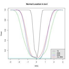
(a)

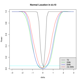
(b)

Figure 3. Empirical power for the normal location problem against $\delta N^{-\frac{1}{4}}$ alternatives, in dimension (a) $d=4$ and (b) $d=10$.

To illustrate the results above, we consider the following simulation: Consider the parametric family $\mathbb{P}_{\theta}\sim N(\theta,\mathrm{I}_{d})$, for $\theta\in\mathbb{R}^{d}$. Figure 3 shows the empirical power (out of 100 repetitions) of the tests based on the 2-NN and 6-NN graphs, the test based on the symmetrized 3-NN graph (see Appendix E for details on the limiting power of the symmetrized 3-NN test), and the Hotelling’s $T^{2}$ test, with $N_{1}=2000\text{ samples from }N(2\cdot\bm{1},\mathrm{I}_{d})\text{ and }N_{2}=1000\text{ samples from }N(2\cdot\bm{1}+\delta N^{-\frac{1}{4}}\bm{1},\mathrm{I}_{d})$, over a grid of 40 values of $\delta$ in $[-3,3]$ (smoothed out using the loess function in R), in (a) dimension 4 and (b) dimension 10. (Here, $N=N_{1}+N_{2}=3000$.) The level of the tests are set to $\alpha=0.05$. The plots show that the tests based on the NN graphs have nontrivial local power as a function of $\delta$, as predicted by the calculations above. Note that, in this case, the most powerful test is the Hotelling’s $T^{2}$-test, which has detection threshold at $N^{-\frac{1}{2}}$ and, therefore, has high power at the $N^{-\frac{1}{4}}$ scale, as seen in the plots.

Figure 4 shows the empirical power (out of 100 repetitions) of the different tests with $N_{1}=5000$ samples from $N(2\cdot\bm{1},\mathrm{I}_{d})$ and $N_{2}=3000$ samples from $N(2\cdot\bm{1}+N^{-b}\cdot\bm{h},\mathrm{I}_{d})$, where $b$ varies over a grid of 100 values in $[0,1]$, $\bm{h}=\bm{1}$ and dimension (a) $d=4$ and (b) $d=10$. Note that $b=0$ corresponds to fixed alternatives where the power is expected to be near 1 because of consistency. The level of the tests are set to $\alpha=0.25$. Note that the power of the tests based on the $K$-NN graphs transitions from $\alpha$ to 1 around $b=0.25$, which corresponds to the rate $N^{-\frac{1}{4}}$, in both dimensions, as predicted by the calculations above. On the other hand, the power of the Hotelling’s $T^{2}$ test transitions from $\alpha$ to 1 around $b=0.5$, which corresponds to the parametric rate of $N^{-\frac{1}{2}}$. The corresponding plots for the negative direction $\bm{h}=-\bm{1}$ are given in Appendix F.1.

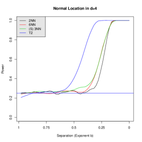
(a)

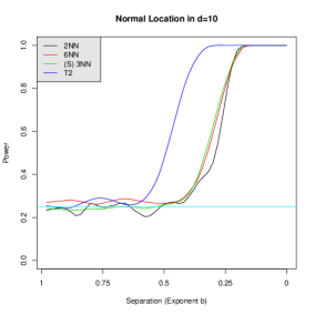
(b)

Figure 4. Empirical power in the normal location problem with $N_{1}=5000$ samples from $N(2\cdot\bm{1},\mathrm{I}_{d})$ and $N_{2}=3000$ samples from $N(2\cdot\bm{1}+N^{-b}\cdot\bm{h},\mathrm{I}_{d})$, where $b$ varies over a grid of 100 values in $[0,1]$, $\bm{h}=\bm{1}$, and dimension (a) $d=4$ and (b) $d=10$.

4.2.2. Example: Spherical normal

Let $M$ be a convex, compact subset of $\mathbb{R}^{d}$. For $\lambda>0$, define a family of densities $\phi_{M}(\cdot|\lambda^{2})$:

$$\phi_{M}\bigl{(}x|\lambda^{2}\bigr{)}=\frac{1}{Z_{M}(\lambda^{2})}e^{-\frac{1}{2\lambda^{2}}\|x\|^{2}}\quad\text{for }x\in M,$$

where $Z_{M}(\lambda^{2}):=\int_{M}e^{-\frac{1}{2\lambda^{2}}\|x\|^{2}}\,\mathrm{d}x$ is the normalizing constant. (Note that $Z_{\mathbb{R}^{d}}(\lambda^{2})=(2\pi\lambda^{2})^{\frac{d}{2}}$.) This is the $d$-dimensional spherical normal distribution $N(0,\lambda^{2}\mathrm{I}_{d})$ truncated to the set $M$. Now, consider the problem of testing (4.4) based on (4.3), given i.i.d. samples $\mathscr{X}_{N_{1}}$ and $\mathscr{Y}_{N_{2}}$ from $\phi_{M}(\cdot|\lambda_{1}^{2})$ and $\phi_{M}(\cdot|\lambda_{2}^{2})$, respectively. In this case, for $h\in\mathbb{R}$,

$$\begin{split}&\int_{M}h\cdot\nabla_{\lambda_{1}}\biggl{(}\frac{\operatorname{tr}(\mathrm{H}_{x}\phi_{M}(x|\lambda_{1}^{2}))}{\phi_{M}(x|\lambda_{1}^{2})}\biggr{)}\phi_{M}^{\frac{d-2}{d}}\bigl{(}x|\lambda_{1}^{2}\bigr{)}\\ &\quad=-\frac{Z_{M}(\frac{d\lambda_{1}^{2}}{d-2})}{Z_{M}(\lambda_{1}^{2})^{\frac{d-2}{d}}}\frac{2h}{\lambda_{1}^{5}}\bigl{(}2\mathbb{E}\|W\|^{2}-\lambda_{1}^{2}d\bigr{)},\end{split}$$ (4.14)

where $W=(W_{1},W_{2},\ldots,W_{d})^{\prime}$ are i.i.d. from the density $\phi_{M}(\cdot|\frac{d\lambda_{1}^{2}}{d-2})$ (see Section D in the supplementary material for details). Therefore (recall (4.6)),

$$a_{K,\lambda_{1}}(h)=\frac{rpC_{K,2}}{2d\sigma_{K}}\frac{Z_{M}(\frac{d\lambda_{1}^{2}}{d-2})}{Z_{M}(\lambda_{1}^{2})^{\frac{d-2}{d}}}\frac{h}{\lambda_{1}^{5}}\bigl{(}2\mathbb{E}\|W\|^{2}-\lambda_{1}^{2}d\bigr{)},$$ (4.15)

which is positive or negative depending on whether $h$ is positive or negative. Therefore, the limiting power of the test (4.3) for dimension $d\geq 9$, at the threshold $N^{\frac{1}{2}-\frac{2}{d}}\varepsilon_{N}\rightarrow h$, is $\Phi(z_{\alpha}+a_{K,\lambda_{1}}(h))$. (Note that in the simulations below we will consider the untruncated spherical normal family $\{\mathbb{P}_{\lambda}\sim N(0,\lambda^{2}\mathrm{I}_{d}):\lambda>0\}$. The limiting power in this case can be obtained by choosing $M=[-L,L]^{d}$, and taking $L\rightarrow\infty$ in (4.15).)

Now, suppose we are given i.i.d. samples $\mathscr{X}_{N_{1}}$ from $\phi_{M}(\cdot|\lambda_{1}^{2})$ and $\mathscr{Y}_{N_{2}}$ from $\phi_{M}(\cdot|\lambda_{2}^{2})$, where $\lambda_{2}=\lambda_{1}+h\delta_{N}>0$, for some $h$ fixed and $\delta_{N}\rightarrow 0$, as $N\rightarrow\infty$. Then, by Theorem 4.2, depending on the dimension and the sign of $h$ we have the following cases:

• For dimension $d\leq 8$, irrespective of the sign of $h$, the limiting power of the test (4.3) is $0$ or $1$, depending on whether $N^{\frac{1}{4}}\delta_{N}\rightarrow 0$ or $N^{\frac{1}{4}}\delta_{N}\rightarrow\infty$. At the threshold, $N^{\frac{1}{4}}\delta_{N}\rightarrow\kappa$, the limiting power is given by (4.8) or (4.9) (with $h$ replaced by $\kappa h$). This is illustrated in Figure 5, which shows the empirical power (out of 100 repetitions) of the tests based on the 2-NN and 6-NN graphs, the test based on the symmetrized 3-NN graph, and the generalized likelihood ratio test (GLR), in dimension $d=4$, with $N_{1}=12\text{,}000$ samples from $N(0,3^{2}\cdot\mathrm{I}_{d})$ and $N_{2}=6000$ samples from $N(0,(3+hN^{-b})^{2}\mathrm{I}_{d})$, where $b$ varies over a grid of 100 values in $[0,1]$ and (a) $h=2$ (b) $h=-2$. (Here, $N=N_{1}+N_{2}=18\text{,}000$.) The level of the tests are set to $\alpha=0.25$. Note that the power of the tests based on the $K$-NN graphs transitions from $\alpha$ to 1 around $b=0.25$ (irrespective of the sign of $h$), which corresponds to the rate $N^{-\frac{1}{4}}$, as shown in the calculations above. On the other hand, the power of the GLR test transitions from $\alpha$ to 1 around $b=0.5$, which corresponds to the parametric rate of $N^{-\frac{1}{2}}$.

  

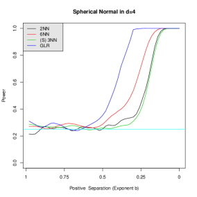
  (a)

  

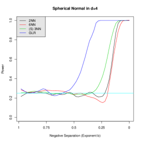
  (b)

  Figure 5. Empirical power in the spherical normal problem in dimension $d=4$ with $N_{1}=12000$ samples from $N(0,3^{2}\cdot\mathrm{I}_{d})$ and $N_{2}=6000$ samples from $N(0,(3+hN^{-b})^{2}\mathrm{I}_{d})$, where $b$ varies over a grid of 100 values in $[0,1]$ and (a) $h=2$ (b) $h=-2$.

• Next, suppose $d\geq 9$. Then depending on the sign of $h$ the following cases arise:

  • Suppose $h>0$ (then $a_{K,\lambda_{1}}(h)>0$). By (4.11), the limiting power of the test (4.3) is

    $$\begin{cases}\alpha&\text{if }N^{\frac{1}{2}-\frac{2}{d}}\delta_{N}\rightarrow 0,\\ \Phi\bigl{(}z_{\alpha}+\kappa a_{K,\lambda_{1}}(h)\bigr{)}>\alpha&\text{if }N^{\frac{1}{2}-\frac{2}{d}}\delta_{N}\rightarrow\kappa>0,\\ 1&\text{if }N^{\frac{1}{2}-\frac{2}{d}}\delta_{N}\rightarrow\infty,\end{cases}$$

    where $a_{K,\lambda_{1}}(h)$ is defined above in (4.15). Here, the detection threshold exhibits a blessing of dimensionality, improving with dimension to the parametric rate of $N^{-\frac{1}{2}}$ as the dimension $d$ grows to infinity. This is illustrated in Figure 6(a), which shows the empirical power (out of 100 repetitions) of the different tests in dimension $d=10$, with $N_{1}=300\text{,}000$ samples from $N(0,3^{2}\cdot\mathrm{I}_{d})$ and $N_{2}=200\text{,}000$ samples from $N(0,(3+hN^{-b})^{2}\mathrm{I}_{d})$, where $b$ varies over a grid of 100 values in $[0,1]$ and $h=2$. As before, the level of the tests are set to $\alpha=0.25$. Note that the power of the tests based on the $K$-NN graphs transitions from $\alpha$ to 1 around $b=\frac{1}{2}-\frac{2}{d}=0.3$, which is the predicted rate of $N^{-\frac{1}{2}+\frac{2}{d}}$. As before, the power of the GLR test transitions from 0 to 1 around $b=0.5$. To see the transitions more sharply and observe the local power of the different tests, we can zoom in at the thresholds (see Appendix F.2).

    

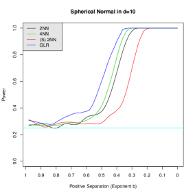
    (a)

    

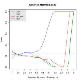
    (b)

    Figure 6. Empirical power in the spherical normal problem in dimension $d=10$ with $N_{1}$ samples from $N(0,3^{2}\cdot\mathrm{I}_{d})$ and $N_{2}$ samples from $N(0,(3+hN^{-b})^{2}\mathrm{I}_{d})$, where $b$ varies over a grid of 100 values in $[0,1]$ and (a) $h=2$ (b) $h=-2$.

  • Suppose $h<0$ (then $a_{K,\theta_{1}}(h)<0$). By Theorem 4.2, the limiting power of the test (4.3) is

    $$\begin{cases}\alpha&\text{if }N^{\frac{1}{2}-\frac{2}{d}}\delta_{N}\rightarrow 0,\\ \Phi\bigl{(}z_{\alpha}+\kappa a_{K,\theta_{1}}(h)\bigr{)}<\alpha&\text{if }N^{\frac{1}{2}-\frac{2}{d}}\delta_{N}\rightarrow\kappa>0,\\ 0&\text{if }N^{\frac{1}{2}-\frac{2}{d}}\delta_{N}\rightarrow\infty\text{ and }N^{\frac{2}{d}}\delta_{N}\rightarrow 0,\\ 1&\text{if }N^{\frac{2}{d}}\delta_{N}\rightarrow\infty.\end{cases}$$

    This is illustrated in Figure 6(b), which shows the empirical power (out of 100 repetitions) of the different tests in dimension $d=10$, with $N_{1}=200\text{,}000$ samples from $N(0,3^{2}\cdot\mathrm{I}_{d})$ and $N_{2}=100\text{,}000$ samples from $N(0,(3+hN^{-b})^{2}\mathrm{I}_{d})$, where $b$ varies over a grid of 100 values in $[0,1]$ and $h=-2$. Here, we observe the predicted non-monotonicity of the power of the $K$-NN tests. The asymptotic power starts of at the level $\alpha=0.25$, goes down to zero (predicted by the theorem at $b=\frac{1}{2}-\frac{2}{d}=0.3$), stays at zero for a while and jumps up to 1 (predicted by the theorem at $b=\frac{2}{d}=0.2$). Additional simulations zooming in to the different thresholds are given in Appendix F.2.

Appendix A Proof of CLT under general alternatives

In this section the asymptotic distribution of the two-sample test based on stabilizing geometric graphs in the Poissonized setting is derived. The section is organized as follows: Begin by recalling preliminaries about geometric graphs in Section A.1. In Section A.2 a few technical lemmas are proved, which will be required to derive the asymptotic variance of the statistic (3.3). The consistency of these tests under general alternatives (Proposition 2.1) is given in Section A.3. The proof of the conditionally centered CLT of the test statistic (Theorem 3.1) is described in Section 3.2. The CLT of the conditional mean and the proofs of Proposition 3.2 and Theorem 3.3 are given in Section A.6.

A.1. Preliminaries on stabilizing graphs and Palm theory

Given a graph functional $\mathscr{G}$, $\varphi(z,\mathscr{G}(\mathcal{Z}))$ is a measurable $\mathbb{R}^{+}$ valued function defined for all locally finite set $\mathcal{Z}\subset\mathbb{R}^{d}$ and $z\in\mathcal{Z}$. If $z\notin\mathcal{Z}$, then $\varphi(z,\mathscr{G}(\mathcal{Z})):=\varphi(z,\mathscr{G}(\mathcal{Z}\cup\{z\}))$. The function $\varphi$ is translation invariant if $\varphi(y+z,\mathscr{G}(y+\mathcal{Z}))=\varphi(z,\mathscr{G}(\mathcal{Z}))$, and scale invariant if $\varphi(az,\mathscr{G}(a\mathcal{Z}))=\varphi(z,\mathscr{G}(\mathcal{Z}))$, for all $y\in\mathbb{R}^{d}$ and $a\in\mathbb{R}^{+}$. Similar to stabilizing graph functionals, Penrose and Yukich [25] defined stabilizing functions of graph functionals as follows:

Definition A.1.

(Penrose and Yukich [25]) For any locally finite point set $\mathcal{Z}\subset\mathbb{R}^{d}$ and any integer $m\in\mathbb{N}$

$$\overline{\varphi}(\mathscr{G}(\mathcal{Z}),M):=\sup_{N\in\mathbb{N}}\left(\operatorname*{ess\,sup}_{\begin{subarray}{c}\mathcal{A}\subset\mathbb{R}^{d}\backslash B(0,M)\\ |\mathcal{A}|=N\end{subarray}}\left\{\varphi(0,\mathscr{G}(\mathcal{Z}\cap B(0,M)\cup\mathcal{A}))\right\}\right)$$

and

$$\underline{\varphi}(\mathscr{G}(\mathcal{Z}),M):=\inf_{N\in\mathbb{N}}\left(\operatorname*{ess\,inf}_{\begin{subarray}{c}\mathcal{A}\subset\mathbb{R}^{d}\backslash B(0,M)\\ |\mathcal{A}|=N\end{subarray}}\left\{\varphi(0,\mathscr{G}(\mathcal{Z}\cap B(0,M)\cup\mathcal{A}))\right\}\right),$$

where the essential supremum/infimum is taken with respect to the Lebesgue measure on $\mathbb{R}^{dN}$. The functional $\varphi$ is said to stabilize on $\mathscr{G}(\mathcal{Z})$ if

$$\liminf_{M\rightarrow\infty}\underline{\varphi}(\mathscr{G}(\mathcal{Z}),M)=\limsup_{M\rightarrow\infty}\overline{\varphi}(\mathscr{G}(\mathcal{Z}),M)=\varphi(0,\mathscr{G}(\mathcal{Z})).$$

Remark A.1.

It is important to distinguish the difference between translation/scale invariance of graph functional $\mathscr{G}$ and the translation/scale invariance a functional $\varphi(\cdot,\mathscr{G}(S))$ defined on the graph, and how it fits into the notation defined above. Throughout the paper, all graphs considered will be translation and scale invariant. However, at times we will consider functionals on these graphs which might not be scale invariant, in which case $\varphi(x,\mathscr{G}(aS))\neq\varphi(x,\mathscr{G}(S))$ (even though $\mathscr{G}(aS)=\mathscr{G}(S)$). For example, if $\varphi(0,\mathcal{P}_{\lambda})=\sum_{y\in\mathcal{P}_{\lambda}}||y||^{r}\bm{1}\{(0,y)\in E(\mathscr{G}(\mathcal{P}_{\lambda})\}=\left(\frac{1}{\lambda}\right)^{\frac{r}{d}}\sum_{y\in\mathcal{P}_{1}}||y||^{r}\bm{1}\{(0,y)\in E(\mathscr{G}(\mathcal{P}_{1})\}=\left(\frac{1}{\lambda}\right)^{\frac{r}{d}}\varphi(0,\mathcal{P}_{1})$, using $\mathcal{P}_{\lambda}=\lambda^{-1/d}\mathcal{P}_{1}$.

Hereafter, for a stabilizing function $\varphi$, define the rescaled functional

$$\varphi_{N}(x,\mathscr{G}(S))=\varphi(0,\mathscr{G}(N^{\frac{1}{d}}(S-x))).$$

It follows from [25, Lemma 3.2] that, given a density $\kappa$ in $\mathbb{R}^{d}$, under appropriate moment conditions, $\varphi_{N}(z,\mathscr{G}(\mathcal{P}_{N\kappa}))$ converges to $\varphi(0,\mathscr{G}(\mathcal{P}_{\kappa(z)}))$, if $z$ is a Lebesgue point of $\kappa$ (see definition in (A.4) below). The proof of [25, Lemma 3.2] can be easily modified to show that the same holds for any sequence of densities $\kappa_{N}\rightarrow\kappa$ uniformly, which is summarized below:

Lemma A.1.

Let $\mathscr{G}$ be a translation and scale invariant graph functional in $\mathbb{R}^{d}$, and $\phi_{N},\phi$ as in (3.1). Suppose $\varphi$ is translation invariant and almost surely stabilizing on $\mathscr{G}(\mathcal{P}_{\lambda})$, with limit $\varphi(0,\mathscr{G}(\mathcal{P}_{\lambda}))$ for all $\lambda\in(0,\infty)$, and for some $\beta>1$

$$\sup_{N\in\mathbb{N}}\sup_{\begin{subarray}{c}z\in\mathbb{R}^{d},\\ \mathcal{A}\subset\mathbb{R}^{d}\end{subarray}}\mathbb{E}\left\{\varphi_{N}(z,\mathscr{G}(\mathcal{P}_{N\phi_{N}}\cup\mathcal{A}))^{\beta}\right\}<\infty,$$ (A.1)

where the set $\mathcal{A}$ ranges over all finite subsets of $\mathbb{R}^{d}$.

1. Then, if $z$ is a Lebesgue point of $\kappa$, as $N\rightarrow\infty$,

   $$\varphi_{N}(z,\mathscr{G}(\mathcal{P}_{N\phi_{N}}))\rightarrow\varphi(0,\mathscr{G}(\mathcal{P}_{\phi(z)})),$$ (A.2)

   in expectation and in distribution.

2. For $y\in\mathbb{R}^{d}$, as $N\rightarrow\infty$,

   $$\varphi_{N}(z+N^{-\frac{1}{d}}y,\mathscr{G}(\mathcal{P}_{N\phi_{N}}))\rightarrow\varphi(0,\mathscr{G}(\mathcal{P}_{\phi(z)})),$$ (A.3)

   in expectation and in distribution. $\Box$

One aspect of the spatial independence of the Poisson process, which we will use in our proofs, is its Palm theory, which says, if conditioned to have points at particular locations, the distribution of the Poisson points elsewhere is unchanged.

Lemma A.2 (Palm theory for Poisson process [23, Theorem 1.6]).

Let $\lambda>0$ and $f$ be a density function (with respect to the Lebesgue measure) in $\mathbb{R}^{d}$ with support $\mathcal{K}$. Suppose $s\geq 1$ is a positive integer and $h(\mathcal{Y},\mathcal{X})$ is a bounded measurable function defined on all pairs of the form $(\mathcal{Y},\mathcal{X})$, where $\mathcal{X}$ is a finite subset of $\mathbb{R}^{d}$ and $\mathcal{Y}$ is a subset of $\mathcal{X}$, satisfying $h(\mathcal{Y},\mathcal{X})=0$, except when $\mathcal{Y}$ has $s$ elements. Then

$$\mathbb{E}\left(\sum_{\mathcal{Y}\subseteq\mathcal{P}_{\lambda f}}h(\mathcal{Y},\mathcal{P}_{\lambda f})\right)=\frac{\lambda^{s}}{s!}\int_{\mathcal{K}^{s}}\mathbb{E}\left(h(\{z_{1},\ldots,z_{s}\},\{z_{1}\ldots,z_{s}\}\bigcup\mathcal{P}_{\lambda f})\right)\prod_{i=1}^{s}f(z_{i})\mathrm{d}z_{i}$$

where the sum on the LHS is over all subsets $\mathcal{Y}$ of the random point set $\mathcal{P}_{\lambda f}$.

A.2. Technical lemmas

In this section a few technical lemmas required for deriving the limit of the conditional variance in Theorem 3.1 are proved. Begin with a few definitions: For $A\subset\mathbb{R}^{d}$, denote by $|A|$ the Lebesgue measure of the set $A$. A point $x\in\mathbb{R}^{d}$ is a Lebesgue point of $\phi$ if

$$\lim_{\varepsilon\rightarrow 0}\frac{1}{|B(x,\varepsilon)|}\int_{B(x,\varepsilon)}|\phi(y)-\phi(x)|\mathrm{d}y=0,$$ (A.4)

where $B(x,\varepsilon)$ is the Euclidean ball in $\mathbb{R}^{d}$ with center at $x$ and radius $\varepsilon$. Almost every point $x\in\mathbb{R}^{d}$ is a Lebesgue point of $\phi$ [28, Theorem 7.7].

Let $\phi_{N},\phi$ as in (3.1), and $h:\mathbb{R}^{d}\times\mathbb{R}^{d}\rightarrow[0,1]$ a symmetric and jointly measurable function, such that for almost every $x\in\mathbb{R}^{d}$, $h(x,\cdot)$ is measurable and $x$ a Lebesgue point of the function $\phi(\cdot)h(x,\cdot)$. Define

$$\kappa_{N}(z)=\sum_{w\in\mathcal{P}_{N\phi_{N}}}h(z,w)\bm{1}\{(z,w)\in E(\mathscr{G}(\mathcal{P}_{N\phi_{N}}))\}.$$ (A.5)

Lemma A.3.

Let $\mathscr{G}$ be a translation and scale invariant graph functional in $\mathbb{R}^{d}$ which satisfies the $\beta$-degree moment condition (2.1) for some $\beta>2$. Then for $h:\mathbb{R}^{d}\times\mathbb{R}^{d}\rightarrow[0,1]$ as above

$$\lim_{N\rightarrow\infty}\mathbb{E}\kappa_{N}(z)=h(z,z)\mathbb{E}\Delta_{0}^{\uparrow},$$ (A.6)

if $z$ is a Lebesgue point of $\phi$ and $h(z,\cdot)\phi$, and where $\Delta_{0}^{\uparrow}$ is defined in (3.6). Moreover, as $N\rightarrow\infty$,

$$\frac{1}{N}\sum_{z\in\mathcal{P}_{N\phi_{N}}}\kappa_{N}(z)\stackrel{{\scriptstyle L^{2}}}{{\rightarrow}}\mathbb{E}\Delta_{0}^{\uparrow}\int_{\mathbb{R}^{d}}h(z,z)\phi(z)\mathrm{d}z.$$ (A.7)

The lemma is proved below in Section A.2.1. The same proof shows that

$$\frac{1}{N}\sum_{z\in\mathcal{P}_{N\phi_{N}}}\kappa_{N}^{+}(z)\stackrel{{\scriptstyle L^{2}}}{{\rightarrow}}\mathbb{E}\Delta_{0}^{+}\int_{\mathbb{R}^{d}}h(z,z)\phi(z)\mathrm{d}z,$$ (A.8)

where $\kappa^{+}_{N}(z)=\sum_{w\in\mathcal{P}_{N\phi_{N}}}h(z,w)\bm{1}\{(z,w),(z,w)\in E(\mathscr{G}(\mathcal{P}_{N\phi_{N}}))\}$ and $\Delta_{0}^{+}$ is as defined in (3.6).

Next, define $\omega^{\uparrow},\omega^{\downarrow}:\mathbb{R}^{d}\times\mathbb{R}^{d}\times\mathbb{R}^{d}\rightarrow[0,1]$ as follows:

$$\omega^{\uparrow}(x,y,z)=\frac{pq^{2}f(x)g(y)g(z)}{(pf(x)+qg(x))(pf(y)+qg(y))(pf(z)+qg(z))},$$ (A.9)

and

$$\omega^{\downarrow}(x,y,z)=\frac{p^{2}qg(x)f(y)f(z)}{(pf(x)+qg(x))(pf(y)+qg(y))(pf(z)+qg(z))}.$$ (A.10)

Let

$$\tau_{N}^{\uparrow}(z):=\frac{1}{2}\sum_{w_{1}\neq w_{2}\in\mathcal{P}_{N\phi_{N}}}\omega^{\uparrow}(z,w_{1},w_{2})\bm{1}\{(z,w_{1}),(z,w_{2})\in E(\mathscr{G}(\mathcal{P}_{N\phi_{N}}))\},$$

and

$$\tau_{N}^{\downarrow}(z):=\frac{1}{2}\sum_{w_{1}\neq w_{2}\in\mathcal{P}_{N\phi_{N}}}\omega^{\downarrow}(z,w_{1},w_{2})\bm{1}\{(w_{1},z),(w_{2},z)\in E(\mathscr{G}(\mathcal{P}_{N\phi_{N}}))\}.$$

where $\phi_{N}$ is defined in (3.1).

Lemma A.4.

Let $\mathscr{G}$ be an translation and scale invariant graph functional in $\mathbb{R}^{d}$ which satisfies the $\beta$-degree moment condition (2.1) for some $\beta>4$. Then

$$\frac{1}{N}\sum_{z\in\mathcal{P}_{N\phi_{N}}}\tau_{N}^{\uparrow}(h,z) \stackrel{{\scriptstyle L^{2}}}{{\rightarrow}} \mathbb{E}T_{2}^{\uparrow}\int_{\mathbb{R}^{d}}\omega^{\uparrow}(z,z,z)\phi(z)\mathrm{d}z,$$ (A.11)

for $\omega^{\uparrow}$ as in (A.9). The same result holds for $\tau_{N}^{\downarrow}(h,z)$, with $\mathbb{E}T_{2}^{\uparrow}$ replaced by $\mathbb{E}T_{2}^{\downarrow}$, and $\omega^{\uparrow}$ replaced by $\omega^{\downarrow}$.

The proof of Lemma A.3 is given in Section A.2.1. The proof of Lemma A.4 is described in Section A.2.2.

A.2.1. Proof of Lemma A.3

The proof of Lemma A.3 is organized as follows: Begin with the proof of (A.6) below. This together with uniform integrability, which follows from the degree moment condition (2.1), implies the convergence in expectation in (A.7). Following this the convergence of (A.7) in $L^{2}$ is shown, by computing the limit of the second moment.

Proof of (A.6) and Convergence in Expectation: Fix $K>0$. By the Palm theory of Poisson processes [23, Theorem 1.6],

$$\mathbb{E}\sum_{w\in\mathcal{P}_{N\phi_{N}}}|h(z,w)-h(z,z)|\bm{1}\{w\in B(z,KN^{-\frac{1}{d}})\}$$ (A.12)

$$= N\int_{B(z,KN^{-\frac{1}{d}})}|h(z,w)-h(z,z)|\phi_{N}(w)\mathrm{d}w,$$

which tends to zero as $N\rightarrow\infty$, if $z$ is a Lebesgue point of both $\phi$ and $h(z,\cdot)\phi(\cdot)$ (using $\phi_{N}\rightarrow\phi$ uniformly and $|h|\leq 1$). Since $h$ has range $[0,1]$, this implies that

$$\limsup_{N\rightarrow\infty}\mathbb{E}\sum_{w\in\mathcal{P}_{N\phi_{N}}}|h(z,w)-h(z,z)|\bm{1}\{(z,w)\in\mathscr{G}(\mathcal{P}_{N\phi_{N}})\}$$

$$\leq \limsup_{N\rightarrow\infty}\mathbb{E}d_{K}^{\uparrow}(z,\mathscr{G}(\mathcal{P}_{N\phi_{N}})),$$ (A.13)

where $d_{K}^{\uparrow}(z,\mathscr{G}(\mathcal{P}_{N\phi_{N}})$ is the number of edges $(z,w)\in E(\mathscr{G}(\mathcal{P}_{N\phi_{N}}))$ incident on $z$ such that $w\notin B(z,KN^{-\frac{1}{d}})$.

Since $\mathscr{G}$ is stabilizes on $\mathcal{P}_{\lambda}$ for all $\lambda\in(0,\infty)$ (as in Definition 1.3), the functions $d^{\uparrow}$ and $d_{K}^{\uparrow}$ defined on $\mathscr{G}$ stabilizes on $\mathcal{P}_{\lambda}$, for all $\lambda\in(0,\infty)$ (as in Definition A.1). Therefore, by Lemma A.1,

$$\limsup_{K\rightarrow\infty}\limsup_{N\rightarrow\infty}\mathbb{E}d_{K}^{\uparrow}(z,\mathscr{G}(\mathcal{P}_{N\phi_{N}})=\limsup_{K\rightarrow\infty}\mathbb{E}d_{K}^{\uparrow}(0,\mathscr{G}(\mathcal{P}_{\phi(z)})=0.$$ (A.14)

Now, recall the definition of $\kappa_{N}(\cdot)$ from (A.5). Then from (A.2.1) and (A.14), it follows that for every $z$ which is a Lebesgue point of $\phi$ and $h(z,\cdot)\phi$,

$$\lim_{N\rightarrow\infty}\mathbb{E}\kappa_{N}(z)= h(z,z)\lim_{N\rightarrow\infty}\mathbb{E}d^{\uparrow}(z,\mathscr{G}(\mathcal{P}_{N\phi_{N}}))$$

$$= h(z,z)\mathbb{E}d^{\uparrow}(0,\mathscr{G}(\mathcal{P}_{\phi(z)}))$$

$$= h(z,z)\mathbb{E}d^{\uparrow}(0,\mathscr{G}(\mathcal{P}_{1})),$$ (A.15)

where the last equality uses $\mathscr{G}$ is scale invariant. Therefore, as $N\rightarrow\infty$

$$\mathbb{E}\left(\frac{1}{N}\sum_{z\in\mathcal{P}_{N\phi_{N}}}\kappa_{N}(z)\right)=\int\phi_{N}(z)\mathbb{E}\kappa_{N}(z)\rightarrow \mathbb{E}\Delta_{0}^{\uparrow}\int\phi(z)h(z,z)\mathrm{d}z$$

$$:= \mu(\mathscr{G},h),$$ (A.16)

by (A.15) and the Dominated Convergence Theorem.

Proof of (A.7) (Convergence in $L^{2}$): By the Palm theory of Poisson processes,

$$\mathbb{E} \left(\frac{1}{N}\sum_{z\in\mathcal{P}_{N\phi_{N}}}\kappa_{N}(z)\right)^{2}$$

$$=\frac{1}{N}\int\phi_{N}(z)\mathbb{E}\kappa_{N}^{2}(z)\mathrm{d}z+\int\phi_{N}(z_{1})\phi_{N}(z_{2})\mathbb{E}\kappa_{N}(z_{1})\kappa_{N}(z_{2})\mathrm{d}z_{1}\mathrm{d}z_{2}.$$ (A.17)

Now, since $h$ is bounded in $[0,1]$, $\mathbb{E}\kappa_{N}(z)^{2}\leq\mathbb{E}\left(d^{\uparrow}(z,\mathcal{P}_{N\phi_{N}})\right)^{2}\rightarrow\mathbb{E}\left(d^{\uparrow}(z,\mathcal{P}_{\phi(z)})\right)^{2}$, as (2.1) holds for $\beta>2$. Thus, $\int\phi_{N}(z)\mathbb{E}\kappa_{N}^{2}(z)\mathrm{d}z=O(1)$, and the first term in (A.2.1) goes to 0 as $N\rightarrow\infty$. Therefore, it suffices to consider the second term. Fix $K>0$ and let $z_{1}$ and $z_{2}$ be Lebesgue points of $\phi$. Define $A(z_{1},z_{2}):=B(z_{1},KN^{-\frac{1}{d}})\times B(z_{2},KN^{-\frac{1}{d}})\subset\mathbb{R}^{d}\times\mathbb{R}^{d}$. Then by triangle inequality, for almost all $z_{1},z_{2}$

$$N^{2}\int_{A(z_{1},z_{2})}|\phi(w_{1})\phi(w_{2})-\phi(z_{1})\phi(z_{2})|\mathrm{d}w_{1}\mathrm{d}w_{2}\rightarrow 0,$$ (A.18)

as $N\rightarrow\infty$.

Similarly, if $z_{1},z_{2}$ are Lebesgue points of $h(z_{1},\cdot)\phi(\cdot)$ and $h(z_{2},\cdot)\phi(\cdot)$, respectively, then as $N\rightarrow\infty$

$$N^{2}\int_{A(z_{1},z_{2})}|h(z_{1},w_{1})h(z_{2},w_{2})\phi(w_{1})\phi(w_{2})-h(z_{1},z_{1})h(z_{2},z_{2})\phi(z_{1})\phi(z_{2})|\mathrm{d}w_{1}\mathrm{d}w_{2}$$ (A.19)

$$\leq N^{2}\int_{A(z_{1},z_{2})}\phi(w_{2})h(z_{2},w_{2})|h(z_{1},w_{1})\phi(w_{1})-h(z_{1},z_{1})\phi(z_{1})|\mathrm{d}w_{1}\mathrm{d}w_{2}$$

$$+ N^{2}\int_{A(z_{1},z_{2})}h(z_{1},z_{1})\phi(z_{1})|h(z_{2},w_{2})\phi(w_{2})-h(z_{2},z_{2})\phi(z_{2})|\mathrm{d}w_{1}\mathrm{d}w_{2}$$

$$\rightarrow 0.$$

Now, let $S_{w_{1},w_{2}}=\{w_{1},w_{2}\in\mathcal{P}_{N\phi_{N}}:(z_{1},w_{1}),(z_{2},w_{2})\in E(\mathscr{G}(\mathcal{P}_{N\phi_{N}}))\}$. Then, since $h$ has range $[0,1]$, (A.18) and (A.19) gives

$$\limsup_{N\rightarrow\infty}\mathbb{E}\sum_{S_{w_{1},w_{2}}}|h(z_{1},w_{1})h(z_{2},w_{2})-h(z_{1},z_{1})h(z_{2},z_{2})|$$ (A.20)

$$\lesssim \limsup_{N\rightarrow\infty}T_{N,K}(z_{1})+\limsup_{N\rightarrow\infty}T_{N,K}(z_{2}).$$

where

$$\limsup_{N\rightarrow\infty}T_{N,K}(z_{1})= \lim_{N\rightarrow\infty}\mathbb{E}d_{K}^{\uparrow}(z_{1},\mathscr{G}(\mathcal{P}_{N\phi_{N}})d^{\uparrow}(z_{2},\mathscr{G}(\mathcal{P}_{N\phi_{N}})$$

$$\leq \left(\mathbb{E}\{d_{K}^{\uparrow}(0,\mathscr{G}(\mathcal{P}_{\phi(z_{1})})\}^{2}\mathbb{E}\{d^{\uparrow}(0,\mathscr{G}(\mathcal{P}_{\phi(z_{2})}\}^{2}\right)^{\frac{1}{2}},$$ (A.21)

by Lemma A.1, since (2.1) holds for $\beta>2$.

Similarly,

$$\limsup_{N\rightarrow\infty}T_{N,K}(z_{2})= \lim_{N\rightarrow\infty}\mathbb{E}d^{\uparrow}(z_{1},\mathscr{G}(\mathcal{P}_{N\phi_{N}})d_{K}^{\uparrow}(z_{2},\mathscr{G}(\mathcal{P}_{N\phi_{N}})$$

$$\leq \left(\mathbb{E}\{d^{\uparrow}(0,\mathscr{G}(\mathcal{P}_{\phi(z_{1})})\}^{2}\mathbb{E}\{d_{K}^{\uparrow}(0,\mathscr{G}(\mathcal{P}_{\phi(z_{2})}\}^{2}\right)^{\frac{1}{2}}.$$ (A.22)

Combining (A.2.1) and (A.2.1) and taking $K\rightarrow\infty$ it follows that the LHS of (A.20) goes to zero. Therefore,

$$\lim_{N\rightarrow\infty}\mathbb{E}\kappa_{N}(z_{1})\kappa_{N}(z_{2})$$

$$= \lim_{N\rightarrow\infty}\sum_{w_{1},w_{2}\in\mathcal{P}_{N\phi_{N}}}h(z_{1},w_{1})h(z_{2},w_{2})\bm{1}\{(z_{1},w_{1}),(z_{2},w_{2})\in E(\mathscr{G}(\mathcal{P}_{N\phi_{N}}))$$

$$= h(z_{1},z_{1})h(z_{2},z_{2})\lim_{N\rightarrow\infty}\mathbb{E}d^{\uparrow}(z_{1},\mathscr{G}(\mathcal{P}_{N\phi_{N}})d^{\uparrow}(z_{2},\mathscr{G}(\mathcal{P}_{N\phi_{N}})$$ (A.23)

for $z_{1},z_{2}$ Lebesgue points of $\phi$ and $h(z_{1},\cdot)\phi$ and $h(z_{2},\cdot)\phi$, respectively. Now, by a modification of the coupling argument used in Lemma A.1, similar to the proof of [25, Lemma 3.1], it can be shown that

$$\lim_{N\rightarrow\infty}\mathbb{E}d^{\uparrow}(z_{1},\mathscr{G}(\mathcal{P}_{N\phi_{N}})d^{\uparrow}(z_{2},\mathscr{G}(\mathcal{P}_{N\phi_{N}})= \mathbb{E}d^{\uparrow}(0,\mathscr{G}(\mathcal{P}_{\phi(z_{1})})\mathbb{E}d^{\uparrow}(0,\mathscr{G}(\mathcal{P}_{\phi(z_{2})})$$

$$= \{\mathbb{E}d^{\uparrow}(0,\mathscr{G}(\mathcal{P}_{1})\}^{2},$$ (A.24)

where the last step uses $\mathscr{G}$ is scale invariant. Combining (A.2.1) with (A.2.1) gives

$$\lim_{N\rightarrow\infty}\mathbb{E}\kappa_{N}(z_{1})\kappa_{N}(z_{2})=\{\mathbb{E}d^{\uparrow}(0,\mathscr{G}(\mathcal{P}_{1})\}^{2}h(z_{1},z_{1})h(z_{2},z_{2}).$$

Thus, taking limit as $N\rightarrow\infty$ in (A.2.1) gives

$$\lim_{N\rightarrow}\mathbb{E}\left(\frac{1}{N}\sum_{z\in\mathcal{P}_{N\phi_{N}}}\kappa_{N}(z)\right)^{2} = \mu(\mathscr{G},h)^{2},$$ (A.25)

where $\mu(\mathscr{G},h)$ is defined in (A.2.1). Combining (A.2.1) and (A.25) gives the $L^{2}$ convergence in (A.7).

Proof of (A.8): It follows from (A.12), (A.2.1), and (A.14) that if $z$ is a Lebesgue point of both $\phi$ and $h(z,\cdot)\phi(\cdot)$, then

$$\mathbb{E}\sum_{w\in\mathcal{P}_{N\phi_{N}}}|h(z,w)-h(z,z)|\bm{1}\{(z,w),(w,z)\in\mathscr{G}(\mathcal{P}_{N\phi_{N}})\}\rightarrow 0.$$

Lemma A.1 then implies that $\mathbb{E}\kappa_{N}^{+}(z)\rightarrow\mathbb{E}\Delta^{+}_{0}h(z,z)$, where $\Delta^{+}_{0}$ is as defined in (3.6). This shows convergence in expectation. The $L^{2}$ convergence is similar to the proof of (A.7).

A.2.2. Proof of Lemma A.4

The proof is very similar to Lemma A.3. Without loss of generality consider the function $\omega^{\uparrow}$ defined in (A.9) (the proof for $\omega^{\downarrow}$ is identical).

Fix $K>0$. Define $B^{2}(z):=B(z,KN^{-\frac{1}{d}})\times B(z,KN^{-\frac{1}{d}})$, then by Palm theory,

$$\mathbb{E}\sum_{w_{1}\neq w_{2}\in\mathcal{P}_{N\phi_{N}}}\left|\omega^{\uparrow}(z,w_{1},w_{2})-\omega^{\uparrow}(z,z,z)\right|\bm{1}\{w_{1},w_{2}\in B(z,KN^{-\frac{1}{d}})\}$$ (A.26)

$$= N^{2}\int_{B^{2}(z)}\left|\omega^{\uparrow}(z,w_{1},w_{2})-\omega^{\uparrow}(z,z,z)\right|\phi(w_{1})\phi(w_{2})\mathrm{d}w_{1}\mathrm{d}w_{2}+o(1),$$

since $\phi_{N}\rightarrow\phi$ uniformly.

Note that

$$\omega^{\uparrow}(z,w_{1},w_{2})\phi(w_{1})\phi(w_{2})=\frac{pq^{2}f(z)g(w_{1})g(w_{2})}{pf(z)+qg(z)}.$$

Therefore, if $z$ is a Lebesgue point of both $f$ and $g$, then $(z,z)$ is the Lebesgue point of $\omega^{\uparrow}(z,\cdot,\cdot)\phi(\cdot)\phi(\cdot)$, and as $N\rightarrow\infty$,

$$N^{2}\int_{B^{2}(z)}|\omega^{\uparrow}(z,w_{1},w_{2})\phi(w_{1})\phi(w_{2})-\omega^{\uparrow}(z,z,z)\phi^{2}(z)|\mathrm{d}w_{1}\mathrm{d}w_{2}\rightarrow 0.$$ (A.27)

Moreover,

$$\phi(z)\lim_{N\rightarrow\infty}N^{2}\int_{B^{2}(z)}|\phi(w_{2})-\phi(z)|\mathrm{d}w_{1}\mathrm{d}w_{2}=0.$$ (A.28)

and by the Lebesgue differentiation theorem

$$\lim_{N\rightarrow\infty}N^{2}\int_{B(z,KN^{-\frac{1}{d}})}|\phi(w_{1})-\phi(z)|\mathrm{d}y_{1}\int_{B(z,KN^{-\frac{1}{d}})}\phi(w_{2})\mathrm{d}w_{2}=0.$$ (A.29)

Combining (A.28) and (A.29) gives

$$\lim_{N\rightarrow\infty}N^{2}\int_{B^{2}(z)}\omega^{\uparrow}(z,z,z)|\phi_{N}(w_{1})\phi(w_{2})-\phi^{2}(z)|\mathrm{d}w_{1}\mathrm{d}w_{2}\rightarrow 0.$$ (A.30)

The triangle inequality combined with (A.27) and (A.30) implies that the RHS of (A.26) goes to 0 as $N\rightarrow\infty$. This implies that

$$\mathbb{E}\sum_{w_{1}\neq w_{2}\in\mathcal{P}_{N\phi_{N}}} \left|\omega^{\uparrow}(z,w_{1},w_{2})-\omega^{\uparrow}(z,z,z)\right|\bm{1}\{(z,w_{1}),(z,w_{1})\in E(\mathscr{G}(\mathcal{P}_{N\phi_{N}}))\}$$

$$\leq 2\mathbb{E}T_{2,K}^{\uparrow}(z,\mathscr{G}(\mathcal{P}_{N\phi_{N}}))+o(1),$$ (A.31)

where

$$T_{2,K}^{\uparrow}( z,\mathscr{G}(\mathcal{P}_{N\phi_{N}}))$$

$$= \sum_{w\in\mathcal{P}_{N\phi_{N}}}\bm{1}\{(z,w_{1}),(z,w_{2})\in E(\mathscr{G}(\mathcal{P}_{N\phi_{N}}))\}\bm{1}\{w_{1}\text{ or }w_{2}\notin B(z,KN^{-\frac{1}{d}})\}.$$

Now, since $\mathscr{G}$ stabilizes on $\mathcal{P}_{\lambda}$ for all $\lambda\in(0,\infty)$, the function $T_{2}^{\uparrow}$ and hence $T_{2,K}^{\uparrow}$ stabilizes on $\mathcal{P}_{\lambda}$, for all $\lambda\in(0,\infty)$. Moreover, $T_{2,K}^{\uparrow}(z,\mathscr{G}(\mathcal{P}_{N\phi_{N}}))$ satisfies the bounded moment condition (A.1) for $\beta>1$, since $d^{\uparrow}(z,\mathscr{G}(\mathcal{P}_{N\phi_{N}})$ satisfies (2.1) for some $\beta>2$. Therefore, by Lemma A.1,

$$\limsup_{K\rightarrow\infty}\limsup_{N\rightarrow\infty}\mathbb{E}T_{2,K}^{\uparrow}(z,\mathscr{G}(\mathcal{P}_{N\phi_{N}})=0.$$ (A.32)

From (A.2.2) and (A.32) it follows that for every $z$ which is a Lebesgue point of both $f$ and $g$,

$$\lim_{N\rightarrow\infty}\mathbb{E}\tau_{N}^{\uparrow}(z) = \omega^{\uparrow}(z,z,z)\lim_{N\rightarrow\infty}\mathbb{E}2T_{2}^{\uparrow}(z,\mathscr{G}(\mathcal{P}_{N\phi_{N}}))$$ (A.33)

$$= 2\omega^{\uparrow}(z,z,z)\mathbb{E}T_{2}^{\uparrow}(0,\mathscr{G}(\mathcal{P}_{\phi(z)}))$$

$$= 2\omega^{\uparrow}(z,z,z)\mathbb{E}T_{2}^{\uparrow},$$ (A.34)

where (A.33) uses Lemma A.1 and (A.34) uses $\mathscr{G}$ is scale invariant. Therefore, by the Dominated Convergence Theorem,

$$\lim_{N\rightarrow\infty}\mathbb{E}\left(\frac{1}{N}\sum_{z\in\mathcal{P}_{N\phi_{N}}}\tau_{N}^{\uparrow}(z)\right) = \lim_{N\rightarrow\infty}\int\phi_{N}(z)\mathbb{E}\tau_{N}^{\uparrow}(z)$$ (A.35)

$$\rightarrow \mathbb{E}T_{2}^{\uparrow}\int\phi(z)\omega^{\uparrow}(z,z,z)\mathrm{d}z.$$

Now, as in Lemma A.3, it can be shown that the second moment of the quantity $\frac{1}{N}\sum_{z\in\mathcal{P}_{N\phi_{N}}}\tau_{N}^{\uparrow}(z)$ converges to $\left(\mathbb{E}T_{2}^{\uparrow}\int\phi(z)\omega^{\uparrow}(z,z,z)\mathrm{d}z\right)^{2}$. This proves the $L^{2}$ convergence of (A.11).

A.3. Proof of Proposition 2.1

Recall from (1.8) the definition of $T(\mathscr{G}(\mathcal{Z}_{N}^{\prime}))$. Define

$$h_{N}(x,y)=\frac{N_{1}N_{2}f(x)g(y)}{(N_{1}f(x)+N_{2}g(x))(N_{1}f(y)+N_{2}g(y))}.$$

Note that $h_{N}(x,y)\rightarrow h(x,y)=\frac{pqf(x)g(y)}{(pf(x)+qg(x))(pf(y)+qg(y))}$, uniformly in $x,y\in\mathbb{R}^{d}$ as $N\rightarrow\infty$. Then, with $\phi_{N}$ and $\phi$ as in (3.1),

$$\frac{1}{N}\mathbb{E}(T(\mathscr{G}(\mathcal{Z}_{N}^{\prime}))|\mathcal{F}) =\frac{1}{N}\sum_{1\leq i\neq j\leq L_{N}}h_{N}(Z_{i},Z_{j})\bm{1}\{(Z_{i},Z_{j})\in E(\mathscr{G}(\mathcal{Z}_{N}^{\prime}))\}$$

$$=\frac{1}{N}\sum_{1\leq i\neq j\leq L_{N}}h(Z_{i},Z_{j})\bm{1}\{(Z_{i},Z_{j})\in E(\mathscr{G}(\mathcal{Z}_{N}^{\prime}))\}+o(1)$$

$$\stackrel{{\scriptstyle D}}{{=}}\frac{1}{N}\sum_{z,w\in\mathcal{P}_{N\phi_{N}}}h(z,w)\bm{1}\{(z,w)\in E(\mathscr{G}(\mathcal{Z}_{N}^{\prime}))\}+o(1)$$

$$\stackrel{{\scriptstyle L^{2}}}{{\rightarrow}}\mathbb{E}\Delta_{0}^{\uparrow}\int h(z,z)\phi(z)\mathrm{d}z=\frac{\mathbb{E}\Delta_{0}^{\uparrow}}{2}(1-\delta(f,g,p)),$$ (A.36)

where the last step uses Lemma A.7 (recall that $\Delta_{0}^{\uparrow}=d(0,\mathscr{G}(\mathcal{P}_{1}))$, and $\delta(f,g,p))$ is defined in (2.2)).

The limit in (A.36) shows convergence in expectation. To show convergence in probability, compute

$$\operatorname{Var}(T(\mathscr{G}(\mathcal{Z}_{N}^{\prime})))=\mathbb{E}(\operatorname{Var}(T(\mathscr{G}(\mathcal{Z}_{N}^{\prime}))|\mathcal{F}))+\operatorname{Var}(\mathbb{E}(T(\mathscr{G}(\mathcal{Z}_{N}^{\prime}))|\mathcal{F})).$$

From (A.36) it follows that $\operatorname{Var}(\frac{1}{N}\mathbb{E}(T(\mathscr{G}(\mathcal{Z}_{N}^{\prime}))|\mathcal{F}))\rightarrow 0$. Moreover, by Lemma A.5 below,

$$\frac{1}{N}\mathbb{E}(\operatorname{Var}(T(\mathscr{G}(\mathcal{Z}_{N}^{\prime}))|\mathcal{F}))=\mathbb{E}(\operatorname{Var}(\mathcal{R}_{1}(\mathscr{G}(\mathcal{Z}_{N}^{\prime}))|\mathcal{F}))=\kappa_{\mathscr{G}}^{2}.$$

This implies $\frac{1}{N^{2}}\operatorname{Var}(T(\mathscr{G}(\mathcal{Z}_{N}^{\prime})))\rightarrow 0$, completing the proof of (2.3).

A.4. Proof of Theorem 3.1

This section is organized as follows: Section A.4.1 below derives the limit of the conditional variance (3.9), using results proved in Section A.2. The proof of the CLT is given in Section A.4.2.

A.4.1. Limiting conditional variance

The limit of the conditional variance $\operatorname{Var}(\mathcal{R}_{1}(\mathscr{G}(\mathcal{Z}_{N}^{\prime}))|\mathcal{F})$ can be computed in terms of the graph functional $\mathscr{G}$ and the unknown densities $f$ and $g$.

Lemma A.5.

Let $\mathscr{G}$ as in Theorem 3.1 and $\mathcal{R}_{1}(\mathscr{G}(\mathcal{Z}_{N}^{\prime}))$ as in (3.3). Then,

$$\operatorname{Var}(\mathcal{R}_{1}(\mathscr{G}(\mathcal{Z}_{N}^{\prime}))|\mathcal{F})\stackrel{{\scriptstyle L^{2}}}{{\rightarrow}}\kappa_{\mathscr{G}}^{2},$$ (A.37)

where $\kappa_{\mathscr{G}}$ is defined in (3.9).

Proof.

Define the function $h_{N}:\mathbb{R}^{d}\times\mathbb{R}^{d}\rightarrow[0,1]$ as

$$h_{N}(x,y)=\frac{N_{1}N_{2}f(x)g(y)}{(N_{1}f(x)+N_{2}g(x))(N_{1}f(y)+N_{2}g(y))}.$$ (A.38)

By construction $\mathcal{Z}_{N}^{\prime}$ is a Poisson process in $\mathbb{R}^{d}$ with intensity function $N\phi_{N}$, where $\phi_{N}\rightarrow\phi$ uniformly as $N\rightarrow\infty$ (as defined in (3.1)). Recall that $\psi(c_{x},c_{y})=\bm{1}\{c_{x}=1,c_{y}=2\}$, which implies $\mathbb{P}(\psi(c_{x},c_{y})|\mathcal{F})=h_{N}(x,y)$. Moreover,

$$h_{N}(x,y)\rightarrow h(x,y)=\frac{pqf(x)g(y)}{(pf(x)+qg(x))(pf(y)+qg(y))},$$

uniformly in $x,y\in\mathbb{R}^{d}$ as $N\rightarrow\infty$.

Now, let

$$V_{x,y}:=(\psi(c_{x},c_{y})-h_{N}(x,y))\bm{1}\{(x,y)\in E(\mathscr{G}(\mathcal{Z}_{N}^{\prime}))\}.$$ (A.39)

Then by (3.3), $\mathcal{R}_{1}(\mathscr{G}(\mathcal{Z}_{N}^{\prime})):=\frac{1}{\sqrt{N}}\sum_{x,y\in\mathcal{Z}_{N}^{\prime}}V_{x,y}$. Therefore,

$$\operatorname{Var} (\mathcal{R}_{1}(\mathscr{G}(\mathcal{Z}_{N}^{\prime}))|\mathcal{F})$$

$$= \frac{1}{N}\sum_{x\neq y\in\mathcal{Z}_{N}^{\prime}}\operatorname{Var}(V_{x,y}|\mathcal{F})+\frac{2}{N}\left\{\sum_{x\in\mathcal{Z}_{N}^{\prime}}\sum_{\begin{subarray}{c}y,z\in\mathcal{Z}_{N}^{\prime}\\ y<z\end{subarray}}\operatorname{Cov}(V_{x,y},V_{x,z}|\mathcal{F})+\sum_{x\in\mathcal{Z}_{N}^{\prime}}\sum_{\begin{subarray}{c}y,z\in\mathcal{Z}_{N}^{\prime}\\ y<z\end{subarray}}\operatorname{Cov}(V_{y,x},V_{z,x}|\mathcal{F})\right\}$$

$$\;\;\;\;\;\;\;\;\;\;\;\;\;\;\;\;\;\;\;\;\;\;\;\;\;\;+\frac{2}{N}\left\{\sum_{x\in\mathcal{Z}_{N}^{\prime}}\sum_{\begin{subarray}{c}y,z\in\mathcal{Z}_{N}^{\prime}\\ y<z\end{subarray}}\operatorname{Cov}(V_{x,y},V_{z,x}|\mathcal{F})+\sum_{x<y\in\mathcal{Z}_{N}^{\prime}}\operatorname{Cov}(V_{x,y},V_{y,x}|\mathcal{F})\right\}.$$ (A.40)

By Lemma A.3, as $N\rightarrow\infty$,

$$\frac{1}{N}\sum_{x,y\in\mathcal{Z}_{N}^{\prime}} \operatorname{Var}(V_{x,y}|\mathcal{F})$$

$$= \frac{1}{N}\sum_{x,y\in\mathcal{Z}_{N}^{\prime}}\Big{\{}h_{N}(x,y)(1-h_{N}(x,y))\Big{\}}\bm{1}\{(x,y)\in E(\mathscr{G}(\mathcal{Z}_{N}^{\prime}))\}$$

$$\stackrel{{\scriptstyle L_{2}}}{{\rightarrow}} \mathbb{E}\Delta^{\uparrow}_{0}\int\Big{\{}h(x,x)(1-h(x,x))\Big{\}}\phi(x)\mathrm{d}x.$$

It remains to compute the limit of the covariance term in (A.4.1). To this end, observe that

$$\operatorname{Cov}(V_{x,y}, V_{x,z}|\mathcal{F})$$

$$= \{\omega_{N}(x,y,z)-h_{N}(x,y)h_{N}(x,z)\}\bm{1}\{(x,y),(x,z)\in E(\mathscr{G}(\mathcal{Z}_{N}^{\prime}))\},$$

where

$$\omega_{N}^{\uparrow}(x,y,z) := \frac{N_{1}N_{2}^{2}f(x)g(y)g(z)}{(N_{1}f(x)+N_{2}g(x))(N_{1}f(y)+N_{2}g(y))(N_{1}f(z)+N_{2}g(z))}$$

$$\rightarrow \omega^{\uparrow}(x,y,z),$$

where $\omega^{\uparrow}(\cdot,\cdot,\cdot)$ is defined in (A.9). The convergence above is uniformly in $x,y,z\in\mathbb{R}^{d}$, as $N\rightarrow\infty$. Therefore, by Lemma A.4,

$$\frac{1}{N}\sum_{x\in\mathcal{Z}_{N}^{\prime}}\sum_{\begin{subarray}{c}y,z\in\mathcal{Z}_{N}^{\prime}\\ y<z\end{subarray}} \operatorname{Cov}(V_{x,y},V_{x,z}|\mathcal{F})$$

$$\stackrel{{\scriptstyle L_{2}}}{{\rightarrow}} \mathbb{E}T_{2}^{\uparrow}\int\left\{\omega^{\uparrow}(x,x,x)-h^{2}(x,x)\right\}\phi(x)\mathrm{d}x,$$ (A.41)

where $T_{2}^{\uparrow}=T_{2}^{\uparrow}(0,\mathscr{G}(\mathcal{P}_{1}))$ is as defined in (3.7). Similarly, define

$$\omega_{N}^{\downarrow}(x,y,z) := \frac{N_{1}^{2}N_{2}g(x)f(y)f(z)}{(N_{1}f(x)+N_{2}g(x))(N_{1}f(y)+N_{2}g(y))(N_{1}f(z)+N_{2}g(z))}$$

$$\rightarrow \omega^{\downarrow}(x,y,z),$$

where $\omega^{\downarrow}(\cdot,\cdot,\cdot)$ is defined in (A.10). Then, by Lemma A.4,

$$\frac{1}{N}\sum_{x\in\mathcal{Z}_{N}^{\prime}}\sum_{\begin{subarray}{c}y,z\in\mathcal{Z}_{N}^{\prime}\\ y<z\end{subarray}} \operatorname{Cov}(V_{y,x},V_{z,x}|\mathcal{F})$$

$$\stackrel{{\scriptstyle L_{2}}}{{\rightarrow}} \mathbb{E}T_{2}^{\downarrow}\int\left\{\omega^{\downarrow}(x,x,x)-h^{2}(x,x)\right\}\phi(x)\mathrm{d}x,$$ (A.42)

where $T_{2}^{\downarrow}=T_{2}^{\downarrow}(0,\mathscr{G}(\mathcal{P}_{1}))$ is as defined in (3.7).

Similarly, it can be shown that

$$\frac{1}{N}\sum_{x\in\mathcal{Z}_{N}^{\prime}}\sum_{\begin{subarray}{c}y,z\in\mathcal{Z}_{N}^{\prime}\\ y<z\end{subarray}}\operatorname{Cov}(V_{x,y},V_{z,x}|\mathcal{F})\stackrel{{\scriptstyle P}}{{\to}} -\mathbb{E}T_{2}^{+}\int h^{2}(x,x)\phi(x)\mathrm{d}x,$$ (A.43)

where $T_{2}^{+}$ is as defined in (3.7).

Also, from (A.8)

$$\operatorname{Cov}(V_{x,y},V_{y,x}|\mathcal{F})= -\frac{1}{N}\sum_{x<y\in\mathcal{Z}_{N}^{\prime}}h_{N}(x,y)h_{N}(y,x)\bm{1}\{(x,y),(y,x)\in E(\mathscr{G}(\mathcal{Z}_{N}^{\prime}))\}$$

$$\stackrel{{\scriptstyle L_{2}}}{{\rightarrow}} -\frac{1}{2}\mathbb{E}\Delta^{+}_{0}\int h(x,x)^{2}\phi(x)\mathrm{d}x,$$ (A.44)

where $\Delta^{+}_{0}$ is as defined in (3.6).

Finally, observe $h(x,x)=\frac{pqf(x)g(x)}{\phi^{2}(x)}$ and $\omega^{\uparrow}(x,x,x)=\frac{pq^{2}f(x)g(x)^{2}}{\phi^{3}(x)}$ and $\omega^{\downarrow}(x,x,x)=\frac{p^{2}qf(x)^{2}g(x)}{\phi^{3}(x)}$. Using this, and combining together (A.4.1), (A.4.1), (A.43), (A.4.1) with (A.4.1), the limit in (A.37) follows. ∎

A.4.2. Completing the proof of Theorem 3.1

The CLT of $\mathcal{R}_{1}(\mathscr{G}(\mathcal{Z}_{N}^{\prime}))$ will be proved using Stein’s method based on dependency graphs given below:

Theorem A.1 (Chen and Shao [12]).

Let $\{W_{i},i\in\mathcal{V}\}$ be random variables indexed by the vertices of a dependency graph $H=(\mathcal{V},\mathcal{E})$ with maximum degree $D$. If $W=\sum_{i\in\mathcal{V}}W_{i}$ with $\mathbb{E}(W_{i})=0$, $\mathbb{E}W^{2}=1$ and $\mathbb{E}|W_{i}|^{3}\leq\theta^{3}$ for all $i\in\mathcal{V}$ and for some $\theta>0$, then

$$\sup_{z\in\mathbb{R}}|\mathbb{P}(W\leq z)-\Phi(z)|\lesssim D^{10}|\mathcal{V}|\theta^{3}.$$ (A.45)

Using this, the proposition below shows that the statistic $T(\mathscr{G}(\mathcal{Z}_{N}^{\prime}))$, centered by the conditional mean and scaled by the conditional variance converges to $N(0,1)$. This, along with Lemma A.5, completes the proof of Theorem 3.1.

Proposition A.2.

Let $T(\mathscr{G}(\mathcal{Z}_{N}^{\prime}))$ be as defined in (3.3) and $\Phi$ the standard normal distribution function. Then

$$\sup_{x\in\mathbb{R}}\left|\mathbb{P}\left(\frac{T(\mathscr{G}(\mathcal{Z}_{N}^{\prime}))-\mathbb{E}(T(\mathscr{G}(\mathcal{Z}_{N}^{\prime}))|\mathcal{F})}{\sqrt{\operatorname{Var}(T(\mathscr{G}(\mathcal{Z}_{N}^{\prime}))|\mathcal{F})}}\leq x\Big{|}\mathcal{F}\right)-\Phi(x)\right|\stackrel{{\scriptstyle P}}{{\to}}0,$$ (A.46)

Proof.

Let $W:=\frac{T(\mathscr{G}(\mathcal{Z}_{N}^{\prime}))-\mathbb{E}(T(\mathscr{G}(\mathcal{Z}_{N}^{\prime}))|\mathcal{F})}{\sqrt{\operatorname{Var}(T(\mathscr{G}(\mathcal{Z}_{N}^{\prime}))|\mathcal{F})}}$. Recall the definition of $V_{x,y}$ from (A.39) and let

$$U_{x,y}=\frac{V_{x,y}}{\sqrt{\operatorname{Var}(T(\mathscr{G}(\mathcal{Z}_{N}^{\prime}))|\mathcal{F})}}.$$

Note that $W=\sum_{x,y\in\mathcal{Z}_{N}}U_{x,y}$, and $\mathbb{E}(U_{x,y}|\mathcal{F})=0$ and $\mathbb{E}W^{2}=1$. Construct a dependency graph $H=(V(H),E(H))$ of the random variables $\{U_{x,y},(x,y)\in E(\mathscr{G}(\mathcal{Z}_{N}^{\prime}))\}$ as follows: $V(H)=\{1,2,\ldots,L_{N}\}$ and $(i,j)\in E(H)$ whenever the graph distance between $Z_{i}$ and $Z_{j}$ in $\mathscr{G}(\mathcal{Z}_{N}^{\prime})$ is at most 2. Let $D$ be the maximum degree of this dependency graph. It is easy to see that $D\leq 2\Delta(\mathscr{G}(\mathcal{Z}_{N}^{\prime}))^{2}=o_{P}(N^{\frac{1}{20}})$, by Assumption 3.1. Moreover, for $(x,y)\in E(\mathscr{G}(\mathcal{Z}_{N}^{\prime}))$

$$|U_{x,y}|^{3}\leq\frac{1}{(\operatorname{Var}(T(\mathscr{G}(\mathcal{Z}_{N}^{\prime})|\mathcal{F}))^{\frac{3}{2}}}.$$

Therefore, by Theorem A.1 above, conditional on $\mathcal{F}$,

$$\left|\mathbb{P}\left(W\leq x|\mathcal{F}\right)-\Phi(x)\right| \lesssim D^{10}\frac{|\mathcal{Z}_{N}^{\prime}|}{(\operatorname{Var}(T(\mathscr{G}(\mathcal{Z}_{N}^{\prime}))|\mathcal{F}))^{\frac{3}{2}}}$$ (A.47)

$$= \frac{D^{10}}{\sqrt{N}}\frac{\frac{|\mathcal{Z}_{N}^{\prime}|}{N}}{(\operatorname{Var}(\mathcal{R}_{1}(\mathscr{G}(\mathcal{Z}_{N}^{\prime}))|\mathcal{F}))^{\frac{3}{2}}}.$$

Note that $\frac{|\mathcal{Z}_{N}^{\prime}|}{N}\stackrel{{\scriptstyle P}}{{\to}}1$, as $|\mathcal{Z}_{N}^{\prime}|=L_{N}$ is a Poisson random variable with mean $N$, and by Lemma A.5, $\operatorname{Var}(\mathcal{R}_{1}(\mathscr{G}(\mathcal{Z}_{N}^{\prime}))|\mathcal{F})\stackrel{{\scriptstyle P}}{{\to}}\kappa_{\mathscr{G}}^{2}$. Therefore, (A.47) goes to zero in probability, since $D^{10}=o_{P}(N^{\frac{1}{2}})$, by Assumption 3.1. This completes the proof of (A.46). ∎

Remark A.2.

(Consistency) Let $\mathscr{G}$ be graph functional satisfying the assumptions of Theorem 3.1. In addition, assume $\operatorname{Var}(|E(\mathscr{G}(\mathcal{Z}_{N}^{\prime}))|)=O(N)$, where $|E(\mathscr{G}(\mathcal{Z}_{N}^{\prime}))|$ denotes the number of edges in the graph $\mathscr{G}(\mathcal{Z}_{N}^{\prime})$. (This assumption is easy to verify in most cases: For example, for the MST $|E(\mathcal{T}(\mathcal{Z}_{N}^{\prime}))|=L_{N}-1$, and for the directed $K$-NN graph $|E(\mathcal{N}_{K}(\mathcal{Z}_{N}^{\prime}))|)=KL_{N}$, where $L_{N}\sim\operatorname{Pois}(N)$, hence the variance condition holds trivially.) Now, consider the two-sample test based on $\mathscr{G}$ with rejection region

$$\frac{1}{\sqrt{N}}\Big{\{}T(\mathscr{G}(\mathcal{Z}_{N}^{\prime}))-\mathbb{E}_{H_{0}}(T(\mathscr{G}(\mathcal{Z}_{N}^{\prime})))\Big{\}}\leq-a_{N},$$ (A.48)

where $a_{N}$ is a positive sequence going infinity such that $a_{N}\ll\sqrt{N}$, as $N\rightarrow\infty$. Note that the proof of Theorem 3.1 shows that $\mathbb{E}(\operatorname{Var}_{H_{0}}(T(\mathscr{G}(\mathcal{Z}_{N}^{\prime}))|\mathcal{F}))=O(N)$. Therefore,

$$\operatorname{Var}_{H_{0}}(T(\mathscr{G}(\mathcal{Z}_{N}^{\prime}))) =\mathbb{E}(\operatorname{Var}_{H_{0}}(T(\mathscr{G}(\mathcal{Z}_{N}^{\prime}))|\mathcal{F}))+\operatorname{Var}(\mathbb{E}_{H_{0}}(T(\mathscr{G}(\mathcal{Z}_{N}^{\prime}))|\mathcal{F}))$$

$$=O(N)+\frac{N_{1}^{2}N_{2}^{2}}{(N_{1}+N_{2})^{4}}\operatorname{Var}(|E(\mathscr{G}(\mathcal{Z}_{N}^{\prime})))=O(N),$$

by the variance assumption above. Therefore, by Chebyshev’s inequality, the probability of Type I error of the test (A.48) goes to zero, as $N\rightarrow\infty$. For the Type II error, suppose $f$ and $g$ differ on a set of positive Lebesgue measure, and choose $N$ large enough so that

$$-\frac{a_{N}}{\sqrt{N}}+\frac{\mathbb{E}_{H_{0}}(T(\mathscr{G}(\mathcal{Z}_{N}^{\prime})))}{N}>\frac{\mathbb{E}\Delta_{0}^{\uparrow}}{2}\left(1-\delta(f,g,p)\right).$$

(This is possible because $\delta(f,g,p)\geq\delta(f,f,p)=p^{2}+q^{2}$ and the inequality is strict for densities $f$ and $g$ differing on a set of positive measure (see [16, Theorem 1 and Corollary 1]).) Then the probability of Type II error

$$\mathbb{P}_{H_{1}}\left(\frac{T(\mathscr{G}(\mathcal{Z}_{N}^{\prime}))}{N}>-\frac{a_{N}}{\sqrt{N}}+\frac{\mathbb{E}_{H_{0}}(T(\mathscr{G}(\mathcal{Z}_{N}^{\prime})))}{N}\right)\rightarrow 0,$$

by Proposition 2.1. This shows the universal consistency of the test (A.48).

A.5. Calculation of the null variance

One can obtain the original de-Poissionized distribution of the 2-sample statistic (1.4) by conditioning on the event $\{L_{N_{1}}=N_{1},L_{N_{2}}=N_{2}\}$ (recall notations from (1.5)). More precisely,

$$\mathcal{R}(\mathscr{G}(\mathscr{X}_{N_{1}}^{\prime}\cup\mathscr{Y}_{N_{2}}^{\prime}))|\{L_{N_{1}}=N_{1},L_{N_{2}}=N_{2}\} \stackrel{{\scriptstyle D}}{{=}}\frac{1}{\sqrt{N}}\Big{\{}T(\mathscr{G}(\mathscr{X}_{N_{1}}\cup\mathscr{Y}_{N_{2}}))-\mathbb{E}_{H_{0}}(T(\mathscr{G}(\mathscr{X}_{N_{1}}\cup\mathscr{Y}_{N_{2}})))\Big{\}}$$

$$:=\mathcal{R}(\mathscr{G}(\mathcal{Z}_{N})),$$ (A.49)

where $\mathcal{Z}_{N}=\mathscr{X}_{N_{1}}\cup\mathscr{Y}_{N_{2}}$ are i.i.d. samples of size $N_{1}$ and $N_{2}$ from $f$ and $g$, respectively, as in (1.1). Therefore, one approach to de-Poissionize the CLT in Theorem 3.1 is to derive the joint asymptotic distribution of $(\mathcal{R}(\mathscr{G}(\mathscr{X}_{N_{1}}^{\prime}\cup\mathscr{Y}_{N_{2}}^{\prime}),L_{N_{1}},L_{N_{2}})$, and then using (A.49) to obtain the conditional distribution. However, the calculation of the limiting variance is quite tedious for general alternatives. On the other hand, for the implementation of the test, we only require the null variance, where the calculations are much simpler. In the following, we compute the (de-Poissonized) null variance of the statistic $\mathcal{R}(\mathscr{G}(\mathcal{Z}_{N}))$, for a graph functional $\mathscr{G}$ satisfying the assumptions of Theorem 3.1.

To this end, given a set $S$, denote by $E^{+}(\mathscr{G}(S))$ the set of pairs of vertices in the graph $\mathscr{G}(S)$ with edges in both directions (that is, the set of ordered pairs of vertices $(x,y)$ such that both $(x,y)\in E(\mathscr{G}(S))$ and $(y,x)\in E(G(S))$). Then, under the null $H_{0}$, using the exchangeability of the data, we get

$$\operatorname{Var}_{H_{0}}(\mathcal{R}(\mathscr{G}(\mathcal{Z}_{N})))=A_{1}+A_{2},$$ (A.50)

where

$$A_{1} =\frac{a|E(\mathscr{G}(\mathcal{Z}_{N}))|+2c|E^{+}(\mathscr{G}(\mathcal{Z}_{N}))|+2b^{\uparrow}T_{2}^{\uparrow}(\mathscr{G}(\mathcal{Z}_{N}))+2b^{\downarrow}T_{2}^{\downarrow}(\mathscr{G}(\mathcal{Z}_{N}))+2cT_{2}^{+}(\mathscr{G}(\mathcal{Z}_{N}))}{N},$$ (A.51)

$$A_{2} =L\left(\frac{2{|E(\mathscr{G}(\mathcal{Z}_{N}))|\choose 2}-2(|E^{+}(\mathscr{G}(\mathcal{Z}_{N}))|-T_{2}^{\uparrow}(\mathscr{G}(\mathcal{Z}_{N}))-T_{2}^{\uparrow}(\mathscr{G}(\mathcal{Z}_{N}))-T_{2}^{+}(\mathscr{G}(\mathcal{Z}_{N})))}{N}\right);$$ (A.52)

with $a=\frac{N_{1}N_{2}}{N(N-1)}-\frac{N_{1}^{2}N_{2}^{2}}{N^{2}(N-1)^{2}}$, $c=-\frac{N_{1}^{2}N_{2}^{2}}{N^{2}(N-1)^{2}}$, $b^{\uparrow}=\frac{N_{1}N_{2}(N_{2}-1)}{N(N-1)(N-2)}-\frac{N_{1}^{2}N_{2}^{2}}{N^{2}(N-1)^{2}}$, $b^{\downarrow}=\frac{N_{1}(N_{1}-1)N_{2}}{N(N-1)(N-2)}-\frac{N_{1}^{2}N_{2}^{2}}{N^{2}(N-1)^{2}}$, and $L=\frac{N_{1}N_{2}(N_{1}-1)(N_{2}-1)}{N(N-1)(N-2)(N-3)}-\frac{N_{1}^{2}N_{2}^{2}}{N^{2}(N-1)^{2}}$.

Now, from the proof Lemma A.5, it follows that

$$a\frac{|E(\mathscr{G}(\mathcal{Z}_{N}))|}{N}\stackrel{{\scriptstyle P}}{{\to}}(pq-p^{2}q^{2})\mathbb{E}\Delta_{0}^{\uparrow},\quad\frac{2c|E^{+}(\mathscr{G}(\mathcal{Z}_{N}))|}{N}\stackrel{{\scriptstyle P}}{{\to}}-p^{2}q^{2}\mathbb{E}\Delta_{0}^{+},$$

and

$$\frac{2b^{\downarrow}T_{2}^{\downarrow}(\mathscr{G}(\mathcal{Z}_{N}))}{N}\stackrel{{\scriptstyle P}}{{\to}}2(p^{2}q-p^{2}q^{2})\mathbb{E}T_{2}^{\downarrow},\quad\frac{2b^{\uparrow}T_{2}^{\uparrow}(\mathscr{G}(\mathcal{Z}_{N}))}{N}\stackrel{{\scriptstyle P}}{{\to}}2(pq^{2}-p^{2}q^{2})\mathbb{E}T_{2}^{\uparrow},$$

and $\frac{2cT_{2}^{+}(\mathscr{G}(\mathcal{Z}_{N}))}{N}\stackrel{{\scriptstyle P}}{{\to}}-2p^{2}q^{2}\mathbb{E}T_{2}^{+}$. Substituting these limiting values in (A.51) gives

$$A_{1}\stackrel{{\scriptstyle P}}{{\to}}\frac{r}{4}\Big{\{}2\mathbb{E}\Delta_{0}^{\uparrow}+4\left(q\mathbb{E}T_{2}^{\uparrow}+p\mathbb{E}T_{2}^{\downarrow}\right)-2r\Gamma_{0}\Big{\}},$$ (A.53)

which, as expected, matches the expression in (3.10) (recall definition of $\Gamma_{0}$ from Theorem 3.1). Next, note that $L\rightarrow 0$ and $NL\rightarrow 4p^{2}q^{2}-pq=-\frac{r}{2}(1-2r)$, as $N\rightarrow\infty$. This implies,

$$L\frac{|E(\mathscr{G}(\mathcal{Z}_{N}))|^{2}-|E(\mathscr{G}(\mathcal{Z}_{N}))|}{N}=\frac{L|E(\mathscr{G}(\mathcal{Z}_{N}))|^{2}}{N}+o_{P}(1)=-\frac{r}{2}(1-2r)(\mathbb{E}\Delta_{0}^{\uparrow})^{2}+o_{P}(1),$$

using $\frac{|E(\mathscr{G}(\mathcal{Z}_{N}))|^{2}}{N^{2}}\stackrel{{\scriptstyle P}}{{\to}}(\mathbb{E}\Delta_{0}^{\uparrow})^{2}$. Therefore, recalling (A.53), $A_{2}\stackrel{{\scriptstyle P}}{{\to}}-\frac{r}{2}(1-2r)(\mathbb{E}\Delta_{0}^{\uparrow})^{2}$. This combined with (A.50) and (A.53) gives

$$\operatorname{Var}_{H_{0}}(\mathcal{R}(\mathscr{G}(\mathcal{Z}_{N})))=\frac{r}{4}\Big{\{}2\mathbb{E}\Delta_{0}^{\uparrow}+4\left(q\mathbb{E}T_{2}^{\uparrow}+p\mathbb{E}T_{2}^{\downarrow}\right)-2r\Gamma_{0}-2(p-q)^{2}(\mathbb{E}\Delta_{0}^{\uparrow})^{2}\Big{\}},$$ (A.54)

which is the limiting (de-Poissonized) variance of the two-sample test based on $\mathscr{G}$. For instance, for the MST graph $\mathscr{G}=\mathcal{T}$, using (3.12) and $\mathbb{E}\Delta_{0}^{\uparrow}=2$, (A.54) simplifies to

$$\operatorname{Var}_{H_{0}}(\mathcal{R}(\mathcal{T}(\mathcal{Z}_{N})))=r\Big{\{}r+\frac{1}{2}\operatorname{Var}(\Delta_{0})(1-2r)\Big{\}},$$

which is the null variance of the FR-test as in [19, Theorem 1].

A.6. Proofs of Proposition 3.2 and Theorem 3.3

The proof of Proposition 3.2 is given in Section A.6.1 below. Theorems 3.1 and 3.2 can be easily combined to complete the proof of Theorem 3.3 (see Section A.6.2).

A.6.1. Proof of Proposition 3.2

Recall the definition of $h_{N}(x,y)$ from (A.38). Note that $h_{N}(x,y)\rightarrow h(x,y)=\frac{pqf(x)g(y)}{(pf(x)+qg(x))(pf(y)+qg(y))}$, uniformly in $x,y\in\mathbb{R}^{d}$ as $N\rightarrow\infty$. It is easy to see that

$$\lim_{N\rightarrow\infty}\sup_{x,y\in\mathbb{R}^{d}}N^{\frac{1}{2}}\left|\frac{h_{N}(x,y)}{h(x,y)}-1\right|=0,$$

since $\sqrt{N}(\frac{N_{1}}{N_{1}+N_{2}}-p)\rightarrow 0$ and $\sqrt{N}(\frac{N_{1}}{N_{1}+N_{2}}-q)\rightarrow 0$ (recall (3.16)). Therefore, for any $\varepsilon>0$

$$\frac{1}{\sqrt{N}}\sum_{x,y\in\mathcal{Z}_{N}^{\prime}}|h_{N}(x,y)-h(x,y)|\bm{1}\{(x,y)\in E(\mathscr{G}(\mathcal{Z}_{N}^{\prime}))\}$$

$$\leq \frac{\varepsilon}{N}\sum_{x,y\in\mathcal{Z}_{N}^{\prime}}|h(x,y)|\bm{1}\{(x,y)\in E(\mathscr{G}(\mathcal{Z}_{N}^{\prime}))\}\leq\varepsilon\frac{|E(\mathscr{G}(\mathcal{Z}_{N}^{\prime}))|}{N}$$

for $N$ large enough. By stabilization, $\frac{|E(\mathscr{G}(\mathcal{Z}_{N}^{\prime}))|}{N}\stackrel{{\scriptstyle P}}{{\to}}\mathbb{E}\Delta_{0}^{\uparrow}$, as $N\rightarrow\infty$. Therefore, the RHS above is arbitrarily small as $N\rightarrow\infty$, and

$$\mathcal{R}_{2}(\mathscr{G}(\mathcal{Z}_{N}^{\prime}))=\frac{1}{\sqrt{N}}\sum_{x,y\in\mathcal{Z}_{N}^{\prime}}(J_{x,y}-\mathbb{E}(J_{x,y}))+o(1),$$ (A.55)

where $J_{x,y}=h(x,y)\bm{1}\{(x,y)\in E(\mathscr{G}(\mathcal{Z}_{N}^{\prime}))\}$.

Let $w(x)=\frac{pf(x)}{pf(x)+qg(x)}$. For $x\in\mathbb{R}^{d}$, a locally finite point set $\mathcal{H}$ and any Borel set $A\subseteq\mathbb{R}^{d}$, define

$$\zeta^{x}_{\mathcal{H}}(A):=\zeta(x,\mathcal{H},A):= w(x)\sum_{y\in\mathcal{H}^{x}\cap A}\bm{1}\{(x,y)\in E(\mathscr{G}(\mathcal{H}^{x}))\},$$

$$= w(x)d_{\mathscr{G}}^{\uparrow}(x,\mathcal{H},A),$$ (A.56)

where $d_{\mathscr{G}}^{\uparrow}(\cdot,\cdot,\cdot)$ is the out-degree measure defined in (3.14).

Let

$$\mu_{N}:=\sum_{x\in\mathcal{P}_{N\phi_{N}}}\zeta^{x}_{\mathcal{P}_{\phi_{N}}}$$

and $v(y)=\frac{qg(y)}{pf(y)+qg(y)}$. Therefore,

$$\langle v,\zeta^{x}_{\mathcal{P}_{\phi_{N}}}\rangle=\int v(y)\zeta^{x}_{\mathcal{P}_{\phi_{N}}}(\mathrm{d}y)=w(x)\sum_{y\in\mathcal{P}_{N\phi_{N}}^{x}}v(y)\bm{1}\{(x,y)\in E(\mathscr{G}(\mathcal{P}_{N\phi_{N}}^{x}))\}$$

and

$$\langle v,\mu_{N}\rangle=\sum_{x,y\in\mathcal{P}_{N\phi_{N}}}h(x,y)\bm{1}\{(x,y)\in E(\mathscr{G}(\mathcal{P}_{N\phi_{N}}))\}.$$

Thus, from (A.55)

$$\mathcal{R}_{2}(\mathscr{G}(\mathcal{Z}_{N}^{\prime}))=\frac{1}{\sqrt{N}}\left(\langle v,\mu_{N}\rangle-\mathbb{E}\langle v,\mu_{N}\rangle\right)+o(1).$$ (A.57)

Proof of (3.18): By [24, Lemma 4.1]

$$\frac{1}{N}\operatorname{Var}\mathbb{E}(\mathcal{R}(\mathscr{G}(\mathcal{Z}_{N}^{\prime}))|\mathcal{F})=\frac{1}{N}\operatorname{Var}(\langle v,\mu_{N}\rangle):=a_{N}+b_{N},$$ (A.58)

where $a_{N}=\int\mathbb{E}\{\langle v,\zeta^{x}_{\mathcal{P}_{\phi_{N}}}\rangle^{2}\}\phi_{N}(x)\mathrm{d}x$, and

$$b_{N}=\int_{\mathbb{R}^{2}}\Big{(} \mathbb{E}\{\langle v,\zeta^{x}_{\mathcal{P}_{N\phi_{N}}^{x_{N}(z)}}\rangle\langle v,\zeta^{x_{N}(z)}_{\mathcal{P}_{N\phi_{N}}^{x}}\rangle\}$$

$$-\mathbb{E}\{\langle v,\zeta^{x}_{\mathcal{P}_{\phi_{N}}}\rangle\}\mathbb{E}\{\langle v,\zeta^{x_{N}(z)}_{\mathcal{P}_{\phi_{N}}}\rangle\}\Big{)}\phi_{N}(x)\phi_{N}(x_{N}(z))\mathrm{d}z\mathrm{d}x,$$ (A.59)

where $x_{N}(z):=x+N^{-1/d}z$.

From Lemma A.7 and the assumption that $\mathscr{G}$ is $\beta$-degree bounded for $\beta>4$, we get

$$a_{N}\rightarrow\mathbb{E}(\Delta_{0}^{\uparrow})^{2}\int h^{2}(x,x)\phi(x)\mathrm{d}x.$$ (A.60)

Therefore, to compute of (A.58), it suffices to derive the limit of the $b_{N}$. To this end, we have the following lemma, which is proved similarly to Lemma A.7.

Lemma A.6.

Let $\mathscr{G}$ be as in Proposition 3.2. For $x$ a Lebesgue point of $\phi$ and $v(\cdot)\phi(\cdot)$,

$$\lim_{N\rightarrow\infty}\mathbb{E}\{\langle v,\zeta^{x}_{\mathcal{P}_{\phi_{N}}}\rangle\}=h(x,x)\mathbb{E}\Delta_{0}^{\uparrow}.$$ (A.61)

Moreover, any $z\in\mathbb{R}^{d}$ and $x_{N}(z):=x+N^{-1/d}z$,

$$\quad\lim_{N\rightarrow\infty}\mathbb{E}\{\langle v,\zeta^{x_{N}(z)}_{\mathcal{P}_{\phi_{N}}}\rangle\}=h(x,x)\mathbb{E}\Delta_{0}^{\uparrow}.$$ (A.62)

Proof.

The limit in (A.61) follows from (A.6) in Lemma A.7, since $h(x,y)=w(x)v(y)$.

It remains to show (A.62). By the Palm theory of Poisson processes

$$\mathbb{E}\sum_{w\in\mathcal{P}_{N\phi_{N}}}|v(w)-v(x)|\bm{1}\{w\in B(x_{N}(z),KN^{-\frac{1}{d}})\}$$

$$= N\int_{B(x_{N}(z),KN^{-\frac{1}{d}})}|v(w)-v(x)|\phi_{N}(w)\mathrm{d}w$$

$$\leq N\int_{B(x_{N}(z),KN^{-\frac{1}{d}})}\left(|v(w)\phi_{N}(w)-v(x)\phi_{N}(x)|+v(x)|\phi_{N}(w)-\phi_{N}(x)|\right)\mathrm{d}w,$$

which tends to zero as $N\rightarrow\infty$, if $z$ is a Lebesgue point of both $\phi$ and $v(\cdot)\phi(\cdot)$.

Since $v$ has range $[0,1]$, this implies that

$$\limsup_{N\rightarrow\infty}\mathbb{E}\sum_{w\in\mathcal{P}_{N\phi_{N}}}| v(w)-v(x)|\bm{1}\{(x_{N}(z),w)\in\mathscr{G}(\mathcal{P}_{N\phi_{N}})\}$$

$$\leq \limsup_{N\rightarrow\infty}\mathbb{E}d_{K}^{\uparrow}(x_{N}(z),\mathscr{G}(\mathcal{P}_{N\phi_{N}})$$ (A.63)

where

$$d_{K}^{\uparrow} (x_{N}(z),\mathscr{G}(\mathcal{P}_{N\phi_{N}}))$$

$$=\sum_{w\in\mathcal{P}_{N\phi_{N}}}\bm{1}\{(x_{N}(z),w)\in E(\mathscr{G}(\mathcal{P}_{N\phi_{N}}))\}\bm{1}\{w\notin B(x_{N}(z),KN^{-\frac{1}{d}})\}.$$

Therefore, by Lemma A.1(b),

$$\limsup_{K\rightarrow\infty}\limsup_{N\rightarrow\infty} \mathbb{E}d_{K}^{\uparrow}(x_{N}(z),\mathscr{G}(\mathcal{P}_{N\phi_{N}}))$$

$$= \limsup_{K\rightarrow\infty}\mathbb{E}d_{K}^{\uparrow}(0,\mathscr{G}(\mathcal{P}_{\phi(z)})=0.$$ (A.64)

From (A.63) and (A.6.1), for every $x$ which is a Lebesgue point of $\phi$ and $v(\cdot)\phi(\cdot)$,

$$\lim_{N\rightarrow\infty}\mathbb{E}\{\langle v,\zeta^{x_{N}(z)}_{\phi_{N}}\rangle\}= \lim_{N\rightarrow\infty}w(x_{N}(z))v(x)\mathbb{E}d^{\uparrow}(x_{N}(z),\mathscr{G}(\mathcal{P}_{N\phi_{N}}))$$

$$= \mathbb{E}\Delta_{0}^{\uparrow}h(z,z),$$ (A.65)

completing the proof of (A.62). ∎

By [24, Lemma 3.6] it follows that

$$\langle v,\zeta^{x}_{\mathcal{P}_{N\phi_{N}}^{x_{N}(z)}}\rangle\langle v,\zeta^{x_{N}(z)}_{\mathcal{P}_{N\phi_{N}}^{x}}\rangle\stackrel{{\scriptstyle D}}{{\to}}h^{2}(x,x)\mathbb{E}\{d^{\uparrow}(0,\mathscr{G}(\mathcal{P}_{1}^{z}))d^{\uparrow}(z,\mathscr{G}(\mathcal{P}_{1}^{0}))\}.$$

Moreover, since $\mathscr{G}$ is $\beta$-degree moment bounded for $\beta>4$ by assumption, the LHS above is uniformly integrable, which implies the convergence in expectation. This is summarized in the following lemma:

Lemma A.7 (Penrose [24, Lemma 3.6]).

Let $\mathscr{G}$ be as in Proposition 3.2. For every Lebesgue point $x$ of $\phi$ and any $z\in\mathbb{R}^{d}$,

$$\lim_{N\rightarrow\infty}\mathbb{E}\{\langle v,\zeta^{x}_{\mathcal{P}_{N\phi_{N}}^{x_{N}(z)}}\rangle \langle v,\zeta^{x_{N}(z)}_{\mathcal{P}_{N\phi_{N}}^{x}}\rangle\}$$

$$= h^{2}(x,x)\mathbb{E}\{d^{\uparrow}(0,\mathscr{G}(\mathcal{P}_{\phi(x)}^{z}))d^{\uparrow}(z,\mathscr{G}(\mathcal{P}_{\phi(x)}^{0}))\}.$$ (A.66)

Using this the limit of $b_{N}$ (defined in (A.6.1)) can be derived. The limit in (3.18) then follows from (A.60) and the following lemma.

Lemma A.8.

Let $\mathscr{G}$ be as in Proposition 3.2 and $b_{N}$ as in (A.6.1). Then as $N\rightarrow\infty$

$$b_{N}\rightarrow r^{2}\int\left(\mathbb{E}\{d^{\uparrow}(0,\mathscr{G}(\mathcal{P}_{1}^{z}))d^{\uparrow}(z,\mathscr{G}(\mathcal{P}_{1}^{0}))\}-(\mathbb{E}\Delta^{\uparrow}_{0})^{2}\right)\mathrm{d}z\int\frac{f(y)^{2}g^{2}(y)}{\phi^{3}(y)}\mathrm{d}y.$$

Proof.

Let $u(x)=\frac{f^{2}(x)g^{2}(x)}{\phi^{2}(x)}$. Since $\mathscr{G}$ is power-law stabilizing (recall Definition 3.2), by [24, Theorem 2.1] and Lemma A.7 it follows that

$$b_{N}\rightarrow r^{2}\int_{\mathbb{R}^{2}}\left(\mathbb{E}\{d^{\uparrow}(0,\mathscr{G}(\mathcal{P}_{\phi(x)}^{z}))d^{\uparrow}(z,\mathscr{G}(\mathcal{P}_{\phi(x)}^{0}))\}-(\mathbb{E}\Delta^{\uparrow}_{0})^{2}\right)u(x)\mathrm{d}x\mathrm{d}z.$$ (A.67)

Note that

$$\mathbb{E}\{d^{\uparrow}(0,\mathscr{G}(\mathcal{P}_{\phi(x)}^{z}))d^{\uparrow}(z,\mathscr{G}(\mathcal{P}_{\phi(x)}^{0}))=\mathbb{E}\{d^{\uparrow}(0,\mathscr{G}(\mathcal{P}_{1}^{\phi(x)^{-\frac{1}{d}}z}))d^{\uparrow}(\phi(x)^{-\frac{1}{d}}z,\mathscr{G}(\mathcal{P}_{1}^{0})),$$

by the scale invariance of the degree function. Now, substituting $y=\phi(x)^{-\frac{1}{d}}z$ in (A.67), the result follows. ∎

The proof of the limiting normal distribution in Proposition 3.2 now follows from [24, Theorem 2.2] (the slight modification required to adapt the result in our setup is straightforward and the details are omitted).

A.6.2. Proof of Theorem 3.3

Recall from (3.3) and (3.4) that $\mathcal{R}(\mathscr{G}(\mathcal{Z}_{N}^{\prime}))=\mathcal{R}_{1}(\mathscr{G}(\mathcal{Z}_{N}^{\prime}))+\mathcal{R}_{2}(\mathscr{G}(\mathcal{Z}_{N}^{\prime}))$. Let $\kappa_{\mathscr{G}}$ and $\tau_{\mathscr{G}}$ be as defined in Theorems 3.1 and 3.2. Using $\mathcal{R}_{2}(\mathscr{G}(\mathcal{Z}_{N}^{\prime}))\stackrel{{\scriptstyle D}}{{\to}}V\sim N(0,\tau_{\mathscr{G}}^{2})$ (Proposition 3.2), Proposition A.2, and the contimous mapping theorem, for every $t\in\mathbb{R}$,

$$\mathbb{E}(e^{it\mathcal{R}(\mathscr{G}(\mathcal{Z}_{N}^{\prime}))}|\mathcal{F})=e^{it\mathcal{R}_{2}(\mathscr{G}(\mathcal{Z}_{N}^{\prime}))}\mathbb{E}(e^{it\mathcal{R}_{1}(\mathscr{G}(\mathcal{Z}_{N}^{\prime}))}|\mathcal{F})\stackrel{{\scriptstyle D}}{{\to}}e^{itV+\frac{1}{2}\kappa_{\mathscr{G}}^{2}t^{2}}.$$

Now, by the Dominated Convergence Theorem

$$\mathbb{E}(e^{it\mathcal{R}(\mathscr{G}(\mathcal{Z}_{N}^{\prime}))})=\mathbb{E}\mathbb{E}(e^{it\mathcal{R}(\mathscr{G}(\mathcal{Z}_{N}^{\prime}))}|\mathcal{F})\rightarrow e^{\frac{1}{2}(\kappa_{\mathscr{G}}^{2}+\tau_{\mathscr{G}}^{2})t^{2}},$$

which is the characteristic function of $N(0,\kappa_{\mathscr{G}}^{2}+\tau_{\mathscr{G}}^{2})$, as required.

Appendix B Proof of Theorem 4.2

Let $\mathscr{X}_{N_{1}}^{\prime}$ and $\mathscr{Y}_{N_{2}}^{\prime}$ be samples from $\mathbb{P}_{\theta_{1}}$ and $\mathbb{P}_{\theta_{2}}$ as in (4.4), respectively. Let $\phi_{N}^{\theta_{1},\theta_{2}}(x)=\frac{N_{1}}{N}f(x|\theta_{1})+\frac{N_{2}}{N}f(x|\theta_{2})$, and define

$$h_{N}^{\theta_{1},\theta_{2}}(x,y)=\frac{N_{1}N_{2}f(x|\theta_{1})f(y|\theta_{2})}{(N_{1}f(x|\theta_{1})+N_{2}f(x|\theta_{2}))(N_{1}f(y|\theta_{1})+N_{2}f(y|\theta_{2}))}.$$

Moreover, denote by $\rho^{\theta_{1},\theta_{2}}_{K}(x,y)=\mathbb{P}((x,y)\in E(\mathcal{N}_{K}(\mathcal{P}_{N\phi_{N}}^{x,y})))$, the probability there is an edge from $x$ to $y$ in the $K$-NN graph on $\mathcal{P}_{N\phi_{N}}^{x,y}$. Then, as in (A.36),

$$\mathbb{E}_{H_{1}}(T(\mathscr{G}(\mathcal{Z}_{N}^{\prime})))= N^{2}\int_{S\times S}h_{N}^{\theta_{1},\theta_{2}}(x,y)\mathbb{P}((x,y)\in E(\mathcal{N}_{K}(\mathcal{P}_{N\phi_{N}}^{x,y})))\phi_{N}^{\theta_{1},\theta_{2}}(x)\phi_{N}^{\theta_{1},\theta_{2}}(y)\mathrm{d}x\mathrm{d}y$$

$$= N_{1}N_{2}\int_{S\times S}f(x|\theta_{1})f(y|\theta_{2})\rho^{\theta_{1},\theta_{2}}_{K}(x,y)\mathrm{d}x\mathrm{d}y$$

$$:= \frac{N_{1}N_{2}}{N^{2}}\mu_{N}(\theta_{1},\theta_{2}),$$ (B.1)

where $\mu_{N}(\theta_{1},\theta_{2})=N^{2}\int_{S\times S}f(x|\theta_{1})f(y|\theta_{2})\rho^{\theta_{1},\theta_{2}}_{K}(x,y)\mathrm{d}x\mathrm{d}y$. (Note that $\mu_{N}$ is related to the function $\delta_{N}$ in Section 4.1.1 as: $\delta_{N}(\theta_{1},\theta_{2})=\frac{N_{1}N_{2}}{N^{2}}\mu_{N}(\theta_{1},\theta_{2})$.)

Under the null, $\mathbb{E}_{H_{0}}(T(\mathscr{G}(\mathcal{Z}_{N}^{\prime})))=\frac{N_{1}N_{2}}{N^{2}}\mu_{N}(\theta_{1},\theta_{1})=\frac{N_{1}N_{2}}{N^{2}}\mathbb{E}(|E(\mathcal{N}_{K}(\mathcal{P}_{N\phi_{N}}))|)=\frac{KN_{1}N_{2}}{N}$, that is, $\mu_{N}(\theta_{1},\theta_{1})=KN$. To derive power against local alternatives (4.4), we need to understand the distribution of

$$W_{N}:=\frac{1}{\sqrt{N}}\left\{T(\mathscr{G}(\mathcal{Z}_{N}^{\prime}))-\frac{N_{1}N_{2}}{N^{2}}\mu_{N}(\theta_{1},\theta_{1})\right\},$$

when $\theta_{2}-\theta_{1}=\varepsilon_{N}$ such that $||\varepsilon_{N}||\rightarrow 0$. Note that

$$W_{N}=W_{N}^{(1)}+\frac{N_{1}N_{2}}{N^{2}}\cdot\frac{1}{\sqrt{N}}\bigg{\{}\mu_{N}(\theta_{1},\theta_{2})-\mu_{N}(\theta_{1},\theta_{1})\bigg{\}},$$ (B.2)

where

$$W_{N}^{(1)}=\frac{1}{\sqrt{N}}\left\{T(\mathscr{G}(\mathcal{Z}_{N}^{\prime}))-\frac{N_{1}N_{2}}{N^{2}}\mu_{N}(\theta_{2},\theta_{1})\right\}.$$

It follows from the proof of Theorem 3.3, that under $\theta_{2}=\theta_{1}+\varepsilon_{N}$, with $||\varepsilon_{N}||\rightarrow 0$, $W_{N}^{(1)}\stackrel{{\scriptstyle D}}{{\to}}N(0,\sigma_{K}^{2})$, where $\sigma_{K}^{2}$ is the variance of the test statistic under the null, as defined in (4.2). Therefore, to derive the limiting distribution of (B.2), it suffices to derive the limit of

$$\frac{1}{\sqrt{N}}\bigg{\{}\mu_{N}(\theta_{1},\theta_{2})-\mu_{N}(\theta_{1},\theta_{1})\bigg{\}}= \frac{\varepsilon_{N}^{\top}\nabla\mu_{N}(\theta_{1},\theta_{1})}{\sqrt{N}}+\frac{1}{2}\frac{\varepsilon_{N}^{\top}\mathrm{H}\mu_{N}(\theta_{1},\theta_{1})\varepsilon_{N}}{\sqrt{N}}+\mathcal{R}_{N},$$ (B.3)

where $\nabla\mu_{N}(\theta_{1},\theta_{1}):=\nabla_{\theta}\mu_{N}(\theta_{1},\theta)|_{\theta=\theta_{1}}\in\mathbb{R}^{p}$ is the gradient vector (with respect to the second coordinate $\theta$) of $\mu_{N}(\theta_{1},\theta)$ evaluated at $\theta=\theta_{1}$, and $\mathrm{H}\mu_{N}(\theta_{1},\theta_{1})\in\mathbb{R}^{p\times p}$ is the Hessian matrix (with respect to the second coordinate $\theta$) of $\mu_{N}(\theta_{1},\theta)$, at $\theta=\theta_{1}$, and the remainder term

$$\mathcal{R}_{N}=\frac{1}{6\sqrt{N}}\sum_{1\leq a,b,c\leq p}\varepsilon_{N_{a}}\varepsilon_{N_{b}}\varepsilon_{N_{c}}\frac{\partial^{3}\mu_{N}(\theta_{1},\theta)}{\partial\theta_{a}\partial\theta_{b}\partial\theta_{c}}\Big{|}_{\theta=c\theta_{1}+(1-c)\theta_{2}},$$ (B.4)

for some $c\in(0,1)$, where $\theta=(\theta_{1},\theta_{2},\ldots,\theta_{p})^{\prime}$ and $\varepsilon_{N}=(\varepsilon_{N_{1}},\varepsilon_{N_{2}},\ldots,\varepsilon_{N_{p}})^{\prime}$.

The limits and orders of the gradient term, the Hessian term, and the remainder term are given in the following lemmas:

Lemma B.1 (Limit of the Gradient Term).

Let $\varepsilon_{N}=\frac{h}{N^{\frac{1}{2}-\frac{2}{d}}}$, for some $h\in\mathbb{R}^{p}\backslash\{\bm{0}\}$. Then, under the assumptions in Theorem 4.2,

$$\frac{\varepsilon_{N}^{\top}\nabla\mu_{N}(\theta_{1},\theta_{1})}{\sqrt{N}}\rightarrow\frac{pC_{K,2}}{2d}\int_{S}h^{\top}\nabla_{\theta_{1}}\left(\frac{\operatorname{tr}(\mathrm{H}_{x}f(x|\theta_{1}))}{f(x|\theta_{1})}\right)f^{\frac{d-2}{d}}(x|\theta_{1})\mathrm{d}x=-\frac{2\sigma_{K}}{r}a_{K,\theta_{1}}(h),$$

where $C_{K,2}$ is as defined in (4.5) and $a_{K,\theta_{1}}(h)$ as defined in (4.6).

Lemma B.2 (Limit of the Hessian Term).

Let $\varepsilon_{N}=hN^{-\frac{1}{4}}$, for some $h\in\mathbb{R}^{p}\backslash\{\bm{0}\}$. Then, under the assumptions in Theorem 4.2,

$$\frac{\varepsilon_{N}^{\top}\mathrm{H}\mu_{N}(\theta_{1},\theta_{1})\varepsilon_{N}}{\sqrt{N}}\rightarrow-rK\cdot\mathbb{E}\left(\frac{h^{\top}\nabla_{\theta_{1}}f(X|\theta_{1})}{f(X|\theta_{1})}\right)^{2}=-\frac{2\sigma_{K}}{r}b_{K,\theta_{1}}(h),$$ (B.5)

where the expectation is taken over $X\sim f(\cdot|\theta_{1})$ and $b_{K,\theta_{1}}(h)$ as defined in (4.7).

Lemma B.3 (Controlling the Reminder Term).

Let $\varepsilon_{N}=hN^{-\delta_{d}}$, for some $h\in\mathbb{R}^{p}\backslash\{\bm{0}\}$. Then, under the assumptions in Theorem 4.2,

$$|\mathcal{R}_{N}|=O(||h||^{3}N^{\frac{1}{2}-3\delta_{d}}).$$

The proof of these lemmas are given below. From the proofs of Lemmas B.1 and B.2 it follows that for $\varepsilon_{N}=hN^{-\delta_{d}}$, where $h\in\mathbb{R}^{p}\backslash\{\bm{0}\}$,

$$\frac{|\varepsilon_{N}^{\top}\nabla\mu_{N}(\theta_{1},\theta_{1})|}{\sqrt{N}}=O(||h||N^{\frac{1}{2}-\frac{2}{d}-\delta_{d}})\quad\text{and}\quad\frac{\varepsilon_{N}^{\top}\mathrm{H}\mu_{N}(\theta_{1},\theta_{1})\varepsilon_{N}}{\sqrt{N}}=\Theta(||h||^{2}N^{\frac{1}{2}-2\delta_{d}}),$$ (B.6)

where the lower bound on the Hessian uses Assumption 4.1(c). Before describing the proofs of these lemmas. we show how they can be used to complete the proof of Theorem 4.2. There are two cases depending on the whether dimension is 8 or higher.

• Suppose the dimension $d\leq 8$: There are three cases depending how $\varepsilon_{N}$ decays with $N$.

  • Suppose $N^{\frac{1}{4}}\varepsilon_{N}=h_{N}$ such that $||h_{N}||\rightarrow 0$: Taking $\delta_{d}=\frac{1}{4}$ in Lemma B.3 it follows that $|\mathcal{R}_{N}|\rightarrow 0$. Moreover, by (B.6) it follows that

    $$\frac{1}{\sqrt{N}}\varepsilon_{N}^{\top}\nabla\mu_{N}(\theta_{1},\theta_{1})=O(N^{\frac{1}{4}-\frac{2}{d}}||h_{N}||),\quad\frac{1}{\sqrt{N}}\varepsilon_{N}^{\top}\mathrm{H}\mu_{N}(\theta_{1},\theta_{1})\varepsilon_{N}=\Theta(||h_{N}||^{2}),$$ (B.7)

    respectively. Then by (B.3),

    $$\frac{1}{\sqrt{N}}\bigg{\{}\mu_{N}(\theta_{1},\theta_{2})-\mu_{N}(\theta_{1},\theta_{1})\bigg{\}}\rightarrow 0,$$

    which implies $W_{N}\stackrel{{\scriptstyle D}}{{\to}}N(0,\sigma_{K}^{2})$ under $H_{1}$ as well, where $\sigma_{K}^{2}$ is the variance under the null $H_{0}$, as defined in (4.2). Therefore, in this regime, the limiting power of the test (1.9) is $\alpha$.

  • Suppose $N^{\frac{1}{4}}\varepsilon_{N}\rightarrow h$. As before, by Lemma B.1 and B.2, combined with (B.2) and (B.3), it follows that the limiting power of the test (1.9) is (4.8) for dimension $d\leq 7$, and (4.9) when dimension $d=8$.

  • Suppose $N^{\frac{1}{4}}\varepsilon_{N}=h_{N}$ such that $||h_{N}||\rightarrow\infty$ (and $\varepsilon_{N}\rightarrow 0$). In this case, $|\mathcal{R}_{N}|=O(||h_{N}||^{3}N^{-\frac{1}{4}})$. Note that $||h_{N}||^{2}\gg N^{-\frac{1}{4}}||h_{N}||^{3}$, whenever $||\varepsilon_{N}||\rightarrow 0$, which implies, by (B.7)

    $$\frac{1}{\sqrt{N}}\bigg{\{}\mu_{N}(\theta_{1},\theta_{2})-\mu_{N}(\theta_{1},\theta_{1})\bigg{\}}\rightarrow\infty,$$

    and the limiting power of the test (1.9) is 1.

• Suppose the dimension $d\geq 9$: There are four cases depending how $\varepsilon_{N}$ decays with $N$.

  • Suppose $N^{\frac{1}{2}-\frac{2}{d}}\varepsilon_{N}=h_{N}$ such that $||h_{N}||\rightarrow 0$: In this case, by (B.6),

    $$\frac{1}{\sqrt{N}}|\varepsilon_{N}^{\top}\nabla\mu_{N}(\theta_{1},\theta_{1})|=O(||h_{N}||)\rightarrow 0.$$

    Again, by (B.6) and noting that $d\geq 9$,

    $$\frac{1}{\sqrt{N}}\varepsilon_{N}^{\top}\mathrm{H}\mu_{N}(\theta_{1},\theta_{1})\varepsilon_{N}=O(||h_{N}||^{2}N^{-\frac{1}{2}+\frac{4}{d}})\rightarrow 0,$$

    and $|\mathcal{R}_{N}|=O(||h_{N}||^{3}N^{-1+\frac{6}{d}})\rightarrow 0$ (taking $\delta_{d}=\frac{1}{2}-\frac{2}{d}$ in Lemma B.3). Then, by (B.2) and (B.3), the limiting power of the test (1.9) is $\alpha$.

  • Suppose $N^{\frac{1}{2}-\frac{2}{d}}\varepsilon_{N}\rightarrow h$. As before, $\frac{1}{\sqrt{N}}\varepsilon_{N}^{\top}\mathrm{H}\mu_{N}(\theta_{1},\theta_{1})\varepsilon_{N}=O(||h||^{2}N^{-\frac{1}{2}+\frac{4}{d}})\rightarrow 0$ and $|\mathcal{R}_{N}|=O(||h_{N}||^{3}N^{-1+\frac{6}{d}})\rightarrow 0$. Therefore, by Lemma B.1 combined (B.2) and (B.3), it follows that the limiting power of the test (1.9) is

    $$\Phi\left(z_{\alpha}+\frac{rpC_{K,2}}{4d\sigma_{K}}\int_{S}h^{\top}\nabla_{\theta_{1}}\left(\frac{\operatorname{tr}(\mathrm{H}_{x}f(x|\theta_{1}))}{f(x|\theta_{1})}\right)f^{\frac{d-2}{d}}(x|\theta_{1})\mathrm{d}x\right),$$

    as required.

  • Suppose $N^{\frac{1}{2}-\frac{2}{d}}\varepsilon_{N}=h_{N}$ such that $||h_{N}||\rightarrow\infty$ and $||N^{\frac{2}{d}}\varepsilon_{N}||\rightarrow 0$. In this case, using the assumption $\left|\frac{1}{||h_{N}||}\int_{S}h_{N}^{\top}\nabla_{\theta_{1}}\left(\frac{\operatorname{tr}(\mathrm{H}_{x}f(x|\theta_{1}))}{f(x|\theta_{1})}\right)f^{\frac{d-2}{d}}(x|\theta_{1})\mathrm{d}x\right|\rightarrow\tau>0$ (for some $\tau>0$) and the proof of Lemma B.1, it can be shown that

    $$\frac{1}{\sqrt{N}}|\varepsilon_{N}^{\top}\nabla\mu_{N}(\theta_{1},\theta_{1})|=\Theta(||h_{N}||).$$

    Then, from (B.6),

    $$\frac{1}{\sqrt{N}}\varepsilon_{N}^{\top}\mathrm{H}\mu_{N}(\theta_{1},\theta_{1})\varepsilon_{N} =O(||h_{N}||^{2}N^{-\frac{1}{2}+\frac{4}{d}})$$

    $$\ll||h_{N}||$$

    $$\lesssim\frac{1}{\sqrt{N}}|\varepsilon_{N}^{\top}\nabla\mu_{N}(\theta_{1},\theta_{1})|$$

    $$\lesssim||h_{N}||.$$

    Moreover, $|\mathcal{R}_{N}|=O(||h_{N}||^{3}N^{-1+\frac{6}{d}})\ll||h_{N}||$, since $||h_{N}||\ll N^{\frac{1}{2}-\frac{4}{d}}$ by assumption. This implies, by (B.3), that

    $$\frac{1}{\sqrt{N}}\bigg{\{}\mu_{N}(\theta_{1},\theta_{2})-\mu_{N}(\theta_{1},\theta_{1})\bigg{\}}$$

    converges to $-\infty$ or $\infty$ depending on whether $\frac{1}{||h_{N}||}\int_{S}h_{N}^{\top}\nabla_{\theta_{1}}\left(\frac{\operatorname{tr}(\mathrm{H}_{x}f(x|\theta_{1}))}{f(x|\theta_{1})}\right)f^{\frac{d-2}{d}}(x|\theta_{1})\mathrm{d}x$ converges to $<0$ or $>0$, and the power of the test (1.9) converges to 1 or 0, respectively.

  • Suppose $N^{\frac{2}{d}}\varepsilon_{N}\rightarrow h$. In this case, by Lemma B.3,

    $$|\mathcal{R}_{N}|=O(N^{\frac{1}{2}-\frac{6}{d}})\ll N^{\frac{1}{2}-\frac{4}{d}}.$$ (B.8)

    Moreover, by (B.6), $\frac{1}{\sqrt{N}}|\varepsilon_{N}^{\top}\nabla\mu_{N}(\theta_{1},\theta_{1})|=O(N^{\frac{1}{2}-\frac{4}{d}})$ and $\frac{1}{\sqrt{N}}\varepsilon_{N}^{\top}\mathrm{H}\mu_{N}(\theta_{1},\theta_{1})\varepsilon_{N}=\Theta(N^{\frac{1}{2}-\frac{4}{d}})$, that is, the gradient and the Hessian terms are of the same order. In particular, defining $\bar{\varepsilon}_{N}=\frac{1}{N^{\frac{1}{2}-\frac{4}{d}}}\varepsilon_{N}$ and $\hat{\varepsilon}_{N}=\frac{1}{N^{\frac{1}{4}-\frac{2}{d}}}\varepsilon_{N}$ gives,

    $$\Delta_{N} :=\frac{1}{N^{\frac{1}{2}-\frac{4}{d}}}\left(\frac{1}{\sqrt{N}}\varepsilon_{N}^{\top}\nabla\mu_{N}(\theta_{1},\theta_{1})+\frac{1}{\sqrt{N}}\varepsilon_{N}^{\top}\mathrm{H}\mu_{N}(\theta_{1},\theta_{1})\varepsilon_{N}\right)$$

    $$=\frac{1}{\sqrt{N}}\bar{\varepsilon}_{N}^{\top}\nabla\mu_{N}(\theta_{1},\theta_{1})+\frac{1}{\sqrt{N}}\hat{\varepsilon}_{N}^{\top}\mathrm{H}\mu_{N}(\theta_{1},\theta_{1})\hat{\varepsilon}_{N}.$$ (B.9)

    Note that $N^{\frac{1}{2}-\frac{2}{d}}\bar{\varepsilon}_{N}\rightarrow h$ and $N^{\frac{1}{4}}\hat{\varepsilon}_{N}\rightarrow h$. Then using Lemma B.1 and Lemma B.2 in ((d)) above gives,

    $$\Delta_{N}\rightarrow-\frac{2\sigma_{K}}{r}(a_{K,\theta_{1}}(h)+b_{K,\theta_{1}}(h)).$$

    This implies that

    $$\frac{1}{\sqrt{N}}\varepsilon_{N}^{\top}\nabla\mu_{N}(\theta_{1},\theta_{1})+\frac{1}{\sqrt{N}}\varepsilon_{N}^{\top}\mathrm{H}\mu_{N}(\theta_{1},\theta_{1})\varepsilon_{N}=N^{\frac{1}{2}-\frac{4}{d}}\Delta_{N},$$

    goes to $-\infty$, or $+\infty$, depending on whether $a_{K,\theta_{1}}(h)+b_{K,\theta_{1}}(h)$ is positive or negative. Thus, by (B.8) and (B.3),

    $$\frac{1}{\sqrt{N}}\bigg{\{}\mu_{N}(\theta_{1},\theta_{2})-\mu_{N}(\theta_{1},\theta_{1})\bigg{\}}$$

    converges to $-\infty$ or $\infty$, depending on whether $a_{K,\theta_{1}}(h)+b_{K,\theta_{1}}(h)$ is positive or negative, respectively. Hence, the power of the test (1.9) converges to 1 or 0, depending on whether $a_{K,\theta_{1}}(h)+b_{K,\theta_{1}}(h)$ is positive or negative, respectively.

  • Suppose $N^{\frac{2}{d}}\varepsilon_{N}=h_{N}$ such that $||h_{N}||\rightarrow\infty$ (and $||\varepsilon_{N}||\rightarrow 0$). Then by (B.6),

    $$\frac{1}{\sqrt{N}}|\varepsilon_{N}^{\top}\nabla\mu_{N}(\theta_{1},\theta_{1})| =O(N^{\frac{1}{2}-\frac{4}{d}}||h_{N}||)$$

    $$\ll N^{\frac{1}{2}-\frac{4}{d}}||h_{N}||^{2}$$

    $$\lesssim\frac{1}{\sqrt{N}}\varepsilon_{N}^{\top}\mathrm{H}\mu_{N}(\theta_{1},\theta_{1})\varepsilon_{N}.$$

    Moreover, from Lemma B.3,

    $$|\mathcal{R}_{N}|=O(||h_{N}||^{3}N^{\frac{1}{2}-\frac{6}{d}})\ll N^{\frac{1}{2}-\frac{4}{d}}||h_{N}||^{2}\lesssim\frac{1}{\sqrt{N}}\varepsilon_{N}^{\top}\mathrm{H}\mu_{N}(\theta_{1},\theta_{1})\varepsilon_{N}.$$

    Therefore, using $\frac{1}{\sqrt{N}}\varepsilon_{N}^{\top}\mathrm{H}\mu_{N}(\theta_{1},\theta_{1})\varepsilon_{N}=\Theta(N^{\frac{1}{2}-\frac{4}{d}}||h_{N}||^{2})$ (by (B.6)) and (B.3) implies

    $$\frac{1}{\sqrt{N}}\bigg{\{}\mu_{N}(\theta_{1},\theta_{2})-\mu_{N}(\theta_{1},\theta_{1})\bigg{\}}\rightarrow\infty,$$

    and the power of the test (1.9) converges 1.

This completes the proof of Theorem 4.2, assuming Lemma B.1, B.2, and B.3. The rest of this section is organized as follows: We begin by with some general preparations in Section B.1. Then proofs of Lemma B.1, Lemma B.2, and Lemma B.3, are then given in Sections B.2, B.3, and B.4, respectively.

B.1. Preparations

Recall that $\mathcal{P}_{1}^{0}$ is the Poisson process with rate 1 in $\mathbb{R}^{d}$ with origin $0$ added to it. Fix $s\geq 0$, and applying (A.2) to the function $\varphi^{(s)}(x,\mathcal{N}_{K}(S))=\sum_{y\in S}||x-y||^{s}\bm{1}\{(x,y)\in E(\mathcal{N}_{K}(S))\}$, gives

$$\varphi^{(s)}(0,\mathcal{N}_{K}(N^{\frac{1}{d}}(\mathcal{P}_{Nf(\cdot|\theta_{1})}-x)) =N^{\frac{s}{d}}\sum_{y\in\mathcal{P}_{Nf(\cdot|\theta_{1})}}||x-y||^{s}\bm{1}\{(x,y)\in E(\mathcal{N}_{K}(\mathcal{P}_{Nf(\cdot|\theta_{1})}))\}$$

$$\rightarrow\varphi^{(s)}(0,\mathcal{N}_{K}(\mathcal{P}_{1})),$$

in distribution and in expectation. This implies

$$\mathbb{E}\varphi^{(s)}(0,\mathcal{N}_{K}(N^{\frac{1}{d}}(\mathcal{P}_{Nf(\cdot|\theta_{1})}-x)) =N^{\frac{s+d}{d}}\int_{S}||x-y||^{s}\mathbb{P}((x,y)\in E(\mathcal{N}_{K}(\mathcal{P}_{Nf(x|\theta_{1})})))f(y|\theta_{1})\mathrm{d}y$$

$$\rightarrow\mathbb{E}\varphi^{(s)}(0,\mathcal{N}_{K}(\mathcal{P}_{f(x|\theta_{1})}))$$

$$=\frac{1}{f(x|\theta_{1})^{\frac{s}{d}}}\mathbb{E}\varphi^{(s)}(0,\mathcal{N}_{K}(\mathcal{P}_{1})).$$ (B.10)

Moreover, since the support of $f(\cdot|\theta_{1})$ is compact, this convergence is uniformly in $x\in S$. Recalling (4.5) it is easy to see that $C_{K,s}=\mathbb{E}\varphi^{(s)}(0,\mathcal{N}_{K}(\mathcal{P}_{1}))$. By the Palm formula,

$$C_{K,s} =\sum_{b=0}^{K-1}\int_{\mathbb{R}^{d}}||x||^{s}e^{-V_{d}||x||^{d}}\frac{V_{d}^{b}||x||^{db}}{b!}\mathrm{d}x$$

$$=S_{d}\sum_{b=0}^{K-1}\frac{V_{d}^{b}}{b!}\int_{0}^{\infty}r^{s+bd+d-1}e^{-V_{d}r^{d}}\mathrm{d}r$$

$$=\left(\frac{1}{V_{d}}\right)^{\frac{s}{d}}\sum_{b=0}^{K-1}\frac{1}{b!}\int_{0}^{\infty}t^{\frac{s}{d}+b}e^{-t}\mathrm{d}t t=V_{d}r^{d}$$ (substituting )

$$=\left(\frac{1}{V_{d}}\right)^{\frac{s}{d}}\sum_{b=0}^{K-1}\frac{1}{b!}\Gamma\left(\frac{s+bd+d}{d}\right).$$ (B.11)

This formula will be required in calculating the leading constants in the asymptotics of the gradient and the Hessian terms. In particular, for $K=1$, the following useful identity is easy to derive from (B.11):

$$C_{1,s+d}=\frac{s+d}{dV_{d}}C_{1,s}.$$ (B.12)

The gradient and Hessian terms in (B.3) involve integrals of $f(\cdot|\theta)$ or $h^{\top}\nabla_{\theta}f(\cdot|\theta)$ over small balls. To heal with such terms, the following result will be useful:

Proposition B.1.

Let $S\subset\mathbb{R}^{d}$ be a compact and convex set, and $h:S\rightarrow\mathbb{R}$ be a three times continuously differentiable function, with gradient vector $\nabla_{x}h(x)\in\mathbb{R}^{d}$ and Hessian matrix $\mathrm{H}_{x}h(x)\in\mathbb{R}^{d\times d}$, at the point $x$. For $x$ in the interior of $S$ and $r>0$, define

$$v_{x}(r)=\int_{B_{S}(x,r)}h(z)\mathrm{d}z,$$

where $B_{S}(x,r)=B(x,r)\cap S$. Then, for every fixed $x\in S$, the derivatives $v^{(s)}_{x}(r)=\frac{\partial^{s}}{\partial r^{s}}v_{x}(r)$ satisfy:

• $v^{(s)}_{x}(0)=0$, for $1\leq s\leq d-1$.

• $v^{(d)}_{x}(0)=d!V_{d}h(x)$, where $V_{d}$ is the volume of the unit ball in $\mathbb{R}^{d}$.

• $v^{(d+1)}_{x}(0)=0$,

• $v^{(d+2)}_{x}(0)=\frac{1}{2}(d+1)!V_{d}\operatorname{tr}(\mathrm{H}_{x}h(x))$.

• For any compact interval $I\subset[0,\infty)$, $\sup_{r\in I}|v^{(d+3}_{x}(r)|<\infty$, uniformly in $x\in S$.

Proof.

Note that

$$v_{x}(r)=\int_{0}^{r}\int_{\partial B_{S}(x,t)}h(z)\mathrm{d}z\mathrm{d}t=\int_{0}^{r}H_{x}(t)\mathrm{d}t,$$

where $H_{x}(t)=\int_{\partial B_{S}(x,t)}h(z)\mathrm{d}z$. (For any set $A\subset\mathbb{R}^{d}$, $\partial A$ will denote the boundary of the set $A$.) By the Taylor series expansion of $h(z)$ around $x$,

$$H_{x}(t)$$

$$=h(x)t^{d-1}S_{d}+\int_{\partial B(x,t)}\left(\langle x-z,\nabla_{x}h(x)\rangle+\frac{1}{2}(x-z)^{\top}\mathrm{H}_{x}h(x)(x-z)+R_{x}(z)\right)\mathrm{d}z,$$ (B.13)

where $S_{d}=|\partial B(0,1)|$ is the surface area of the unit ball in $\mathbb{R}^{d}$, and

$$R_{x}(z)=\frac{1}{6}\sum_{1\leq a,b,c\leq d}(x_{a}-z_{a})(x_{b}-z_{b})(x_{c}-z_{c})\frac{\partial^{3}h(s)}{\partial{s_{a}}\partial{s_{b}}\partial{s_{c}}}\Big{|}_{s=\zeta_{x}(z)},$$

where $\zeta_{x}(z)=cx+(1-c)z$, for some $c\in(0,1)$. Since, by assumption, $h(\cdot)$ is a three times continuously differentiable function on a compact set $S$, $\sup_{a,b,c}\sup_{x\in S}|\frac{\partial^{3}h(s)}{\partial{s_{a}}\partial{s_{b}}\partial{s_{c}}}|:=M<\infty$. Then defining $e_{x}(r):=\int_{B_{S}(x,r)}R_{x}(z)\mathrm{d}z$,

$$\left|e_{x}(r)\right| \leq\frac{M}{6}\int_{B(x,r)}\sum_{1\leq a,b,c\leq d}|x_{a}-z_{a}||x_{b}-z_{b}||x_{c}-z_{c}|\mathrm{d}z$$

$$\leq\frac{M}{6}\int_{B(x,r)}||x-z||_{1}^{3}\mathrm{d}z$$

$$\leq\frac{Md^{\frac{3}{2}}}{6}\int_{B(x,r)}||x-z||^{3}\mathrm{d}z$$

$$\leq\frac{Md^{\frac{3}{2}}}{6}\int_{B(0,r)}||z||^{3}\mathrm{d}z$$

$$=\frac{Md^{\frac{3}{2}}}{6}S_{d-1}\int_{0}^{r}a^{d+2}\mathrm{d}a=\frac{Md^{\frac{3}{2}}}{6(d+3)}r^{d+3}.$$ (B.14)

This implies that, for every $x\in S$, the $s$-th derivative $e_{x}^{(s)}(0)=0$, for all $1\leq s\leq d+2$ and $\sup_{r\in I}|e^{(d+3)}(r)|<\infty$, uniformly in $x\in S$, for every compact interval $I\subset[0,\infty)$.

Now, let $r>0$ be such that $B(x,r)\subset S$ (which exists because $x$ is in the interior of $S$) . Note that, for all $x\in\mathbb{R}^{d}$ and $0\leq t\leq r$,

$$\int_{\partial B(x,t)}\langle x-z,\nabla_{x}h(x)\rangle\mathrm{d}z=0,$$

by symmetry. Next, consider the spectral decomposition $\mathrm{H}_{x}h(x)=P_{x}^{\bot}\Lambda(x)P_{x}$, where

$$\Lambda(x)=\operatorname{diag}(\lambda_{1}(x),\lambda_{2}(x),\ldots,\lambda_{d}(x))$$

is the diagonal matrix of eigenvalues of the Hessian matrix $\mathrm{H}_{x}h(x)$. Under orthogonal the transformation $z\mapsto P_{x}(z-x)$,

$$\int_{\partial B(x,t)}(x-z)^{\top}\mathrm{H}_{x}h(x)(x-z)\mathrm{d}z$$

$$= \int_{\partial B(0,t)}\sum_{i=1}^{d}\lambda_{i}(x)z_{i}^{2}\mathrm{d}z$$

$$= \frac{S_{d}}{d}\operatorname{tr}(\mathrm{H}_{x}h(x))t^{d+1}$$

$$= V_{d}\operatorname{tr}(\mathrm{H}_{x}h(x))t^{d+1},$$ (B.15)

since $V_{d}=\frac{S_{d}}{d}$.

Therefore, for $r$ small enough (B.1) and (B.15), gives $H_{x}(t)=h(x)t^{d-1}S_{d}+\frac{1}{2}V_{d}\operatorname{tr}(\mathrm{H}_{x}h(x))t^{d+1}+\int_{\partial B(x,t)}R_{x}(z)\mathrm{d}z$, which implies

$$v_{x}(r)=h(x)r^{d}V_{d}+\frac{1}{2(d+2)}V_{d}\operatorname{tr}(\mathrm{H}_{x}h(x))r^{d+2}+e_{x}(r).$$

Then from the discussion following (B.14), the result follows. ∎

The following simple observation will also be useful in the proofs. To this end, note that $A\lesssim_{\square}B$ means $A\leq C(\square)B$, where $C:=C(\square)>0$ is a constant that depends only on the subscripted quantities.

Observation B.1.

Let $A\subseteq\mathbb{R}^{d}$ be compact and convex with non-empty interior, and $z\in S^{d-1}$ be a fixed unit vector. Then for non-negative integers $r,s>0$, and $N$ large enough,

$$\int_{\mathbb{R}^{d}\backslash N^{\frac{1}{d}}A}||t||^{r}|\langle t,z\rangle|^{s}e^{-||t||^{d}}\mathrm{d}t\lesssim_{d}e^{-\frac{1}{2}N^{\frac{1}{2}}}.$$

Proof.

Choose $N$ large enough, such that $B(0,\frac{1}{2})\subset N^{\frac{1}{2d}}A$. Then $B(0,\frac{N^{\frac{1}{2d}}}{2})\subset N^{\frac{1}{d}}A$, and by the Cauchy-Schwarz inequality

$$\int_{\mathbb{R}^{d}\backslash N^{\frac{1}{d}}A}||t||^{r}|\langle t,z\rangle|^{s}e^{-||t||^{d}}\mathrm{d}t\leq \int_{\mathbb{R}^{d}\backslash B(0,\frac{N^{\frac{1}{2d}}}{2})}||t||^{r+s+1}e^{-||t||^{d}}\mathrm{d}t$$

$$\lesssim_{d} \int_{\frac{N^{\frac{1}{2d}}}{2}}^{\infty}z^{r+s+d}e^{-z^{d}}\mathrm{d}z$$

$$\lesssim_{d} \int_{N^{\frac{1}{2}}}^{\infty}y^{\frac{r+s+1}{d}}e^{-y}\mathrm{d}y$$

$$\lesssim_{d} \int_{N^{\frac{1}{2}}}^{\infty}e^{-\frac{1}{2}y}\mathrm{d}y\lesssim_{d}e^{-\frac{1}{2}N^{\frac{1}{2}}},$$

using $y\leq e^{\frac{d}{2(r+s+1)}y}$ for $y$ large enough. ∎

B.2. Proof of Proposition B.1: Limit of the gradient term

Recall the definition of $\mu_{N}(\theta_{1},\theta_{2})$ from (B). Note that for $x,y$ in the interior of $S$,

$$\rho^{\theta_{1},\theta_{2}}_{K}(x,y) =\mathbb{P}((x,y)\in E(\mathcal{N}_{K}(\mathcal{P}_{N\phi_{N}}^{x,y})))=e^{-\lambda_{\theta_{1},\theta_{2}}(x,y)}\sum_{b=0}^{K-1}\frac{\lambda_{\theta_{1},\theta_{2}}(x,y)^{b}}{b!},$$

where $\lambda_{\theta_{1},\theta_{2}}(x,y)=\int_{B_{S}(x,||x-y||)}\{N_{1}f(z|\theta_{1})+N_{2}f(z|\theta_{2})\}\mathrm{d}z$. (This is the probability that there are at most $K-1$ points in the region $B_{S}(x,||x-y||)$ in the Poisson process $\mathcal{P}_{N\phi_{N}}$.) Then differentiating with respect to $\theta_{2}$ under the integral sign gives,

$$\nabla\rho^{\theta_{1},\theta_{2}}_{K}(x,y) =-N_{2}\left(\int_{B_{S}(x,||x-y||)}\nabla_{\theta_{2}}f(z|\theta_{2})\mathrm{d}z\right)\left\{\rho^{\theta_{1},\theta_{2}}_{K}(x,y)-\rho^{\theta_{1},\theta_{2}}_{K-1}(x,y)\right\}.$$ (B.16)

Then by the chain rule and differentiating under the integral sign gives,

$$\nabla\mu_{N}(\theta_{1},\theta_{2})=N^{2}\int_{S\times S}\left(f(x|\theta_{1})\nabla_{\theta_{2}}f(y|\theta_{2})\rho^{\theta_{1},\theta_{2}}_{K}(x,y)+f(x|\theta_{1})f(y|\theta_{2})\nabla_{\theta_{2}}\rho^{\theta_{1},\theta_{2}}_{K}(x,y)\right)\mathrm{d}x\mathrm{d}y.$$

This and (B.16) implies that

$$\varepsilon_{N}^{\top}\nabla\mu_{N}(\theta_{1},\theta_{1})=T_{1}-N_{2}T_{2},$$ (B.17)

where

$$T_{1}:= N^{2}\int_{S\times S}f(x|\theta_{1})\varepsilon_{N}^{\top}\nabla_{\theta_{1}}f(y|\theta_{1})\rho_{K}^{\theta_{1},\theta_{1}}(x,y)\mathrm{d}x\mathrm{d}y$$

$$T_{2}:= N^{2}\int_{S\times S}f(x|\theta_{1})f(y|\theta_{1})\left(\int_{B_{S}(x,||x-y||)}\varepsilon_{N}^{\top}\nabla_{\theta_{1}}f(z|\theta_{1})\mathrm{d}z\right)\left\{\rho^{\theta_{1},\theta_{1}}_{K}(x,y)-\rho^{\theta_{1},\theta_{1}}_{K-1}(x,y)\right\}\mathrm{d}x\mathrm{d}y.$$

The exact asymptotics of $T_{1}$ and $T_{2}$ are obtained in the following two lemmas.

Lemma B.4.

Let $\varepsilon_{N}=\frac{h}{N^{\frac{1}{2}-\frac{2}{d}}}$, for some $h\in\mathbb{R}^{p}\backslash\{\bm{0}\}$. Then

$$\frac{T_{1}}{\sqrt{N}}\rightarrow\frac{V_{d}^{K}C_{1,Kd+2}}{2(d+2)(K-1)!}\int_{S}h^{\top}\nabla_{\theta_{1}}\left(\frac{\operatorname{tr}(\mathrm{H}_{x}f(x|\theta_{1}))}{f(x|\theta_{1})}\right)f^{\frac{d-2}{d}}(x|\theta_{1})\mathrm{d}x.$$

Lemma B.5.

Let $\varepsilon_{N}=\frac{h}{N^{\frac{1}{2}-\frac{2}{d}}}$, for some $h\in\mathbb{R}^{p}\backslash\{\bm{0}\}$. Then

$$\frac{N_{2}T_{2}}{\sqrt{N}}=\frac{qC_{K,2}}{2d}\int_{S}h^{\top}\nabla_{\theta_{1}}\left(\frac{\operatorname{tr}(\mathrm{H}_{x}f(x|\theta_{1}))}{f(x|\theta_{1})}\right)f^{\frac{d-2}{d}}(x|\theta_{1})\mathrm{d}x.$$

Proposition B.1 is a direct consequence of the above lemmas, (B.17), and the following observation:

Observation B.2.

$\frac{V_{d}^{K}C_{1,Kd+2}}{(d+2)(K-1)!}=\frac{C_{K,2}}{d}.$

Proof.

By (B.11)

$$C_{K,2} =\left(\frac{1}{V_{d}}\right)^{\frac{2}{d}}\sum_{b=0}^{K-1}\frac{1}{b!}\Gamma\left(\frac{2+bd+d}{d}\right)=\left(\frac{1}{V_{d}}\right)^{\frac{2}{d}}\sum_{b=1}^{K}\frac{1}{(b-1)!}\Gamma\left(\frac{2+bd}{d}\right),$$

and $\frac{V_{d}^{K}C_{1,Kd+2}}{(d+2)(K-1)!}=\left(\frac{1}{V_{d}}\right)^{\frac{2}{d}}\frac{1}{(d+2)(K-1)!}\Gamma\left(\frac{(K+1)d+2}{d}\right)$. Therefore, to prove the result it suffices to show that

$$\sum_{b=1}^{K}\frac{1}{(b-1)!}\Gamma\left(\frac{2+bd}{d}\right)=\frac{d}{(d+2)(K-1)!}\Gamma\left(\frac{(K+1)d+2}{d}\right).$$ (B.18)

Note that the result holds for $K=1$. Assuming the result holds for all $K^{\prime}\leq K$, we have

$$\sum_{b=1}^{K+1}\frac{1}{(b-1)!}\Gamma\left(\frac{2+bd}{d}\right) =\frac{d}{(d+2)(K-1)!}\Gamma\left(\frac{(K+1)d+2}{d}\right)+\frac{1}{K!}\Gamma\left(\frac{2+(K+1)d}{d}\right)$$

$$=\frac{d}{(d+2)K!}\Gamma\left(\frac{(K+1)d+2}{d}\right)\left(\frac{Kd+(d+2)}{d}\right)$$

$$=\frac{d}{(d+2)K!}\Gamma\left(\frac{(K+2)d+2}{d}\right), \Gamma(x+1)=x\Gamma(x)$$ (using )

as required. This shows that (B.18) holds for all $K\geq 1$, completing the proof of the observation. ∎

It remains to prove the above lemmas, which is given below in Section B.2.2 and Section B.2.1, respectively.

B.2.1. Proof of Lemma B.5

It follows from (B.1), (4.5) and the dominated convergence theorem that,

$$N^{\frac{r+d}{d}}\int_{S\times S}w(x)||x-y||^{r}\rho_{K}^{\theta_{1},\theta_{1}}(x,y)f(x|\theta_{1})f(y|\theta_{1})\mathrm{d}x\mathrm{d}y\rightarrow C_{K,r}\int_{S}w(x)f(x|\theta_{1})^{1-\frac{r}{d}}\mathrm{d}x.$$ (B.19)

Now, the RHS above is zero if $w(\cdot)$ is such that $\int_{S}w(x)f(x|\theta_{1})^{1-\frac{r}{d}}=0$. This exactly what we encounter in the analysis of the term $T_{2}$. In this case, in order to determine the correct order and exact asymptotics of the LHS in (B.19), the higher orders terms have to analyzed. To this end, we have the following proposition, which gives the exact asymptotics of such ‘degenerate’ functionals, a result which could be of independent interest.

Proposition B.2.

Let $w:S\rightarrow\mathbb{R}$ be a continuously differentiable function such that $\int_{S}w(x)f(x|\theta_{1})^{1-\frac{r}{d}}\mathrm{d}x=0$, for some integer $r\geq 0$. Then,

$$N^{\frac{r+d+2}{d}} \int_{S\times S}w(x)||x-y||^{r}\rho_{K}^{\theta_{1},\theta_{1}}(x,y)f(x|\theta_{1})f(y|\theta_{1})\mathrm{d}x\mathrm{d}y$$

$$\rightarrow-\frac{rC_{K,r+2}}{2d(d+2)}\int_{S}w(x)\operatorname{tr}(\mathrm{H}_{x}f(x|\theta_{1}))f^{-\frac{r+2}{d}}(x|\theta_{1})\mathrm{d}x.$$

The proof of Proposition B.2 is given below. Here, we show how it can used to complete the proof of Lemma B.5: Recall from (B.17) that

$$T_{2}=T_{2}^{(K)}-T_{2}^{(K-1)},$$ (B.20)

where

$$T_{2}^{(K)}= \frac{1}{N^{\frac{1}{2}-\frac{2}{d}}}\mathbb{E}\sum_{x,y\in\mathcal{P}_{Nf(\cdot|\theta_{1})}}v_{x,\theta_{1}}(||x-y||,h)\bm{1}\{(x,y)\in E(\mathcal{N}_{K}(\mathcal{P}_{Nf(\cdot|\theta_{1})}))\},$$ (B.21)

with $v_{x,\theta_{1}}(r,b)=\int_{B_{S}(x,r)}b^{\top}\nabla_{\theta_{1}}f(z|\theta_{1})\mathrm{d}z$, for $b\in\mathbb{R}^{p},\theta_{1}\in\Theta$ and $r\geq 0$.

Let $v^{(s)}_{x,\theta_{1}}(r,b)=\frac{\partial^{s}}{\partial r^{s}}v_{x,\theta_{1}}(r,b)$. Then it is easy to see from Proposition B.1, that $v_{x,\theta_{1}}(0,b)=0$, $v^{(s)}_{x,\theta_{1}}(0,b)=0$, for all $1\leq s\leq d-1$, and $v^{(d+1)}_{x,\theta_{1}}(0,b)=0$. Therefore, by a Taylor series expansion of $v_{x,\theta_{1}}(||x-y||,h)$ around 0,

$$T_{2}^{(K)}=T_{21}^{(K)}+T_{22}^{(K)}+T_{23}^{(K)},$$

where

$$T_{21}^{(K)} =\frac{1}{d!}\cdot\frac{1}{N^{\frac{1}{2}-\frac{2}{d}}}\mathbb{E}\sum_{x,y\in\mathcal{P}_{Nf(\cdot|\theta_{1})}}v^{(d)}_{x,\theta_{1}}(0,h)||x-y||^{d}\bm{1}\{(x,y)\in E(\mathcal{N}_{K}(\mathcal{P}_{Nf(\cdot|\theta_{1})}))\}$$

$$T_{22}^{(K)} =\frac{1}{(d+2)!}\cdot\frac{1}{N^{\frac{1}{2}-\frac{2}{d}}}\mathbb{E}\sum_{x,y\in\mathcal{P}_{Nf(\cdot|\theta_{1})}}v^{(d+2)}_{x,\theta_{1}}(0,h)\cdot||x-y||^{d+2}\bm{1}\{(x,y)\in E(\mathcal{N}_{K}(\mathcal{P}_{Nf(\cdot|\theta_{1})}))\}$$

$$T_{23}^{(K)} =\frac{1}{(d+3)!}\cdot\frac{1}{N^{\frac{1}{2}-\frac{2}{d}}}\mathbb{E}\sum_{x,y\in\mathcal{P}_{Nf(\cdot|\theta_{1})}}v^{(d+3)}_{x,\theta_{1}}(\zeta_{x,y},h)\cdot||x-y||^{d+3}\bm{1}\{(x,y)\in E(\mathcal{N}_{K}(\mathcal{P}_{Nf(\cdot|\theta_{1})}))\},$$

for some $\zeta_{x,y}\in(0,||x-y||)$.

Now, using $v^{(d)}_{x,\theta_{1}}(0,h)=d!V_{d}h^{\top}\nabla_{\theta_{1}}f(x|\theta_{1})$ (by Proposition B.1) and Proposition B.2 (with $r=d$ and $w(x)=h^{\top}\nabla_{\theta_{1}}f(x|\theta_{1})$) gives

$$N^{\frac{1}{2}}T_{21}^{(K)} =V_{d}N^{\frac{2}{d}}\mathbb{E}\sum_{x,y\in\mathcal{P}_{Nf(\cdot|\theta_{1})}}h^{\top}\nabla_{\theta_{1}}f(x|\theta_{1})||x-y||^{d}\bm{1}\{(x,y)\in E(\mathcal{N}_{K}(\mathcal{P}_{Nf(\cdot|\theta_{1})}))\}$$

$$=-\sum_{b=0}^{K-1}\frac{V_{d}^{b+1}C_{1,d+bd+2}}{2(d+2)b!}\int_{S}h^{\top}\nabla_{\theta_{1}}f(x|\theta_{1})\operatorname{tr}(\mathrm{H}_{x}f(x|\theta_{1}))f^{-\frac{d+2}{d}}(x|\theta_{1}),$$

using $C_{K,d+2}=\sum_{b=0}^{K-1}\frac{V_{d}^{b}}{b!}C_{1,d+bd+2}$. Therefore,

$$N^{\frac{1}{2}}\left(T_{21}^{(K)}-T_{21}^{(K-1)}\right)\rightarrow-\frac{V_{d}^{K}C_{1,Kd+2}}{2(d+2)(K-1)!}\int_{S}h^{\top}\nabla_{\theta_{1}}f(x|\theta_{1})\operatorname{tr}(\mathrm{H}_{x}f(x|\theta_{1}))f^{-\frac{d+2}{d}}(x|\theta_{1}).$$ (B.22)

Next, using and $v^{(d+2)}_{x,\theta_{1}}(0,h)=\frac{1}{2}(d+1)!V_{d}\operatorname{tr}(\mathrm{H}_{x}[h^{\top}\nabla_{\theta_{1}}f(x|\theta_{1})])$ and (A.2), it follows that,

$$N^{\frac{1}{2}}T_{22} =\frac{V_{d}}{2(d+2)}N^{\frac{2}{d}}\mathbb{E}\sum_{x,y\in\mathcal{P}_{Nf(\cdot|\theta_{1})}}\operatorname{tr}(\mathrm{H}_{x}[h^{\top}\nabla_{\theta_{1}}f(x|\theta_{1})])||x-y||^{d+2}\bm{1}\{(x,y)\in E(\mathcal{N}_{K}(\mathcal{P}_{Nf(\cdot|\theta_{1})}))\}$$

$$\rightarrow\frac{C_{K,d+2}V_{d}}{2(d+2)}\int_{S}\operatorname{tr}(\mathrm{H}_{x}[h^{\top}\nabla_{\theta_{1}}f(x|\theta_{1})])f(x|\theta_{1})^{-\frac{2}{d}}\mathrm{d}x.$$

Therefore,

$$N^{\frac{1}{2}}\left(T_{22}^{(K)}-T_{22}^{(K-1)}\right) \rightarrow\frac{V_{d}^{K}C_{1,Kd+2}}{2(d+2)(K-1)!}\int_{S}\operatorname{tr}(\mathrm{H}_{x}[h^{\top}\nabla_{\theta_{1}}f(x|\theta_{1})])f(x|\theta_{1})^{-\frac{2}{d}}\mathrm{d}x.$$ (B.23)

where the last step uses $C_{K,d+2}=\sum_{b=0}^{K-1}\frac{V_{d}^{b}C_{1,d+bd+2}}{b!}$.

Finally, note that by Assumption 4.1, $\sup_{x,z\in S}|v^{(d+3)}_{x,\theta_{1}}(z,h)|<\infty$, and using

$$\mathbb{E}\sum_{x,y\in\mathcal{P}_{Nf(\cdot|\theta_{1})}}||x-y||^{d+3}\bm{1}\{(x,y)\in E(\mathcal{N}_{K}(\mathcal{P}_{Nf(\cdot|\theta_{1})}))\}=O(N^{-\frac{3}{d}}),$$

(by (A.2)), it follows that $N^{\frac{1}{2}}T_{23}^{(K)}=O(N^{-\frac{1}{d}})$. Therefore, combining (B.22) and (B.23), with (B.20) gives

$$N^{\frac{1}{2}}T_{2}\rightarrow\frac{V_{d}^{K}C_{1,Kd+2}}{2(d+2)(K-1)!}\int_{S}h^{\top}\nabla_{\theta_{1}}\left(\frac{\operatorname{tr}(\mathrm{H}_{x}f(x|\theta_{1}))}{f(x|\theta_{1})}\right)f^{\frac{d-2}{d}}(x|\theta_{1})\mathrm{d}x,$$ (B.24)

using the the chain-rule of differentiation,

$$\int_{S}\left(\frac{\operatorname{tr}(\mathrm{H}_{x}h^{\top}\nabla_{\theta_{1}}f(x|\theta_{1}))f(x|\theta_{1})-h^{\top}\nabla_{\theta_{1}}f(x|\theta_{1})\operatorname{tr}(\mathrm{H}_{x}f(x|\theta_{1}))}{f^{2}(x|\theta_{1})}\right)f^{\frac{d-2}{d}}(x|\theta_{1})\mathrm{d}x$$

$$=\int_{S}h^{\top}\nabla_{\theta_{1}}\left(\frac{\operatorname{tr}(\mathrm{H}_{x}f(x|\theta_{1}))}{f(x|\theta_{1})}\right)f^{\frac{d-2}{d}}(x|\theta_{1})\mathrm{d}x.$$

This completes the proof of Lemma B.5.

Proof of Proposition B.2: Define, for $x\in S$,

$$T(x):=\int_{S}||x-y||^{r}\rho_{K}^{\theta_{1},\theta_{1}}(x,y)f(y|\theta_{1})\mathrm{d}y.$$ (B.25)

Note that we need to find the limit of

$$N^{\frac{r+d+2}{d}}\int_{S\times S}w(x)||x-y||^{r}\rho_{K}^{\theta_{1},\theta_{1}}(x,y)f(x|\theta_{1})f(y|\theta_{1})\mathrm{d}x\mathrm{d}y=\int_{S}w(x)T(x)f(x|\theta_{1})\mathrm{d}x.$$ (B.26)

Rewrite, $T(x)=\sum_{b=0}^{K-1}\frac{N^{b}}{b!}T_{r,b}(x)$, where

$$T_{r,b}(x) :=\int_{S}||x-y||^{r}f(y|\theta_{1})e^{-N\int_{B_{S}(x,||x-y||)}f(z|\theta_{1})\mathrm{d}z}\left(\int_{B_{S}(x,||x-y||)}f(z|\theta_{1})\mathrm{d}z\right)^{b}\mathrm{d}y.$$ (B.27)

Lemma B.6.

Let $w(\cdot)$ be as in the statement of Proposition B.2. Then

$$\limsup_{N\rightarrow\infty}N^{\frac{r+d+2}{d}}\int_{S}w(x)\left|T(x)-\sum_{b=0}^{K-1}\frac{N^{b}}{b!}V_{d}^{b}f(x|\theta_{1})^{b}\left\{T_{r+bd,0}+b\eta_{\theta_{1}}(x)T_{r+bd+2,0}\right\}\right|f(x|\theta_{1})\mathrm{d}x=0,$$

where $\eta_{\theta_{1}}(x)=\frac{\operatorname{tr}(\mathrm{H}_{x}f(x|\theta_{1}))}{2(d+2)f(x|\theta_{1})}$.

Proof.

Let $v_{x,f(\cdot|\theta_{1})}(||x-y||)=\int_{B_{S}(x,||x-y||)}f(z|\theta_{1})\mathrm{d}z$. Then by Proposition B.1

$$v_{x,f(\cdot|\theta_{1})} (||x-y||)$$

$$=V_{d}f(x|\theta_{1})||x-y||^{d}+V_{d}f(x|\theta_{1})\eta_{\theta_{1}}(x)||x-y||^{d+2}+\frac{v_{x,f(\cdot|\theta_{1})}^{(d+3)}(\zeta_{x,y})}{(d+3)!}||x-y||^{d+3},$$

where $\zeta_{x,y}\in(0,||x-y||)$, for some $c\in(0,1)$. By Proposition B.1, $\sup_{t,x}|v_{x,f(\cdot|\theta_{1})}^{(d+3)}(t)|<\infty$ and by the multinomial theorem

$$v_{x,f(\cdot|\theta_{1})}(||x-y||)^{b}=V_{d}^{b}f(x|\theta_{1})^{b}||x-y||^{bd}\left\{1+b\eta_{\theta_{1}}(x)||x-y||^{2}\right\}+\sum_{s=3}^{3b}O(||x-y||^{bd+s}),$$

where the constants in the $O(\cdot)$ terms are independent of $x$ and $y$.

Now, by (B.1),

$$N^{\frac{r+(b+1)d+2}{d}} \sup_{x\in S}\int_{S}||x-y||^{r+bd+s}f(y|\theta_{1})e^{-N\int_{B_{S}(x,||x-y||)}f(z|\theta_{1})\mathrm{d}z}\mathrm{d}y$$

$$=O(N^{-\frac{s-2}{d}})=o(1),$$

for all $s\in[3,3b]$. Therefore, recalling the definition of $T_{r,b}(\cdot)$ from (B.27), whenever $b\geq 1$,

$$N^{\frac{r+d+2}{d}}\int_{S}w(x)\left|T_{r,b}(x)-N^{b}V_{d}^{b}f(x|\theta_{1})^{b}\left\{T_{r+bd,0}+b\eta_{\theta_{1}}(x)T_{r+bd+2,0}\right\}\right|f(x|\theta_{1})\mathrm{d}x=o(1).$$

The lemma now follows by noting that $T(x)=\sum_{b=0}^{K-1}\frac{N^{b}}{b!}T_{r,b}(x)$ (recall (B.25) above). ∎

The above lemma shows that to derive the limit of (B.26) it suffices to derive the limit of $N^{\frac{R+d+2}{d}}T_{R,0}(x)$, for $x\in S$ and $R\geq 0$. To this end, note that for $R\geq 0$,

$$T_{R,0}(x) :=T^{(1)}_{R,0}(x)+T^{(2)}_{R,0}(x)+T^{(3)}_{R,0}(x)+T^{(4)}_{R,0}(x),$$ (B.28)

where

$$T^{(1)}_{R,0}(x) =f(x|\theta_{1})\int_{S}||x-y||^{R}\rho_{1}^{\theta_{1},\theta_{1}}(x,y)\mathrm{d}y,$$

$$T^{(2)}_{R,0}(x) =\int_{S}||x-y||^{R}\langle y-x,\nabla_{x}f(x|\theta_{1})\rangle\rho_{1}^{\theta_{1},\theta_{1}}(x,y)\mathrm{d}y,$$

$$T^{(3)}_{R,0}(x) =\frac{1}{2}\int_{S}||x-y||^{R}(y-x)^{\top}\mathrm{H}_{x}f(x|\theta_{1})(y-x)\rho_{1}^{\theta_{1},\theta_{1}}(x,y)\mathrm{d}y,$$

$$T^{(4)}_{R,0}(x) =\frac{1}{6}\int_{S}||x-y||^{R}D(x,y)\rho_{1}^{\theta_{1},\theta_{1}}(x,y),$$

where $D(x,y)=\sum_{i,j,k\in[d]}\frac{\partial^{3}}{\partial z_{i}\partial z_{j}\partial z_{k}}f(z|\theta_{1})\big{|}_{z=\zeta_{x,y}}(x_{i}-y_{i})(x_{j}-y_{j})(x_{k}-y_{k})$, where $\zeta_{x,y}=cx+(1-c)y$, for some $c\in(0,1)$.

The limit of $T^{(j)}_{R,0}(x)$, for $j\in\{1,2,3\}$ are computed in the following three lemmas.

Lemma B.7.

For any $R\geq 0$,

$$N^{\frac{R+d+2}{d}}\left\{T^{(1)}_{R,0}(x)-\frac{N^{\frac{2}{d}}C_{1,R}}{f(x|\theta_{1})^{\frac{R}{d}}}\right\}\rightarrow-\left(1+\frac{R}{d+2}\right)\frac{C_{1,R+2}}{2d}\operatorname{tr}(\mathrm{H}_{x}f(x|\theta_{1}))f^{-\frac{R+d+2}{d}}(x|\theta_{1}),$$

uniformly over $x\in S$.

Proof.

To begin with define,

$$T^{(11)}_{R,0} (x)$$

$$:= f(x|\theta_{1})\int_{S}||x-y||^{R}e^{-NV_{d}||x-y||^{d}f(x|\theta_{1})}\mathrm{d}y$$ (B.29)

$$= \frac{1}{N^{1+\frac{R}{d}}f(x|\theta_{1})^{\frac{R}{d}}}\int_{(Nf(x|\theta_{1}))^{\frac{1}{d}}(S-x)}||z||^{R}e^{-V_{d}||z||^{d}}\mathrm{d}z$$

This implies by Observation B.1,

$$\sup_{x\in S}\left|N^{1+\frac{R}{d}}T^{(11)}_{R,0}(x)f(x|\theta_{1})\mathrm{d}x-\frac{C_{1,R}}{f(x|\theta_{1})^{\frac{R}{d}}}\right|=O(e^{-\frac{1}{4}N^{\frac{1}{2}}}).$$ (B.30)

Next, by (B.2.1)

$$T^{(1)}_{R,0}(x)-T^{(11)}_{R,0}(x)= f(x|\theta_{1})\int_{S}||x-y||^{R}e^{-N||x-y||^{d}f(x|\theta_{1})V_{d}}\left(e^{-NR_{x,y}}-1\right)\mathrm{d}y,$$ (B.31)

where

$$R_{x,y}:=\int_{B_{S}(x,||x-y||)}f(z|\theta_{1})\mathrm{d}z-||x-y||^{d}f(x|\theta_{1})V_{d}=\frac{1}{(d+2)!}||x-y||^{d+2}v_{x,f(\cdot|\theta_{1})}^{(d+2)}(\zeta_{x,y}),$$ (B.32)

for some $\zeta_{x,y}\in(0,||x-y||)$ (by Proposition B.1). Then using $|e^{-NR_{x,y}}-1+NR_{x,y}|\lesssim N^{2}R_{x,y}^{2}$

$$N^{\frac{R+d+2}{d}}\left|T^{(1)}_{R,0}(x)-T^{(11)}_{R,0}(x)+Nf(x|\theta_{1})\int_{S}||x-y||^{R}R_{x,y}e^{-N||x-y||^{d}f(x|\theta_{1})V_{d}}\mathrm{d}y\right|$$

$$\lesssim_{d}N^{\frac{R+d+2}{d}}f(x|\theta_{1})\int_{S}||x-y||^{R}|e^{-NR_{x,y}}-1+NR_{x,y}|e^{-N||x-y||^{d}f(x|\theta_{1})V_{d}}\mathrm{d}y$$

$$\lesssim_{d}N^{\frac{R+3d+2}{d}}f(x|\theta_{1})\int_{S}||x-y||^{R}R_{x,y}^{2}e^{-N||x-y||^{d}f(x|\theta_{1})V_{d}}\mathrm{d}y$$

$$\lesssim_{d}N^{\frac{R+3d+2}{d}}f(x|\theta_{1})\int_{S}||x-y||^{R+2d+4}e^{-N||x-y||^{d}f(x|\theta_{1})V_{d}}\mathrm{d}y$$

$$=\frac{1}{N^{\frac{2}{d}}f(x|\theta_{1})^{\frac{R+2d+4}{d}}}\int_{(Nf(x|\theta_{1}))^{\frac{1}{d}}(S-x)}||z||^{\frac{R+2d+4}{d}}e^{-||z||^{d}V_{d}}\mathrm{d}z$$

$$=O\left(\frac{1}{N^{\frac{2}{d}}}\right),$$ (B.33)

where the last step uses Observation B.1. Note that, as before, the constant in the $O(\cdot)$ term does not depend on $x$ (by Assumption 4.1).

Therefore, it suffices to derive the limit of $N^{\frac{R+d+2}{d}}Nf(x|\theta_{1})\int_{S}||x-y||^{R}R_{x,y}e^{-N||x-y||^{d}f(x|\theta_{1})V_{d}}\mathrm{d}y$. To this end, note that

$$R_{x,y}=R_{x,y}^{(1)}+R_{x,y}^{(2)},$$

where $R_{x,y}^{(1)}=\frac{1}{2(d+2)}||x-y||^{d+2}V_{d}\operatorname{tr}(\mathrm{H}_{x}f(x|\theta_{1}))$ and $R_{x,y}^{(2)}=\frac{1}{(d+3)!}||x-y||^{d+3}v_{x,f(\cdot|\theta_{1})}^{(d+3)}(\zeta^{\prime}_{x,y})$, for some $\zeta^{\prime}_{x,y}\in(0,||x-y||)$ (by Proposition B.1). Now, observe that

$$N^{\frac{R+2d+2}{d}}f(x|\theta_{1})\int_{S}||x-y||^{R}R_{x,y}^{(1)}e^{-N||x-y||^{d}f(x|\theta_{1})V_{d}}\mathrm{d}y$$

$$=N^{\frac{R+2d+2}{d}}\frac{V_{d}}{2(d+2)}f(x|\theta_{1})\operatorname{tr}(\mathrm{H}_{x}f(x|\theta_{1}))\int_{S}||x-y||^{R+d+2}e^{-N||x-y||^{d}f(x|\theta_{1})V_{d}}\mathrm{d}y$$

$$\rightarrow\frac{V_{d}C_{1,R+d+2}}{2(d+2)}\operatorname{tr}(\mathrm{H}_{x}f(x|\theta_{1}))f^{-\frac{R+d+2}{d}}(x|\theta_{1}),$$ (B.34)

where the convergence in the last step is uniformly in $x\in S$. This follows by substituting $y=x+(Nf(x|\theta_{1}))^{-\frac{1}{d}}z$ and then applying Observation B.1. Similarly, using $\sup_{t,x}|v_{x,f(\cdot|\theta_{1})}^{(d+3)}(t)|<\infty$, gives

$$N^{\frac{R+2d+2}{d}}f(x|\theta_{1})\int_{S}||x-y||^{R}|R_{x,y}^{(2)}|e^{-N||x-y||^{d}f(x|\theta_{1})V_{d}}\mathrm{d}y$$

$$\lesssim_{d}N^{\frac{R+2d+2}{d}}f(x|\theta_{1})\int_{S}||x-y||^{R+d+3}e^{-N||x-y||^{d}f(x|\theta_{1})V_{d}}\mathrm{d}y$$

$$=\frac{1}{N^{\frac{1}{d}}f(x|\theta_{1})^{\frac{R+d+3}{d}}}\int_{(Nf(x|\theta_{1}))^{\frac{1}{d}}(S-x)}||z||^{R+d+3}e^{-V_{d}||z||^{d}}\mathrm{d}z$$

$$=O\left(\frac{1}{N^{\frac{1}{d}}}\right),$$ (B.35)

where the constant in the $O(\cdot)$ term does not depend on $x$ (by Observation B.1 and Assumption 4.1). Therefore,

$$N^{\frac{R+d+2}{d}}(T^{(1)}_{R,0}(x)-T^{(11)}_{R,0}(x))$$

$$=-N^{\frac{R+d+2}{d}}Nf(x|\theta_{1})\int_{S}||x-y||^{R}R_{x,y}e^{-N||x-y||^{d}f(x|\theta_{1})V_{d}}\mathrm{d}y+O\left(\frac{1}{N^{\frac{2}{d}}}\right)$$

$$=-N^{\frac{R+2d+2}{d}}f(x|\theta_{1})\int_{S}||x-y||^{R}(R_{x,y}^{(1)}+R_{x,y}^{(2)})e^{-N||x-y||^{d}f(x|\theta_{1})V_{d}}\mathrm{d}y+O\left(\frac{1}{N^{\frac{2}{d}}}\right)$$

$$=-N^{\frac{R+2d+2}{d}}f(x|\theta_{1})\int_{S}||x-y||^{R}R_{x,y}^{(1)}e^{-N||x-y||^{d}f(x|\theta_{1})V_{d}}\mathrm{d}y+O\left(\frac{1}{N^{\frac{1}{d}}}\right)$$

$$\rightarrow-\frac{V_{d}C_{1,R+d+2}}{2(d+2)}\operatorname{tr}(\mathrm{H}_{x}f(x|\theta_{1}))f^{-\frac{R+d+2}{d}}(x|\theta_{1})$$

$$=-\left(1+\frac{R}{d+2}\right)\frac{C_{1,R+2}}{2d}\operatorname{tr}(\mathrm{H}_{x}f(x|\theta_{1}))f^{-\frac{R+d+2}{d}}(x|\theta_{1}),$$ (B.36)

where the last step uses $C_{1,R+d+2}=\frac{R+d+2}{dV_{d}}C_{1,R+2}$. Moreover, (B.30) implies that

$$N^{\frac{R+d+2}{d}}T^{(11)}_{R,0}(x)=\frac{N^{\frac{2}{d}}C_{1,R}}{f(x|\theta_{1})^{\frac{R}{d}}}+O(N^{\frac{2}{d}}e^{-\frac{1}{4}N^{\frac{1}{2}}})=o(1).$$

This combined with (B.36) above implies the lemma. ∎

Lemma B.8.

For any $R\geq 0$,

$$N^{\frac{R+d+2}{d}} \sup_{x\in S}|T^{(2)}_{R,0}(x)|\rightarrow 0.$$ (B.37)

Proof.

For $x\in S$, substituting $y=x+(Nf(x|\theta_{1}))^{-\frac{1}{d}}z$ gives

$$N^{\frac{R+d+2}{d}}\left|\int_{S}||x-y||^{R}\langle y-x,\nabla_{x}f(x|\theta_{1})\rangle e^{-N||x-y||^{d}f(x|\theta_{1})V_{d}}\mathrm{d}y\right|$$

$$= \frac{N^{\frac{1}{d}}}{f(x|\theta_{1})^{\frac{R+d+1}{d}}}\left|\int_{(Nf(x|\theta_{1}))^{\frac{1}{d}}(S-x)}||t||^{R}\langle t,\nabla_{x}f(x|\theta_{1})\rangle e^{-||t||^{d}V_{d}}\mathrm{d}t\right|$$

$$= \frac{N^{\frac{1}{d}}}{f(x|\theta_{1})^{\frac{R+d+1}{d}}}\left|\int_{\mathbb{R}^{d}\backslash(Nf(x|\theta_{1}))^{\frac{1}{d}}(S-x)}||t||^{R}\langle t,\nabla_{x}f(x|\theta_{1})\rangle e^{-||t||^{d}V_{d}}\mathrm{d}t\right|$$

$$\lesssim_{d} \frac{N^{\frac{1}{d}}e^{-\frac{1}{2}N^{\frac{1}{2}}}}{f(x|\theta_{1})^{\frac{R+d+1}{d}}}=O(e^{-\frac{1}{4}N^{\frac{1}{2}}}),$$ (B.38)

where the second equality uses $\int_{\mathbb{R}^{d}}||t||^{R}\langle t,\nabla_{x}f(x|\theta_{1})\rangle e^{-||t||^{d}V_{d}}\mathrm{d}t=0$.

Now, recalling the definition of $T^{(2)}_{R,0}(x)$ and $R_{x,y}$ (from (B.32)) gives

$$N^{\frac{R+d+2}{d}}|T_{R,0}^{(2)}(x)|$$

$$\leq N^{\frac{R+d+2}{d}}\left|\int_{S}||x-y||^{R}\langle y-x,\nabla_{x}f(x|\theta_{1})\rangle e^{-N||x-y||^{d}f(x|\theta_{1})V_{d}}\left(1-e^{-NR_{x,y}}\right)\mathrm{d}y\right|+O(e^{-\frac{1}{4}N^{\frac{1}{2}}})$$

$$\leq N^{\frac{R+2d+2}{d}}\int_{S}||x-y||^{R+1}|R_{x,y}|||\nabla_{x}f(x|\theta_{1})||e^{-N||x-y||^{d}f(x|\theta_{1})V_{d}}\mathrm{d}y+O(e^{-\frac{1}{4}N^{\frac{1}{2}}})$$

$$\lesssim_{d} N^{\frac{R+2d+2}{d}}\int_{S}||x-y||^{R+d+3}e^{-N||x-y||^{d}f(x|\theta_{1})V_{d}}\mathrm{d}y+O(e^{-\frac{1}{4}N^{\frac{1}{2}}})$$

$$\leq \frac{1}{N^{\frac{1}{d}}f(x|\theta_{1})^{\frac{R+2d+3}{d}}}\int_{(Nf(x|\theta_{1}))^{\frac{1}{d}}(S-x)}||z||^{R+d+3}e^{-||z||^{d}V_{d}}\mathrm{d}z+O(e^{-\frac{1}{4}N^{\frac{1}{2}}})$$

$$= O(N^{-\frac{1}{d}}).$$ (B.39)

Note that the third inequality uses $\sup_{x}||\nabla_{x}f(x|\theta_{1})||<\infty$ (Assumption 4.1(c)). ∎

Lemma B.9.

For any $R\geq 0$,

$$N^{\frac{R+d+2}{d}} T^{(3)}_{R,0}(x)\rightarrow\frac{C_{1,R+2}}{2d}\operatorname{tr}(\mathrm{H}_{x}f(x|\theta_{1}))f^{-\frac{R+d+2}{d}}(x|\theta_{1}),$$ (B.40)

uniformly over $x\in S$.

Proof.

Recalling the definition of $T^{(3)}_{R,0}(x)$ and using the expansion of $R_{x,y}$ as in (B.32) gives,

$$N^{\frac{R+d+2}{d}}T^{(3)}_{R,0}(x)$$

$$=\frac{N^{\frac{R+d+2}{d}}}{2}\int_{S}||x-y||^{R}(y-x)^{\top}\mathrm{H}_{x}f(x|\theta_{1})(y-x)\rho_{1}^{\theta_{1},\theta_{1}}(x,y)\mathrm{d}y$$

$$=\frac{N^{\frac{R+d+2}{d}}}{2}\int_{S}||x-y||^{R}(y-x)^{\top}\mathrm{H}_{x}f(x|\theta_{1})(y-x)e^{-N||x-y||^{d}f(x|\theta_{1})V_{d}}\mathrm{d}y+o(1)$$

$$\rightarrow\frac{1}{2}\left(\int_{\mathbb{R}^{d}}||z||^{R}z^{\top}\mathrm{H}_{x}f(x|\theta_{1})ze^{-V_{d}||z||^{d}}\mathrm{d}z\right)f^{-\frac{R+d+2}{d}}(x|\theta_{1}),$$ (B.41)

where the last step follows by substituting $y=x+(Nf(x|\theta_{1}))^{-\frac{1}{d}}z$ and applying Observation B.1. Moreover, as in the proof of Lemma B.7, the $o(1)$ term in the second step goes to zero uniformly over $x\in S$.

Now, consider the spectral decomposition $\mathrm{H}_{x}f(x)=P_{x}^{\bot}\Lambda(x)P_{x}$, where

$$\Lambda(x)=\operatorname{diag}(\lambda_{1}(x),\lambda_{2}(x),\ldots,\lambda_{d}(x))$$

is the diagonal matrix of eigenvalues of the Hessian matrix $\mathrm{H}_{x}f(x)$. Under change of variable $t=P_{x}z$, (B.2.1) becomes

$$N^{\frac{R+d+2}{d}}T^{(3)}_{R,0}(x) \rightarrow\frac{C_{1,R+2}}{2d}\operatorname{tr}(\mathrm{H}_{x}f(x|\theta_{1}))f^{-\frac{R+d+2}{d}}(x|\theta_{1}),$$

completing the proof of the lemma. ∎

Now, using $\sup_{z}|\frac{\partial^{3}}{\partial z_{i}\partial z_{j}\partial z_{k}}f(z|\theta_{1})|<\infty$ by Assumption 4.1, gives $|D(x,y)|\lesssim||x-y||_{1}^{3}\lesssim_{d}||x-y||^{3}$. This implies, $|T^{(4)}_{R,0}(x)|\lesssim\int_{S}||x-y||^{r+3}\rho_{1}^{\theta_{1},\theta_{1}}(x,y)$, and using similar arguments as above it follows that $N^{\frac{R+d+2}{d}}|T^{(4)}_{R,0}(x)|\rightarrow 0$, uniformly over $x\in S$. Therefore, using Lemma B.7, B.8, and B.9 with (B.28), and $C_{1,R+d+2}=\frac{R+d+2}{dV_{d}}C_{1,R+2}$ (recall (B.12)) gives

$$N^{\frac{R+d+2}{d}}T_{R,0}(x)-\frac{N^{\frac{2}{d}}C_{1,R}}{f(x|\theta_{1})^{\frac{R}{d}}}\rightarrow-\frac{RC_{1,R+2}}{2d(d+2)}\operatorname{tr}(\mathrm{H}_{x}f(x|\theta_{1}))f^{-\frac{R+d+2}{d}}(x|\theta_{1}),$$ (B.42)

uniformly over $x\in S$.

Now, with $r\geq 0$ as in the statement of Proposition B.2, $\int_{S}w(x)f(x|\theta_{1})^{1-\frac{r}{d}}=0$. Then by (B.42) and the Dominated Convergence Theorem,

$$N^{\frac{r+d+bd+2}{d}} \int_{S}w(x)T_{r+bd,0}f(x|\theta_{1})^{b+1}\mathrm{d}x$$

$$\rightarrow-\frac{(r+bd)C_{1,r+bd+2}}{2d(d+2)}\int_{S}w(x)\operatorname{tr}(\mathrm{H}_{x}f(x|\theta_{1}))f^{-\frac{r+2}{d}}(x|\theta_{1})\mathrm{d}x.$$ (B.43)

Next, recalling $\eta_{\theta_{1}}(x)=\frac{\operatorname{tr}(\mathrm{H}_{x}f(x|\theta_{1}))}{2(d+2)f(x|\theta_{1})}$ and applying (A.2),

$$N^{\frac{r+d+bd+2}{d}} \int_{S}w(x)\eta_{\theta_{1}}(x)T_{r+bd+2,0}f(x|\theta_{1})^{b+1}\mathrm{d}x$$

$$\rightarrow\frac{C_{1,r+bd+2}}{2(d+2)}\int_{S}w(x)\operatorname{tr}(\mathrm{H}_{x}f(x|\theta_{1}))f^{-\frac{r+2}{d}}(x|\theta_{1})\mathrm{d}x.$$ (B.44)

Then, recalling (B.25) and (B.27) gives

$$N^{\frac{r+d+2}{d}} \int_{S}w(x)T(x)f(x|\theta_{1})\mathrm{d}x$$

$$=\sum_{b=0}^{K-1}\frac{1}{b!}N^{\frac{r+d+bd+2}{d}}\int_{S}w(x)T_{r,b}(x)f(x|\theta_{1})\mathrm{d}x$$

$$=\sum_{b=0}^{K-1}\frac{V_{d}^{b}}{b!}N^{\frac{r+d+bd+2}{d}}\int_{S}w(x)\left\{T_{r+bd,0}+b\eta_{\theta_{1}}(x)T_{r+bd+2,0}\right\}f(x|\theta_{1})^{b+1}\mathrm{d}x+o(1)$$

$$\rightarrow-\frac{r}{2d(d+2)}\sum_{b=0}^{K-1}\frac{V_{d}^{b}C_{1,r+bd+2}}{b!}\int_{S}w(x)\operatorname{tr}(\mathrm{H}_{x}f(x|\theta_{1}))f^{-\frac{r+2}{d}}(x|\theta_{1})\mathrm{d}x$$

$$=-\frac{rC_{K,r+2}}{2d(d+2)}\int_{S}w(x)\operatorname{tr}(\mathrm{H}_{x}f(x|\theta_{1}))f^{-\frac{r+2}{d}}(x|\theta_{1})\mathrm{d}x,$$

where the last step uses (B.11). This completes the proof of Proposition B.2. ∎

B.2.2. Proof of Lemma B.4

To prove Lemma B.4 we need another result about ‘degenerate’ functionals similar to Proposition B.2.

Proposition B.3.

Let $w:S\rightarrow\mathbb{R}$ be a twice continuously differentiable function such that $\int_{S}w(y)\mathrm{d}y=0$. Then

$$N^{\frac{d+2}{d}} \int_{S\times S}w(y)\rho^{\theta_{1},\theta_{1}}_{K}(x,y)f(x|\theta_{1})\mathrm{d}x\mathrm{d}y$$

$$\rightarrow\frac{C_{K,2}}{2d}\int_{S}\left(\frac{\operatorname{tr}(\mathrm{H}_{x}w(x))f(x|\theta_{1})-w(x)\operatorname{tr}(\mathrm{H}_{x}f(x|\theta_{1}))}{f^{2}(x|\theta_{1})}\right)f^{\frac{d-2}{d}}(x|\theta_{1})\mathrm{d}x,$$

where $\mathrm{H}_{x}w(x)\in\mathbb{R}^{d\times d}$ is the Hessian matrix of $w$ at $x$.

The proof of Proposition B.3 is given below. Here, we show how it can used to complete the proof of Lemma B.4: Recall from (B.1) that

$$\frac{T_{1}}{\sqrt{N}} =\frac{1}{N^{1-\frac{2}{d}}}\mathbb{E}\sum_{x,y\in\mathcal{P}_{Nf(\cdot|\theta_{1})}}\frac{h^{\top}\nabla_{\theta_{1}}f(y|\theta_{1})}{f(y|\theta_{1})}\bm{1}\{(x,y)\in E(\mathcal{N}_{K}(\mathcal{P}_{Nf(\cdot|\theta_{1})}))\}$$

$$=N^{\frac{d+2}{d}}\int_{S\times S}h^{\top}\nabla_{\theta_{1}}f(y|\theta_{1})\rho_{K}^{\theta_{1},\theta_{1}}(x,y)f(x|\theta_{1})\mathrm{d}x\mathrm{d}y$$

$$\rightarrow\frac{C_{K,2}}{2d}\int_{S}\left(\frac{\operatorname{tr}(\mathrm{H}_{x}h^{\top}\nabla_{\theta_{1}}f(x|\theta_{1}))f(x|\theta_{1})-h^{\top}\nabla_{\theta_{1}}f(x|\theta_{1})\operatorname{tr}(\mathrm{H}_{x}f(x|\theta_{1}))}{f^{2}(x|\theta_{1})}\right)f^{\frac{d-2}{d}}(x|\theta_{1})\mathrm{d}x w(y)=h^{\top}\nabla_{\theta_{1}}f(y|\theta_{1})$$ (by Proposition B.3 with )

$$=\frac{C_{K,2}}{2d}\int_{S}h^{\top}\nabla_{\theta_{1}}\left(\frac{\operatorname{tr}(\mathrm{H}_{x}f(x|\theta_{1}))}{f(x|\theta_{1})}\right)f^{\frac{d-2}{d}}(x|\theta_{1})\mathrm{d}x,$$

where the last step uses the product rule of differentiation.

Proof of Proposition B.3: By Assumption 4.1(b) all the points in $\mathcal{P}_{Nf(\cdot|\theta_{1})}$ are in the interior of the support $S$ of $f(\cdot|\theta_{1})$ with probability 1. Now, by a Taylor-series expansion of $w$ around $x$ and arguments similar to the proof of Proposition B.2 it can be shown that

$$\int_{S\times S}w(y)\rho^{\theta_{1},\theta_{1}}_{K}(x,y)f(x|\theta_{1})\mathrm{d}x\mathrm{d}y:=J_{1}+J_{2}+J_{3}+o(N^{-\frac{d+2}{d}}),$$

where

$$J_{1} :=\int_{S\times S}w(x)\rho^{\theta_{1},\theta_{1}}_{K}(x,y)f(x|\theta_{1})\mathrm{d}x\mathrm{d}y,$$

$$J_{2} :=\int_{S\times S}(y-x)^{\top}\nabla_{x}w(x)\rho^{\theta_{1},\theta_{1}}_{K}(x,y)f(x|\theta_{1})\mathrm{d}x\mathrm{d}y,$$

$$J_{3} :=\frac{1}{2}\int_{S\times S}(y-x)^{\top}\mathrm{H}_{x}w(x)(y-x)\rho^{\theta_{1},\theta_{1}}_{K}(x,y)f(x|\theta_{1})\mathrm{d}x\mathrm{d}y.$$

Again, by arguments similar to Proposition B.2, it follows that

$$N^{\frac{d+2}{d}}J_{1}\rightarrow-\frac{C_{K,2}}{2d}\int_{S}w(x)\operatorname{tr}(\mathrm{H}_{x}f(x|\theta_{1}))f^{-\frac{d+2}{d}}(x|\theta_{1})\mathrm{d}x,$$ (B.45)

and $N^{\frac{d+2}{d}}J_{2}=o(1)$. Finally, by [34, Corollary 8.1],

$$N^{\frac{d+2}{d}}J_{3} =N^{\frac{d+2}{d}}\cdot\frac{1}{2}\int_{S\times S}(y-x)^{\top}\mathrm{H}_{x}w(x)(y-x)\rho^{\theta_{1},\theta_{1}}_{K}(x,y)f(x|\theta_{1})\mathrm{d}x\mathrm{d}y$$

$$\rightarrow\frac{1}{2}\sum_{b=0}^{K-1}\frac{V_{d}^{b}}{b!}\int_{S}\left(\int_{\mathbb{R}^{d}}||z||^{bd}z^{\top}\mathrm{H}_{x}w(x)ze^{-V_{d}||z||^{d}}\mathrm{d}z\right)f^{-\frac{2}{d}}(x|\theta_{1})\mathrm{d}x.$$ (B.46)

Now, consider the spectral decomposition $\mathrm{H}_{x}w(x)=P_{x}^{\bot}\Lambda(x)P_{x}$, where $\Lambda(x)=\operatorname{diag}(\lambda_{1}(x),\lambda_{2}(x),\ldots,\lambda_{d})$ is the diagonal matrix of eigenvalues of the Hessian matrix $\mathrm{H}_{x}w(x)$. Under change of variable $t=P_{x}z$, (B.2.2) becomes

$$N^{\frac{d+2}{d}}J_{3} \rightarrow\frac{1}{2}\sum_{b=0}^{K-1}\frac{V_{d}^{b}}{b!}\int_{S}\left(\int_{\mathbb{R}^{d}}||t||^{bd}e^{-V_{d}||t||^{d}}\mathrm{d}t\sum_{i=1}^{d}\lambda_{i}(x)t_{i}^{2}\right)f^{-\frac{2}{d}}(x|\theta_{1})\mathrm{d}x$$

$$=\frac{1}{2}\sum_{b=0}^{K-1}\frac{V_{d}^{b}}{b!d}\int_{S}\left(\int_{\mathbb{R}^{d}}||t||^{bd+2}e^{-V_{d}||t||^{d}}\mathrm{d}t\right)\operatorname{tr}(\mathrm{H}_{x}w(x))f^{-\frac{2}{d}}(x|\theta_{1})\mathrm{d}x$$

$$=\frac{1}{2}\sum_{b=0}^{K-1}\frac{V_{d}^{b}C_{1,bd+2}}{b!d}\int_{S}\operatorname{tr}(\mathrm{H}_{x}w(x))f^{-\frac{2}{d}}(x|\theta_{1})\mathrm{d}x$$

$$=\frac{C_{K,2}}{2d}\int_{S}\operatorname{tr}(\mathrm{H}_{x}w(x))f^{-\frac{2}{d}}(x|\theta_{1})\mathrm{d}x,$$ (B.47)

since $\operatorname{tr}(\mathrm{H}_{x}w(x))=\sum_{i=1}^{d}\lambda_{i}(x)$.

Finally, combining (B.45) and (B.2.2) gives

$$N^{\frac{d+2}{d}} \int_{S\times S}w(y)\rho_{K}^{\theta_{1},\theta_{1}}(x,y)f(x|\theta_{1})\mathrm{d}x\mathrm{d}y$$

$$\rightarrow\frac{C_{K,2}}{2d}\int_{S}\left(\frac{\operatorname{tr}(\mathrm{H}_{x}w(x))f(x|\theta_{1})-w(x)\operatorname{tr}(\mathrm{H}_{x}f(x|\theta_{1}))}{f^{2}(x|\theta_{1})}\right)f^{\frac{d-2}{d}}(x|\theta_{1})\mathrm{d}x.$$

This completes the proof of the result.

B.3. Proof of Lemma B.2: Limit of the Hessian term

Recall the definition of $\mu_{N}(\theta_{1},\theta_{1})$ from (B). Differentiating with respect to $\theta_{2}$ twice under the integral signs gives,

$$\mathrm{H}\mu_{N}(\theta_{1},\theta_{1})=T_{21}+T_{22}+T_{23},$$ (B.48)

where

$$T_{21} =N^{2}\int_{S\times S}f(x|\theta_{1})\mathrm{H}_{\theta_{1}}f(y|\theta_{1})\rho^{\theta_{1},\theta_{1}}_{K}(x,y)\mathrm{d}x\mathrm{d}y,$$

$$T_{22} =2N^{2}\int_{S\times S}f(x|\theta_{1})\nabla_{\theta_{1}}f(y|\theta_{1})\nabla_{\theta_{1}}\rho^{\theta_{1},\theta_{1}}_{K}(x,y)\mathrm{d}x\mathrm{d}y,$$

$$T_{23} =N^{2}\int_{S\times S}f(x|\theta_{1})f(y|\theta_{1})\mathrm{H}_{\theta_{1}}\rho^{\theta_{1},\theta_{1}}_{K}(x,y)\mathrm{d}x\mathrm{d}y.$$

The limits of these three terms are given in Lemma B.10, B.11, and B.12, respectively. Lemma B.2 follows from these lemmas and noting that $C_{1,Kd}=\frac{1}{V_{d}^{K}}K!$ (recall (B.11)).

Lemma B.10.

Let $\varepsilon_{N}=hN^{-\frac{1}{4}}$, for some $h\in\mathbb{R}^{p}\backslash\{\bm{0}\}$. Then $\frac{1}{\sqrt{N}}\varepsilon_{N}^{\top}T_{21}\varepsilon_{N}\rightarrow 0$.

Proof.

By Lemma A.3,

$$\frac{1}{\sqrt{N}}T_{21}= \frac{1}{N}\mathbb{E}\sum_{x,y\in\mathcal{P}_{Nf(\cdot|\theta_{1})}}\frac{h^{\top}\mathrm{H}_{\theta_{1}}f(y|\theta_{1})h}{f(y|\theta_{1})}\bm{1}\{(x,y)\in E(\mathcal{N}_{K}(\mathcal{P}_{Nf(\cdot|\theta_{1})}))\}$$

$$\rightarrow K\int_{S}h^{\top}\mathrm{H}_{\theta_{1}}f(x|\theta_{1})h\mathrm{d}x=0,$$

since

$$\int_{S}h^{\top}\mathrm{H}_{\theta_{1}}f(x|\theta_{1})h\mathrm{d}x= \int_{S}\sum_{1\leq i,j\leq p}\frac{\partial^{2}}{\partial\theta_{1i}\theta_{1j}}f(x|\theta_{1})h_{i}h_{i}$$

$$= \sum_{1\leq i,j\leq p}\frac{\partial^{2}}{\partial\theta_{1i}\partial\theta_{1j}}\int_{S}f(x|\theta_{1})h_{i}h_{i}=0.$$

This completes the proof of the lemma. ∎

Lemma B.11.

Let $\varepsilon_{N}=hN^{-\frac{1}{4}}$, for some $h\in\mathbb{R}^{p}\backslash\{\bm{0}\}$. Then

$$\frac{1}{\sqrt{N}}\varepsilon_{N}^{\top}T_{22}\varepsilon_{N}\rightarrow-2q\frac{V_{d}^{K}C_{1,Kd}}{(K-1)!}\mathbb{E}\left(\frac{h^{\top}\nabla_{\theta_{1}}f(X|\theta_{1})}{f(X|\theta_{1})}\right)^{2}.$$

Proof.

To begin with define

$$T_{22}^{(K)} =-2N_{2}N^{2}\int_{S\times S}f(x|\theta_{1})\nabla_{\theta_{1}}f(y|\theta_{1})\left(\int_{B_{S}(x,||x-y||)}\nabla_{\theta_{1}}f(z|\theta_{1})\mathrm{d}z\right)\rho^{\theta_{1},\theta_{1}}_{K}(x,y)\mathrm{d}x\mathrm{d}y,$$ (B.49)

and note that $T_{22}=T_{22}^{(K)}-T_{22}^{(K-1)}$. Therefore, it suffices to derive the limit of $\frac{1}{\sqrt{N}}\cdot\varepsilon_{N}^{\top}T_{22}^{(K)}\varepsilon_{N}$. To this end, observe that

$$N^{2}\int_{S\times S}f(x|\theta_{1})f(y|\theta_{1})\frac{h^{\top}\nabla_{\theta_{1}}f(y|\theta_{1})h^{\top}\nabla_{\theta_{1}}f(x|\theta_{1})}{f(y|\theta_{1})}||x-y||^{d}\rho_{K}^{\theta_{1},\theta_{1}}(x,y)\mathrm{d}x\mathrm{d}y$$

$$= \mathbb{E}\sum_{(x,y)\in\mathcal{P}_{Nf(\cdot|\theta_{1})}}\frac{h^{\top}\nabla_{\theta_{1}}f(y|\theta_{1})h^{\top}\nabla_{\theta_{1}}f(x|\theta_{1})}{f(y|\theta_{1})}||x-y||^{d}\bm{1}\{(x,y)\in E(\mathcal{N}_{K}(\mathcal{P}_{Nf(\cdot|\theta_{1})}))\}$$

$$\rightarrow C_{K,d}\int_{S}\frac{\left(h^{\top}\nabla_{\theta_{1}}f(x|\theta_{1})\right)^{2}}{f(x|\theta_{1})}\mathrm{d}x$$

$$= C_{K,d}\mathbb{E}\left(\frac{h^{\top}\nabla_{\theta_{1}}f(X|\theta_{1})}{f(X|\theta_{1})}\right)^{2}.$$ (B.50)

Now, using (by Proposition B.1)

$$v_{x,\theta_{1}}(r,b):=\int_{B_{S}(x,r)}b^{\top}\nabla_{\theta_{2}}f(z|\theta_{2})\mathrm{d}z=V_{d}r^{d}b^{\top}\nabla_{\theta_{2}}f(x|\theta_{2})+O(r^{d+1}),$$ (B.51)

where the constant in the $O(\cdot)$ term does not depend on $x$, and (B.3), in (B.49), we get

$$\frac{1}{\sqrt{N}}\varepsilon_{N}^{\top}T_{22}^{(K)}\varepsilon_{N}\rightarrow-2qV_{d}C_{K,d}\mathbb{E}\left(\frac{h^{\top}\nabla_{\theta_{1}}f(X|\theta_{1})}{f(X|\theta_{1})}\right)^{2}.$$

This implies

$$\varepsilon_{N}^{\top}T_{22}\varepsilon_{N}=\varepsilon_{N}^{\top}T_{22}^{(K)}\varepsilon_{N}-\varepsilon_{N}^{\top}T_{22}^{(K-1)}\varepsilon_{N}=-2q\frac{V_{d}^{K}C_{1,Kd}}{(K-1)!}\mathbb{E}\left(\frac{h^{\top}\nabla_{\theta_{1}}f(X|\theta_{1})}{f(X|\theta_{1})}\right)^{2},$$

(using $C_{K,d}=\sum_{b=0}^{K-1}\frac{V_{d}^{b}C_{1,(b+1)d}}{b!}$) proving the lemma. ∎

Lemma B.12.

Let $\varepsilon_{N}=hN^{-\frac{1}{4}}$, for some $h\in\mathbb{R}^{p}\backslash\{\bm{0}\}$. Then

$$\frac{1}{\sqrt{N}}\varepsilon_{N}^{\top}T_{23}\varepsilon_{N}\rightarrow\frac{2q^{2}V_{d}^{K}C_{1,Kd}}{(K-1)!}\mathbb{E}\left(\frac{h^{\top}\nabla_{\theta_{1}}f(X|\theta_{1})}{f(X|\theta_{1})}\right)^{2}.$$

Proof.

Define

$$T_{231}^{(K)} =-N_{2}N^{2}\int_{S\times S}f(x|\theta_{1})f(y|\theta_{1})\left(\int_{B_{S}(x,||x-y||)}\mathrm{H}_{\theta_{1}}f(z|\theta_{1})\mathrm{d}z\right)\rho^{\theta_{1},\theta_{1}}_{K}(x,y)\mathrm{d}x\mathrm{d}y,$$ (B.52)

and

$$T_{232}^{(K)} =N_{2}^{2}N^{2}\int_{S\times S}f(x|\theta_{1})f(y|\theta_{1})\left(\int_{B_{S}(x,||x-y||)}\nabla_{\theta_{1}}f(z|\theta_{1})\mathrm{d}z\right)^{2}\rho^{\theta_{1},\theta_{1}}_{K}(x,y)\mathrm{d}x\mathrm{d}y.$$ (B.53)

Note that $T_{23}=T_{231}^{(K)}-T_{231}^{(K-1)}+T_{232}^{(K)}-T_{232}^{(K-2)}$.

To begin with, consider

$$\frac{1}{\sqrt{N}}\varepsilon_{N}^{\top}T_{231}^{(K)}\varepsilon_{N}= \frac{N_{2}}{N}\mathbb{E}\sum_{x,y\in\mathcal{P}_{Nf(\cdot|\theta_{1})}}\left(\int_{B_{S}(x,||x-y||)}h^{\top}\mathrm{H}_{\theta_{1}}f(z|\theta_{1})h\mathrm{d}z\right)\bm{1}\{(x,y)\in E(\mathcal{N}_{K}(\mathcal{P}_{Nf(\cdot|\theta_{1})}))\}$$

$$= \frac{N_{2}}{N}\mathbb{E}\sum_{x,y\in\mathcal{P}_{Nf(\cdot|\theta_{1})}}h^{\top}\mathrm{H}_{\theta_{1}}f(x|\theta_{1})h||x-y||^{d}\bm{1}\{(x,y)\in E(\mathcal{N}_{K}(\mathcal{P}_{Nf(\cdot|\theta_{1})}))\}+o(1)$$

$$\rightarrow qV_{d}C_{K,d}\int_{S}h^{\top}\mathrm{H}_{\theta_{1}}f(x|\theta_{1})h\mathrm{d}x=0,$$ (B.54)

by (A.2).

Again, using (B.51) and Lemma A.2 gives,

$$\frac{1}{\sqrt{N}}\varepsilon_{N}^{\top}T_{232}^{(K)}\varepsilon_{N}= \left(\frac{N_{2}}{N}\right)^{2}N\mathbb{E}\sum_{x,y\in\mathcal{P}_{Nf(\cdot|\theta_{1})}}v_{x,\theta_{1}}^{2}(||x-y||,h)\bm{1}\{(x,y)\in E(\mathcal{N}_{K}(\mathcal{P}_{Nf(\cdot|\theta_{1})}))\}$$

$$= \left(\frac{N_{2}}{N}\right)^{2}N\mathbb{E}\sum_{(x,y)\in E(\mathcal{N}_{K}(\mathcal{P}_{Nf(\cdot|\theta_{1})}))}V_{d}^{2}\left(h^{\top}\nabla_{\theta_{2}}f(x|\theta_{2})\right)^{2}||x-y||^{2d}+O(N^{-\frac{1}{d}})$$

$$\rightarrow q^{2}V_{d}^{2}C_{K,2d}\int\frac{\left(h^{\top}\nabla_{\theta_{1}}f(x|\theta_{1})\right)^{2}}{f(x|\theta_{1})}\mathrm{d}x$$

$$= q^{2}V_{d}^{2}C_{K,2d}\mathbb{E}\left(\frac{h^{\top}\nabla_{\theta_{1}}f(X|\theta_{1})}{f(X|\theta_{1})}\right)^{2}.$$

Now, using $C_{K,2d}=\sum_{b=0}^{K-1}\frac{V_{d}^{b}C_{1,(b+2)d}}{b!}$, gives

$$\frac{1}{\sqrt{N}}\left(T_{232}^{(K)}-T_{232}^{(K-2)}\right) =\frac{q^{2}V_{d}^{K}}{(K-2)!}\left[\frac{V_{d}C_{1,(K+1)d}}{(K-1)}-C_{1,Kd}\right]\mathbb{E}\left(\frac{h^{\top}\nabla_{\theta_{1}}f(X|\theta_{1})}{f(X|\theta_{1})}\right)^{2}$$

$$=\frac{2q^{2}V_{d}^{K}C_{1,Kd}}{(K-1)!}\mathbb{E}\left(\frac{h^{\top}\nabla_{\theta_{1}}f(X|\theta_{1})}{f(X|\theta_{1})}\right)^{2},$$ (B.55)

where the last step uses (B.12).

The lemma follows from (B.54), (B.3), and noting that $T_{23}=T_{231}^{(K)}-T_{231}^{(K-1)}+T_{232}^{(K)}-T_{232}^{(K-2)}$. ∎

B.4. Proof of Lemma B.3

Recall the definition of the error term $\mathcal{R}_{N}$ from (B.4):

$$\mathcal{R}_{N}=\frac{1}{6\sqrt{N}}\sum_{1\leq a,b,c\leq p}\varepsilon_{N_{a}}\varepsilon_{N_{b}}\varepsilon_{N_{c}}\frac{\partial^{3}\mu_{N}(\theta_{1},\theta)}{\partial\theta_{a}\partial\theta_{b}\partial\theta_{c}}\Big{|}_{\theta=c\theta_{1}+(1-c)\theta_{2}},$$

for some $c\in(0,1)$, where $\theta=(\theta_{1},\theta_{2},\ldots,\theta_{p})^{\prime}$ and $\varepsilon_{N}=(\varepsilon_{N_{1}},\varepsilon_{N_{2}},\ldots,\varepsilon_{N_{p}})^{\prime}$. The third derivatives of $\mu_{N}(\theta_{1},\theta)$ (with respect to $\theta$) can calculated by taking three derivatives under the integral sign in (B). This leads to many terms, all of which can be bounded in a similar manner. In the following, this is illustrated for one such term $T_{0}$:

$$T_{0}:= \frac{N^{2}N_{2}^{3}}{\sqrt{N}}\int f(x|\theta_{1})f(y|\theta)\left(\int_{B_{S}(x,||x-y||)}\varepsilon_{N}^{\top}\nabla_{\theta}f(z|\theta)\mathrm{d}z\right)^{3}\rho^{\theta_{1},\theta}_{K}(x,y)\mathrm{d}x\mathrm{d}y.$$ (B.56)

Now, using $\varepsilon_{N}=hN^{-\delta_{d}}$, $K:=\sup_{z\in\mathbb{R}^{d},\theta\in\mathbb{R}^{p}}||\nabla_{\theta}f(z|\theta)||<\infty$ (by Assumption (4.1)), and the Cauchy-Schwarz inequality,

$$|T_{0}|\leq K^{3}||h||^{3}\frac{N^{2}N_{2}^{3}}{N^{\frac{1}{2}+3\delta_{d}}}\int_{S\times S}f(x|\theta_{1})f(y|\theta)||x-y||^{3d}\rho^{\theta_{1},\theta}_{K}(x,y)\mathrm{d}x\mathrm{d}y |\varepsilon_{N}^{\top}\nabla_{\theta}f(z|\theta))|\leq||\varepsilon_{N}||\cdot||\nabla_{\theta}f(z|\theta)||$$ (using

$$\leq K^{3}||h||^{3}N^{\frac{9}{2}-3\delta_{d}}\int_{S\times S}f(x|\theta_{1})f(y|\theta)||x-y||^{3d}\rho^{\theta_{1},\theta}_{K}(x,y)\mathrm{d}x\mathrm{d}y$$

$$\leq O(||h||^{3}N^{\frac{1}{2}-3\delta_{d}}),$$

by (B.1).

The other terms in the third derivative can also be bounded similarly. This implies that $|\mathcal{R}_{N}|=O(||h||^{3}N^{\frac{1}{2}-3\delta_{d}})$.

Appendix C Normal location

In this section we complete the calculations in Section 4.2.1. Recall that $A\in\mathbb{R}^{d}$ is a compact and convex set which symmetric around the origin $\bm{0}\in\mathbb{R}^{d}$, and, for $\theta\in\mathbb{R}^{d}$,

$$\phi_{A}(x|\theta)=\frac{1}{Z_{A}(\theta)}e^{-\frac{1}{2}||x-\theta||^{2}},$$

where $Z_{A}(\theta):=\int_{A}e^{-\frac{1}{2}||x-\theta||^{2}}\mathrm{d}x$, is the normalizing constant. We are considering the problem of testing (4.4) based on (4.3), given i.i.d. samples $\mathscr{X}_{N_{1}}$ and $\mathscr{Y}_{N_{2}}$ from $\phi_{A}(\cdot|\theta_{1})$ and $\phi_{A}(\cdot|\theta_{2})$, respectively. There are two cases depending whether the true $\theta_{1}$ is zero or non-zero.

C.1. $\theta_{1}\neq\textbf{0}$

For dimension $d\leq 7$, by Theorem 4.2, depending on whether $||N^{\frac{1}{4}}\varepsilon_{N}||\rightarrow 0$, $||N^{\frac{1}{4}}\varepsilon_{N}||\rightarrow h$, or $||N^{\frac{1}{4}}\varepsilon_{N}||\rightarrow\infty$, the limiting power of the test is $0$,

$$\Phi\left(z_{\alpha}+\frac{r^{2}K}{2\sigma_{K}}\mathbb{E}_{X\sim\phi_{A}(\cdot|\theta_{1})}\left[\frac{h^{\top}\nabla_{\theta_{1}}\phi_{A}(X|\theta_{1})}{\phi_{A}(X|\theta_{1})}\right]^{2}\right),$$

or $1$, respectively.

Next, suppose $d\geq 9$. In this case,

$$\frac{\operatorname{tr}(\mathrm{H}_{x}\phi_{A}(x|\theta))}{\phi_{A}(x|\theta)}=||x-\theta||^{2}-d\quad\text{and}\quad h^{\top}\nabla_{\theta_{1}}\left(\frac{\operatorname{tr}(\mathrm{H}_{x}\phi_{A}(x|\theta_{1}))}{\phi_{A}(x|\theta_{1})}\right)=2h^{\top}(\theta_{1}-x),$$

and $\int_{S}h^{\top}(\theta_{1}-x)\phi^{\frac{d-2}{d}}_{A}(x|\theta_{1})\neq 0$, whenever $\theta_{1}\neq\textbf{0}$. Therefore, by Theorem 4.2, the following cases arise:

• $||N^{\frac{1}{2}-\frac{2}{d}}\varepsilon_{N}||\rightarrow 0:$ The limiting power of the test (4.3) is $\alpha$.

• $N^{\frac{1}{2}-\frac{2}{d}}\varepsilon_{N}\rightarrow h:$ The limiting power of the test (4.3) is

  $$\Phi\left(z_{\alpha}-\frac{rpC_{K,2}}{2d\sigma_{K}}\int_{S}h^{\top}(\theta_{1}-x)\phi^{\frac{d-2}{d}}_{A}(x|\theta_{1})\mathrm{d}x\right).$$

• $||N^{\frac{1}{2}-\frac{2}{d}}\varepsilon_{N}||\rightarrow\infty$ such that $||N^{\frac{2}{d}}\varepsilon_{N}||\rightarrow 0:$ Then depending on whether $\int_{S}\varepsilon^{\top}(\theta_{1}-x)\phi^{\frac{d-2}{d}}_{A}(x|\theta_{1})\mathrm{d}x$ is positive or negative, the limiting power of the test (4.3) is $0$ or $1$, respectively.

• $||N^{\frac{2}{d}}\varepsilon_{N}||\rightarrow\infty:$ The limiting power of the test (4.3) is $1$.

Finally, suppose dimension $d=8$. Again by Theorem 4.2, depending on whether $||N^{\frac{1}{4}}\varepsilon_{N}||\rightarrow 0$ or $||N^{\frac{1}{4}}\varepsilon_{N}||\rightarrow\infty$, the limiting power of the test is $0$ or $1$, respectively. At the threshold, $||N^{\frac{1}{4}}\varepsilon_{N}||\rightarrow h$, both the gradient and the Hessian term contribute, and the limiting power is

$$\Phi\left(z_{\alpha}-\frac{rpC_{K,2}}{2d\sigma_{K}}\int_{S}h^{\top}(\theta_{1}-x)\phi^{\frac{d-2}{d}}_{A}(x|\theta_{1})\mathrm{d}x+\frac{r^{2}K}{2\sigma_{K}}\mathbb{E}_{X\sim\phi_{A}(\cdot|\theta_{1})}\left[\frac{h^{\top}\nabla_{\theta_{1}}\phi_{A}(X|\theta_{1})}{\phi_{A}(X|\theta_{1})}\right]^{2}\right),$$

as predicted by (4.9).

C.2. $\theta_{1}=\textbf{0}$

In this case, $\int_{A}h^{\top}(\theta_{1}-x)\phi^{\frac{d-2}{d}}_{A}(x|\bm{0})=0$, and Theorem 4.2 cannot be directly used to determine threshold for local power, for $d\geq 9$. However, when $\theta_{1}=\textbf{0}$, a direct calculation shows that the gradient term in (B.3) is exactly zero. To this end, define $\theta_{A}=\int_{A}xe^{-\frac{1}{2}||x-\theta||^{2}}\mathrm{d}x$. Then the gradient of the normalizing constant is $\nabla_{\theta}Z_{A}(\theta)=\int_{A}(x-\theta)e^{-\frac{1}{2}||x-\theta||^{2}}\mathrm{d}x=\theta_{A}-\theta$. Therefore,

$$\nabla_{\theta}\phi_{A}(x|\theta)=\left\{(x-\theta)-\frac{\theta_{A}-\theta}{Z_{A}(\theta)}\right\}\phi_{A}(x|\theta).$$ (C.1)

By symmetry of $A$, when $\theta=\bm{0}$, then $\theta_{A}=\bm{0}$, which implies $\nabla_{\theta=\bm{0}}\phi_{A}(x|\theta)=x\phi_{A}(x|\bm{0})$. In this case, the gradient term (B.17) is exactly zero, as shown in the following lemma:

Lemma C.1.

Let $\phi_{A}$ be as above. Then for any $\varepsilon\in\mathbb{R}^{d}$

1. $\int_{A\times A}\phi_{A}(x|\bm{0})\varepsilon^{\top}\nabla_{\theta=\bm{0}}\phi_{A}(x|\theta)\rho_{K}^{\bm{0},\bm{0}}(x,y)\mathrm{d}x\mathrm{d}y=0$.

2. $\int_{A\times A}\phi_{A}(x|\bm{0})\phi_{A}(y|\bm{0})\left(\int_{B_{A}(x,||x-y||)}\varepsilon^{\top}\nabla_{\theta=\bm{0}}\phi_{A}(z|\theta)\mathrm{d}z\right)\rho_{K}^{\bm{0},\bm{0}}(x,y)\mathrm{d}x\mathrm{d}y\mathrm{d}x\mathrm{d}y=0$.

Proof.

Note that

$$\int_{A\times A}\phi_{A}(x|\bm{0}) \varepsilon^{\top}\nabla_{\theta=\bm{0}}\phi_{A}(y|\theta)\rho_{K}^{\bm{0},\bm{0}}(x,y)\mathrm{d}x\mathrm{d}y$$

$$=\frac{1}{N}\int_{A}\varepsilon^{\top}y\mathbb{E}(d^{\downarrow}(y,\mathcal{N}_{K}(\mathcal{P}^{y}_{N\phi_{A}(\cdot|\bm{0})})))\mathrm{d}y=0,$$ (C.2)

since $A=-A$ and $\mathbb{E}(d^{\downarrow}(y,\mathcal{N}_{K}(\mathcal{P}^{y}_{N\phi_{A}(\cdot|\bm{0})})))=\mathbb{E}(d^{\downarrow}(-y,\mathcal{N}_{K}(\mathcal{P}^{-y}_{N\phi_{A}(\cdot|\bm{0})})))$, by symmetry.

Next, let $v_{x,\theta_{1}}(r,\varepsilon):=\int_{B_{A}(x,r)}\varepsilon^{\top}\nabla_{\theta=\bm{0}}\phi_{A}(z|\theta)\mathrm{d}z$. By symmetry, for any $r>0$,

$$v_{x,\theta_{1}}(r,\varepsilon)=\int_{B_{A}(x,r)}\varepsilon^{\top}z\phi_{A}(z|\bm{0})\mathrm{d}z=-v_{-x,\theta_{1}}(r,\varepsilon),$$

which implies (b). ∎

The above lemma and Lemmas B.2 and B.3 implies that, for $\varepsilon_{N}=hN^{-\frac{1}{4}}$,

$$\frac{1}{\sqrt{N}}\bigg{\{}\mu_{N}(\bm{0},\varepsilon_{N})-\mu_{N}(\bm{0},\bm{0})\bigg{\}}\rightarrow\frac{r^{2}K}{2\sigma_{K}}\mathbb{E}_{X\sim\phi_{A}(\cdot|\bm{0})}\left(h^{\top}X\right)^{2},$$

since $\nabla_{\theta=\bm{0}}\log Z_{A}(\theta)=\frac{\nabla_{\theta=\bm{0}}Z_{A}(\theta)}{Z_{A}(\theta)}=0$. This implies that the power of the test (4.3) is

$$\Phi\left(z_{\alpha}+\frac{r^{2}K}{2\sigma_{K}}\mathbb{E}_{X\sim\phi_{A}(\cdot|\bm{0})}\left(h^{\top}X\right)^{2}\right).$$

This also shows that the limiting power of the test is $\alpha$ or 1, depending on whether $||N^{\frac{1}{4}}\varepsilon_{N}||\rightarrow 0$ or $||N^{\frac{1}{4}}\varepsilon_{N}||\rightarrow\infty$, respectively.

Appendix D Spherical Normal

Here, we complete the calculations in Section 4.2.2. Let $M$ be a compact, convex subset of $\mathbb{R}^{d}$. Recall, for $\lambda>0$, the family of densities $\phi_{M}(\cdot|\lambda^{2})$:

$$\phi_{M}(x|\lambda^{2})=\frac{1}{Z_{M}(\lambda^{2})}e^{-\frac{1}{2\lambda^{2}}||x||^{2}},\quad\text{for }x\in M$$

where $Z_{M}(\lambda^{2}):=\int_{M}e^{-\frac{1}{2\lambda^{2}}||x||^{2}}\mathrm{d}x$, is the normalizing constant. Consider the problem of testing (4.4) based on (4.3), given i.i.d. samples $\mathscr{X}_{N_{1}}$ and $\mathscr{Y}_{N_{2}}$ from $\phi_{M}(\cdot|\lambda_{1}^{2})$ and $\phi_{M}(\cdot|\lambda_{2}^{2})$.

For dimension $d\leq 8$, by Theorem 4.2, depending on whether $N^{\frac{1}{4}}\varepsilon_{N}\rightarrow 0$, $N^{\frac{1}{4}}\varepsilon_{N}\rightarrow h$, or $N^{\frac{1}{4}}\varepsilon_{N}\rightarrow\infty$, the limiting power of the test is $0$, (4.8) or (4.9) (depending on whether $d\leq 7$ or $d=8$) or $1$, respectively.

Next, suppose $d\geq 9$. In this case, $\nabla_{\lambda_{1}}\frac{\operatorname{tr}(\mathrm{H}_{x}\phi_{M}(x|\lambda^{2}))}{\phi_{M}(x|\lambda^{2})}=-\frac{4x^{\top}x-2\lambda_{1}^{2}d}{\lambda_{1}^{5}}$, and

$$\int_{M}h\cdot\nabla_{\lambda_{1}}\left(\frac{\operatorname{tr}(\mathrm{H}_{x}\phi_{M}(x|\lambda^{2}_{1}))}{\phi_{M}(x|\lambda^{2}_{1})}\right)\phi^{\frac{d-2}{d}}_{M}(x|\lambda^{2}_{1})\mathrm{d}x =-\frac{Z_{M}(\frac{d\lambda_{1}^{2}}{d-2})}{Z_{M}(\lambda_{1}^{2})^{\frac{d-2}{d}}}\frac{2h}{\lambda_{1}^{5}}\int_{M}\left(2x^{\top}x-\lambda_{1}^{2}d\right)\phi_{M}\left(x\Big{|}\frac{d\lambda_{1}^{2}}{d-2}\right)$$

$$=-\frac{Z_{M}(\frac{d\lambda_{1}^{2}}{d-2})}{Z_{M}(\lambda_{1}^{2})^{\frac{d-2}{d}}}\frac{2h}{\lambda_{1}^{5}}\left(2\mathbb{E}||W||^{2}-\lambda_{1}^{2}d\right),$$ (D.1)

where $W=(W_{1},W_{2},\ldots,W_{d})^{\prime}$ is sample from the density $\phi_{M}(\cdot|\frac{d\lambda_{1}^{2}}{d-2})$.

Therefore, by Theorem 4.2, the following cases arise:

• $N^{\frac{1}{2}-\frac{2}{d}}\varepsilon_{N}\rightarrow 0:$ The limiting power of the test (4.3) is $\alpha$.

• $N^{\frac{1}{2}-\frac{2}{d}}\varepsilon_{N}\rightarrow h:$ The limiting power of the test (4.3) is

  $$\Phi\left(z_{\alpha}+\frac{rpC_{K,2}}{2d\sigma_{K}}\frac{Z_{M}(\frac{d\lambda_{1}^{2}}{d-2})}{Z_{M}(\lambda_{1}^{2})^{\frac{d-2}{d}}}\frac{h}{\lambda_{1}^{5}}\left(2\mathbb{E}||W||-\lambda_{1}^{2}d\right)\right).$$

• $N^{\frac{1}{2}-\frac{2}{d}}\varepsilon_{N}\rightarrow\pm\infty$ such that $N^{\frac{2}{d}}\varepsilon_{N}\rightarrow 0:$ Then the limiting power of the test (4.3) is $1$ or $0$, respectively.

• $N^{\frac{2}{d}}\varepsilon_{N}\rightarrow\infty:$ The limiting power of the test (4.3) is $1$.

Appendix E The symmetrized $K$-NN test

Here, we discuss how the formulas in Theorem 4.2 can be modified for the test based on the symmetrized $K$-NN graph (1.13). To begin with, note that, as in (B),

$$\mathbb{E}_{H_{1}}(T_{S}(\mathscr{G}(\mathcal{Z}_{N}^{\prime})))= N_{1}N_{2}\int_{S\times S}\left(f(x|\theta_{1})f(y|\theta_{2})+f(x|\theta_{2})f(y|\theta_{1})\right)\rho^{\theta_{1},\theta_{2}}_{K}(x,y)\mathrm{d}x\mathrm{d}y$$

$$:= \frac{N_{1}N_{2}}{N^{2}}\mu_{N}^{(S)}(\theta_{1},\theta_{2}),$$ (E.1)

As before, by the chain rule and differentiating under the integral sign gives

$$\nabla\mu_{N}^{(S)}(\theta_{1},\theta_{1})=N^{2}\int_{S\times S}\left(f(x|\theta_{1})\nabla_{\theta_{1}}f(y|\theta_{1})\rho^{\theta_{1},\theta_{1}}_{K}(x,y)+2f(x|\theta_{1})f(y|\theta_{1})\nabla_{\theta_{1}}\rho^{\theta_{1},\theta_{1}}_{K}(x,y)\right)\mathrm{d}x\mathrm{d}y.$$

since

$$\int_{S\times S}\nabla_{\theta_{1}}f(x|\theta_{1})f(y|\theta_{1})\rho^{\theta_{1},\theta_{1}}_{K}(x,y)\mathrm{d}x\mathrm{d}y=\int_{S}\mathbb{E}d^{\uparrow}(x,\mathcal{P}_{Nf(\cdot|\theta_{1})}^{x})\nabla_{\theta_{1}}f(x|\theta_{1})\mathrm{d}x=O(e^{-\frac{N}{2}}),$$

because $\int_{S}\nabla_{\theta_{1}}f(x|\theta_{1})\mathrm{d}x=0$ and $|\mathbb{E}d^{\uparrow}(x,\mathcal{P}_{Nf(\cdot|\theta_{1})}^{x})-K|\leq K\mathbb{P}(|\mathcal{P}_{Nf(\cdot|\theta_{1})}|\leq K-1)=K\sum_{j=0}^{K-1}\frac{N^{j}}{j!}e^{-N}\lesssim_{K}e^{-\frac{N}{2}}$ (since we define $\mathcal{N}_{K}(S)$ to be empty, if $|S|\leq K$).

Then by Lemma B.4 and Lemma B.5, with $\varepsilon_{N}=\frac{h}{N^{\frac{1}{2}-\frac{2}{d}}}$, for some $h\in\mathbb{R}^{p}\backslash\{\bm{0}\}$,

$$\frac{\varepsilon_{N}^{\top}\nabla\mu_{N}^{(S)}(\theta_{1},\theta_{1})}{\sqrt{N}}\rightarrow\frac{r(1-2q)C_{K,2}}{4d}\int_{S}h^{\top}\nabla_{\theta_{1}}\left(\frac{\operatorname{tr}(\mathrm{H}_{x}f(x|\theta_{1}))}{f(x|\theta_{1})}\right)f^{\frac{d-2}{d}}(x|\theta_{1})\mathrm{d}x.$$ (E.2)

Next, differentiating with respect to $\theta_{2}$ twice under the integral signs gives, $\mathrm{H}\mu_{N}^{(S)}(\theta_{1},\theta_{1})=T_{21}+\frac{3}{2}T_{22}+\frac{3}{2}T_{23},$ where $T_{21}$, $T_{22}$, and $T_{23}$ are as defined in (B.48). Then by Lemmas B.10, B.11, and B.12, with $\varepsilon_{N}=hN^{-\frac{1}{4}}$, for $h\in\mathbb{R}^{p}\backslash\{\bm{0}\}$

$$\frac{\varepsilon_{N}^{\top}\mathrm{H}\mu_{N}(\theta_{1},\theta_{1})\varepsilon_{N}}{\sqrt{N}}\rightarrow-\frac{3rK}{2}\cdot\mathbb{E}\left(\frac{h^{\top}\nabla_{\theta_{1}}f(X|\theta_{1})}{f(X|\theta_{1})}\right)^{2}.$$ (E.3)

Therefore, the formula in (4.8) changes to

$$\Phi\left(z_{\alpha}+\frac{3r^{2}K}{4\sigma_{S,K}}\mathbb{E}\left[\frac{h^{\top}\nabla_{\theta_{1}}f(X|\theta_{1})}{f(X|\theta_{1})}\right]^{2}\right),$$

and the formula in (4.10) becomes

$$\Phi\left(z_{\alpha}-\frac{r(1-2q)C_{K,2}}{4d\sigma_{S,K}}\int_{S}h^{\top}\nabla_{\theta_{1}}\left(\frac{\operatorname{tr}(\mathrm{H}_{x}f(x|\theta_{1}))}{f(x|\theta_{1})}\right)f^{\frac{d-2}{d}}(x|\theta_{1})\mathrm{d}x\right),$$

where $\sigma_{S,K}^{2}$ is the limiting variance of $\frac{1}{N}\operatorname{Var}(T_{S}(\mathcal{N}_{K}(\mathcal{Z}_{N}^{\prime})))$ under the null (which can be obtained from Theorem 3.3 applied to the symmetrized $K$-NN graph). This shows that Theorem 4.2 holds almost verbatim for the symmetrzied $K$-NN test with the formulas of the limiting power modified as above.

Appendix F Additional simulations

In this section we provide additional simulations to illustrate the theoretical results derived above.

F.1. The Normal Location Problem

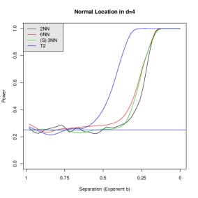
(a)

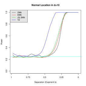
(b)

Figure 7. Empirical power in the normal location problem with $N_{1}=5000$ samples from $N(2\cdot\bm{1},\mathrm{I}_{d})$ and $N_{2}=3000$ samples from $N(2\cdot\bm{1}+N^{-b}\cdot\bm{h},\mathrm{I}_{d})$, where $b$ varies over a grid of 100 values in $[0,1]$, $\bm{h}=-\bm{1}$, and dimension (a) $d=4$ and (b) $d=10$.

Here, we provide additional simulations for testing local changes in the normal location family $\{N(\theta,\mathrm{I}_{d}):\theta\in\mathbb{R}^{d}\}$. Figure 7 shows the empirical power (out of 100 repetitions) of the different tests with $N_{1}=5000$ samples from $N(2\cdot\bm{1},\mathrm{I}_{d})$ and $N_{2}=3000$ samples from $N(2\cdot\bm{1}+N^{-b}\cdot\bm{h},\mathrm{I}_{d})$, where $b$ varies over a grid of 100 values in $[0,1]$, $\bm{h}=-\bm{1}$, and dimension (a) $d=4$ and (b) $d=10$. (Here, $N=N_{1}+N_{2}=8000$.) The level of the tests are set to $\alpha=0.25$. Note that the power of the tests based on the $K$-NN graphs transitions from $\alpha$ to 1 around $b=0.25$, which corresponds to the rate $N^{-\frac{1}{4}}$, as predicted by the calculations above. On the other hand, the power of the Hotelling’s $T^{2}$ test transitions from $\alpha$ to 1 around $b=0.5$, which corresponds to the parametric rate of $N^{-\frac{1}{2}}$. Note that these plots are qualitatively the same as those in Figure 4 in Section 4.2.1. This is because, for the normal location problem, the detection threshold does not depend on the dimension and the choice of the direction (recall discussion in Section 4.2.1).

F.2. The Spherical Normal Problem

In this section additional simulations for testing local changes in the spherical normal scale family $\{N(0,\sigma^{2}\mathrm{I}_{d}):\sigma>0\}$ are presented. Here, we zoom in to the different thresholds obtained in Theorem 4.2 and compare the power of the different tests.

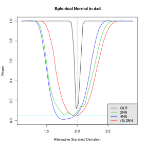
(a)

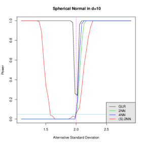
(b)

Figure 8. Empirical power for the spherical normal problem against $hN^{-\frac{1}{4}}$ alternatives, as a function of $h$, in dimension (a) $d=4$ and (b) $d=10$. The horizontal axis shows the scale parameter $\sigma$ under the alternative.

Figure 8 shows the empirical power (out of 100 repetitions) of the tests based on the 2-NN and 4-NN graphs, the test based on the symmetrized 2-NN graph, and the GLR test, with $N_{1}=10000$ samples from $N(0,2^{2}\cdot\mathrm{I}_{d})$ and $N_{2}=5000$ samples from $N(0,(2+hN^{-\frac{1}{4}})^{2}\mathrm{I}_{d})$, over a grid of 50 values of $h$ in $[-10,10]$ in (a) dimension 4 and (b) dimension 10. (Here, $N=N_{1}+N_{2}=15000$.) As before, in both cases, the GLR test has the highest power (going to 1). In dimension 4 (which is less than the critical dimension 8), the tests based on the NN graphs have non-trivial limiting local power as a function of $h$. However, in dimension 10 (Figure 8(b)), there is a drastic change in the shape of the limiting power curve:

$h>0$:

In this case, the power of all the tests quickly increase to 1 with increasing $h$. This is expected because, recalling the discussion in Section 4.2.2, for $d\geq 10$ and $h>0$, the detection threshold of the $K$-NN test is at $N^{-\frac{1}{2}+\frac{2}{d}}=N^{-\frac{3}{10}}\ll N^{-\frac{1}{4}}$, and the detection threshold of the GLR test is at $N^{-\frac{1}{2}}\ll N^{-\frac{1}{4}}$.

$h<0$:

Here, there is a region where the $K$-NN based tests have zero power, illustrating the non-monotonicity of the power function and the asymptotic biasedness phenomenon discussed in Section 4.2.2. This is because, in this case, the detection threshold is at $N^{-\frac{2}{d}}=N^{-\frac{1}{5}}\gg N^{-\frac{1}{4}}$.

To observe the emergence of these phase transitions more clearly, we now zoom in at the different thresholds with larger sample sizes. Hereafter, we set the level of tests to $\alpha=0.15$.

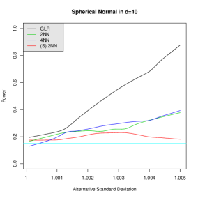
(a)

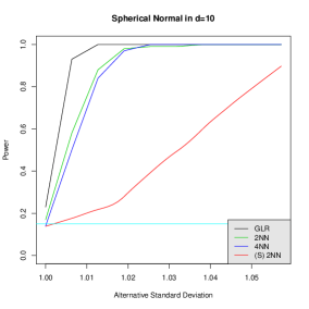
(b)

Figure 9. Empirical power for the spherical normal problem in dimension $d=10$ against (a) $hN^{-\frac{1}{2}}$ and (b) $hN^{-\frac{3}{10}}$ alternatives, as $h$ varies over a grid values in $[0,2]$. The horizontal axis shows the scale parameter $\sigma$ under the alternative.

$h>0$:

Figure 9 shows the empirical power (out of 100 repetitions) in dimension 10 of the different tests, with $N_{1}=80000$ samples from $N(0,\mathrm{I}_{d})$ and $N_{2}=60000$ samples from $N(0,(1+hN^{-b})^{2}\mathrm{I}_{d})$, over a grid of 10 values of $h$ in $[0,2]$. Figure 9(a) shows the case $b=0.5$ (which corresponds to parametric rate of detection). Here, as excepted, only the parametric GLR test has power increasing to 1. On the other hand, the power of the $K$-NN tests are significantly lower (closer to the level of the test). Note that the power of the 2-NN and the 4-NN tests do increase slightly with the number of neighbors $K$ and $h$, but this becomes less significant when the experiment is repeated with larger sample sizes (see the table in Figure 10(a)).

In Figure 9(b) we choose $b=0.3$, thus zooming in at the predicted detection threshold of $N^{-0.3}$, for $h>0$ (recall the discussion from Section 4.2.2). Here, the power of the $K$-NN tests quickly increase to 1. The same experiment, with $b=0.5$ and $b=0.3$, is repeated with larger sample sizes $N_{1}=400000$ and $N_{2}=300000$, and the results are presented in the tables in Figure 10, which further validate the theoretical findings.

$h$	0	0.5	1	1.5
2-NN	0.12	0.12	0.12	0.16
4-NN	0.16	0.2	0.22	0.24
2-(S)NN	0.12	0.14	0.12	0.16
GLR	0.13	0.21	0.49	0.61

(a) $\sigma=1+\frac{h}{N^{0.5}}$ under the alternative

$h$	0	0.5	1	1.5
2-NN	0.14	0.86	1	1
4-NN	0.08	1	1	1
2-(S)NN	0.24	0.26	0.44	0.8
GLR	0.22	1	1	1

(b) $\sigma=1+\frac{h}{N^{0.3}}$ under the alternative

Figure 10. Empirical power for the spherical normal problem in dimension $d=10$ for (a) $hN^{-\frac{1}{2}}$ and (b) $hN^{-\frac{3}{10}}$ alternatives, for varying $h$, with sample sizes $N_{1}=400000$ and $N_{2}=300000$.

$h<0$:

Figure 11 shows the empirical power in dimension 10 of the different tests, with $N_{1}=80000$ samples from $N(0,\mathrm{I}_{d})$ and $N_{2}=60000$ samples from $N(0,(1+hN^{-b})^{2}\mathrm{I}_{d})$, over a grid of 10 values of $h$ in $[0,2]$. Figure 11(a) zooms in at the parametric threshold ($b=0.5$), where only the GLR test has power increasing to 1, while the power of the $K$-NN tests remain close to the level (decreasing slightly with increasing $h$). In Figure 11(b) we take $b=\frac{1}{2}-\frac{2}{d}=0.3$, where the $K$-NN tests have power decreasing from the level 0.15 down to zero, as predicted by Theorem 4.2. In Figure 11(c) we zoom in at $N^{-0.2}$, that is, $b=\frac{2}{d}=0.2$. This is the detection threshold for the $K$-NN test for $h<0$, which we observe in the plots where the power sharply transitions from 0 to 1.

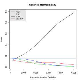
(a)

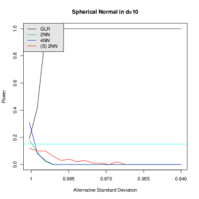
(b)

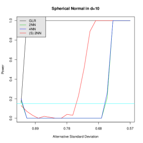
(c)

Figure 11. Empirical power for the spherical normal problem in dimension $d=10$ against (a) $hN^{-\frac{1}{2}}$, (b) $hN^{-\frac{3}{10}}$, and (c) $hN^{-\frac{1}{5}}$ alternatives, as a function of $h$. The horizontal axis shows the scale parameter $\sigma$ under the alternative.

References

- [1] D. Aldous, and J. M. Steele, Asymptotics for Euclidean minimal spanning trees on random points, Probab. Theory Related Fields, Vol. 92, 247–258, 1992.
- [2] E. Arias-Castro and B. Pelletier, On the consistency of the crossmatch test, Journal of Statistical Planning and Inference, 184–190, Vol. 171, 2016.
- [3] B. Aslan and G. Zech, New test for the multivariate two-sample problem based on the concept of minimum energy, Journal of Statistical Computation and Simulation, Vol. 75, 109–119, 2005.
- [4] L. Baringhaus and C. Franz, On a new multivariate two-sample test, Journal of Multivariate Analysis, Vol. 88, 190–206, 2004.
- [5] T. Batu, L. Fortnow, R. Rubinfeld, W. D. Smith, and P. White, Testing closeness of discrete distributions, Journal of the ACM, Vol. 60 (1), Article 4, 2013.
- [6] B. B. Bhattacharya, A general asymptotic framework for distribution-free graph-based two-sample tests, Journal of the Royal Statistical Society, Series B, Vol. 81 (3), 575–602, 2019.
- [7] P.J. Bickel, L. Breiman, Sums of functions of nearest neighbor distances, moment bounds, limit theorems and a goodness of fit test, Annals of Probability Vol. 11, 185–214, 1983.
- [8] S.-O. Chan, I. Diakonikolas, G. Valiant, and P. Valiant, Optimal algorithms for testing closeness of discrete distributions, Proc. Symposium on Discrete Algorithms (SODA), 1193–1203, 2014.
- [9] P. J. Bickel, A distribution free version of the Smirnov two sample test in the -variate case, Annals of Mathematical Statistics, Vol. 40, 1–23, 1969.
- [10] M. Biswas, M. Mukhopadhyay, A. K. Ghosh, A distribution-free two-sample run test applicable to high-dimensional data, Biometrika, Vol. 101(4), 913–926, 2014.
- [11] H. Chen and J. H. Friedman, A new graph-based two-sample test for multivariate and object data, J. Amer. Statist. Assoc. Vol. 112 (517), 397–409, 2017.
- [12] L. H. Y. Chen and Q.-M. Shao, Normal approximation under local dependence, Ann. Probab., Vol. 32 (3), 1985–2028, 2004.
- [13] B. Ebner, N. Henze, and J. Yukich, Multivariate goodness-of-fit on flat and curved spaces via nearest neighbor distances, Journal of Multivariate Analysis, Vol. 165, 231–242, 2018.
- [14] J. H. Friedman and L. C. Rafsky, Multivariate generalizations of the Wolfowitz and Smirnov two-sample tests, Ann. Statist., Vol. 7, 697–717, 1979.
- [15] A. Gretton, K. Borgwardt, M. Rasch, B. Scholkopf, and A. Smola, A kernel two-sample test, Journal of Machine Learning Research, Vol. 16, 723–773, 2012.
- [16] L. Györfi and T. Nemetz, -dissimilarity: A general class of separation measures of several probability measures, In Topics in Information Theory. Colloq. Math. Soc. János Bolyai, Vol. 16, 309–321, 1975.
- [17] P. Hall and N. Tajvidi, Permutation tests for equality of distributions in high-dimensional settings, Biometrika, Vol. 89, 359–374, 2002.
- [18] N. Henze, A multivariate two-sample test based on the number of nearest neighbor type coincidences, Ann. Statist., Vol. 16, 772–783, 1988.
- [19] N. Henze and M. D. Penrose, On the multivariate runs test, The Annals of Statistics, Vol. 27 (1), 290–298, 1999.
- [20] R. Y. Liu and K. Singh, A quality index based on data depth and multivariate rank tests, J. Amer. Statist. Assoc., Vol. 88, 252–260, 1993.
- [21] J.-F. Maa, D. K. Pearl, and R. Bartoszyński, Reducing multidimensional two-sample data to one-dimensional interpoint comparisons, The Annals of Statistics, Vol. 24 (3), 1069–1074, 1996.
- [22] H. B. Mann and D. R. Whitney, On a test of whether one of two random variables is stochastically larger than the other, Annals of Mathematical Statistics, Vol. 18(1), 50–60, 1947.
- [23] M. D. Penrose, Random Geometric Graphs, Oxford University Press, 2003.
- [24] M. D. Penrose, Gaussian limits for random geometric measures, Electronic Journal of Probability, Vol. 12, 989–1035, 2007.
- [25] M. D. Penrose and J. E. Yukich, Weak laws of large numbers in geometric probability, Ann. Appl. Probab. Vol. 13, 277–303, 2003.
- [26] P. R. Rosenbaum, An exact distribution-free test comparing two multivariate distributions based on adjacency, Journal of the Royal Statistical Society: Series B, Vol. 67 (4), 515–530, 2005.
- [27] V. Rousson, On distribution-free tests for the multivariate two-sample location-scale model, J. Mult. Anal., Vol. 80, 43–57, 2002.
- [28] W. Rudin, Real and Complex Analysis, 3rd ed. McGraw-Hill, New York, 1987.
- [29] M. F. Schilling, Multivariate two-sample tests based on nearest neighbors, J. Amer. Statist. Assoc., Vol. 81, 799–806, 1986.
- [30] N. Smirnoff, On the estimation of the discrepancy between empirical curves of distribution for two independent samples, Bulletin de Universite de Moscow, Serie internationale (Mathematiques), Vol. 2, 3–14, 1939.
- [31] J. W. Tukey, Mathematics and picturing data, In Proc. Intern. Congr. Math. Vancouver 1974, Vol. 2, 523–531, 1975.
- [32] A. Wald and J. Wolfowitz, On a test whether two samples are from the same distribution, Ann. Math. Statist., Vol. 11, 147–162, 1940.
- [33] L. Weiss, Two-sample tests for multivariate distributions, The Annals of Mathematical Statistics, Vol. 31, 159–164, 1960.
- [34] J. Yukich, Limit theorems in discrete stochastic geometry, Stochastic geometry, spatial statistics and random fields, Lecture Notes in Mathematics, 2068, 239–275, 2013.