Sparse preconditioning for model predictive control

Abstract

We propose fast $O(N)$ preconditioning, where $N$ is the number of gridpoints on the prediction horizon, for iterative solution of (non)-linear systems appearing in model predictive control methods such as forward-difference Newton-Krylov methods. The Continuation/GMRES method for nonlinear model predictive control, suggested by T. Ohtsuka in 2004, is a specific application of the Newton-Krylov method, which uses the GMRES iterative algorithm to solve a forward difference approximation of the optimality equations on every time step.

I Introduction

The paper deals with novel sparse preconditioning for model predictive control using, as a specific example, the Continuation/GMRES method for on-line nonlinear model predictive control suggested by T. Ohtsuka in [10]. The method becomes popular in solving industrial applications; see, e.g. [3]. The paper [7] gives guidelines how to use the method in cases, when the system dynamics obeys a geometric structure, e.g. the symplectic one, or when the state lies on a smooth manifold. The structure-preserving solver may increase accuracy of the numerical solution. The paper [8] treats the problems with the particle solutions for nonlinear MPC using Continuation/GMRES.

The Continuation/GMRES method is based on Newton-type optimization schemes. The exact Newton method requires an analytic expression of a corresponding Jacobian matrix, which is rarely available in practice and is often replaced with a forward difference (FD) approximation; see, e.g., [4]. Such approximate Newton-type optimization schemes utilize the FD approximation of the original nonlinear equation at every time step. T. Ohtsuka uses the GMRES algorithm to solve a finite-difference approximation $Ax=b$ to the optimality conditions. To cope with possible ill-conditioning of $A$, the authors of [15] propose a preconditioning strategy, which proved to be not very efficient.

In [5] and [6], we systematically search for better preconditioners to accelerate the GMRES and MINRES convergence in the C/GMRES method. In the present paper, we propose a sparse efficient $O(N)$ preconditioner for this method, where $N$ is the number of gridpoints on the prediction horizon.

Another popular approach to numerical solution of MPC problems is developed in [12], [13, 14], [16] and based on the interior-point method. The authors of [16] develop a direct method for a linear MPC model with the $O(N)$ arithmetic complexity. The papers [13, 14] apply the MINRES iteration with special preconditioners to similar linear MPC problems and prove the $O(N)$ arithmetical complexity of the preconditioned iteration. In contrast to the above methods, which use the Newton or quasi-Newton approximations, the recent papers [2] and [9] investigate performance of the first-order methods and their Nesterov’s acceleration.

Our proposed preconditioning technique is essentially based on two ideas. The symmetric matrix $A$ is a Schur complement of the Hessian of the Lagrangian function, associated with the model prediction problem. Apart from a few rows and columns, the preconditioner $M=LU$ is a sort of an incomplete LU factorization [1] of the Schur complement without these exceptional rows and columns. This results in sparse $M$ and its factors, $L$ and $U$, having only $O(N)$ nonzero entries. On the one hand, application of this preconditioner is almost as fast as that of a diagonal preconditioner. On the other hand, our preconditioner has high quality leading to fast convergence of the iterative method, such as GMRES.

The rest of the paper is organized as follows. Section II derives the nonlinear equation (11), which solves the model prediction problem, following [5, 10]. We prove the symmetry of the Jacobian matrix for the function defining (11) in Theorem 1. Section III describes the continuation method for solving (11). Section IV formulates the preconditioned GMRES, as in [5]. Section V describes our new preconditioner. The preconditioner construction is the main result of the paper. Section VI illustrates all details of the preconditioner setup on a representative example. Section VII displays plots of numerical results.

II Model prediction problem

The model predictive control (MPC) method solves a finite horizon prediction problem along a fictitious time $\tau\in[t,t+T]$. Our model finite horizon problem consists, following [5, 10], in choosing the control $u(\tau)$ and parameter vector $p$, which minimize the performance index $J$ as follows:

$$\min_{u,p}J,$$

where

$$J=\phi(x(\tau),p)|_{\tau=t+T}+\int_{t}^{t+T}L(\tau,x(\tau),u(\tau),p)d\tau$$

subject to the equation for the state dynamics

$$\frac{dx}{d\tau}=f(\tau,x(\tau),u(\tau),p),$$ (1)

and the constraints

$$C(\tau,x(\tau),u(\tau),p)=0,$$ (2)

$$\psi(x(\tau),p)|_{\tau=t+T}=0.$$ (3)

The initial value condition $x(\tau)|_{\tau=t}$ for (1) is the state vector $x(t)$ of the dynamic system. The control vector $u=u(\tau)$, solving the problem over the horizon, is used as an input to control the system at time $t$. The components of the vector $p(t)$ are parameters of the system. Equation (1) describes the system dynamic that may be nonlinear in $x$ and $u$. Equations (2) and (3) give equality constraints for the state $x$ and the control $u$. The horizon time length $T$ may in principle also depend on $t$.

The continuous formulation of the finite horizon problem stated above is discretized on a uniform, for simplicity of presentation, time grid over the horizon $[t,t+T]$ partitioned into $N$ time steps of size $\Delta\tau$, and the time-continuous vector functions $x(\tau)$ and $u(\tau)$ are replaced by their indexed values $x_{i}$ and $u_{i}$ at the grid points $\tau_{i}$, $i=0,1,\ldots,N$. The integral of the performance cost $J$ over the horizon is approximated by the rectangular quadrature rule. The time derivative of the state vector is approximated by the forward difference formula. The discretized optimal control problem is formulated as follows:

$$\min_{u_{i},p}\left[\phi(x_{N},p)+\sum_{i=0}^{N-1}L(\tau_{i},x_{i},u_{i},p)\Delta\tau\right],$$

subject to

$$\quad x_{i+1}=x_{i}+f(\tau_{i},x_{i},u_{i},p)\Delta\tau,\quad i=0,1,\ldots,N-1,$$ (4)

$$C(\tau_{i},x_{i},u_{i},p)=0,\quad i=0,1,\ldots,N-1,$$ (5)

$$\psi(x_{N},p)=0.$$ (6)

The necessary optimality conditions for the discretized finite horizon problem are obtained by means of the discrete Lagrangian function

$$\mathcal{L}(X,U)=\phi(x_{N},p)+\sum_{i=0}^{N-1}L(\tau_{i},x_{i},u_{i},p)\Delta\tau$$

$$+\,\lambda_{0}^{T}[x(t)-x_{0}]$$

$$+\sum_{i=0}^{N-1}\lambda_{i+1}^{T}[x_{i}-x_{i+1}+f(\tau_{i},x_{i},u_{i},p)\Delta\tau]$$

$$+\sum_{i=0}^{N-1}\mu_{i}^{T}C(\tau_{i},x_{i},u_{i},p)\Delta\tau+\nu^{T}\psi(x_{N},p),$$

where $X=[x_{i}\;\lambda_{i}]^{T}$, $i=0,1,\ldots,N$, and $U=[u_{i}\;\mu_{i}\;\nu\;p]^{T}$, $i=0,1,\ldots,N-1$. Here, $\lambda$ is the costate vector, $\mu$ is the Lagrange multiplier vector associated with the constraint (5). The terminal constraint (6) is relaxed by the aid of the Lagrange multiplier $\nu$. For further covenience, we also introduce the Hamiltonian function

$$H(t,x,\lambda,u,\mu,p)=L(t,x,u,p)$$

$${}+\lambda^{T}f(t,x,u,p)+\mu^{T}C(t,x,u,p).$$

The necessary optimality conditions are the (KKT) stationarity conditions: $\mathcal{L}_{\lambda_{i}}=0$, $\mathcal{L}_{x_{i}}=0$, $i=0,1,\ldots,N$, $\mathcal{L}_{u_{j}}=0$, $\mathcal{L}_{\mu_{j}}=0$, $i=0,1,\ldots,N-1$, $\mathcal{L}_{\nu_{k}}=0$, $\mathcal{L}_{p_{l}}=0$.

The KKT conditions are reformulated in terms of a mapping $F[U,x,t]$, where the vector $U$ combines the control input $u$, the Lagrange multiplier $\mu$, the Lagrange multiplier $\nu$, and the parameter $p$, all in one vector:

$$U(t)=[u_{0}^{T},\ldots,u_{N-1}^{T},\mu_{0}^{T},\ldots,\mu_{N-1}^{T},\nu^{T},p^{T}]^{T}.$$

The vector argument $x$ in $F[U,x,t]$ denotes the current measured or estimated state vector, which serves as the initial vector $x_{0}$ in the following procedure.

1. Starting from the current measured or estimated state $x_{0}$, compute $x_{i}$, $i=0,1\ldots,N-1$, by the forward recursion

   $$x_{i+1}=x_{i}+f(\tau_{i},x_{i},u_{i},p)\Delta\tau.$$

   Then starting from

   $$\lambda_{N}=\frac{\partial\phi^{T}}{\partial x}(x_{N},p)+\frac{\partial\psi^{T}}{\partial x}(x_{N},p)\nu$$

   compute the costates $\lambda_{i}$, $i=N,N\!-\!1,\ldots,1$, by the backward recursion

   $$\lambda_{i}=\lambda_{i+1}+\frac{\partial H^{T}}{\partial x}(\tau_{i},x_{i},\lambda_{i+1},u_{i},\mu_{i},p)\Delta\tau.$$

2. Calculate $F[U,x,t]$, using just obtained $x_{i}$ and $\lambda_{i}$, as

   $$F[U,x,t]$$

   $$=\left[\begin{array}[]{c}\begin{array}[]{c}\frac{\partial H^{T}}{\partial u}(\tau_{0},x_{0},\lambda_{1},u_{0},\mu_{0},p)\Delta\tau\\ \vdots\\ \frac{\partial H^{T}}{\partial u}(\tau_{i},x_{i},\lambda_{i+1},u_{i},\mu_{i},p)\Delta\tau\\ \vdots\\ \frac{\partial H^{T}}{\partial u}(\tau_{N-1},x_{N-1},\lambda_{N},u_{N-1},\mu_{N-1},p)\Delta\tau\end{array}\\ \\ \begin{array}[]{c}C(\tau_{0},x_{0},u_{0},p)\Delta\tau\\ \vdots\\ C(\tau_{i},x_{i},u_{i},p)\Delta\tau\\ \vdots\\ C(\tau_{N-1},x_{N-1},u_{N-1},p)\Delta\tau\end{array}\\ \\ \psi(x_{N},p)\\[8.61108pt] \begin{array}[]{c}\frac{\partial\phi^{T}}{\partial p}(x_{N},p)+\frac{\partial\psi^{T}}{\partial p}(x_{N},p)\nu\\ +\sum_{i=0}^{N-1}\frac{\partial H^{T}}{\partial p}(\tau_{i},x_{i},\lambda_{i+1},u_{i},\mu_{i},p)\Delta\tau\end{array}\end{array}\right].$$

The equation with respect to the unknown vector $U(t)$

$$F[U(t),x(t),t]=0$$ (11)

gives the required necessary optimality conditions.

Theorem 1

The Jacobian matrix $F_{U}[U,x,t]$ is symmetric for all $U$, $x$, and $t$.

Proof:

The equation $\mathcal{L}_{X}(X,U)=0$ is always solvable with respect to $X$ by the forward recursion for $x_{i}$ and backward recursion for $\lambda_{i}$. Let us denote its solution by $X=g(U)$. Then $F[U]=\mathcal{L}_{U}(g(U),U)$ and $F_{U}=\mathcal{L}_{UU}(g(U),U)+\mathcal{L}_{UX}(g(U),U)g_{U}$. Differentiation of the identity $\mathcal{L}_{U}(g(U),U)=0$ with respect to $U$ gives the identity $\mathcal{L}_{UU}(g(U),U)+\mathcal{L}_{UX}(g(U),U)g_{U}(U)=0$. Differentiation of the identity $\mathcal{L}_{X}(g(U),U)=0$ with respect to $U$ gives the identity $\mathcal{L}_{XU}(g(U),U)+\mathcal{L}_{XX}(g(U),U)g_{U}(U)=0$. Hence $g_{U}=-\mathcal{L}_{XX}^{-1}(g(U),U)\mathcal{L}_{XU}(g(U),U)$ and

$$F_{U}[U]= \mathcal{L}_{UU}(g(U),U)$$ (12)

$${}-\mathcal{L}_{UX}(g(U),U)\mathcal{L}_{XX}^{-1}(g(U),U)\mathcal{L}_{XU}(g(U),U),$$

which is the Schur complement of the symmetric Hessian matrix of $\mathcal{L}$ at the point $(X,U)=(g(U),U)$. The Schur complement of any symmetric matrix is symmetric. ∎

III Continuation algorithm

The controlled system is sampled on a uniform time grid $t_{j}=j\Delta t$, $j=0,1,\ldots$. Solution of equation (11) must be found at each time step $t_{j}$ on the controller board, which is a challenging part of implementation of NMPC.

Let us denote $x_{j}=x(t_{j})$, $U_{j}=U(t_{j})$, and rewrite the equation $F[U_{j},x_{j},t_{j}]=0$ equivalently in the form

$$F[U_{j},x_{j},t]-F[U_{j-1},x_{j},t_{j}]=b_{j},$$

where

$$b_{j}=-F[U_{j-1},x_{j},t_{j}].$$ (13)

Using a small $h$, which may be different from $\Delta t$ and $\Delta\tau$, we introduce the forward difference operator

$$a_{j}(V)=(F[U_{j-1}+hV,x_{j},t_{j}]-F[U_{j-1},x_{j},t_{j}])/h.$$ (14)

We note that the equation $F[U_{j},x_{j},t_{j}]=0$ is equivalent to the equation $a_{j}(\Delta U_{j}/h)=b_{j}/h$, where $\Delta U_{j}=U_{j}-U_{j-1}$.

Let us denote the $k$-th column of the $m\times m$ identity matrix by $e_{k}$, where $m$ is the dimension of the vector $U$, and define an $m\times m$ matrix $A_{j}$ with the columns $A_{j}e_{k}$, $k=1,\ldots,m$, given by the formula $A_{j}e_{k}=a_{j}(e_{k})$. The matrix $A_{j}$ is an $O(h)$ approximation of the Jacobian matrix $F_{U}[U_{j-1},x_{j},t_{j}]$. The Jacobian matrix $F_{U}$ is symmetric by Theorem 1.

Suppose that an approximate solution $U_{0}$ to the equation $F[U_{0},x_{0},t_{0}]=0$ is available. The first block entry of $U_{0}$ is then taken as the control $u_{0}$ at the state $x_{0}$. The next state $x_{1}=x(t_{1})$ is either sensor estimated or computed by the formula $x_{1}=x_{0}+f(t_{0},x_{0},u_{0})\Delta t$; cf. (1).

At the time $t_{j}$, $j>1$, we have the state $x_{j}$ and the vector $U_{j-1}$ from the previous time $t_{j-1}$. Our goal is to solve the following equation with respect to $V$:

$$a_{j}(V)=b_{j}/h.$$ (15)

Then we set $\Delta U_{j}=hV$, $U_{j}=U_{j-1}+\Delta U_{j}$ and choose the first block component of $U_{j}$ as the control $u_{j}$. The next system state $x_{j+1}=x(t_{j+1})$ is either sensor estimated or computed by the formula $x_{j+1}=x_{j}+f(t_{j},x_{j},u_{j})\Delta t$.

A direct way to solve (15) is generating the matrix $A_{j}$ and then solving the system of linear equations $A_{j}\Delta U_{j}=b_{j}$; e.g., by the Gaussian elimination.

A less expensive alternative is solving (15) by the GMRES method, where the operator $a_{j}(V)$ is used without explicit construction of the matrix $A_{j}$; cf., [4, 10].

IV Preconditioned GMRES

We recall that, for a given system of linear equations $Ax=b$ and initial approximation $x_{0}$, GMRES constructs orthonormal bases of the Krylov subspaces $\mathcal{K}_{n}=\text{span}\{r_{0},Ar_{0},\ldots,A^{n-1}r_{0}\}$, $n=1,2,\ldots$, given by the columns of matrices $Q_{n}$, such that $AQ_{n}=Q_{n+1}H_{n}$ with the upper Hessenberg matrices $H_{n}$ and then searches for approximations to the solution $x$ in the form $x_{n}=Q_{n}y_{n}$, where $y_{n}=\text{argmin}\|AQ_{n}y_{n}-b\|_{2}$.

The convergence of GMRES may stagnate for an ill-conditioned matrix $A$. The convergence can be improved by preconditioning. A matrix $M$ that is close to the matrix $A$ and such that computing $M^{-1}r$ for an arbitrary vector $r$ is relatively easy, is referred to as a preconditioner. The preconditioning for the system of linear equations $Ax=b$ with the preconditioner $M$ formally replaces the original system $Ax=b$ with the equivalent preconditioned linear system $M^{-1}Ax=M^{-1}b$. If the condition number $\|M^{-1}A\|\|A^{-1}M\|$ of the matrix $M^{-1}A$ is small, convergence of iterative solvers for the preconditioned system can be fast.

A typical implementation of the preconditioned GMRES is given by Algorithm 1. GMRES without preconditioning is the same algorithm with $z=r$. In the pseudocode, we denote by $H_{i_{1}:i_{2},j_{1}:j_{2}}$ the submatrix of $H$ with the entries $H_{ij}$ such that $i_{1}\leq i\leq i_{2}$ and $j_{1}\leq j\leq j_{2}$.

Algorithm 1 Preconditioned GMRES($k_{\max}$)

0:  $a(v)$, $b$, $x_{0}$, $k_{\max}$, $M$

0:  Solution $x$ of $a(x)=b$

1:  $r=b-a(x_{0})$, $z=M^{-1}r$, $\beta=\|z\|_{2}$, $v_{1}=z/\beta$

2:  for $k=1,\ldots,k_{\max}$ do

3:     $r=a(v_{k})$, $z=M^{-1}r$

4:     $H_{1:k,k}=[v_{1},\ldots,v_{k}]^{T}z$

5:     $z=z-[v_{1},\ldots,v_{k}]H_{1:k,k}$

6:     $H_{k+1,k}=\|z\|_{2}$

7:     $v_{k+1}=z/\|z\|_{2}$

8:  end for

9:  $y=\mbox{arg min}_{y}\|H_{1:k_{\max}+1,1:k_{\max}}y-[\beta,0,\dots,0]^{T}\|_{2}$

10:  $x=x_{0}+[v_{1},\ldots,v_{k_{\max}}]y$

It is a common practice to compute the LU factorization $M=LU$ by the Gaussian elimination and then compute the vector $M^{-1}r$ by the rule $M^{-1}r=U^{-1}(L^{-1}r)$.

V Sparse preconditioner

Our finite horizon model prediction problem allows us to construct sparse preconditioners $M_{j}$ with a particular structure. These preconditioners are highly efficient, which is confirmed by the numerical experiments described below.

We first observe that the states $x_{i}$, computed by the forward recursion, and the costates $\lambda_{i}$, computed by the subsequent backward recursion, satisfy, in practice, the following property: $\partial x_{i_{1}}/\partial u_{i_{2}}=O(\Delta\tau)$, $\partial\lambda_{i_{1}}/\partial u_{i_{2}}=O(\Delta\tau)$, $\partial x_{i_{1}}/\partial\mu_{i_{2}}=0$ and $\partial\lambda_{i_{1}}/\partial\mu_{i_{2}}=O(\Delta\tau)$. It is a corollary of theorems about the derivatives of solutions of ordinary differential equations with respect to a parameter; see, e.g., [11].

Now we assume that the predicted states $x_{i}$ and costates $\lambda_{i}$ are computed by the forward and backward recursions for the vector $U_{j-1}$ at the current system state $x_{j}=x(t_{j})$ during computation of the right-hand side vector $b_{j}$ and use the predicted $x_{i}$ and $\lambda_{i}$ to form the blocks $H_{uu}$, $H_{u\mu}$, $H_{\mu u}$, $H_{\mu\mu}$ of the symmetric matrix

$$M_{j}=\left[\begin{array}[]{ccc}H_{uu}(U_{j-1},x_{j},t_{j})&H_{u\mu}(U_{j-1},x_{j},t_{j})&M_{13}\\ H_{\mu u}(U_{j-1},x_{j},t_{j})&H_{\mu\mu}(U_{j-1},x_{j},t_{j})&M_{23}\\ M_{31}&M_{32}&M_{33}\end{array}\right],$$

where $[M_{31},M_{32},M_{33}]$ coincides with the last $l$ rows of $A_{j}$. The integer $l$ denotes the sum of dimensions of $\psi$ and $p$.

In the notation of Theorem 1, the above construction is explained as follows. We discard the second term in formula 12 and use the truncated expression $F_{U}[U]=\mathcal{L}_{UU}(g(U),U)$ for the entries of $M_{j}$ apart from the last $l$ columns and last $l$ rows. The last $l$ columns are computed exactly, the last $l$ rows equal the transposed last $l$ columns because of the symmetry of $M_{j}$. The possibility to use the truncated expression is due to the above observation that $\partial x_{i_{1}}/\partial u_{i_{2}}=O(\Delta\tau)$, $\partial\lambda_{i_{1}}/\partial u_{i_{2}}=O(\Delta\tau)$, $\partial x_{i_{1}}/\partial\mu_{i_{2}}=0$, $\partial\lambda_{i_{1}}/\partial\mu_{i_{2}}=O(\Delta\tau)$. Moreover, the norm of $A_{j}-M_{j}$ is of order $O(\Delta\tau)$.

The matrix $M_{j}$ is sparse since the blocks $H_{uu}$, $H_{u\mu}$, $H_{\mu u}$, $H_{\mu\mu}$ are block diagonal and $l$ is small. The particular structure of $M_{j}$ is convenient for efficient LU factorization. It is possible to simultaneously permute the rows and columns of $M_{j}$ and to obtain an arrow-like pattern of nonzero elements, which admits a fast LU factorization. A representative example of the sparse preconditioners $M_{j}$ and their LU factorization is given in the next section.

As a result, the setup of $M_{j}$, computation of its LU factorization, and application of the preconditioner all cost $O(N)$ floating point operations. The memory requirements are also of order $O(N)$.

VI Example

We consider a test nonlinear problem, which describes the minimum-time motion from a state $(x_{0},y_{0})$ to a state $(x_{f},y_{f})$ with an inequality constrained control:

• State vector $\vec{x}=\left[\begin{array}[]{c}x\\ y\end{array}\right]$ and input control $\vec{u}=\left[\begin{array}[]{c}u\\ u_{d}\end{array}\right]$.

• Parameter variables $\vec{p}=[t_{f}]$, where $t_{f}$ denotes the length of the evaluation horizon.

• Nonlinear dynamics is governed by the system of ODE

  $$\dot{\vec{x}}=f(\vec{x},\vec{u},\vec{p})=\left[\begin{array}[]{c}(Ax+B)\cos u\\ (Ax+B)\sin u\end{array}\right].$$

• Constraints: $C(\vec{x},\vec{u},\vec{p})=[(u-c_{u})^{2}+u_{d}^{2}-r_{u}^{2}]=0$, where $c_{u}=c_{0}+c_{1}\sin(\omega t)$, i.e., the control $u$ always stays within the curvilinear band $c_{u}-r_{u}\leq u\leq c_{u}+r_{u}$).

• Terminal constraints: $\psi(\vec{x},\vec{p})=\left[\begin{array}[]{c}x-x_{f}\\ y-y_{f}\end{array}\right]=0$ (the state should pass through the point $(x_{f},y_{f})$ at $t=t_{f}$)

• Objective function to minimize:

  $$J=\phi(\vec{x},\vec{p})+\int_{t}^{t+t_{f}}L(\vec{x},\vec{u},\vec{p})dt,$$

  where

  $$\phi(\vec{x},\vec{p})=t_{f},\quad L(\vec{x},\vec{u},\vec{p})=-w_{d}u_{d}$$

  (the state should arrive at $(x_{f},y_{f})$ in the shortest time; the function $L$ serves to stabilize the slack variable $u_{d}$)

• Constants: $A=B=1$, $x_{0}=y_{0}=0$, $x_{f}=y_{f}=1$, $c_{0}=0.8$, $c_{1}=0.3$, $\omega=20$, $r_{u}=0.2$, $w_{d}=0.005$.

The horizon $[t,t+t_{f}]$ is parameterized by the affine mapping $\tau\to t+\tau t_{f}$ with $\tau\in[0,1]$.

The components of the corresponding discretized problem on the horizon are given below:

• $\Delta\tau=1/N$, $\tau_{i}=i\Delta\tau$, $c_{ui}=c_{0}+c_{1}\sin(\omega(t+\tau_{i}p))$;

• the participating variables are the state $\left[\begin{array}[]{c}x_{i}\\ y_{i}\end{array}\right]$, the costate $\left[\begin{array}[]{c}\lambda_{1,i}\\ \lambda_{2,i}\end{array}\right]$, the control $\left[\begin{array}[]{c}u_{i}\\ u_{di}\end{array}\right]$, the Lagrange multipliers $\mu_{i}$ and $\left[\begin{array}[]{c}\nu_{1}\\ \nu_{2}\end{array}\right]$, the parameter $p$;

• the state is governed by the model equation

  $$\left\{\begin{array}[]{l}x_{i+1}=x_{i}+\Delta\tau\left[p\left(Ax_{i}+B\right)\cos u_{i}\right],\\ y_{i+1}=y_{i}+\Delta\tau\left[p\left(Ax_{i}+B\right)\sin u_{i}\right],\end{array}\right.$$

  where $i=0,1,\ldots,N-1$;

• the costate is determined by the backward recursion ($\lambda_{1,N}=\nu_{1}$, $\lambda_{2,N}=\nu_{2}$)

  $$\left\{\begin{array}[]{l}\lambda_{1,i}=\lambda_{1,i+1}\\ \hskip 25.00003pt{}+\Delta\tau\left[pA(\cos u_{i}\lambda_{1,i+1}+\sin u_{i}\lambda_{2,i+1})\right],\\ \lambda_{2,i}=\lambda_{2,i+1},\end{array}\right.$$

  where $i=N-1,N-2,\ldots,0$;

• the equation $F(U,x_{0},y_{0},t)=0$, where

  $$U=[u_{0},u_{d,0},\ldots,u_{N-1},u_{d,N-1},$$

  $$\mu_{0},\ldots,\mu_{N-1},\nu_{1},\nu_{2},p],$$

  has the following rows from the top to bottom:

  $$\left\{\begin{array}[]{l}\Delta\tau\left[p(Ax_{i}+B)\left(-\sin u_{i}\lambda_{1,i+1}+\cos u_{i}\lambda_{2,i+1}\right)\right.\\ \hskip 110.00017pt\left.{}+2\left(u_{i}-c_{ui}\right)\mu_{i}\right]=0\\ \Delta\tau\left[2\mu_{i}u_{di}-w_{d}p\right]=0\end{array}\right.$$

  $$\left\{\Delta\tau\left[(u_{i}-c_{ui})^{2}+u_{di}^{2}-r_{u}^{2}\right]=0\right.\hskip 70.0001pt$$

  $$\left\{\begin{array}[]{l}x_{N}-x_{r}=0\\ y_{N}-y_{r}=0\end{array}\right.\hskip 150.00023pt$$

  $$\left\{\begin{array}[]{l}\Delta\tau[\sum\limits^{N-1}_{i=0}(Ax_{i}+B)(\cos u_{i}\lambda_{1,i+1}+\sin u_{i}\lambda_{2,i+1})\\ \hskip 10.00002pt{}-2(u_{i}-c_{ui})\mu_{i}c_{1}\cos(\omega(t+\tau_{i}p))\omega\tau_{i}\\ \hskip 80.00012pt-w_{d}u_{di}]+1=0.\end{array}\right.$$

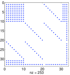
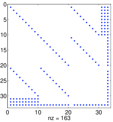
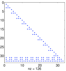
The matrices $A_{j}$ have the sparsity structure as in Fig. 4. The preconditioner $M_{j}$ is the symmetric matrix

$$M_{j}=\left[\begin{array}[]{ccccc}M_{11}&0&M_{13}&M_{14}&M_{15}\\ 0&M_{22}&M_{23}&0&M_{25}\\ M_{31}&M_{32}&0&0&M_{35}\\ M_{41}&0&0&0&M_{45}\\ M_{51}&M_{52}&M_{53}&M_{45}&M_{55}\end{array}\right]$$

having the diagonal blocks $M_{11}$, $M_{13}=M_{31}^{T}$, $M_{22}$, $M_{23}=M_{32}^{T}$. The diagonal entries of $M_{11}$ equal $\Delta\tau[2\mu_{i}-p(Ax_{i}+B)(\cos u_{i}\lambda_{1,i+1}+\sin u_{i}\lambda_{2,i+1})]$. The diagonal entries of $M_{22}$ equal $\Delta\tau 2\mu_{i}$. The diagonal entries of $M_{13}$ equal $\Delta\tau 2(u_{i}-c_{ui})$. The diagonal entries of $M_{23}$ equal $\Delta\tau 2u_{di}$. The entries of the vector $M_{15}$ equal $\Delta\tau(Ax_{i}+B)(-\sin u_{i}\lambda_{1,i+1}+\cos u_{i}\lambda_{2,i+1})-\Delta\tau 2\mu_{i}c_{1}\cos(\omega(t+\tau_{i}p))\omega\tau_{i}$. The entries of the vector $M_{25}$ equal $-\Delta\tau w_{d}$. The entries of the vector $M_{35}$ equal $-2\Delta\tau(u_{i}-c_{ui})c_{1}\cos(\omega(t+\tau_{i}p))\omega\tau_{i}$.

The blocks $M_{14}$, $M_{45}$, and $M_{55}$ equal to the respective blocks of $A$ and have to be computed exactly. The sparsity pattern of $M_{j}$ is displayed in Fig. 4.

To compute the LU factorization of $M_{j}$ with $O(N)$ floating point operations, we first repartition $M_{j}$ as

$$M_{j}=\left[\begin{array}[]{ccccc}K_{11}&K_{12}\\ K_{21}&K_{22}\end{array}\right],K_{11}=\left[\begin{array}[]{ccccc}M_{11}&0&M_{13}\\ 0&M_{22}&M_{23}\\ M_{31}&M_{32}&0\end{array}\right],$$

where $K_{11}$ is usually nonsingular. Using the representation

$$K_{11}^{-1}=\left[\begin{array}[]{rrr}M_{23}M_{32}&-M_{13}M_{32}&M_{13}M_{22}\\ -M_{23}M_{31}&M_{13}M_{31}&M_{11}M_{23}\\ M_{22}M_{31}&M_{11}M_{32}&-M_{11}M_{22}\end{array}\right]\\$$

$$\times\left[\begin{array}[]{rrr}D\\ &D\\ &&D\end{array}\right],$$

where $D=(M_{11}M_{23}M_{32}+M_{13}M_{22}M_{31})^{-1}$, we obtain the block triangular factors

$$L=\left[\begin{array}[]{cc}I&0\\ K_{21}K^{-1}_{11}&I\end{array}\right],\;U=\left[\begin{array}[]{cc}K_{11}&K_{12}\\ 0&S_{22}\end{array}\right],$$

where $S_{22}=K_{22}-K_{21}K_{11}^{-1}K_{12}$. The application of the preconditioner costs $O(N)$ operations.

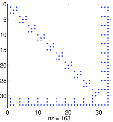
An alternative construction of the LU factorization uses a suitable simultaneous permutation of the rows and columns of $M_{j}$ with the permutation indices $1,1+N,1+2N$,…, $i,i+N,i+2N$,…,$N,2N,3N,1+3N,2+3N,3+3N$. The sparsity patterns of the permuted matrix and its lower triangular factor $L$ are displayed in Fig. 5, the sparsity pattern of the upper triangular factor $U$ is the transpose of that of the factor $L$.

VII Numerical results

In our numerical experiments, carried out in MATLAB, the system of weakly nonlinear equations (15) for the test problem from Section VI is solved by the GMRES method. The error tolerance in GMRES is $tol=10^{-5}$. The number of grid points on the horizon is $N=100$, the sampling time of the simulation is $\Delta t=1/500$, and $h=10^{-8}$.

The sparse preconditioners for GMRES are constructed as in Section VI, and the LU factorization is computed as proposed in the last paragraph of Section VI.

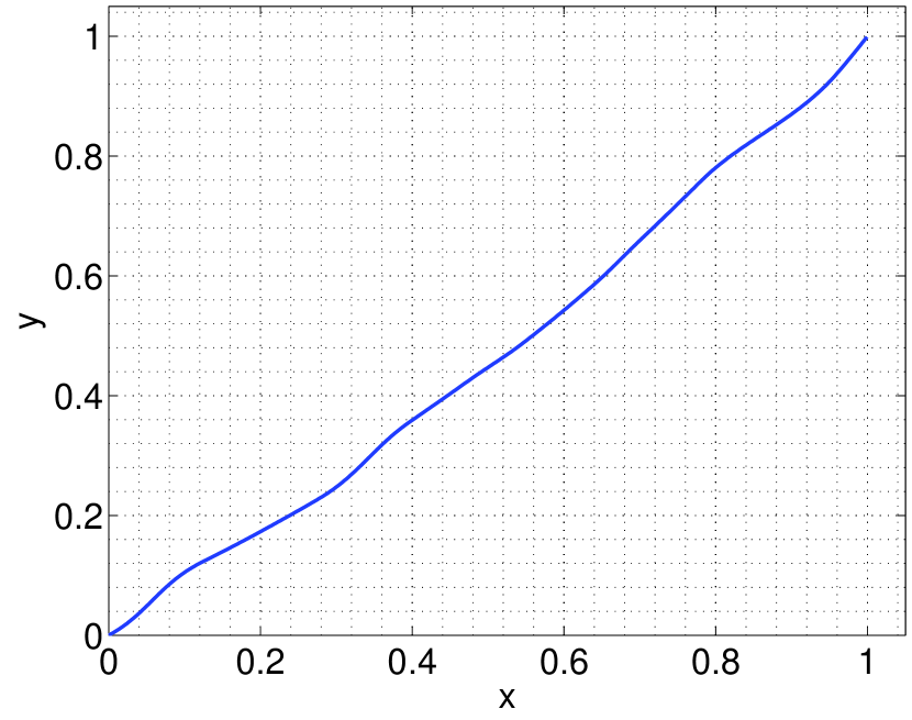
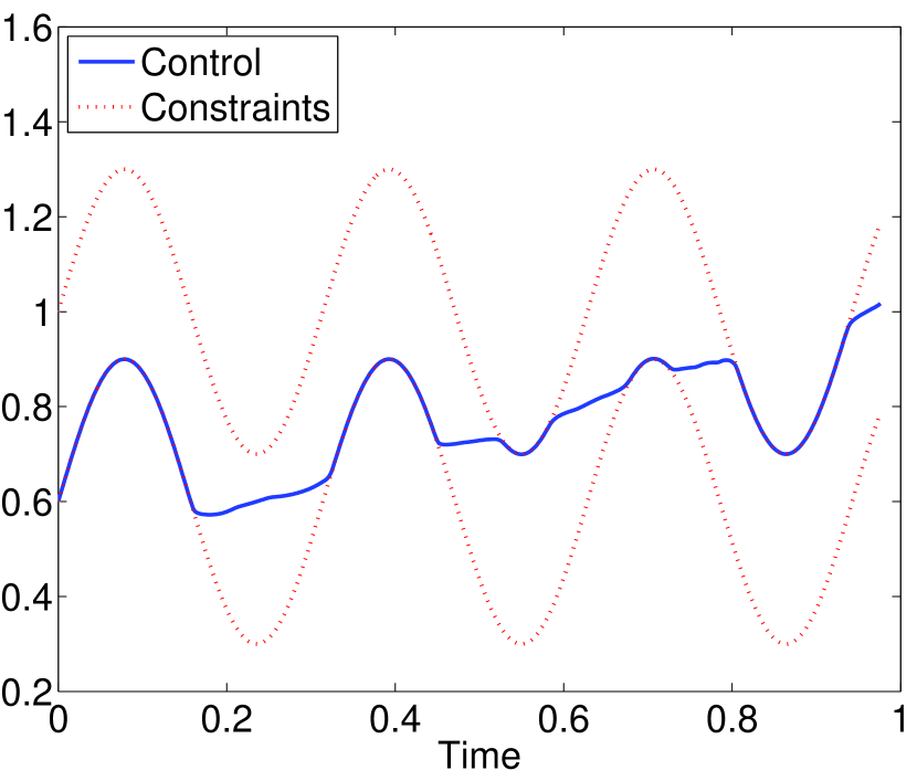
Figure 1 shows the computed trajectory for the test example and Figure 2 shows the optimal control by the MPC approach using GMRES with preconditioning.

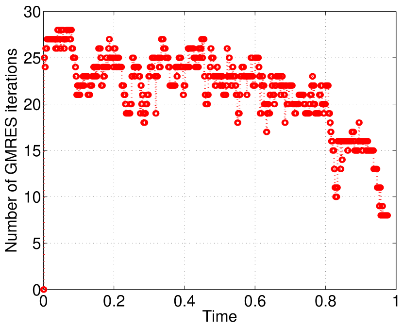
GMRES with preconditioning executes only 2 iterations at each step while keeping $\|F\|_{2}$ close to $10^{-4}$. For comparison, we show the number of iterations in GMRES without preconditioning in Figure 3, which is 4-14 times larger.

Figure 1: Trajectory by NPMC using GMRES with preconditioning

Figure 2: NMPC control $u$ using GMRES with preconditioning

Figure 3: The number of GMRES iterations without preconditioning, $N=100$, $\Delta t=1/500$, $k_{\max}=100$

Figure 4: Sparsity patterns of the Jacobian $F_{U}$ and preconditioner $M$

Figure 5: Sparsity patterns of the permuted preconditioner and the lower triangular factor $L$

VIII Conclusion

We propose an efficient sparse preconditioner for the Continuation/GMRES method for nonlinear MPC problems. The arithmetical cost of preconditioning is $O(N)$, memory storage is $O(N)$, where $N$ is the number of gridpoints on the prediction horizon.

References

• [1] O. Axelsson, Iterative solution methods. New York, NY: Cambridge U. Press, 1994.
• [2] P. Giselsson, Optimal preconditioning and iteration complexity bounds for gradient-based optimization in model predictive control, in Proc. American Control Conf., Washington D.C., USA, June, 2013, pp. 358–364.
• [3] M. Huang, H. Nakada, K. R. Butts, and I. V. Kolmanovsky, Nonlinear Model Predictive Control of a Diesel Engine Air Path: A Comparison of Constraint Handling and Computational Strategies, in Proc. 5th IFAC Conf. Nonlinear Model Predictive Control, Seville, Spain, September 17–20, 2015, pp. 372–379.
• [4] C. T. Kelly, Iterative methods for linear and nonlinear equations. Philadelphia, PA: SIAM, 1995.
• [5] A. Knyazev, Y. Fujii, and A. Malyshev, Preconditioned Continuation Model Predictive Control, in Proc. SIAM Conf. Control Appl., Paris, France, July 8–10, 2015, pp. 101–108.
• [6] A. Knyazev and A. Malyshev, Preconditioning for Continuation Model Predictive Control, in Proc. 5th IFAC Conf. Nonlinear Model Predictive Control, Seville, Spain, September 17–20, 2015, pp. 191–196. Available at arXiv:1509.02861.
• [7] A. Knyazev and A. Malyshev, Continuation model predictive control on smooth manifolds, in Proc. 16th IFAC Workshop Control Applications of Optimization, Garmisch-Partenkirchen, Germany, October 6–9, 2015. Available at arXiv:1509.02848.
• [8] A. Knyazev and A. Malyshev, Efficient particle continuation model predictive control, in Proc. 16th IFAC Workshop Control Applications of Optimization, Garmisch-Partenkirchen, Germany, October 6–9, 2015. Available at arXiv:1509.02852.
• [9] D. Kouzoupis, H. J. Ferreau, H. Peyrl, and M. Diehl, First-order methods in embedded nonlinear model predictive control, in Proc. European Control Conf., Linz, Austria, 2015, pp. 2622–2627.
• [10] T. Ohtsuka, A Continuation/GMRES method for fast computation of nonlinear receding horizon control, Automatica, vol. 40, pp. 563–574, 2004.
• [11] L. S. Pontryagin, Ordinary differential equations. Reading, MA: Addison-Wesley, 1962.
• [12] C. V. Rao, S. J. Wright, and J. B. Rawlings, Application of interior-point methods to model predictive control, J. Optimiz. Theory Appl., vol. 99, pp. 723–757, 1998.
• [13] A. Shahzad, E. C. Kerrigan, and G. A. Constantinides, Preconditioners for Inexact Interior Point Methods for Predictive Control, in Proc. American Control Conf., Baltimore, MD, USA, June 30–July 2, 2010, pp. 5714–5719.
• [14] A. Shahzad, E. C. Kerrigan, and G. A. Constantinides, A Fast Well-conditionend Interior Point Method for Predictive Control, in Proc. IEEE Conf. Decision Control, Atlanta, GA, USA, December 15–17, 2010, pp. 508–513.
• [15] T. Tanida and T. Ohtsuka, Preconditioned C/GMRES algorithm for nonlinear receding horizon control of hovercrafts connected by a string, in Proc. IEEE Int. Conf. Control Appl., Taipei, Taiwan, September 2-4, 2004, pp. 1609–1614.
• [16] Y. Wang and S. Boyd, Fast model predictive control using online optimization, IEEE Trans. Control Syst. Technology, vol. 18, pp. 267–278, 2010.