The gradient flow in simple field theories

Abstract:

The gradient flow is a valuable tool for the lattice community, with applications from scale-setting to implementing chiral fermions. Here I focus on the gradient flow as a means to suppress power-divergent mixing. Power-divergent mixing stems from the hypercubic symmetry of the lattice regulator and is a particular difficulty for calculations of, for example, high moments of parton distribution functions. The gradient flow removes power-divergent mixing on the lattice, provided the flow time is kept fixed in physical units, at the expense of introducing a new physical scale in the continuum. One approach to dealing with this new scale is the smeared operator product expansion, a formalism that systematically connects nonperturbative calculations of flowed operators to continuum physics. I study the role of the gradient flow in suppressing power-divergent mixing and present the first nonperturbative study in scalar field theory.

1 Introduction

The curse of power-divergent mixing afflicts a range of lattice calculations, but the prototypical example occurs in calculations of matrix elements of twist-2 operators, where twist is the dimension minus the spin of the operator. These matrix elements arise, for example, in lattice determinations of moments of parton distribution functions, which capture the distribution of a fast-moving nucleon’s longitudinal momentum amongst its constituents. For twist-2 operators, power-divergent mixing stems from the hypercubic symmetry of the lattice regulator.

In general, the symmetry restrictions of the finite hypercubic group are less stringent than those imposed by the orthogonal group of continuous Euclidean spacetime and allow for more complicated radiative mixing. Operators of definite angular momentum, for example, do not mix in the continuum. The lattice regulator breaks rotational symmetry, however, and angular momentum is no longer a good quantum number in a discretised spacetime. Lattice operators that correspond to a state with definite angular momentum in the continuum may therefore mix. For operators of different mass dimension, this mixing generates contributions that diverge as an inverse power of the lattice spacing in the continuum limit: the problem of power-divergent mixing. Such contributions must be removed to extract meaningful continuum physics.

In [1], we introduced a modified operator product expansion–the smeared operator product expansion–to remove power-divergent mixing via the gradient flow. The gradient flow, a gauge-invariant form of smearing with particularly useful renormalisation properties [2], drives the original degrees of freedom to the stationary points of the action and corresponds to a continuous stout-smearing procedure [3]. Smearing has long been used in lattice calculations to reduce discretisation effects and improve the continuum limit of lattice data. There is a history, too, of modifying the operator product expansion on the lattice to account for power-divergent mixing [4], although these techniques have not been widely adopted. Here I discuss the use of the gradient flow to remove power-divergent mixing and consider some examples in scalar field theory.

2 The smeared operator product expansion

The operator product expansion (OPE) for a non-local operator in scalar field theory is widely-known (see, for example, [5]), so here I just introduce some necessary notation. I write the OPE for a non-local operator, ${\cal Q}(x)$, as

$${\cal Q}(x)\stackrel{{\scriptstyle x\rightarrow 0}}{{\sim}}\;\sum_{k}c_{k}(x,\mu){\cal O}_{R}^{(k)}(0,\mu).$$ (1)

The $c_{k}(x,\mu)$ are perturbative Wilson coefficients that capture the short-distance physics associated with the renormalised local operator ${\cal O}_{R}^{(k)}(0,\mu)$, where $\mu$ is the renormalisation scale. This operator is a polynomial in the scalar field and its derivatives, and the operator’s free-field mass dimension governs the leading spacetime dependence of the Wilson coefficients. Radiative corrections generate sub-leading dependence on the spacetime separation. The Wilson coefficients are functions of the spacetime separation $x$; the (renormalised) mass $m$; and the renormalisation scale, $\mu$. Here, one should interpret this equality in the weak sense of holding between matrix elements.

In [1] we proposed a new expansion in terms of smeared operators, the smeared OPE:

$${\cal Q}(x)\stackrel{{\scriptstyle x\rightarrow 0}}{{\sim}}\;\sum_{k}d_{k}(\tau,x,\mu){\cal S}_{R}^{(k)}(\tau,0,\mu).$$ (2)

The smeared coefficients $d_{k}(\tau,x,\mu)$ are now functions of three scales: the smearing scale, $\tau$; the spacetime separation, $x$; and the renormalisation scale, $\mu$. The smeared operator, ${\cal S}_{R}(\tau,0)$, has the same free-field mass dimension as its local counterpart. Thus, the smeared coefficients exhibit the same leading spacetime dependence as that of the local Wilson coefficients.

Although we referred to these operators as generically “smeared”, one should recognise that we had in mind a particular form of smearing: the gradient flow [2, 6]. The gradient flow is a classical evolution of the original degrees of freedom towards the stationary points of the action in a new dimension, the flow time, with the particularly useful property that renormalised correlation functions remain renormalised at non-zero flow time (up to a fermion renormalisation) [2].

Working with scalar field theory in two dimensions, defined by the action

$$S_{\phi}[\phi]=\frac{1}{2}\int\mathrm{d}^{2}x\,\left[(\partial_{\nu}\phi)^{2}+m_{\phi}^{2}\phi^{2}+\frac{\lambda_{\phi}}{2}\phi^{4}\right],$$ (3)

the flow time evolution takes a particularly simple form (see [7] for a rather different application of the gradient flow that also takes advantage of its simplicity):

$$\frac{\partial\rho(\tau,x)}{\partial\tau}=\partial^{2}\rho(\tau,x).$$ (4)

Here $\partial^{2}$ is the Euclidean Laplacian operator. Imposing the Dirichlet boundary condition $\rho(0,x)=\phi(x)$, one can solve this equation exactly. The solution is

$$\rho(\tau,x)=\frac{1}{4\pi\tau}\int\mathrm{d}^{2}y\,e^{-(x-y)^{2}/4\tau}\phi_{2}(y),$$ (5)

which demonstrates explicitly the “smearing” effect of the gradient flow: the flow time exponentially damps ultraviolet fluctuations. The root-mean-square smearing length, which is $s_{\mathrm{rms}}=2\sqrt{\tau}$ in two dimensions, characterises the corresponding smearing radius.

The flow evolution equation, Equation (4), is straightforward and manifestly corresponds to Gaussian-smearing of the scalar degrees of freedom. In principle, however, we are free to choose the precise form of the flow time evolution equation (provided it drives the fields to configurations corresponding to minima of the action), and we could incorporate interactions in the flow time evolution, as is done in QCD and the nonlinear sigma model. This choice would, unfortunately, remove the renormalisation property of the gradient flow that proves so useful: renormalised correlation functions would no longer be guaranteed to remain finite at non-zero flow time. Ultimately this result stems from the internal symmetries of QCD and the nonlinear sigma model that have no analogue in scalar $\phi^{4}$ theory. In pure Yang-Mills theory and the nonlinear sigma model, it is gauge invariance, manifest through appropriate BRST symmetries, that ensures no new counterterms can be generated by the gradient flow [2].

3 Nonperturbative scalar field theory

I study two-dimensional $\phi^{4}$ theory on small ($N=L/a=16,32$) to medium-sized square lattices ($N=128,256$). The lattice action is

$$S_{\phi}^{\mathrm{latt}}[\phi]=\sum_{n}\left[-\sum_{i=1}^{2}\phi(n+i)\phi(n)+\left(2+\frac{m_{0}^{2}}{2}\right)\phi^{2}(n)+\frac{\lambda}{4}\phi^{4}(n)\right],$$ (6)

where the sum runs over all lattice sites $n$ in the lattice volume $N^{2}=(L/a)^{2}$ and $m_{0}=am_{\phi}$ is the dimensionless bare mass. The lattice coupling constant $\lambda=a^{2}\lambda_{\phi}$ is also dimensionless. In the infinite volume limit, this theory has a continuous phase transition between the symmetric phase, in which $\langle\phi\rangle=0$, and a broken phase, in which $\langle\phi\rangle\neq 0$, explored in, for example, [8]. The continuum limit corresponds to the origin in the bare lattice mass-coupling plane and is parameterised by a single dimensionless number.

In two dimensions, $\phi^{4}$ theory is super-renormalisable [8]; there is a single divergent tadpole diagram, which is given by

$$A_{m_{0}^{2}}^{\mathrm{latt}}=\frac{1}{N^{2}}\sum_{k=0}^{N-1}\frac{1}{4\sin^{2}(\pi k/N)+m^{2}}\;\stackrel{{\scriptstyle[}}{{m}}\,\mathrm{fixed}]{N\rightarrow\infty}{=}\;\int_{0}^{\infty}\mathrm{d}u\,e^{-u(4-m^{2})}[I_{0}(2u)]^{2},$$ (7)

where the second equality holds in the infinite volume limit, $I_{0}(z)$ is the modified Bessel function of the first kind, and $m$ is the renormalised (lattice) mass. Perturbatively, the renormalisation condition $\delta m^{2}=3\lambda A_{m^{2}}$ removes all ultraviolet divergences. In principle one could choose to define a renormalised coupling, either through the four-point function or with a finite volume scheme based on the gradient flow, analogous to that proposed in [9], but this is unnecessary, because the renormalised coupling differs by a finite shift from the bare coupling.

Numerical tests

To combat critical slowing down, I use a Monte Carlo procedure that incorporated five Metropolis update steps followed by an embedded Wolff cluster update step [10] (there also exist microcanonical and multigrid methods for this system [11]). I thermalised the lattices for at least $10^{4}$ such “sweeps” and took measurements every 100 sweeps to reduce autocorrelations (at the critical mass, for example, I found integrated autocorrelation times up to approximately 80 update steps for $\langle\phi^{2}\rangle$, in line with [8]).

I plot the integrated autocorrelation times $\tau_{\mathrm{int}}$, calculated using the Gamma analysis of [12], for $\langle\phi^{2}\rangle$ with simple Metropolis updating in the left-hand panels of Figure 1 and for Metropolis steps combined with a embedded cluster update step in the right-hand panels of the same figure (for details, see the corresponding caption). In general, including the cluster update improves the integrated autocorrelation time by a factor of two to three. The increased integrated autocorrelation time at $m_{0}^{2}=-0.72$ indicates the critical slowing down associated with a phase transition.

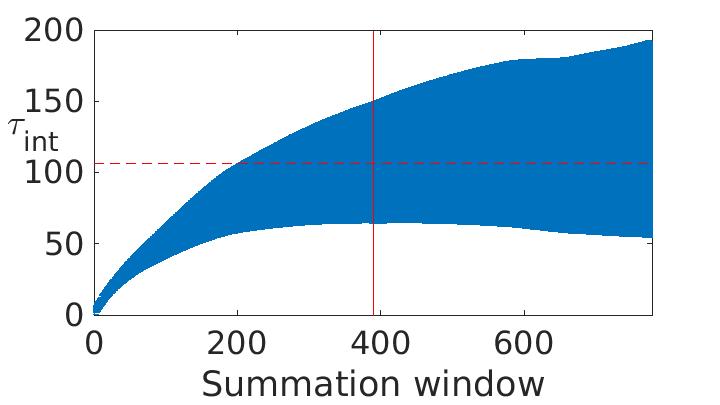
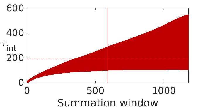
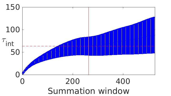
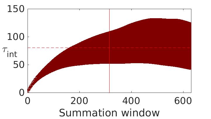
Figure 1: The autocorrelation time for $\langle\phi^{2}\rangle$, as a function of the summation window of the Gamma analysis of [12]. Simple Metropolis updating at: (far left) $m_{0}^{2}=-0.68$ and (centre left) $m_{0}^{2}=-0.72$. Metropolis algorithm with an embedded cluster update step at: (centre right) $m_{0}^{2}=-0.68$ and (far right) $m_{0}^{2}=-0.72$. All plots show data for $N=64$ and $\lambda=0.5$. The vertical red lines represent the value of the summation window automatically chosen by the Gamma analysis procedure and the horizontal red lines give the corresponding integrated autocorrelation time.

I illustrate the existence of the phase transition, which occurs at $m_{0}^{2}=-0.72$ for $\lambda=0.5$ and at $m_{0}^{2}=-1.27$ for $\lambda=1.0$, in Figure 2. In the left-hand panels, I plot the distributions of the values of $\phi$ from a single lattice at two points in the mass-coupling parameter space. These points correspond to the symmetric (far left) and broken (centre left) phases in the infinite volume limit. The histograms demonstrate that, as the lattice size increases, the distribution of $\phi$ values collapses to a Gaussian distribution centred on zero for $m_{0}^{2}=-0.64$, corresponding to the symmetric phase, and a Gaussian centred around $\langle\phi\rangle\neq 0$ for $m_{0}^{2}=-0.72$, corresponding to the broken phase.

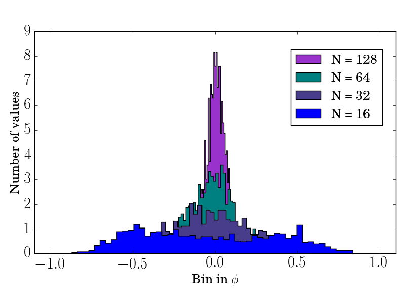
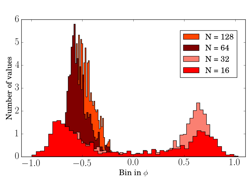
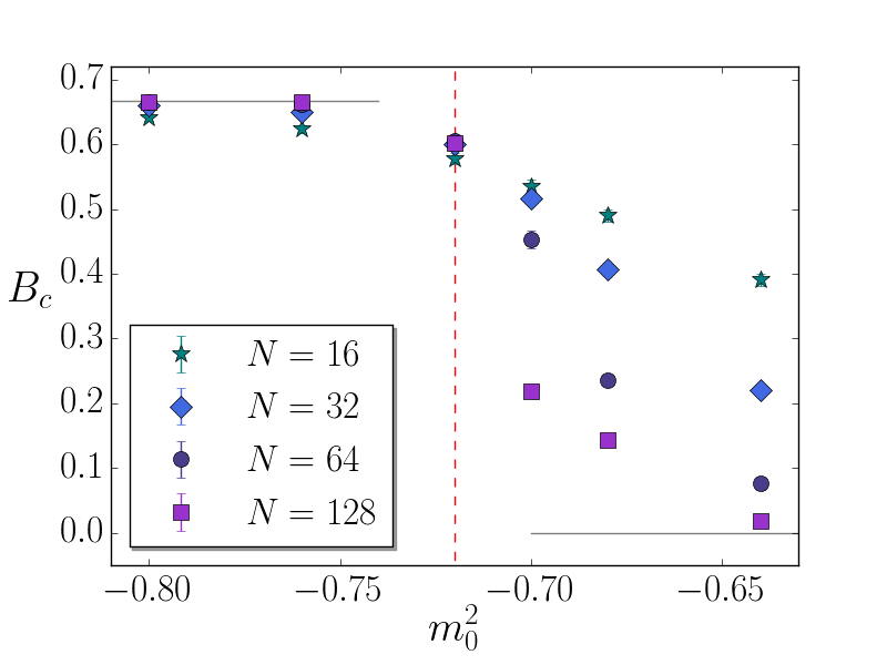
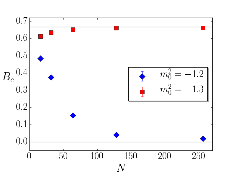
Figure 2: Testing the two phases: (Left panels) Histograms representing the distribution of $\phi$ values on a single lattice in two regions corresponding to (far left) the symmetric phase ($am_{0}^{2}=-0.64$, $\lambda=0.5$) and (centre left) the broken phase ($am_{0}^{2}=-0.72$, $\lambda=0.5$), in the infinite volume limit. (Right panels) The Binder cumulant, $B_{c}$, as a function of (centre right) the bare mass, $m_{0}^{2}$, at $\lambda=0.5$ and for different lattice volumes, and (far right) as a function of lattice size, at fixed bare mass and coupling constant. The horizontal grey lines correspond to the infinite volume values in the symmetric and broken phases: $B_{c}=0$ and $B_{c}=2/3$, respectively. The vertical red dashed line in the left-hand plot corresponds to the critical mass. Uncertainties are smaller than the size of the data point markers. Data from 10⁴ measurements.

As a further test, I studied the fourth-order Binder cumulant, $B_{c}$, an order parameter for the phase transition from the symmetric to the broken phase. This cumulant is defined as $B_{c}=1-\overline{\phi^{4}}/3(\overline{\phi^{2}})^{2}$, where $\overline{\phi}$ is the volume-averaged value of $\phi$ on a single configuration [Binder:1981ul]. In the infinite volume limit, $B_{c}=0$ in the symmetric phase and $B_{c}=2/3$ in the broken phase. In the right-hand panels of Figure 2 I plot: (centre right) the Binder cumulant as a function of the bare lattice mass $m_{0}^{2}$, at fixed coupling constant $\lambda=0.5$ and for different lattice sizes; and (far right) as a function of lattice size for three different bare lattice masses at fixed coupling $\lambda=1.0$. These plots demonstrate that, in the infinite volume limit, the Binder cumulant tends to the correct value in both phases.

Mixing and the gradient flow

Let us consider the matrix element $\left\langle\Omega|\phi^{2}(0)\cdot\phi(0)\partial^{2}\phi(0)|\Omega\right\rangle$ in perturbation theory [1]. In the continuum this matrix element vanishes. On the lattice, however, the corresponding matrix element in four dimensions diverges with the inverse lattice spacing squared, signaling the appearance of power-divergent mixing. In the continuum limit, keeping the flow time $\tau$ fixed in physical units, this matrix element tends to a constant, signaling the suppression of power-divergent mixing for smeared degrees of freedom. Note, however, that we have not removed mixing entirely, but only suppressed the problematic power-divergent mixing. In two dimensions, the lattice matrix element diverges only logarithmically with the cutoff, but the principle remains the same: fixing the flow time removes this divergent behaviour.

We see this in Figure 3. In the left-hand panel I plot the vacuum expectation value of $\phi^{2}(0)\cdot\phi(0)\nabla^{2}\phi(0)$ in the symmetric phase, as a function of the bare mass $m_{0}^{2}$ (expressed as a ratio to the critical mass, $m_{\mathrm{crit}}^{2}$). The true continuum limit corresponds to the origin in the bare mass-coupling plane, but for our purposes we can consider instead the approach to the critical point at fixed coupling. I extrapolate to the infinite volume limit with a polynomial fit to $1/N$, including terms up to $1/N^{3}$, for lattices from $N=16$ to $N=256$. The magenta band corresponds to a fit to a logarithmic function of $(1-m_{0}^{2}/m_{\mathrm{crit}}^{2})$ and incorporates fitting errors only. This plot shows the logarithmic divergence expected on perturbative grounds.

In the right-hand panel I plot the vacuum matrix element of $\rho^{2}(\tau,0)\cdot\rho(\tau,0)\nabla^{2}\rho(\tau,0)$ as a function of the bare mass, at fixed flow time (for lattices up to $N=128$). I extrapolate to the infinite volume limit with a polynomial, as before, and fit these infinite volume results to a constant. Including terms linear or quadratic in the flow time has no affect on the central value of the fit, within errors.

These two plots demonstrate the power of the gradient flow: the smeared matrix elements no longer diverge in the continuum limit, exactly in line with perturbative expectations.

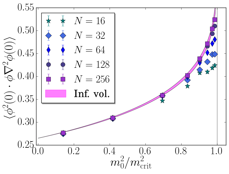
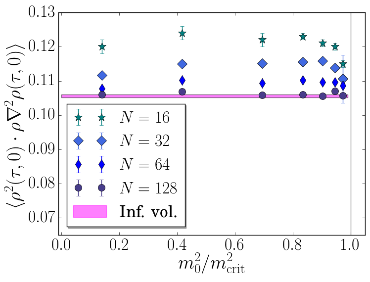
Figure 3: (Left) The matrix element $\left\langle\Omega|\phi^{2}(0)\cdot\phi(0)\nabla^{2}\phi(0)|\Omega\right\rangle$, as a function of the bare mass, expressed as a ratio of the critical mass, at fixed coupling. The magenta band shows a fit to a logarithmic function of $(1-m_{0}^{2}/m_{\mathrm{crit}}^{2})$ for the infinite volume results, obtained from a polynomial fit in $1/N$. (Right) The same matrix element, but at non-zero flow time. Here the magenta band is a fit to a constant. Including terms polynomial in the flow time does not change the final fit, within errors.

4 Conclusion

Power-divergent mixing complicates the continuum limit of lattice matrix elements for a wide range of calculations. The gradient flow provides a tool to remove power-divergent mixing from lattice calculations. Here I demonstrate this principle in the simple toy model of scalar field theory, with quartic interactions, in two dimensions. By keeping the flow time fixed in physical units in the continuum limit, power-divergent coefficients are rendered finite, at the expense of introducing a new physical scale into the system: the smearing radius.

One approach to dealing with this new scale is the smeared operator product expansion (sOPE), in which nonlocal operators are expanded in a basis of locally-smeared operators. The corresponding perturbative coefficients are then also functions of the smearing radius and, to a given order in perturbation theory and the flow time, the product of these perturbative coefficients with the matrix elements of smeared operators should be flow-time independent.

The sOPE also provides a natural framework for studying vacuum condensates and, in QCD, may provide sum-rule relations that relate vacuum matrix elements determined on the lattice to hadronic parameters. To extract meaningful physics, however, one must move beyond the toy model of two-dimensional scalar field theory, studied here, and implement the sOPE in QCD. This work is in progress.

- [1] C. Monahan and K. Orginos, Phys.Rev.D 91 (2015) 074513 [1501.05348]; C. Monahan and K. Orginos, \posPoS(LATTICE2014)330 (2014) [1410.3393]
- [2] M. Lüscher and P. Weisz, JHEP 1102 (2011) 051 [1101.5261]; M. Lüscher, JHEP 1304 (2013) 123 [1302.5246]; H. Makino and H. Suzuki, PTEP (2015) 033B08 [1410.7538]
- [3] C. Morningstar and M. Peardon, Phys.Rev.D 69 (2004) 054501 [hep-lat/0311018]
- [4] C. Dawson et al., Nucl.Phys.B 514 (1998) 313 [hep-lat/9707009]; W. Detmold and C.J.D. Lin, Phys.Rev.D 73 (2006) 014501 [hep-lat/0507007]; S. Caracciolo, A. Montanari and A. Pelissetto, JHEP 0009 (2000) 045 [hep-lat/0007044]
- [5] J.C. Collins, Renormalization, Cambridge University Press, Cambridge 1984
- [6] R. Narayanan and H. Neuberger, JHEP 0603 (2006) 064 [hep-th/0601210]
- [7] M. Dalla Brida, M. Garofalo and A.D. Kennedy, \posPoS(LATTICE 2015)309 (2015)
- [8] R. Loinaz and R.S. Willey, Phys.Rev.D 58 (1998) 076003 [hep-lat/9712008]; R. Toral and A. Chakrabarti, PRB 42 (1990) 2445
- [9] Z. Fodor et al., JHEP 1211 (2012) 007 [1208.1051]
- [10] U. Wolff, Phys.Rev.Lett. 62 (1989) 361
- [11] C. Morningstar, (2007) [hep-lat/0702020]; J. Goodman and A.D. Sokal, Phys.Rev.Lett. 56 (1986) 1015
- [12] U. Wolff, Comput.Phys.Commun. 156 (2004) 143 [hep-lat/0306017] [13] K. Binder, Z.Phys.B 43 (1981) 119; K. Binder, Phys.Rev.Lett. 47 (1981) 693