Nonlinear ion acoustic waves scattered by vortexes

Abstract

The Kadomtsev–Petviashvili (KP) hierarchy is the archetype of infinite-dimensional integrable systems, which describes nonlinear ion acoustic waves in two-dimensional space. This remarkably ordered system resides on a singular submanifold (leaf) embedded in a larger phase space of more general ion acoustic waves (low-frequency electrostatic perturbations). The KP hierarchy is characterized not only by small amplitudes but also by irrotational (zero-vorticity) velocity fields. In fact, the KP equation is derived by eliminating vorticity at every order of the reductive perturbation. Here we modify the scaling of the velocity field so as to introduce a vortex term. The newly derived system of equations consists of a generalized three-dimensional KP equation and a two-dimensional vortex equation. The former describes ‘scattering’ of vortex-free waves by ambient vortexes that are determined by the latter. We say that the vortexes are ‘ambient’ because they do not receive reciprocal reactions from the waves (i.e., the vortex equation is independent of the wave fields). This model describes a minimal departure from the integrable KP system. By the Painlevé test, we delineate how the vorticity term violates integrability, bringing about an essential three-dimensionality to the solutions. By numerical simulation, we show how the solitons are scattered by vortexes and become chaotic.

1 Introduction

The ion acoustic waves (IAWs) serve as a rich source of nonlinear phenomena. The combination of the nonlinearity (by fluid convection) and the dispersion (by the nonlocal electric interactions) enables IAWs to produce various structures ranging from order (such as solitons) to chaos (turbulences). At the simplest one-dimensional geometry, small-amplitude IAWs become solitons; Washimi and Taniuti [1] derived the Korteweg–de Vries (KdV) equation by the reductive perturbation method. The Kadomtsev–Petviashvili (KP) equation [2] is a two-dimensional generalization of the KdV equation, which was picked up by the ‘Kyoto School’ as the archetype of infinite-dimensional integrable systems [3, 4]. Kako and Rowlands [5] derived three types of two-dimensional generalizations of Washimi and Taniuti’s result, including the KP equation. Diverse directions of generalizations have been also studied; for example, variations of the KdV equation including finite ion temperature [6, 7], multi-ions [8], and dust plasma [9]; as well as variations of the KP equation including multi-ions [10], dust plasma [11], and multi-temperature [12, 13]. The modifications to include third-order nonlinear terms were proposed by considering trapped electrons [14, 15]. Effects of higher order terms in the reductive perturbation method have been also widely studied (see, e.g., Refs. [16, 17, 9] and references therein). The higher order perturbations are called clouds, and the solitons are called dressed solitons.

In this paper, we explore a new direction of generalization—we introduce a vorticity to the system, and delineate a fundamental change of dynamics brought about by the vortex. The KP hierarchy is characterized not only by small amplitudes but also by irrotational (zero-vorticity) velocity fields (see Section 2.2). We may view the ordered system of solitons as a singular submanifold (leaf) embedded in a larger phase space of finite-vorticity perturbations [18]. The departure from the zero-vorticity leaf will produce complexity and, finally, generate turbulence. The aim of this study is to probe into the ‘neighborhood’ of the KP hierarchy and elucidate how chaos starts to develop.

We organize this paper as follows. In Section 2, we show that the KP equation is derived by eliminating vorticity at every order of the reductive perturbation. We also show that the reductive perturbation succeeds only if the entropy is homogeneous; hence the baroclinic effect, a creation mechanism of vorticity, must be absent (A). In Section 3, we introduce a new ordering of velocity field in order to formulate a finite-vorticity system. The new system is composed of a generalized three-dimensional KP equation and a two-dimensional vorticity equation. The former describes ‘scattering’ of vortex-free waves by ambient vortexes that are determined by the latter. We say that the vortexes are ‘ambient’ because they do not receive reciprocal reactions from the waves. In Section 4, we invoke the Painlevé test to study whether the new system is integrable or not. The result is negative. By this analysis, we elucidate that the scattering by the vorticity introduces an essential three-dimensionality in the wave fields, by which the integrability condition (in the sense of the Painlevé test) is broken. In Section 5, we perform numerical simulations to visualize how chaos occurs. Section 6 concludes our investigations.

2 Reductive perturbation method for Kadomtsev–Petviashvili equation and vorticity

2.1 Kadomtsev–Petviashvili equation

We start by remembering the derivation of the KP equation by the reductive perturbation method [1, 5, 2]. The basic equations for nonlinear IAWs are expressed as

$$\frac{\partial n}{\partial t}+\nabla\cdot(n\boldsymbol{u})=0,$$ (1)

$$\frac{\partial\boldsymbol{u}}{\partial t}+(\boldsymbol{u}\cdot\nabla)\boldsymbol{u}=\nabla\phi,$$ (2)

$$-\Delta\phi=n-\mathrm{e}^{\phi},$$ (3)

where $n$ is the ion number density, $\boldsymbol{u}=(u,v,w)^{\top}$ is the ion velocity, $\phi$ is the electrostatic potential, and $\Delta$ is the Laplacian. We consider cold ions and adiabatic electrons with a constant temperature $T_{\mathrm{e}}$. The variables are normalized as followings: the density $n$ by a representative density $n_{0}$, the velocity $\boldsymbol{u}$ by the ion sound speed $c_{\mathrm{s}}=\sqrt{T_{\mathrm{e}}/m_{\mathrm{i}}}$ (where $m_{\mathrm{i}}$ is the ion mass), the electrostatic potential $\phi$ by the characteristic potential $T_{\mathrm{e}}/e$, the coordinate variable $\boldsymbol{x}$ by the Debye length $\sqrt{\varepsilon_{0}T_{\mathrm{e}}/n_{0}e^{2}}$, and the time variable $t$ by the ion plasma frequency $\sqrt{n_{0}e^{2}/\varepsilon_{0}m_{\mathrm{i}}}$.

We consider IAWs propagating in two-dimensional space $(x,y)$. The extension to three-dimensional space $(x,y,z)$ will be discussed later. We assume that waves propagate primarily in the direction of $x$, and introduce a set of stretched variables

$$\tilde{x}=\epsilon(x-t),\qquad\tilde{y}=\epsilon^{2}y,\qquad\tilde{t}=\epsilon^{3}t,$$ (4)

with a small parameter $\epsilon$. The dependent variables $n$, $\phi$, $u$, and $v$ are expanded as

$$\left\{\begin{aligned} n&=1+\epsilon^{2}n_{1}+\epsilon^{4}n_{2}+\cdots,\\ \phi&=0+\epsilon^{2}\phi_{1}+\epsilon^{4}\phi_{2}+\cdots,\\ u&=0+\epsilon^{2}u_{1}+\epsilon^{4}u_{2}+\cdots,\\ v&=0+\epsilon^{3}v_{1}+\epsilon^{5}v_{2}+\cdots.\end{aligned}\right.$$ (5)

From the terms of orders $\epsilon^{2}$ and $\epsilon^{3}$, we obtain $n_{1}=\phi_{1}$ and $\partial n_{1}/\partial\tilde{x}=\partial u_{1}/\partial\tilde{x}=\partial\phi_{1}/\partial\tilde{x}$. Assuming the boundary conditions $n_{1},\phi_{1},u_{1}\to 0$ $(x\to\pm\infty)$, we put

$$n_{1}=u_{1}=\phi_{1}.$$ (6)

From the terms of order $\epsilon^{4}$, we obtain

$$\frac{\partial v_{1}}{\partial\tilde{x}}=\frac{\partial\phi_{1}}{\partial\tilde{y}}$$ (7)

and $n_{2}=\phi_{2}+\phi_{1}^{2}/2-\partial^{2}\phi_{1}/\partial{\tilde{x}}^{2}$. From the terms of order $\epsilon^{5}$, we obtain the two-dimensional KP equation:

$$\frac{\partial}{\partial\tilde{x}}\left(\frac{\partial\phi_{1}}{\partial\tilde{t}}+\phi_{1}\frac{\partial\phi_{1}}{\partial\tilde{x}}+\frac{1}{2}\frac{\partial^{3}\phi_{1}}{\partial\tilde{x}^{3}}\right)+\frac{1}{2}\frac{\partial^{2}\phi_{1}}{\partial\tilde{y}^{2}}=0.$$ (8)

In three-dimensional space $(x,y,z)$, we introduce a stretched variable $\tilde{z}$ and expand the velocity $w$ as

$$\tilde{z}=\epsilon^{2}z,\qquad w=0+\epsilon^{3}w_{1}+\epsilon^{5}w_{2}+\cdots.$$ (9)

From the terms of order $\epsilon^{4}$, we obtain the relation

$$\frac{\partial w_{1}}{\partial\tilde{x}}=\frac{\partial\phi_{1}}{\partial\tilde{z}},$$ (10)

which parallels equation (7). The terms of order $\epsilon^{5}$ lead to the three-dimensional KP equation

$$\frac{\partial}{\partial\tilde{x}}\left(\frac{\partial\phi_{1}}{\partial\tilde{t}}+\phi_{1}\frac{\partial\phi_{1}}{\partial\tilde{x}}+\frac{1}{2}\frac{\partial^{3}\phi_{1}}{\partial\tilde{x}^{3}}\right)+\frac{1}{2}\Delta_{\perp}\phi_{1}=0,$$ (11)

where $\Delta_{\perp}=(\partial/\partial{\tilde{y}})^{2}+(\partial/\partial{\tilde{z}})^{2}$.

2.2 Vorticity of Kadomtsev–Petviashvili equation

Strikingly absent in the KP system is the vorticity. The $z$-component of the vorticity $\omega_{z}=\partial v/\partial x-\partial u/\partial y$ is expanded as

$$\omega_{z}=\epsilon^{4}\left(\frac{\partial v_{1}}{\partial\tilde{x}}-\frac{\partial u_{1}}{\partial\tilde{y}}\right)+\epsilon^{6}\left(\frac{\partial v_{2}}{\partial\tilde{x}}-\frac{\partial u_{2}}{\partial\tilde{y}}\right)+\cdots.$$ (12)

The leading-order term turns out to be zero from equations (6) and (7). The same ordering applies to the $y$-component of the vorticity $\omega_{y}=\partial u/\partial z-\partial w/\partial x$; hence the leading-order vorticity vanishes by the demand of equations (6) and (10). The $x$-component of the vorticity $\omega_{x}=\partial w/\partial y-\partial v/\partial z$ is expanded as

$$\omega_{x}=\epsilon^{5}\left(\frac{\partial w_{1}}{\partial\tilde{y}}-\frac{\partial v_{1}}{\partial\tilde{z}}\right)+\epsilon^{7}\left(\frac{\partial w_{2}}{\partial\tilde{y}}-\frac{\partial v_{2}}{\partial\tilde{z}}\right)+\cdots.$$ (13)

The ordering is slightly different from those of $\omega_{y}$ and $\omega_{z}$. However, the leading-order term is forced to vanish by equations (6), (7), (10), and the boundary condition $\partial w_{1}/\partial\tilde{y}-\partial v_{1}/\partial\tilde{z}\to 0$ $(x\to\pm\infty)$. Thus, the KP system is vortex-free.

In A, we discuss a finite-temperature system, in which an inhomogeneous entropy yields a baroclinic effect, a mechanism creating vorticity. Then, the aforementioned ordering fails to formulate a reductive perturbation, implying that the KP system is fundamentally incapable to host a vorticity.

2.3 Vorticity of general order

The absence of vorticity is not only at the order of KP equation, but also at all orders of perturbations. Let us examine higher order equations. The second-order equation is linear with respect to the second-order variables, and includes an inhomogeneous term depending on $\phi_{1}$ [17, 16, 9]. The higher order perturbations are called clouds surrounding the core, i.e., the first-order perturbation; a soliton with clouds is called a dressed soliton. As proved in the previous section, the core is vortex-free. Moreover, we find that all higher order clouds are vortex-free.

The vorticity equation is derived by taking the curl $\nabla\times{}$ of the equation of motion (2):

$$\frac{\partial\boldsymbol{\omega}}{\partial t}=\nabla\times(\boldsymbol{u}\times\boldsymbol{\omega}).$$ (14)

After the Galilean boost in the $x$-direction (see equation (4)), equation (14) reads as

$$\frac{\partial\boldsymbol{\omega}}{\partial t}-\frac{\partial\boldsymbol{\omega}}{\partial x}=\nabla\times(\boldsymbol{u}\times\boldsymbol{\omega}).$$ (15)

Inserting the expressions (4) and (5), and using equations (9), (12), and (13), let us see the orders of each term in equation (15); in the $x$-component

$$\frac{\partial\omega_{x}}{\partial t}-\frac{\partial\omega_{x}}{\partial x}=\frac{\partial}{\partial y}(u\omega_{y}-v\omega_{x})-\frac{\partial}{\partial z}(w\omega_{x}-u\omega_{z}),$$ (16)

the order of the second term on the left-hand-side is $\epsilon^{6}$, while all other terms are of order $\epsilon^{8}$. Thus, the lowest order vorticity $\omega_{x1}$ must satisfy $\partial\omega_{x1}/\partial x=0$. By the boundary condition $\omega_{x1}\to 0$ $(x\to\pm\infty)$, therefore, we obtain $\omega_{x1}=0$. In the $y$- and $z$-components of equation (15), the orders of all terms decrease by $\epsilon^{1}$; hence we obtain $\omega_{y1}=\omega_{z1}=0$ under the boundary conditions $\omega_{y1},\omega_{z1}\to 0$ $(x\to\pm\infty)$.

Eliminating $\boldsymbol{\omega}_{1}$, equation (15) reads as the equation for $\boldsymbol{\omega}_{2}$ (the second-order part of $\boldsymbol{\omega}$). By the same argument of ordering, we obtain $\boldsymbol{\omega}_{2}=0$, and equation (15) dominates the next order. Continuing the induction, we conclude that $\boldsymbol{\omega}_{j}=0$ for all order $j$.

3 Generalized system with finite vorticity

We can formulate a generalized system with a finite vorticity by introducing a velocity $\boldsymbol{v}_{0}=(0,v_{0},w_{0})^{\top}$ of order $\epsilon^{1}$ in the $y$- and $z$-directions:

$$\left\{\begin{aligned} v&=\epsilon v_{0}+\epsilon^{3}v_{1}+\epsilon^{5}v_{2}+\cdots,\\ w&=\epsilon w_{0}+\epsilon^{3}w_{1}+\epsilon^{5}w_{2}+\cdots.\end{aligned}\right.$$ (17)

We assume that the additional velocity is homogeneous in the $x$-direction ($\partial\boldsymbol{v}_{0}/\partial x=\boldsymbol{0}$) and incompressible ($\nabla\cdot\boldsymbol{v}_{0}=0$). By the two-dimensionality and incompressibility, we may write $\boldsymbol{v}_{0}$ in a Clebsch form [19]

$$\boldsymbol{v}_{0}=\nabla_{\perp}\psi(\tilde{y},\tilde{z})\times\boldsymbol{e}_{x},$$ (18)

where $\boldsymbol{e}_{x}$ is the unit vector in the $x$-direction, $\psi$ is the stream function, and $\nabla_{\perp}=(0,\partial/\partial\tilde{y},\partial/\partial\tilde{z})$.

From the lowest order terms, we obtain the conventional two-dimensional Euler vorticity equation

$$\frac{\partial}{\partial\tilde{t}}\Delta_{\perp}\psi+[\Delta\psi,\psi]=0,$$ (19)

where $\Delta_{\perp}\psi$ denotes the vorticity and $[f,g]=\boldsymbol{e}_{x}\cdot(\nabla_{\perp}f\times\nabla_{\perp}g)=(\partial f/\partial\tilde{y})(\partial g/\partial\tilde{z})-(\partial f/\partial\tilde{z})(\partial g/\partial\tilde{y})$. From the terms of order $\epsilon^{5}$, we obtain a three-dimensional wave equation:

$$\frac{\partial}{\partial\tilde{x}}\left(\frac{\partial\phi_{1}}{\partial\tilde{t}}+\phi_{1}\frac{\partial\phi_{1}}{\partial\tilde{x}}+\frac{1}{2}\frac{\partial^{3}\phi_{1}}{\partial\tilde{x}^{3}}+[\phi_{1},\psi]\right)+\frac{1}{2}\Delta_{\perp}\phi_{1}=0.$$ (20)

For the convenience, we call the system of equations (19) and (20) Kadomtsev–Petviashvili–Yoshida (KPY) equations and compare it with the KP equation. In what follows, the subscript ₁ and tilde $\tilde{\hphantom{x}}$ will be omitted for simplicity.

The vortex field $\psi$ ($\Delta_{\perp}\psi$ is the vorticity) affects the wave field $\phi$ through equation (20) while it does not receive any reciprocal reaction from $\phi$ (notice that the vortex equation (19) is independent of $\phi$). This is because the order of $\psi$ is lower than that of $\phi$. We may treat $\psi$ as an ‘ambient’ field for $\phi$.

In the rest of paper, we assume that the vortex field $\psi$ is stationary. For example, $\psi=a\sin(ky)-a\cos(kz)$ is a stationary solution of the Euler equation (19), which satisfies $\Delta_{\perp}\psi\propto\psi$. Then, only (20), to be called the KPY equation, will be the target of analysis.

4 Painlevé analysis

Here we put the KPY equation to the Painlevé test. Let us begin by reviewing the method briefly. According to Weiss, Tabor, and Carnevale (WTC) [20], a nonlinear partial differential equation (PDE) is said to have the Painlevé property when the solutions are represented in terms of a Laurent series in a neighborhood of a movable singularity manifold (to be identified as a set of points satisfying $\varphi(x,y,z,t)=0$); assuming that the solution $\phi(x,y,z,t)$ of PDE can be written, in the neighborhood of the singularity manifold, as

$$\phi(x,y,z,t)=\chi^{-q}\sum_{j=0}^{\infty}\phi_{j}(x,y,z,t)\chi^{j}$$ (21)

with analytic functions $\phi_{j}$ and an expansion function $\chi$ which vanishes as $\varphi\rightarrow 0$, the Painlevé property is tested by verifying that $q$ is a positive integer and that all $\phi_{j}$’s can be determined consistently. There are various choices of the expansion function $\chi$. The most natural one is $\chi=\varphi$, which is used by WTC [20]. However, this choice makes $\phi_{j}$ complicated. Conte [21] has shown that the best choice for reducing the calculation without any constraints on $\varphi$ is

$$\chi=\left(\frac{\varphi_{x}}{\varphi}-\frac{\varphi_{xx}}{2\varphi_{x}}\right)^{-1},$$ (22)

where subscripts denote derivatives, e.g., $\varphi_{x}=\partial\varphi/\partial x$. (A constraint $\varphi_{x}=0$ is required, however, this is also necessary for WTC and other choices.) For details of the Painlevé analysis for PDEs, see, e.g., Ref. [22].

The Painlevé property is considered to be equivalent to the integrability of a PDE, and many integrable equations (e.g., the Burgers equation, the KdV equation, and the two-dimensional KP equation) pass the Painlevé test [20]. However, the three-dimensional KP equation does not pass the test [23, 24, 25], and it is not integrable (see, e.g., Ref. [26] for another explanation of its non-integrability). Since the additional vortex field is perpendicular to the primal direction of propagation, it brings about an essential three-dimensionality. Thus, it is expected that the KPY equation (20) is not integrable.

Now we execute the Painlevé test for the KPY equation (20) with Conte’s choice (22) and show that the KPY equation passes the Painlevé test only under some special conditions. In order to elucidate when the equation is integrable or not, we use a generalized form

$$\phi_{xt}+(\phi\phi_{x})_{x}+\alpha\phi_{4x}+\beta\phi_{yy}+\gamma\phi_{zz}+a(y,z)\phi_{xy}+b(y,z)\phi_{xz}=0,$$ (23)

where $\alpha,\beta,\gamma$ are constants with $\alpha\neq 0$ and $a,b$ are functions of $y,z$. In the original form (20), coefficients are chosen as $\alpha=1$, $\beta=\gamma=1/2$, $a(y,z)=\partial\psi/\partial z$, and $b(y,z)=-\partial\psi/\partial y$.

The leading-order analysis (substituting $\phi=\phi_{0}\chi^{-q}$ and comparing leading-order terms) determines the values of $q$ and $\phi_{0}$ as $q=2$ and $\phi_{0}=-12\alpha$. From general order terms, we obtain recursion relations

$$(j+1)(j-4)(j-5)(j-6)\alpha\phi_{j}=F_{j}(\phi_{0},\ldots,\phi_{j-1})$$ (24)

for $j=1,2,\ldots{}$, where $F_{j}$’s are complicated functions of $\phi_{0},\ldots,\phi_{j-1}$, $\varphi$, and their derivatives. $\phi_{1}$, $\phi_{2}$, and $\phi_{3}$ are determined by equation (24), and $F_{4}=F_{5}=F_{6}=0$ is required for consistency (called a resonance condition). When the condition puts no constraint on $\varphi$, we can determine all $\phi_{j}$’s cotnsistently with arbitrary functions $\phi_{4}$, $\phi_{5}$, and $\phi_{6}$. The two-dimensional KP equation (8) satisfies the resonance condition, however, the three-dimensional KP equation (11) and KPY equation (20) do not satisfy that. In the latter case, we find $F_{4}=F_{5}=0$ and $F_{6}\neq 0$. For the KPY equation (23), $F_{6}$ is expressed as

$$F_{6} =\beta\gamma E_{1}(\varphi)+\beta E_{2}(a_{y},a_{yy},b_{y},b_{yy};\varphi)+\gamma E_{3}(a_{z},a_{zz},b_{z},b_{zz};\varphi),$$ (25)

$$E_{1} =\frac{4}{\varphi_{x}^{4}}\bigl{[}\varphi_{x}^{2}(\varphi_{yy}\varphi_{yz}-\varphi_{yz}^{2})+2\varphi_{x}\varphi_{y}(\varphi_{xz}\varphi_{yz}-\varphi_{xy}\varphi_{zz})+\circlearrowleft_{x,y,z}\bigr{]},$$ (26)

$$E_{2} =\frac{1}{\varphi_{x}^{3}}\bigl{[}-a_{yy}\varphi_{x}^{2}\varphi_{y}-b_{yy}\varphi_{x}^{2}\varphi_{z}-2a_{y}\varphi_{x}^{2}\varphi_{yy}-2b_{y}\varphi_{x}^{2}\varphi_{yz}$$

$$\hskip 30.35326pt+2(2a_{y}+b_{y})\varphi_{x}\varphi_{z}\varphi_{xy}+2b_{y}\varphi_{x}\varphi_{y}\varphi_{xz}-2b_{y}\varphi_{xx}\varphi_{y}\varphi_{z}-2a_{y}\varphi_{xx}\varphi_{y}^{2}\bigr{]},$$ (27)

$$E_{3} =\frac{1}{\varphi_{x}^{3}}\bigl{[}-a_{zz}\varphi_{x}^{2}\varphi_{y}-b_{zz}\varphi_{x}^{2}\varphi_{z}-2a_{z}\varphi_{x}^{2}\varphi_{yz}-2b_{z}\varphi_{x}^{2}\varphi_{zz}$$

$$\hskip 30.35326pt+2(a_{z}+2b_{z})\varphi_{x}\varphi_{y}\varphi_{xz}+2a_{z}\varphi_{x}\varphi_{z}\varphi_{xy}-2a_{z}\varphi_{xx}\varphi_{y}\varphi_{z}-2b_{z}\varphi_{xx}\varphi_{z}^{2}\bigr{]}.$$ (28)

where $\circlearrowleft_{x,y,z}$ denotes the summation over cyclic permutation of $x,y,z$. $E_{1}$ is $F_{6}$ of the three-dimensional KP equation [23].

The resonance condition $F_{6}=0$ is satisfied only in the following special cases: (i) $\beta=\gamma=0$; (ii) $\gamma=0$, $a_{y}=b_{y}=0$; (iii) $\beta=0$, $a_{z}=b_{z}=0$. In the case (i), the KPY equation (23) is reduced to the one-dimensional $(x)$ KdV equation with advection terms in the independent directions ($y,z$). In the case (ii), the KPY equation is reduced to the two-dimensional $(x,y)$ KP equation with Galilean boosting (whose speed is homogeneous in $x$- and $y$-directions). The case (iii) is same as the case (ii), with $y$ and $z$ exchanged. The cases (ii) and (iii) are consistent with integrable conditions of generalized variable-coefficient two-dimensional KP equations, see, e.g., Ref. [27].

From the above result, we find that the KPY equation is integrable only if it can be reduced to a lower dimensional integrable system (the one-dimensional KdV equation or the two-dimensional KP equation). In the next section, we demonstrate chaotic behaviors of IAW by numerical solutions of the KPY equation.

5 Numerical analysis

5.1 Settings of numerical simulation

We perform numerical simulation by the following setting. We consider a domain $(x,y,z)\in[0,20]\times[-5,5]\times[-5,5]$ with the periodic boundary condition. The KPY equation (20) is solved in the following splitting form:

$$\frac{\partial\phi}{\partial t} =\mathcal{L}\phi+\mathcal{N}(\phi),$$ (29)

$$\mathcal{L}\phi =-\frac{1}{2}\frac{\partial^{3}\phi}{\partial x^{3}}-\frac{1}{2}\partial_{x}^{-1}\Delta_{\perp}\phi,$$ (30)

$$\mathcal{N}(\phi) =-\frac{1}{2}\frac{\partial}{\partial x}(\phi^{2})-[\phi,\psi],$$ (31)

with the second-order Strang splitting method [28]

$$\phi_{n+1}=\exp\left(\frac{h}{2}\mathcal{L}\right)\exp(h\mathcal{N})\exp\left(\frac{h}{2}\mathcal{L}\right)\phi_{n},$$ (32)

where $h$ is the time step size. Each factor on the right-hand side of equation (32) must be approximated by a second or higher order scheme. Here, the linear evolution $\exp(h\mathcal{L})$ is solved implicitly with the Fourier transformation, while the nonlinear evolution $\exp(h\mathcal{N})$ is approximated by the second-order Runge–Kutta method with finite-difference approximations. The anti-derivative $\partial_{x}^{-1}$ in the linear operator $\mathcal{L}$ can be calculated by the Fourier multiplier $-\mathrm{i}/k_{x}$. In order to regularize the singularity at $k_{x}=0$, this multiplier is modified as $-\mathrm{i}/(k_{x}+\mathrm{i}\delta)$, with a small real number $\delta$ (we use the machine epsilon of double precision floating point number $2^{-52}\sim 2.2\times 10^{-16}$) [29, 30, 31].

We give an initial condition by modifying the single soliton solution of the two-dimensional KP equation:

$$\phi_{0}(x,y,z)=3A\operatorname{sech}^{2}\left[\sqrt{\frac{A}{2}}(x-By-C)\right],$$ (33)

where $A$, $B$, and $C$ are arbitrary constants (we choose $A=1$, $B=2$, and $C=10$). To put the waves in the periodic domain, $x$ and $y$ are, respectively, modulo 20 and 10 (box sizes). Furthermore, $\phi$ must satisfy

$$\int\Delta_{\perp}\phi\,\mathrm{d}x=0,$$ (34)

which is derived by integrating the KPY equation (20) in the $x$-direction. By subtracting the Fourier components with $k_{x}=0$ ($k_{x}$ is the wave number in the $x$ direction), excepting the $k_{x}=k_{y}=k_{z}=0$ component, from $\phi_{0}(x,y,z)$, we obtain the hoped-for initial condition. The KP equation (i.e., $\psi=0$), starting from this initial condition, propagates with conserving the wave shape.

As described at the end of Section 3, we assume that $\psi$ is stationary. We use

$$\psi(y,z)=a\sin\left(\frac{2\pi\kappa y}{L}\right)-a\cos\left(\frac{2\pi\kappa z}{L}\right),$$ (35)

where $L$ is the length of the domain in the $y$- and $z$-directions ($L=10$). $a$ and $\kappa$ denote the intensity and the wavenumber of the vortex field. We change their values and observe how line-solitons are ‘scattered’ by the vortex.

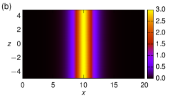
Figure 1: Cross-sections of $\phi$ at $t=0$ (a line-soliton with the periodic boundary condition, homogeneous in the $z$-direction). (a) $(z=0)$-cross-section, (b) $(y=0)$-cross-section.

5.2 Numerical results

When $a=0$ (vortex-free), a line-soliton propagates without changing its shape. Figures 2 and 3 show $y$- and $z$-cross-sections of $\phi$ with $a=0.06$ and $\kappa=2$. In Fig. 2, we observe deformations in the $y$-cross-sections: (i) to the right side (Fig. 2a); (ii) to both sides (Fig. 2b); (iii) to the left side (Fig. 2c); (iv) after (i)–(iii), $\phi$ returns to the initial shape, homogeneous in the $z$-direction (Fig. 2d). We find that the deformations (i)–(iv) are repeated periodically. In the $z$-cross-section, compared to the $y$-cross-section, noticeable deformations are not found (Fig. 3). From these results, we can say that line-solitons (homogeneous in the $z$-direction) are ‘stable’ against weak vortexes.

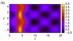
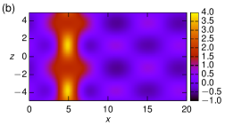
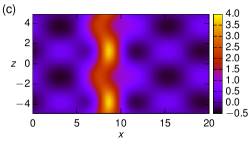
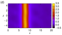
Figure 2: $(y=0)$-cross-sections of $\phi$ with $a=0.06$ and $\kappa=2$ at different times. (a) $t=25$, (b) $t=32$, (c) $t=40$: the direction of deformation is changed with time. (d) $t=60$: after the deformation, $\phi$ becomes homogeneous in $z$-direction, as in the initial state (Fig. 1b).

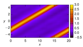
Figure 3: $(z=0)$-cross-section of $\phi$ with $a=0.06$ and $\kappa=2$ at $t=32$.

Figures 4 and 5 show $y$- and $z$-cross-sections of $\phi$ with a larger value of $a$ ($a=0.30$). In the $y$-cross-section (Fig. 4), We observe divided structures without returning to the initial shape. Furthermore, differently from the result of $a=0.06$, deformations in the $z$-cross-section is also observed (Fig. 5). When $a$ is further large, $\phi$ breaks up into small structures and spreads, as found in Fig. 6. These results show scatterings of line-solitons due to the ambient vortex fields, and they can be regarded as effects of the non-integrability.

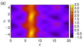
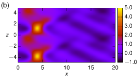
Figure 4: $(y=0)$-cross-sections of $\phi$ with $a=0.30$ and $\kappa=2$ at different times: (a) $t=20$, (b) $t=40$.

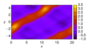
Figure 5: $(z=0)$-cross-section of $\phi$ with $a=0.30$ and $\kappa=2$ at $t=40$.

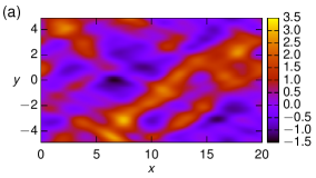
Figure 6: Cross-sections of $\phi$ at $t=40$ with $a=1.0$ and $\kappa=2$: (a) ($z=0$)-cross-section, (b) ($y=0$)-cross-section.

To evaluate the above observations quantitatively, we calculate the average wavenumber

$$\langle k_{j}\rangle=\frac{\sum_{\boldsymbol{k}}k_{j}|\hat{\phi}_{\boldsymbol{k}}|^{2}}{\sum_{\boldsymbol{k}}|\hat{\phi}_{\boldsymbol{k}}|^{2}}\quad(j=x,y,z),$$ (36)

where $\hat{\phi}_{\boldsymbol{k}}$’s are Fourier coefficients of $\phi$. Figure 7 shows the evolution of the average wavenumber $\langle k_{y}\rangle$ with $a=0.02$, $0.04$, $0.06$, and $0.08$ ($\kappa=2$ is fixed). One can find that the evolution looks like periodic and the period becomes short when $a$ becomes large. Figure 8 shows the evolution of $\langle k_{y}\rangle$ with $a=0.08$, $0.09$, and $0.10$. A transition from the periodic behavior ($a=0.08$) to the increasing behavior ($a=0.09,0.10$) is found. As shown in Fig. 9, the average wavenumber has a large value when $a$ is further large. In this stage, periodic evolutions are not observed. One also finds that the value of the average wavenumber is not clearly different between in the case of $a=0.8$ and in that of $a=1.0$. When $\kappa$ has a large value, the average wavenumber is found to grow larger (Fig. 10). Thus, we can say that scattering scales of line-solitons depend on the intensity and the spatial scales of the ambient vortex fields.

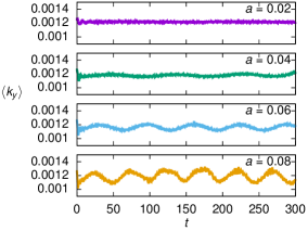
Figure 7: Evolution of average wavenumber $\langle k_{y}\rangle$ with $a=0.02,0.04,0.06,0.08$. $\kappa=2$ is fixed.

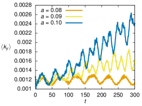
Figure 8: Evolution of average wavenumber $\langle k_{y}\rangle$ with $a=0.08,0.09,0.10$. $\kappa=2$ is fixed.

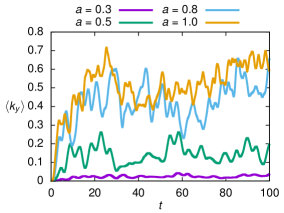
Figure 9: Evolution of average wavenumber $\langle k_{y}\rangle$ with $a=0.3,0.5,0.8,1.0$. $\kappa=2$ is fixed.

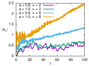
Figure 10: Evolution of average wavenumber $\langle k_{y}\rangle$ with $(a,\kappa)=(0.8,2)$, $(1.0,2)$, $(0.8,8)$, $(1.0,8)$.

6 Conclusion

The challenge of imparting vorticity to IAW was overcome by modifying the ordering of velocity field. The newly formulated nonlinear system describes the scattering of IAWs propagating in the ambient vortex field. The Painlevé test on the new system elucidates that the vorticity introduces essential three-dimensionality to the wave, by which the integrability of the two-dimensional KP system is destroyed. When the ambient vortex is weak, a two-dimensional line-soliton is deformed periodically but keep the solitary-wave structure. This result indicates that a two-dimensional line-soliton is stable near the zero-vorticity state, even though the evolution equation is non-integrable. The non-integrability (chaotic property) is found when the ambient vortex is strong; line-solitons are broken into small scattered waves.

We end this paper with additional comments. As we have shown in Section 2.3, the absence of vorticity is a strong imprint made by the ordering that characterizes the KP system. This constraint is ubiquitous among the families including a finite-temperature model (see A), trapped electron model, and multi-component models (see the references cited in Introduction).

The new ordering of the velocity field enables us to study the neighborhood of the integrable KP hierarchy. At the lowest order, i.e., the KPY system, however, the range of dynamics is still rather narrow. In fact, the helicity $\int\boldsymbol{u}\cdot\boldsymbol{\omega}\,\mathrm{d}^{3}x$ (the invariant characterizing the foliated phase space of general IAW [18]) is zero for the KPY system; by equation (34), we find

$$\int\phi\Delta_{\perp}\psi\,\mathrm{d}^{3}x=\int\psi\left(\int\Delta_{\perp}\phi\,\mathrm{d}x\right)\mathrm{d}y\,\mathrm{d}z=0.$$ (37)

The generalized enstrophy $\int g(\Delta_{\perp}\psi)\,\mathrm{d}^{2}x$ is also conserved ($g$ is an arbitrary function). The constancy of this integral is not only due to the geometrical constraint (two-dimensionality) of $\psi$ but also because of the absence of the reciprocal reaction from the wave field $\phi$. For a full development of turbulence, the enstrophy must be freed to increase, which is possible beyond the range of the present ordering.

Appendix A Finite ion temperature effect

In the vorticity equation (15), the boost term $\partial\boldsymbol{\omega}/\partial x$ causes unbalance of ordering and forces the vorticity to vanish, when we invoke the standard expansion (5) (this ordering is tailor-made to match $n(\nabla\cdot\boldsymbol{v})$ and $\nabla\phi$ with the boost terms in the continuity equation and the equation of motion).

In this appendix, we examine the effect of finite ion temperature $T_{\mathrm{i}}$. This introduces a non-potential force $-n^{-1}\nabla p$ to the equation of motion (2) and a source term $\nabla T_{\mathrm{i}}\times\nabla s$ to the vorticity equation (14), where $p$ is the ion pressure and $s$ is the ion entropy. This production mechanism of vorticity is called the baroclinic effect [32, 33]. We show that the baroclinic effect must be absent for the success of the reductive perturbation method.

We apply the reductive perturbation method for the KP equation (Section 2.1). We assume that the ion pressure is governed by the adiabatic equation

$$\frac{\partial p}{\partial t}+\boldsymbol{u}\cdot\nabla p+\Gamma p(\nabla\cdot\boldsymbol{u})=0,$$ (38)

where $\Gamma$ is the heat ratio. The pressure is normalized by the representative pressure $n_{0}T_{\mathrm{e}}$. We expand $p$ as $p=\sigma+\epsilon^{2}p_{1}+\epsilon^{4}p_{2}+\cdots{}$, where $\sigma=T_{\mathrm{i}0}/T_{\mathrm{e}}$ is the normalized representative temperature. It should be noted that the speed of Galilean boost must be modified from $1$ to $\lambda=\sqrt{1+\Gamma\sigma}$ (normalized with $c_{\mathrm{s}}=\sqrt{T_{\mathrm{e}}/m_{\mathrm{i}}}$) [7]. The relations (6), (7), and (10) are modified as

$$\left\{\begin{aligned} \lambda n_{1}&=\lambda\phi_{1}=u_{1}=\frac{\phi_{1}+p_{1}}{\lambda},\\ \frac{\partial v_{1}}{\partial\tilde{x}}&=\frac{1}{\lambda}\frac{\partial}{\partial\tilde{y}}(\phi_{1}+p_{1}),\\ \frac{\partial w_{1}}{\partial\tilde{x}}&=\frac{1}{\lambda}\frac{\partial}{\partial\tilde{z}}(\phi_{1}+p_{1}),\end{aligned}\right.$$ (39)

and we obtain the KP equation

$$\frac{\partial}{\partial\tilde{x}}\left[\frac{\partial\phi_{1}}{\partial\tilde{t}}+\left(1+\frac{\Gamma+1}{2}\Gamma\sigma\right)\phi_{1}\frac{\partial\phi_{1}}{\partial\tilde{x}}+\frac{1}{2\lambda}\frac{\partial^{3}\phi_{1}}{\partial\tilde{x}^{3}}\right]+\frac{\lambda}{2}\Delta_{\perp}\phi_{1}=0,$$ (40)

which reduces to equation (11) in the limit $T_{\mathrm{i}}=0$ ($\sigma=0$, $\lambda=1$).

From equation (39), we find that the lowest order vorticity is zero: $\omega_{x1}=\omega_{y1}=\omega_{z1}=0$, same as the case of cold ions ($T_{\mathrm{i}}=0$). Furthermore, we show that entropy must be homogeneous and thus baroclinic term must vanishes for the success of the reductive perturbation method. We use the same procedure of Section 2.3. Let us consider the adiabatic evolution equation for entropy

$$\frac{\partial s}{\partial t}+\boldsymbol{u}\cdot\nabla s=0,$$ (41)

which is equivalent to the pressure equation (38). The Galilean boost in the $x$-direction modifies equation (41) as

$$\frac{\partial s}{\partial t}-\lambda\frac{\partial s}{\partial x}+\boldsymbol{u}\cdot\nabla s=0.$$ (42)

Now we evaluate the orders of operators $\partial/\partial t$, $\lambda\partial/\partial x$, and $\boldsymbol{u}\cdot\nabla=u\partial/\partial x+v\partial/\partial y+w\partial/\partial z$ with equations (4), (5), and (9). The order of the second operator is $\epsilon^{1}$, and the lowest order of others is $\epsilon^{3}$. Thus, the leading order of entropy $s_{0}$ must satisfy $\partial s_{0}/\partial x=0$. This results in $s_{0}=c$ (constant) under the boundary condition $s_{0}\to c$ $(x\to\pm\infty)$, which is a natural choice because $s_{0}$ is not a perturbation part. Eliminating $s_{0}$, equation (42) reads as the equation for $s_{1}$. The same discussion requires $s_{1}$ to satisfy $\partial s_{1}/\partial x=0$. Since $s_{1}$ is a perturbation part, it is natural to use the boundary condition $s_{1}\to 0$ $(x\to\infty)$. These relations lead to $s_{1}=0$. Repeating this procedure, we find that entropy must be homogeneous: $s=s_{0}=c$.

We note that baroclinic effect vanishes even in our finite-vorticity system (Section 3). This is because the above discussion is valid even if we introduce the additional velocity $\boldsymbol{v}_{0}$ as equation (17). Finite ion temperature modifies the KPY equation (20) as

$$\frac{\partial}{\partial\tilde{x}}\left[\frac{\partial\phi_{1}}{\partial\tilde{t}}+\left(1+\frac{\Gamma+1}{2}\Gamma\sigma\right)\phi_{1}\frac{\partial\phi_{1}}{\partial\tilde{x}}+\frac{1}{2\lambda}\frac{\partial^{3}\phi_{1}}{\partial\tilde{x}^{3}}+[\phi_{1},\psi]\right]+\frac{\lambda}{2}\Delta_{\perp}\phi_{1}=0,$$ (43)

without changing the Euler vorticity equation (19).

References

- Washimi and Taniuti [1966] Washimi H, Taniuti T. Propagation of ion-acoustic solitary waves of small amplitude. Phys Rev Lett 1966;17(19):996–8. doi:10.1103/PhysRevLett.17.996.
- Kadomtsev and Petviashvili [1970] Kadomtsev BB, Petviashvili VI. On the stability of solitary waves in weakly dispersing media. Sov Phys Dokl 1970;15(6):539–41. URL: http://adsabs.harvard.edu/abs/1970SPhD...15..539K.
- Miwa et al. [2000] Miwa T, Jimbo M, Date E. Solitons: Differential Equations, Symmetries and Infinite Dimensional Algebras; vol. 135 of Cambridge Tracts in Mathematics. Cambridge: Cambridge University Press; 2000.
- Dickey [2003] Dickey LA. Soliton Equations and Hamiltonian Systems; vol. 26 of Advanced Series in Mathematical Physics. 2nd ed.; Singapore: World Scientific; 2003. doi:10.1142/5108.
- Kako and Rowlands [1976] Kako M, Rowlands G. Two-dimensional stability of ion-acoustic solitons. Plasma Phys 1976;18(3):165–70. doi:10.1088/0032-1028/18/3/001.
- Tappert [1972] Tappert F. Improved Korteweg–de Vries equation for ion-acoustic waves. Phys Fluids 1972;15(12):2446–7. doi:10.1063/1.1693893.
- Tagare [1973] Tagare SG. Effect of ion temperature on propagation of ion-acoustic solitary waves of small amplitudes in collisionless plasma. Plasma Phys 1973;15(12):1247–52. doi:10.1088/0032-1028/15/12/007.
- Tran and Hirt [1974] Tran MQ, Hirt PJ. The Korteweg–de Vries equation for a two component plasma. Plasma Phys 1974;16(7):617–21. doi:10.1088/0032-1028/16/7/005.
- Tiwari and Mishra [2006] Tiwari RS, Mishra MK. Ion-acoustic dressed solitons in a dusty plasma. Phys Plasmas 2006;13(6):062112. doi:10.1063/1.2216936.
- Ur-Rehman [2013] Ur-Rehman H. The Kadomtsev–Petviashvili equation for dust ion-acoustic solitons in pair-ion plasmas. Chinese Phys B 2013;22(3):035202. doi:10.1088/1674-1056/22/3/035202.
- Duan [2002] Duan Ws. The Kadomtsev–Petviashvili (KP) equation of dust acoustic waves for hot dust plasmas. Chaos Solitons Fractals 2002;14(3):503–6. doi:10.1016/S0960-0779(01)00244-2.
- Lin and Duan [2005] Lin Mm, Duan Ws. The Kadomtsev–Petviashvili (KP), MKP, and coupled KP equations for two-ion-temperature dusty plasmas. Chaos Solitons Fractals 2005;23(3):929–37. doi:10.1016/j.chaos.2004.06.003.
- Gill et al. [2006] Gill TS, Saini NS, Kaur H. The Kadomstev–Petviashvili equation in dusty plasma with variable dust charge and two temperature ions. Chaos Solitons Fractals 2006;28(4):1106–11. doi:10.1016/j.chaos.2005.08.118.
- Schamel [1973] Schamel H. A modified Korteweg–de Vries equation for ion acoustic wavess due to resonant electrons. J Plasma Phys 1973;9(3):377–87. doi:10.1017/S002237780000756X.
- O’Keir and Parkes [1997] O’Keir IS, Parkes EJ. The derivation of a modified Kadomtsev–Petviashvili equation and the stability of its solutions. Phys Scr 1997;55(2):135–42. doi:10.1088/0031-8949/55/2/003.
- Konno et al. [1977] Konno K, Mitsuhashi T, Ichikawa YH. Dynamical processes of the dressed ion acoustic solitons. J Phys Soc Jpn 1977;43(2):669–74. doi:10.1143/JPSJ.43.669.
- Ichikawa et al. [1976] Ichikawa YH, Mitsuhashi T, Konno K. Contribution of higher order terms in the reductive perturbation theory. I. A case of weakly dispersive wave. J Phys Soc Jpn 1976;41(4):1382–6. doi:10.1143/JPSJ.41.1382.
- Yoshida and Morrison [2016] Yoshida Z, Morrison PJ. Hierarchical structure of noncanonical Hamiltonian systems. Phys Scr 2016;91(2):024001. doi:10.1088/0031-8949/91/2/024001. arXiv:1410.2936.
- Yoshida [2009] Yoshida Z. Clebsch parameterization: Basic properties and remarks on its applications. J Math Phys 2009;50(11):113101. doi:10.1063/1.3256125.
- Weiss et al. [1983] Weiss J, Tabor M, Carnevale G. The Painlevé property for partial differential equations. J Math Phys 1983;24(3):522--6. doi:10.1063/1.525721.
- Conte [1989] Conte R. Invariant Painlevé analysis of partial differential equations. Phys Lett A 1989;140(7--8):383--90. doi:10.1016/0375-9601(89)90072-8.
- Musette [1999] Musette M. Painlevé Analysis for Nonlinear Partial Differential Equations. In: Conte R, editor. The Painlevé Property: One Century Later. CRM Series in Mathematical Physics; New York: Springer-Verlag; 1999, p. 517--72. doi:10.1007/978-1-4612-1532-5_8. arXiv:solv-int/9804003.
- Brugarino and Greco [1994] Brugarino T, Greco AM. Integrating the Kadomtsev--Petviashvili Equation in the Dimensions via the Generalised Monge--Ampère Equation: An Example of Conditioned Painlevé Test. In: Flato M, Kerner R, Lichnerowicz A, editors. Physics on Manifolds; vol. 15 of Mathematical Physics Studies. Dordrecht, Netherlands: Kluwer Academic Publishers; 1994, p. 337--45. doi:10.1007/978-94-011-1938-2_27.
- Ruan et al. [1999] Ruan Hy, Lou Sy, Chen Yx. Conformal invariant expansion and high-dimensional Painlevé integrable models. J Phys A: Math Gen 1999;32(14):2719--29. doi:10.1088/0305-4470/32/14/013.
- Xu and Li [2004] Xu Gq, Li Zb. Symbolic computation of the Painlevé test for nonlinear partial differential equations using Maple. Comput Phys Commun 2004;161(1--2):65--75. doi:10.1016/j.cpc.2004.04.005.
- Ma [2011] Ma WX. Comment on the dimensional Kadomtsev--Petviashvili equations. Commun Nonlinear Sci Numer Simulat 2011;16(7):2663--6. doi:10.1016/j.cnsns.2010.10.003.
- Tian and Zhang [2012] Tian SF, Zhang HQ. On the integrability of a generalized variable-coefficient Kadomtsev--Petviashvili equation. J Phys A: Math Theor 2012;45(5):055203. doi:10.1088/1751-8113/45/5/055203. arXiv:1112.1499.
- Strang [1968] Strang G. On the construction and comparison of difference schemes. SIAM J Numer Anal 1968;5(3):506--17. doi:10.1137/0705041.
- Klein et al. [2007] Klein C, Sparber C, Markowich P. Numerical study of oscillatory regimes in the Kadomtsev--Petviashvili equation. J Nonlinear Sci 2007;17(5):429--70. doi:10.1007/s00332-007-9001-y. arXiv:math-ph/0601025.
- Klein and Roidot [2011] Klein C, Roidot K. Fourth order time-stepping for Kadomtsev--Petviashvili and Davey--Stewartson equations. SIAM J Sci Comput 2011;33(6):3333--56. doi:10.1137/100816663.
- Einkemmer and Ostermann [2015] Einkemmer L, Ostermann A. A splitting approach for the Kadomtsev--Petviashvili equation. J Comput Phys 2015;299:716--30. doi:10.1016/j.jcp.2015.07.024. arXiv:1407.8154.
- Pedlosky [1987] Pedlosky J. Geophysical Fluid Dynamics. 2nd ed.; New York: Springer-Verlag; 1987. doi:10.1007/978-1-4612-4650-3.
- Del Sordo and Brandenburg [2011] Del Sordo F, Brandenburg A. Vorticity production through rotation, shear and baroclinicity. Astron Astrophys 2011;528:A145. doi:10.1051/0004-6361/201015661. arXiv:1008.5281.