Particle production in high-energy collisions beyond the
shockwave limit
Tolga Altinoluka b,c
a b c
Abstract
We compute next to eikonal (NE) and next to next to eikonal (NNE)
corrections to the Lipatov vertex due to a finite target
thickness. These arise from electric field insertions into the eikonal
Wilson lines. We then derive a k T subscript 𝑘 𝑇 k_{T} A 2 / 3 superscript 𝐴 2 3 A^{2/3}
Production of particles with moderately high transverse momentum in
high-energy hadronic collisions probes the gluon fields of the
projectile or target at small light-cone momentum
fractions KovchegovLevinBook A + = 0 superscript 𝐴 0 A^{+}=0 Kovner:1995ja ; Kovchegov:1997ke ; Blaizot:2004wu
p 2 A i , a ( p ) = ( T a ) b c g 3 ∫ 𝑑 z 1 − 𝑑 z 2 + ∫ d 2 k ( 2 π ) 2 L i ( p , k ) ρ 1 b ( z 1 − , k ) ρ 2 c ( z 2 + , p − k ) k 2 ( p − k ) 2 . superscript 𝑝 2 superscript 𝐴 𝑖 𝑎
𝑝 subscript superscript 𝑇 𝑎 𝑏 𝑐 superscript 𝑔 3 differential-d superscript subscript 𝑧 1 differential-d superscript subscript 𝑧 2 superscript 𝑑 2 𝑘 superscript 2 𝜋 2 superscript 𝐿 𝑖 𝑝 𝑘 subscript superscript 𝜌 𝑏 1 superscript subscript 𝑧 1 𝑘 subscript superscript 𝜌 𝑐 2 superscript subscript 𝑧 2 𝑝 𝑘 superscript 𝑘 2 superscript 𝑝 𝑘 2 p^{2}A^{i,a}(p)=\left(T^{a}\right)_{bc}\,g^{3}\int dz_{1}^{-}dz_{2}^{+}\int\frac{d^{2}k}{(2\pi)^{2}}L^{i}(p,k)\,\frac{\rho^{b}_{1}(z_{1}^{-},k)\,\rho^{c}_{2}(z_{2}^{+},p-k)}{k^{2}\,(p-k)^{2}}~{}. (1)
Here p 𝑝 p L i ( p , k ) superscript 𝐿 𝑖 𝑝 𝑘 L^{i}(p,k) Lipatov
L i ( p , k ) L i ∗ ( p , q ) = 4 p 2 [ δ i j δ l m + ϵ i j ϵ l m ] k i ( p − k ) j q l ( p − q ) m . subscript 𝐿 𝑖 𝑝 𝑘 subscript superscript 𝐿 𝑖 𝑝 𝑞 4 superscript 𝑝 2 delimited-[] superscript 𝛿 𝑖 𝑗 superscript 𝛿 𝑙 𝑚 superscript italic-ϵ 𝑖 𝑗 superscript italic-ϵ 𝑙 𝑚 superscript 𝑘 𝑖 superscript 𝑝 𝑘 𝑗 superscript 𝑞 𝑙 superscript 𝑝 𝑞 𝑚 L_{i}(p,k)\,L^{*}_{i}(p,q)=\frac{4}{p^{2}}\left[\delta^{ij}\delta^{lm}+\epsilon^{ij}\epsilon^{lm}\right]\,k^{i}(p-k)^{j}\,q^{l}(p-q)^{m}~{}. (2)
In eq. (1 ρ 1 , 2 subscript 𝜌 1 2
\rho_{1,2} ρ 2 subscript 𝜌 2 \rho_{2} Dumitru:2001ux
Eq. (2 Blaizot:2004wu ℓ + superscript ℓ \ell^{+} p 2 ℓ + / p + ∼ p ℓ + e − y similar-to superscript 𝑝 2 superscript ℓ superscript 𝑝 𝑝 superscript ℓ superscript 𝑒 𝑦 p^{2}\,\ell^{+}/p^{+}\sim p\,\ell^{+}e^{-y} ℓ + ∼ A 1 / 3 similar-to superscript ℓ superscript 𝐴 1 3 \ell^{+}\sim A^{1/3} x 𝑥 x x 𝑥 x Balitsky:2015qba ( ℓ + / p + ) 0 superscript superscript ℓ superscript 𝑝 0 (\ell^{+}/p^{+})^{0} Babansky:2002my ∼ < 5 superscript similar-to absent 5 \,\,\vbox{\hbox{$\buildrel\displaystyle<\over{\sim}$}}\,\,5 valence charges; this is a nuclear effect proportional to A 1 / 3 superscript 𝐴 1 3 A^{1/3}
The gluon production cross section then involves one or more electric
field insertions into the eikonal Wilson
lines Altinoluk:2014oxa ; Altinoluk:2015gia
𝒰 [ 0 , 1 ] i , a b ( x + , y + , y ⟂ ) = ∫ y + x + 𝑑 z + z + − y + x + − y + 𝒰 a c ( x + , z + , y ⟂ ) [ i g T c d e ∂ y i A − , e ( z + , y ⟂ ) ] 𝒰 d b ( z + , y + , y ⟂ ) , superscript subscript 𝒰 0 1 𝑖 𝑎 𝑏
superscript 𝑥 superscript 𝑦 subscript 𝑦 perpendicular-to superscript subscript superscript 𝑦 superscript 𝑥 differential-d superscript 𝑧 superscript 𝑧 superscript 𝑦 superscript 𝑥 superscript 𝑦 superscript 𝒰 𝑎 𝑐 superscript 𝑥 superscript 𝑧 subscript 𝑦 perpendicular-to delimited-[] 𝑖 𝑔 subscript superscript 𝑇 𝑒 𝑐 𝑑 subscript superscript 𝑦 𝑖 superscript 𝐴 𝑒
superscript 𝑧 subscript 𝑦 perpendicular-to superscript 𝒰 𝑑 𝑏 superscript 𝑧 superscript 𝑦 subscript 𝑦 perpendicular-to {\cal U}_{[0,1]}^{i,ab}(x^{+},y^{+},y_{\perp})=\int\limits_{y^{+}}^{x^{+}}dz^{+}\frac{z^{+}-y^{+}}{x^{+}-y^{+}}\,{\cal U}^{ac}(x^{+},z^{+},y_{\perp})\;\left[igT^{e}_{cd}\partial_{y^{i}}A^{-,e}(z^{+},y_{\perp})\right]\;{\cal U}^{db}(z^{+},y^{+},y_{\perp})~{}, (3)
where
𝒰 ( x + , y + , y ⟂ ) = 𝒫 e i g ∫ y + x + 𝑑 z + T ⋅ A − ( z + , y ⟂ ) 𝒰 superscript 𝑥 superscript 𝑦 subscript 𝑦 perpendicular-to 𝒫 superscript 𝑒 𝑖 𝑔 superscript subscript superscript 𝑦 superscript 𝑥 ⋅ differential-d superscript 𝑧 𝑇 superscript 𝐴 superscript 𝑧 subscript 𝑦 perpendicular-to {\cal U}(x^{+},y^{+},y_{\perp})={\cal P}\,e^{ig\int\limits_{y^{+}}^{x^{+}}dz^{+}T\cdot A^{-}(z^{+},y_{\perp})} (4)
are the usual eikonal lines. Note that besides the electric field
insertion which is due to the finite target thickness the Wilson
line (3 Babansky:2002my
The new Wilson lines with electric field insertions appear due to
quantum diffusion of the incident projectile in the transverse direction as
it passes through a target of finite thickness. At leading
order in the field of the target the above Wilson line simplifies to
𝒰 [ 0 , 1 ] i , a b ( x + , y + , y ⟂ ) = ∫ y + x + 𝑑 z + z + − y + x + − y + [ i g T a b e ∂ y i A − , e ( z + , y ⟂ ) ] superscript subscript 𝒰 0 1 𝑖 𝑎 𝑏
superscript 𝑥 superscript 𝑦 subscript 𝑦 perpendicular-to superscript subscript superscript 𝑦 superscript 𝑥 differential-d superscript 𝑧 superscript 𝑧 superscript 𝑦 superscript 𝑥 superscript 𝑦 delimited-[] 𝑖 𝑔 subscript superscript 𝑇 𝑒 𝑎 𝑏 subscript superscript 𝑦 𝑖 superscript 𝐴 𝑒
superscript 𝑧 subscript 𝑦 perpendicular-to {\cal U}_{[0,1]}^{i,ab}(x^{+},y^{+},y_{\perp})=\int\limits_{y^{+}}^{x^{+}}dz^{+}\frac{z^{+}-y^{+}}{x^{+}-y^{+}}\,\left[igT^{e}_{ab}\partial_{y^{i}}A^{-,e}(z^{+},y_{\perp})\right] (5)
which suffices for the evaluation of the Lipatov vertex. The purpose
of this paper is to derive L i subscript 𝐿 𝑖 L_{i} ρ T ( k 1 ) ρ T ∗ ( k 2 ) subscript 𝜌 𝑇 subscript 𝑘 1 superscript subscript 𝜌 𝑇 subscript 𝑘 2 \rho_{T}(k_{1})\,\rho_{T}^{*}(k_{2})
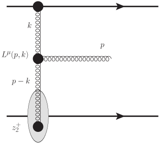
Figure 1: Fusion of the fields of two high-energy projectile and
target charges described by the Lipatov vertex.
Our result for the Lipatov vertex (in light-cone gauge A + = 0 superscript 𝐴 0 A^{+}=0
L i ( p , k ) = − 2 C i ( p , k ) k 2 { 1 + i 2 p 2 z 2 + p + − 1 8 ( p 2 z 2 + p + ) 2 } , superscript 𝐿 𝑖 𝑝 𝑘 2 superscript 𝐶 𝑖 𝑝 𝑘 superscript 𝑘 2 1 𝑖 2 superscript 𝑝 2 superscript subscript 𝑧 2 superscript 𝑝 1 8 superscript superscript 𝑝 2 superscript subscript 𝑧 2 superscript 𝑝 2 \displaystyle L^{i}(p,k)=-2C^{i}(p,k)\;k^{2}\left\{1+\frac{i}{2}p^{2}\frac{z_{2}^{+}}{p^{+}}-\frac{1}{8}\left(p^{2}\frac{z_{2}^{+}}{p^{+}}\right)^{2}\right\}~{}, (6)
where
C i ( p , k ) = p i p 2 − k i k 2 . superscript 𝐶 𝑖 𝑝 𝑘 superscript 𝑝 𝑖 superscript 𝑝 2 superscript 𝑘 𝑖 superscript 𝑘 2 C^{i}(p,k)=\frac{p^{i}}{p^{2}}-\frac{k^{i}}{k^{2}}~{}. (7)
A derivation is given in appendix A 1 6 ℓ + superscript ℓ \ell^{+} z 2 + / p + superscript subscript 𝑧 2 superscript 𝑝 z_{2}^{+}/p^{+} z 2 + / p + superscript subscript 𝑧 2 superscript 𝑝 z_{2}^{+}/p^{+} Altinoluk:2015gia
The vertex from eq. (6
ℳ λ a ( p ) = ϵ λ i p 2 A i , a ( p ) , subscript superscript ℳ 𝑎 𝜆 𝑝 superscript subscript italic-ϵ 𝜆 𝑖 superscript 𝑝 2 superscript 𝐴 𝑖 𝑎
𝑝 {\cal M}^{a}_{\lambda}(p)=\epsilon_{\lambda}^{i}\,p^{2}A^{i,a}(p)~{}, (8)
with p 2 A i , a ( p ) superscript 𝑝 2 superscript 𝐴 𝑖 𝑎
𝑝 p^{2}A^{i,a}(p) 1
To compute the single inclusive cross section we multiply
eq. (8 MV
S MV [ ρ ] = ∫ d 2 x ⟂ ∫ 0 ℓ + 𝑑 x + tr ρ ( x + , x ⟂ ) ρ ( x + , x ⟂ ) μ 2 , subscript 𝑆 MV delimited-[] 𝜌 superscript 𝑑 2 subscript 𝑥 perpendicular-to superscript subscript 0 superscript ℓ differential-d superscript 𝑥 tr 𝜌 superscript 𝑥 subscript 𝑥 perpendicular-to 𝜌 superscript 𝑥 subscript 𝑥 perpendicular-to superscript 𝜇 2 S_{\rm MV}[\rho]=\int d^{2}x_{\perp}\int\limits_{0}^{\ell^{+}}dx^{+}\;\frac{{\rm tr}\,\rho(x^{+},x_{\perp})\rho(x^{+},x_{\perp})}{\mu^{2}}~{}, (9)
which leads to the following color charge
correlator:
⟨ ρ a ( z 1 + , k 1 ) ρ ∗ b ( z 2 + , k 2 ) ⟩ = δ a b δ ( z 1 + − z 2 + ) ( 2 π ) 2 δ 2 ( k 1 − k 2 ) μ 2 . delimited-⟨⟩ superscript 𝜌 𝑎 superscript subscript 𝑧 1 subscript 𝑘 1 superscript 𝜌 absent 𝑏 superscript subscript 𝑧 2 subscript 𝑘 2 superscript 𝛿 𝑎 𝑏 𝛿 superscript subscript 𝑧 1 superscript subscript 𝑧 2 superscript 2 𝜋 2 superscript 𝛿 2 subscript 𝑘 1 subscript 𝑘 2 superscript 𝜇 2 \left<\rho^{a}(z_{1}^{+},k_{1})\,\rho^{*b}(z_{2}^{+},k_{2})\right>=\delta^{ab}\,\delta(z_{1}^{+}-z_{2}^{+})\,(2\pi)^{2}\delta^{2}(k_{1}-k_{2})\,\mu^{2}~{}. (10)
μ 2 superscript 𝜇 2 \mu^{2} z + superscript 𝑧 z^{+} 6 8
One may also consider a generalization of the MV-model action where
the two color charge densities sit at different longitudinal
coordinates,
S eff [ ρ ] = ∫ d 2 x ⟂ ∫ 0 ℓ + 𝑑 x + ∫ x + − λ + x + + λ + d y + 2 λ + tr ρ ( x + , x ⟂ ) U x + → y + ρ ( y + , x ⟂ ) U y + → x + μ 2 , subscript 𝑆 eff delimited-[] 𝜌 superscript 𝑑 2 subscript 𝑥 perpendicular-to superscript subscript 0 superscript ℓ differential-d superscript 𝑥 superscript subscript superscript 𝑥 superscript 𝜆 superscript 𝑥 superscript 𝜆 𝑑 superscript 𝑦 2 superscript 𝜆 tr 𝜌 superscript 𝑥 subscript 𝑥 perpendicular-to subscript 𝑈 → superscript 𝑥 superscript 𝑦 𝜌 superscript 𝑦 subscript 𝑥 perpendicular-to subscript 𝑈 → superscript 𝑦 superscript 𝑥 superscript 𝜇 2 S_{\rm eff}[\rho]=\int d^{2}x_{\perp}\int\limits_{0}^{\ell^{+}}dx^{+}\int\limits_{x^{+}-\lambda^{+}}^{x^{+}+\lambda^{+}}\frac{dy^{+}}{2\lambda^{+}}\frac{{\rm tr}\,\rho(x^{+},x_{\perp})U_{x^{+}\to y^{+}}\rho(y^{+},x_{\perp})U_{y^{+}\to x^{+}}}{\mu^{2}}~{}, (11)
and are connected by gauge links along the longitudinal
axis. λ + superscript 𝜆 \lambda^{+}
At leading order in g A − 𝑔 superscript 𝐴 gA^{-}
⟨ ρ a ( z 1 + , k 1 ) ρ ∗ b ( z 2 + , k 2 ) ⟩ = δ a b Θ ( λ + − | z 1 + − z 2 + | ) 1 2 λ + ( 2 π ) 2 δ 2 ( k 1 − k 2 ) μ 2 . delimited-⟨⟩ superscript 𝜌 𝑎 superscript subscript 𝑧 1 subscript 𝑘 1 superscript 𝜌 absent 𝑏 superscript subscript 𝑧 2 subscript 𝑘 2 superscript 𝛿 𝑎 𝑏 Θ superscript 𝜆 superscript subscript 𝑧 1 superscript subscript 𝑧 2 1 2 superscript 𝜆 superscript 2 𝜋 2 superscript 𝛿 2 subscript 𝑘 1 subscript 𝑘 2 superscript 𝜇 2 \left<\rho^{a}(z_{1}^{+},k_{1})\,\rho^{*b}(z_{2}^{+},k_{2})\right>=\delta^{ab}\,\Theta(\lambda^{+}-|z_{1}^{+}-z_{2}^{+}|)\frac{1}{2\lambda^{+}}\,(2\pi)^{2}\delta^{2}(k_{1}-k_{2})\,\mu^{2}~{}. (12)
This correlator reduces to the MV-model one from
eq. (10 λ + → 0 → superscript 𝜆 0 \lambda^{+}\to 0
In appendix B 12
p + d σ d p + d 2 p d 2 b superscript 𝑝 𝑑 𝜎 𝑑 superscript 𝑝 superscript 𝑑 2 𝑝 superscript 𝑑 2 𝑏 \displaystyle p^{+}\frac{d\sigma}{dp^{+}d^{2}p\,d^{2}b} = \displaystyle= 4 N c ( N c 2 − 1 ) S ⟂ g 2 p 2 [ 1 − 1 6 ( p 2 λ + 2 p + ) 2 ] ∫ d 2 k ( 2 π ) 2 Φ P ( k 2 ) Φ T ( ( p − k ) 2 ) . 4 subscript 𝑁 𝑐 superscript subscript 𝑁 𝑐 2 1 subscript 𝑆 perpendicular-to superscript 𝑔 2 superscript 𝑝 2 delimited-[] 1 1 6 superscript superscript 𝑝 2 superscript 𝜆 2 superscript 𝑝 2 superscript 𝑑 2 𝑘 superscript 2 𝜋 2 subscript Φ 𝑃 superscript 𝑘 2 subscript Φ 𝑇 superscript 𝑝 𝑘 2 \displaystyle 4N_{c}(N_{c}^{2}-1)\,S_{\perp}\frac{g^{2}}{p^{2}}\left[1-\frac{1}{6}\left(\frac{p^{2}\;\lambda^{+}}{2p^{+}}\right)^{2}\right]\int\frac{d^{2}k}{(2\pi)^{2}}\,\Phi_{P}(k^{2})\,\Phi_{T}((p-k)^{2})~{}. (13)
Here, S ⟂ subscript 𝑆 perpendicular-to S_{\perp} 13
Φ T ( k 2 ) = g 2 ℓ + μ T 2 k 2 , subscript Φ 𝑇 superscript 𝑘 2 superscript 𝑔 2 superscript ℓ superscript subscript 𝜇 𝑇 2 superscript 𝑘 2 \Phi_{T}(k^{2})=g^{2}\ell^{+}\,\frac{\mu_{T}^{2}}{k^{2}}~{}, (14)
and similar for the projectile. This function is dimensionless and
proportional to the saturation momentum squared, Q s 2 ∼ g 4 ℓ + μ 2 similar-to superscript subscript 𝑄 𝑠 2 superscript 𝑔 4 superscript ℓ superscript 𝜇 2 Q_{s}^{2}\sim g^{4}\ell^{+}\mu^{2} k 2 superscript 𝑘 2 k^{2} 14 ∼ 1 / k 2 similar-to absent 1 superscript 𝑘 2 \sim 1/k^{2}
We note that in eq. (13 ∼ p 2 λ + / p + similar-to absent superscript 𝑝 2 superscript 𝜆 superscript 𝑝 \sim p^{2}\lambda^{+}/p^{+} Altinoluk:2014oxa ; Altinoluk:2015gia B p + superscript 𝑝 p^{+} λ + superscript 𝜆 \lambda^{+} ℓ + superscript ℓ \ell^{+} z 2 + superscript subscript 𝑧 2 z_{2}^{+} z ¯ 2 + superscript subscript ¯ 𝑧 2 \bar{z}_{2}^{+} λ + superscript 𝜆 \lambda^{+}
Next, we consider two gluon inclusive production. A detailed
derivation is provided in appendix C
Figure 2: Double inclusive gluon production
In the linear approximation two gluon production corresponds to the
diagram shown in fig. 2 Dumitru:2008wn ℓ + ∼ A 1 / 3 similar-to superscript ℓ superscript 𝐴 1 3 \ell^{+}\sim A^{1/3} z + superscript 𝑧 z^{+} 9 10 C ρ 1 subscript 𝜌 1 \rho_{1} ρ 2 ∗ superscript subscript 𝜌 2 \rho_{2}^{*} ρ 1 ∗ superscript subscript 𝜌 1 \rho_{1}^{*} ρ 2 subscript 𝜌 2 \rho_{2} C ρ 1 subscript 𝜌 1 \rho_{1} ρ 2 subscript 𝜌 2 \rho_{2} ρ 1 ∗ superscript subscript 𝜌 1 \rho_{1}^{*} ρ 2 ∗ superscript subscript 𝜌 2 \rho_{2}^{*} C
( ℓ + p 2 p + ) 2 superscript superscript ℓ superscript 𝑝 2 superscript 𝑝 2 \left(\frac{\ell^{+}\,p^{2}}{p^{+}}\right)^{2} (15)
which is proportional to A 2 / 3 superscript 𝐴 2 3 A^{2/3}
p + q + d σ d p + d 2 p d q + d 2 q superscript 𝑝 superscript 𝑞 𝑑 𝜎 𝑑 superscript 𝑝 superscript 𝑑 2 𝑝 𝑑 superscript 𝑞 superscript 𝑑 2 𝑞 \displaystyle p^{+}q^{+}\frac{d\sigma}{dp^{+}d^{2}pdq^{+}d^{2}q} = \displaystyle= 16 N c 2 ( N c 2 − 1 ) g 4 S ⟂ p 2 q 2 ∫ d 2 k 1 ( 2 π ) 2 d 2 k 2 ( 2 π ) 2 Φ P ( k 1 2 ) Φ P ( k 2 2 ) Φ T [ ( p − k 1 ) 2 ] Φ T [ ( q − k 2 ) 2 ] 16 superscript subscript 𝑁 𝑐 2 superscript subscript 𝑁 𝑐 2 1 superscript 𝑔 4 subscript 𝑆 perpendicular-to superscript 𝑝 2 superscript 𝑞 2 superscript 𝑑 2 subscript 𝑘 1 superscript 2 𝜋 2 superscript 𝑑 2 subscript 𝑘 2 superscript 2 𝜋 2 subscript Φ 𝑃 superscript subscript 𝑘 1 2 subscript Φ 𝑃 superscript subscript 𝑘 2 2 subscript Φ 𝑇 delimited-[] superscript 𝑝 subscript 𝑘 1 2 subscript Φ 𝑇 delimited-[] superscript 𝑞 subscript 𝑘 2 2 \displaystyle 16N_{c}^{2}(N_{c}^{2}-1)\,g^{4}\frac{S_{\perp}}{p^{2}q^{2}}\int\frac{d^{2}k_{1}}{(2\pi)^{2}}\frac{d^{2}k_{2}}{(2\pi)^{2}}\Phi_{P}(k_{1}^{2})\Phi_{P}(k_{2}^{2})\Phi_{T}\big{[}(p-k_{1})^{2}\big{]}\Phi_{T}\big{[}(q-k_{2})^{2}\big{]} (16)
[ δ ( 2 ) ( k 1 + k 2 ) + δ ( 2 ) ( k 1 − k 2 ) \displaystyle\left[\delta^{(2)}(k_{1}+k_{2})+\delta^{(2)}(k_{1}-k_{2})\right.
+ \displaystyle+ 1 8 δ ( 2 ) ( p − q − k 1 + k 2 ) [ 1 − 1 12 ( p 2 2 p + − q 2 2 q + ) 2 ℓ + 2 ] 1 8 superscript 𝛿 2 𝑝 𝑞 subscript 𝑘 1 subscript 𝑘 2 delimited-[] 1 1 12 superscript superscript 𝑝 2 2 superscript 𝑝 superscript 𝑞 2 2 superscript 𝑞 2 superscript superscript ℓ 2 \displaystyle\frac{1}{8}\delta^{(2)}(p-q-k_{1}+k_{2})\left[1-\frac{1}{12}\left(\frac{p^{2}}{2p^{+}}-\frac{q^{2}}{2q^{+}}\right)^{2}{\ell^{+}}^{2}\right]
× { 1 + k 2 2 ( p − k 1 ) 2 k 1 2 ( p + k 2 ) 2 − p 2 ( k 1 + k 2 ) 2 k 1 2 ( p + k 2 ) 2 } { 1 + k 1 2 ( q − k 2 ) 2 k 2 2 ( q + k 1 ) 2 − q 2 ( k 1 + k 2 ) 2 k 2 2 ( q + k 1 ) 2 } absent 1 superscript subscript 𝑘 2 2 superscript 𝑝 subscript 𝑘 1 2 superscript subscript 𝑘 1 2 superscript 𝑝 subscript 𝑘 2 2 superscript 𝑝 2 superscript subscript 𝑘 1 subscript 𝑘 2 2 superscript subscript 𝑘 1 2 superscript 𝑝 subscript 𝑘 2 2 1 superscript subscript 𝑘 1 2 superscript 𝑞 subscript 𝑘 2 2 superscript subscript 𝑘 2 2 superscript 𝑞 subscript 𝑘 1 2 superscript 𝑞 2 superscript subscript 𝑘 1 subscript 𝑘 2 2 superscript subscript 𝑘 2 2 superscript 𝑞 subscript 𝑘 1 2 \displaystyle\left.\times\left\{1+\frac{k_{2}^{2}(p-k_{1})^{2}}{k_{1}^{2}(p+k_{2})^{2}}-\frac{p^{2}(k_{1}+k_{2})^{2}}{k_{1}^{2}(p+k_{2})^{2}}\right\}\left\{1+\frac{k_{1}^{2}(q-k_{2})^{2}}{k_{2}^{2}(q+k_{1})^{2}}-\frac{q^{2}(k_{1}+k_{2})^{2}}{k_{2}^{2}(q+k_{1})^{2}}\right\}\right.
+ \displaystyle+ 1 4 δ ( 2 ) ( p − q ) [ 1 − 1 12 ( p 2 2 p + − q 2 2 q + ) 2 ℓ + 2 ] 1 4 superscript 𝛿 2 𝑝 𝑞 delimited-[] 1 1 12 superscript superscript 𝑝 2 2 superscript 𝑝 superscript 𝑞 2 2 superscript 𝑞 2 superscript superscript ℓ 2 \displaystyle\frac{1}{4}\delta^{(2)}(p-q)\left[1-\frac{1}{12}\left(\frac{p^{2}}{2p^{+}}-\frac{q^{2}}{2q^{+}}\right)^{2}{\ell^{+}}^{2}\right]
× { 1 + k 2 2 ( p − k 1 ) 2 k 1 2 ( p − k 2 ) 2 − p 2 ( k 1 − k 2 ) 2 k 1 2 ( p − k 2 ) 2 } { 1 + k 1 2 ( q − k 2 ) 2 k 2 2 ( q − k 1 ) 2 − q 2 ( k 1 − k 2 ) 2 k 2 2 ( q − k 1 ) 2 } absent 1 superscript subscript 𝑘 2 2 superscript 𝑝 subscript 𝑘 1 2 superscript subscript 𝑘 1 2 superscript 𝑝 subscript 𝑘 2 2 superscript 𝑝 2 superscript subscript 𝑘 1 subscript 𝑘 2 2 superscript subscript 𝑘 1 2 superscript 𝑝 subscript 𝑘 2 2 1 superscript subscript 𝑘 1 2 superscript 𝑞 subscript 𝑘 2 2 superscript subscript 𝑘 2 2 superscript 𝑞 subscript 𝑘 1 2 superscript 𝑞 2 superscript subscript 𝑘 1 subscript 𝑘 2 2 superscript subscript 𝑘 2 2 superscript 𝑞 subscript 𝑘 1 2 \displaystyle\left.\times\left\{1+\frac{k_{2}^{2}(p-k_{1})^{2}}{k_{1}^{2}(p-k_{2})^{2}}-\frac{p^{2}(k_{1}-k_{2})^{2}}{k_{1}^{2}(p-k_{2})^{2}}\right\}\left\{1+\frac{k_{1}^{2}(q-k_{2})^{2}}{k_{2}^{2}(q-k_{1})^{2}}-\frac{q^{2}(k_{1}-k_{2})^{2}}{k_{2}^{2}(q-k_{1})^{2}}\right\}\right.
+ \displaystyle+ δ ( 2 ) ( p − q − k 1 + k 2 ) [ 1 − 1 12 ( p 2 2 p + − q 2 2 q + ) 2 ℓ + 2 ] superscript 𝛿 2 𝑝 𝑞 subscript 𝑘 1 subscript 𝑘 2 delimited-[] 1 1 12 superscript superscript 𝑝 2 2 superscript 𝑝 superscript 𝑞 2 2 superscript 𝑞 2 superscript superscript ℓ 2 \displaystyle\delta^{(2)}(p-q-k_{1}+k_{2})\left[1-\frac{1}{12}\left(\frac{p^{2}}{2p^{+}}-\frac{q^{2}}{2q^{+}}\right)^{2}{\ell^{+}}^{2}\right]
+ \displaystyle+ 1 4 δ ( 2 ) ( p + q ) [ 1 − 1 12 ( p 2 2 p + + q 2 2 q + ) 2 ℓ + 2 ] 1 4 superscript 𝛿 2 𝑝 𝑞 delimited-[] 1 1 12 superscript superscript 𝑝 2 2 superscript 𝑝 superscript 𝑞 2 2 superscript 𝑞 2 superscript superscript ℓ 2 \displaystyle\frac{1}{4}\delta^{(2)}(p+q)\left[1-\frac{1}{12}\left(\frac{p^{2}}{2p^{+}}+\frac{q^{2}}{2q^{+}}\right)^{2}{\ell^{+}}^{2}\right]
× { 1 + k 2 2 ( p − k 1 ) 2 k 1 2 ( p + k 2 ) 2 − p 2 ( k 1 + k 2 ) 2 k 1 2 ( p + k 2 ) 2 } { 1 + k 1 2 ( q − k 2 ) 2 k 2 2 ( q + k 1 ) 2 − q 2 ( k 1 + k 2 ) 2 k 2 2 ( q + k 1 ) 2 } absent 1 superscript subscript 𝑘 2 2 superscript 𝑝 subscript 𝑘 1 2 superscript subscript 𝑘 1 2 superscript 𝑝 subscript 𝑘 2 2 superscript 𝑝 2 superscript subscript 𝑘 1 subscript 𝑘 2 2 superscript subscript 𝑘 1 2 superscript 𝑝 subscript 𝑘 2 2 1 superscript subscript 𝑘 1 2 superscript 𝑞 subscript 𝑘 2 2 superscript subscript 𝑘 2 2 superscript 𝑞 subscript 𝑘 1 2 superscript 𝑞 2 superscript subscript 𝑘 1 subscript 𝑘 2 2 superscript subscript 𝑘 2 2 superscript 𝑞 subscript 𝑘 1 2 \displaystyle\times\left\{1+\frac{k_{2}^{2}(p-k_{1})^{2}}{k_{1}^{2}(p+k_{2})^{2}}-\frac{p^{2}(k_{1}+k_{2})^{2}}{k_{1}^{2}(p+k_{2})^{2}}\right\}\left\{1+\frac{k_{1}^{2}(q-k_{2})^{2}}{k_{2}^{2}(q+k_{1})^{2}}-\frac{q^{2}(k_{1}+k_{2})^{2}}{k_{2}^{2}(q+k_{1})^{2}}\right\}
+ \displaystyle+ 1 8 δ ( 2 ) ( p + q − k 1 − k 2 ) [ 1 − 1 12 ( p 2 2 p + + q 2 2 q + ) 2 ℓ + 2 ] 1 8 superscript 𝛿 2 𝑝 𝑞 subscript 𝑘 1 subscript 𝑘 2 delimited-[] 1 1 12 superscript superscript 𝑝 2 2 superscript 𝑝 superscript 𝑞 2 2 superscript 𝑞 2 superscript superscript ℓ 2 \displaystyle\frac{1}{8}\delta^{(2)}(p+q-k_{1}-k_{2})\left[1-\frac{1}{12}\left(\frac{p^{2}}{2p^{+}}+\frac{q^{2}}{2q^{+}}\right)^{2}{\ell^{+}}^{2}\right]
× { 1 + k 2 2 ( p − k 1 ) 2 k 1 2 ( p − k 2 ) 2 − p 2 ( k 1 − k 2 ) 2 k 1 2 ( p − k 2 ) 2 } { 1 + k 1 2 ( q − k 2 ) 2 k 2 2 ( q − k 1 ) 2 − q 2 ( k 1 − k 2 ) 2 k 2 2 ( q − k 1 ) 2 } absent 1 superscript subscript 𝑘 2 2 superscript 𝑝 subscript 𝑘 1 2 superscript subscript 𝑘 1 2 superscript 𝑝 subscript 𝑘 2 2 superscript 𝑝 2 superscript subscript 𝑘 1 subscript 𝑘 2 2 superscript subscript 𝑘 1 2 superscript 𝑝 subscript 𝑘 2 2 1 superscript subscript 𝑘 1 2 superscript 𝑞 subscript 𝑘 2 2 superscript subscript 𝑘 2 2 superscript 𝑞 subscript 𝑘 1 2 superscript 𝑞 2 superscript subscript 𝑘 1 subscript 𝑘 2 2 superscript subscript 𝑘 2 2 superscript 𝑞 subscript 𝑘 1 2 \displaystyle\times\left\{1+\frac{k_{2}^{2}(p-k_{1})^{2}}{k_{1}^{2}(p-k_{2})^{2}}-\frac{p^{2}(k_{1}-k_{2})^{2}}{k_{1}^{2}(p-k_{2})^{2}}\right\}\left\{1+\frac{k_{1}^{2}(q-k_{2})^{2}}{k_{2}^{2}(q-k_{1})^{2}}-\frac{q^{2}(k_{1}-k_{2})^{2}}{k_{2}^{2}(q-k_{1})^{2}}\right\}
+ \displaystyle+ δ ( 2 ) ( p + q − k 1 − k 2 ) [ 1 − 1 12 ( p 2 2 p + + q 2 2 q + ) 2 ℓ + 2 ] superscript 𝛿 2 𝑝 𝑞 subscript 𝑘 1 subscript 𝑘 2 delimited-[] 1 1 12 superscript superscript 𝑝 2 2 superscript 𝑝 superscript 𝑞 2 2 superscript 𝑞 2 superscript superscript ℓ 2 \displaystyle\delta^{(2)}(p+q-k_{1}-k_{2})\left[1-\frac{1}{12}\left(\frac{p^{2}}{2p^{+}}+\frac{q^{2}}{2q^{+}}\right)^{2}{\ell^{+}}^{2}\right]
] . ] \displaystyle\Big{]}~{}.
This expression does not include the disconnected contribution
corresponding to uncorrelated production of the two gluons.
The fact that NNE corrections do appear in the two-gluon cross section
and that they are not the same for all diagrams could be important for
studies of two-particle azimuthal correlations. However, more detailed
computations with realistic unintegrated gluon densities, and
including the dijet contribution are
required DuslingVenugopalan
In summary, in this paper we have evaluated explicitly Wilson lines
with electric field insertions to leading order in the field g A − 𝑔 superscript 𝐴 gA^{-} A 1 / 3 superscript 𝐴 1 3 A^{1/3} k T subscript 𝑘 𝑇 k_{T} z + superscript 𝑧 z^{+} ℓ + p 2 / p + superscript ℓ superscript 𝑝 2 superscript 𝑝 \ell^{+}\,p^{2}/p^{+}
Acknowledgements.
T.A. expresses his gratitude to the Department of Natural Sciences of
Baruch College for their warm hospitality during a visit when this
work was done. T.A. acknowledges
support by
the People Programme (Marie Curie Actions) of the European Union’s
Seventh Framework Programme FP7/2007-2013/ under REA grant agreement #318921;
the European Research Council grant
HotLHC ERC-2011-StG-279579, Ministerio de Ciencia e Innovación of
Spain under project FPA2014-58293-C2-1-P, Xunta de Galicia
(Consellería de Educación and Consellería de Innovación e
Industria - Programa Incite),
the Spanish Consolider-Ingenio 2010 Programme CPAN and FEDER.
A.D. gratefully acknowledges support by the DOE
Office of Nuclear Physics through Grant No. DE-FG02-09ER41620; and
from The City University of New York through the PSC-CUNY Research
grants 67119-0045 and 69362-0047.
Appendix A The Lipatov vertex to NNE level
In this appendix we provide details of the calculation of NE and NNE
corrections to the Lipatov vertex. The gluon-nucleus reduced
amplitude at NNE accuracy
Altinoluk:2015gia
M ¯ λ a b ( p ¯ , k ) = i ε λ ∗ i ∫ d 2 x e i x ⋅ ( k − p ) { 2 C i ( p , k ) 𝒰 ( ℓ + , 0 ; x ) + ℓ + p + [ ( δ i j − 2 p j k i k 2 ) 𝒰 [ 0 , 1 ] j ( ℓ + , 0 ; x ) − i k i k 2 𝒰 [ 1 , 0 ] ( ℓ + , 0 ; x ) ] \displaystyle{\overline{M}}^{ab}_{\lambda}(\underline{p},k)=i\varepsilon^{*i}_{\lambda}\int d^{2}x\,e^{ix\cdot(k-p)}\Bigg{\{}2C^{i}(p,k)\,{\cal U}(\ell^{+},0;x)+\frac{\ell^{+}}{p^{+}}\left[\left(\delta^{ij}-2p^{j}\frac{k^{i}}{k^{2}}\right){\cal U}^{j}_{[0,1]}(\ell^{+},0;x)-i\frac{k^{i}}{k^{2}}{\cal U}_{[1,0]}(\ell^{+},0;x)\right]
+ ( ℓ + p + ) 2 [ − k i k 2 p j p l 𝒰 [ 0 , 2 ] j l ( ℓ + , 0 ; x ) − i k i k 2 p j 𝒰 [ 1 , 1 ] j ( ℓ + , 0 ; x ) + 1 2 k i k 2 𝒰 [ 2 , 0 ] ( ℓ + , 0 ; x ) \displaystyle~{}~{}~{}~{}~{}~{}~{}~{}~{}~{}~{}~{}~{}~{}~{}~{}~{}~{}~{}~{}~{}~{}+\left(\frac{\ell^{+}}{p^{+}}\right)^{2}\Bigg{[}-\frac{k^{i}}{k^{2}}p^{j}p^{l}{\cal U}^{jl}_{[0,2]}(\ell^{+},0;x)-i\frac{k^{i}}{k^{2}}p^{j}{\cal U}^{j}_{[1,1]}(\ell^{+},0;x)+\frac{1}{2}\frac{k^{i}}{k^{2}}{\cal U}_{[2,0]}(\ell^{+},0;x)
+ i 4 ( p 2 δ i j − 2 p i p j ) 𝒰 ( A ) j ( ℓ + , 0 ; x ) + 1 4 p j 𝒰 ( B ) i j ( ℓ + , 0 ; x ) + i 4 𝒰 ( C ) i ( ℓ + , 0 ; x ) ] } , \displaystyle~{}~{}~{}~{}~{}~{}~{}~{}~{}~{}~{}~{}~{}~{}~{}~{}~{}~{}~{}~{}~{}~{}+\frac{i}{4}\left(p^{2}\delta^{ij}-2p^{i}p^{j}\right){\cal U}^{j}_{({\rm A})}(\ell^{+},0;x)+\frac{1}{4}p^{j}{\cal U}^{ij}_{({\rm B})}(\ell^{+},0;x)+\frac{i}{4}{\cal U}^{i}_{({\rm C})}(\ell^{+},0;x)\Bigg{]}\Bigg{\}}\;, (17)
where ( p ¯ ) ≡ ( p + , p ) ¯ 𝑝 superscript 𝑝 𝑝 (\underline{p})\equiv(p^{+},p) g ρ T 𝑔 subscript 𝜌 𝑇 g\rho_{T}
∫ d 2 x e i x ⋅ ( k − p ) 𝒰 ( ℓ + , 0 ; x ) a b = ( 2 π ) 2 δ ( k − p ) 1 a b + i g 2 T c a b 1 ( p − k ) 2 ∫ 0 ℓ + 𝑑 z + ρ T c ( z + , p − k ) + O ( ρ T 2 ) . superscript 𝑑 2 𝑥 superscript 𝑒 ⋅ 𝑖 𝑥 𝑘 𝑝 𝒰 superscript superscript ℓ 0 𝑥 𝑎 𝑏 superscript 2 𝜋 2 𝛿 𝑘 𝑝 superscript 1 𝑎 𝑏 𝑖 superscript 𝑔 2 subscript superscript 𝑇 𝑎 𝑏 𝑐 1 superscript 𝑝 𝑘 2 superscript subscript 0 superscript ℓ differential-d superscript 𝑧 superscript subscript 𝜌 𝑇 𝑐 superscript 𝑧 𝑝 𝑘 𝑂 superscript subscript 𝜌 𝑇 2 \int d^{2}x\,e^{ix\cdot(k-p)}{\cal U}(\ell^{+},0;x)^{ab}=(2\pi)^{2}\delta(k-p)1^{ab}+i\,g^{2}T^{ab}_{c}\frac{1}{(p-k)^{2}}\int_{0}^{\ell^{+}}dz^{+}\rho_{T}^{c}(z^{+},p-k)+O(\rho_{T}^{2}). (18)
The decorated Wilson lines that appear at NE and NNE level are
Wilson lines with one or more background field insertions
along the longitudinal axis from 0 0 ℓ + superscript ℓ \ell^{+} Altinoluk:2015gia ρ T subscript 𝜌 𝑇 \rho_{T} ρ T subscript 𝜌 𝑇 \rho_{T}
∫ d 2 x e i x ⋅ ( k − p ) 𝒰 [ 0 , 1 ] j ( ℓ + , 0 , x ) a b = − g 2 T c a b ( p − k ) j ( p − k ) 2 ∫ 0 ℓ + 𝑑 z + ( z + ℓ + ) ρ T c ( z + , p − k ) + O ( ρ T 2 ) superscript 𝑑 2 𝑥 superscript 𝑒 ⋅ 𝑖 𝑥 𝑘 𝑝 subscript superscript 𝒰 𝑗 0 1 superscript superscript ℓ 0 𝑥 𝑎 𝑏 superscript 𝑔 2 subscript superscript 𝑇 𝑎 𝑏 𝑐 superscript 𝑝 𝑘 𝑗 superscript 𝑝 𝑘 2 superscript subscript 0 superscript ℓ differential-d superscript 𝑧 superscript 𝑧 superscript ℓ subscript superscript 𝜌 𝑐 𝑇 superscript 𝑧 𝑝 𝑘 𝑂 subscript superscript 𝜌 2 𝑇 \int d^{2}x\,e^{ix\cdot(k-p)}{\cal U}^{j}_{[0,1]}(\ell^{+},0,x)^{ab}=-g^{2}T^{ab}_{c}\frac{(p-k)^{j}}{(p-k)^{2}}\int_{0}^{\ell^{+}}dz^{+}\left(\frac{z^{+}}{\ell^{+}}\right)\rho^{c}_{T}(z^{+},p-k)+O(\rho^{2}_{T}) (19)
∫ d 2 x e i x ⋅ ( k − p ) 𝒰 [ 1 , 0 ] ( ℓ + , 0 , x ) a b = − i g 2 T c a b ∫ 0 ℓ + 𝑑 z + ( z + ℓ + ) ρ T c ( z + , p − k ) + O ( ρ T 2 ) superscript 𝑑 2 𝑥 superscript 𝑒 ⋅ 𝑖 𝑥 𝑘 𝑝 subscript 𝒰 1 0 superscript superscript ℓ 0 𝑥 𝑎 𝑏 𝑖 superscript 𝑔 2 subscript superscript 𝑇 𝑎 𝑏 𝑐 superscript subscript 0 superscript ℓ differential-d superscript 𝑧 superscript 𝑧 superscript ℓ subscript superscript 𝜌 𝑐 𝑇 superscript 𝑧 𝑝 𝑘 𝑂 subscript superscript 𝜌 2 𝑇 \int d^{2}x\,e^{ix\cdot(k-p)}{\cal U}_{[1,0]}(\ell^{+},0,x)^{ab}=-ig^{2}T^{ab}_{c}\int_{0}^{\ell^{+}}dz^{+}\left(\frac{z^{+}}{\ell^{+}}\right)\rho^{c}_{T}(z^{+},p-k)+O(\rho^{2}_{T}) (20)
∫ d 2 x e i x ⋅ ( k − p ) 𝒰 [ 0 , 2 ] j l ( ℓ + , 0 , x ) a b = − i g 2 T c a b ( p − k ) j ( p − k ) l ( p − k ) 2 ∫ 0 ℓ + 𝑑 z + ( z + ℓ + ) 2 ρ T c ( z + , p − k ) + O ( ρ T 2 ) superscript 𝑑 2 𝑥 superscript 𝑒 ⋅ 𝑖 𝑥 𝑘 𝑝 subscript superscript 𝒰 𝑗 𝑙 0 2 superscript superscript ℓ 0 𝑥 𝑎 𝑏 𝑖 superscript 𝑔 2 subscript superscript 𝑇 𝑎 𝑏 𝑐 superscript 𝑝 𝑘 𝑗 superscript 𝑝 𝑘 𝑙 superscript 𝑝 𝑘 2 superscript subscript 0 superscript ℓ differential-d superscript 𝑧 superscript superscript 𝑧 superscript ℓ 2 subscript superscript 𝜌 𝑐 𝑇 superscript 𝑧 𝑝 𝑘 𝑂 subscript superscript 𝜌 2 𝑇 \int d^{2}x\,e^{ix\cdot(k-p)}{\cal U}^{jl}_{[0,2]}(\ell^{+},0,x)^{ab}=-ig^{2}T^{ab}_{c}\frac{(p-k)^{j}(p-k)^{l}}{(p-k)^{2}}\int_{0}^{\ell^{+}}dz^{+}\left(\frac{z^{+}}{\ell^{+}}\right)^{2}\rho^{c}_{T}(z^{+},p-k)+O(\rho^{2}_{T}) (21)
∫ d 2 x e i x ⋅ ( k − p ) 𝒰 [ 1 , 1 ] j ( ℓ + , 0 , x ) a b = g 2 T c a b ( p − k ) j ∫ 0 ℓ + 𝑑 z + ( z + ℓ + ) 2 ρ T c ( z + , p − k ) + O ( ρ T 2 ) superscript 𝑑 2 𝑥 superscript 𝑒 ⋅ 𝑖 𝑥 𝑘 𝑝 subscript superscript 𝒰 𝑗 1 1 superscript superscript ℓ 0 𝑥 𝑎 𝑏 superscript 𝑔 2 subscript superscript 𝑇 𝑎 𝑏 𝑐 superscript 𝑝 𝑘 𝑗 superscript subscript 0 superscript ℓ differential-d superscript 𝑧 superscript superscript 𝑧 superscript ℓ 2 subscript superscript 𝜌 𝑐 𝑇 superscript 𝑧 𝑝 𝑘 𝑂 subscript superscript 𝜌 2 𝑇 \int d^{2}x\,e^{ix\cdot(k-p)}{\cal U}^{j}_{[1,1]}(\ell^{+},0,x)^{ab}=g^{2}T^{ab}_{c}(p-k)^{j}\int_{0}^{\ell^{+}}dz^{+}\left(\frac{z^{+}}{\ell^{+}}\right)^{2}\rho^{c}_{T}(z^{+},p-k)+O(\rho^{2}_{T}) (22)
∫ d 2 x e i x ⋅ ( k − p ) 𝒰 [ 2 , 0 ] ( ℓ + , 0 , x ) a b = i g 2 T c a b ( p − k ) 2 1 2 ∫ 0 ℓ + 𝑑 z + ( z + ℓ + ) 2 ρ T c ( z + , p − k ) + O ( ρ T 2 ) superscript 𝑑 2 𝑥 superscript 𝑒 ⋅ 𝑖 𝑥 𝑘 𝑝 subscript 𝒰 2 0 superscript superscript ℓ 0 𝑥 𝑎 𝑏 𝑖 superscript 𝑔 2 subscript superscript 𝑇 𝑎 𝑏 𝑐 superscript 𝑝 𝑘 2 1 2 superscript subscript 0 superscript ℓ differential-d superscript 𝑧 superscript superscript 𝑧 superscript ℓ 2 subscript superscript 𝜌 𝑐 𝑇 superscript 𝑧 𝑝 𝑘 𝑂 subscript superscript 𝜌 2 𝑇 \displaystyle\int d^{2}x\,e^{ix\cdot(k-p)}{\cal U}_{[2,0]}(\ell^{+},0,x)^{ab}=ig^{2}T^{ab}_{c}(p-k)^{2}\frac{1}{2}\int_{0}^{\ell^{+}}dz^{+}\left(\frac{z^{+}}{\ell^{+}}\right)^{2}\rho^{c}_{T}(z^{+},p-k)+O(\rho^{2}_{T}) (23)
∫ d 2 x e i x ⋅ ( k − p ) 𝒰 ( A ) j ( ℓ + , 0 , x ) a b = − g 2 T c a b ( p − k ) j ( p − k ) 2 ∫ 0 ℓ + 𝑑 z + ( z + ℓ + ) 2 ρ T c ( z + , p − k ) + O ( ρ T 2 ) superscript 𝑑 2 𝑥 superscript 𝑒 ⋅ 𝑖 𝑥 𝑘 𝑝 subscript superscript 𝒰 𝑗 A superscript superscript ℓ 0 𝑥 𝑎 𝑏 superscript 𝑔 2 subscript superscript 𝑇 𝑎 𝑏 𝑐 superscript 𝑝 𝑘 𝑗 superscript 𝑝 𝑘 2 superscript subscript 0 superscript ℓ differential-d superscript 𝑧 superscript superscript 𝑧 superscript ℓ 2 subscript superscript 𝜌 𝑐 𝑇 superscript 𝑧 𝑝 𝑘 𝑂 subscript superscript 𝜌 2 𝑇 \displaystyle\int d^{2}x\,e^{ix\cdot(k-p)}{\cal U}^{j}_{({\rm A})}(\ell^{+},0,x)^{ab}=-g^{2}T^{ab}_{c}\frac{(p-k)^{j}}{(p-k)^{2}}\int_{0}^{\ell^{+}}dz^{+}\left(\frac{z^{+}}{\ell^{+}}\right)^{2}\rho^{c}_{T}(z^{+},p-k)+O(\rho^{2}_{T}) (24)
∫ d 2 x e i x ⋅ ( k − p ) 𝒰 ( B ) i j ( ℓ + , 0 , x ) a b = − i g 2 T c a b [ δ i j δ l m + δ i l δ j m + δ i m δ j l ] ( p − k ) l ( p − k ) m ( p − k ) 2 superscript 𝑑 2 𝑥 superscript 𝑒 ⋅ 𝑖 𝑥 𝑘 𝑝 subscript superscript 𝒰 𝑖 𝑗 B superscript superscript ℓ 0 𝑥 𝑎 𝑏 𝑖 superscript 𝑔 2 subscript superscript 𝑇 𝑎 𝑏 𝑐 delimited-[] superscript 𝛿 𝑖 𝑗 superscript 𝛿 𝑙 𝑚 superscript 𝛿 𝑖 𝑙 superscript 𝛿 𝑗 𝑚 superscript 𝛿 𝑖 𝑚 superscript 𝛿 𝑗 𝑙 superscript 𝑝 𝑘 𝑙 superscript 𝑝 𝑘 𝑚 superscript 𝑝 𝑘 2 \displaystyle\int d^{2}x\,e^{ix\cdot(k-p)}{\cal U}^{ij}_{({\rm B})}(\ell^{+},0,x)^{ab}=-ig^{2}T^{ab}_{c}[\delta^{ij}\delta^{lm}+\delta^{il}\delta^{jm}+\delta^{im}\delta^{jl}]\frac{(p-k)^{l}(p-k)^{m}}{(p-k)^{2}}
× ∫ 0 ℓ + d z + ( z + ℓ + ) 2 ρ T c ( z + , p − k ) + O ( ρ T 2 ) \displaystyle~{}~{}~{}~{}~{}~{}~{}~{}~{}~{}~{}~{}~{}~{}~{}~{}~{}~{}~{}~{}~{}~{}~{}~{}~{}~{}~{}~{}~{}~{}~{}~{}~{}~{}~{}~{}~{}~{}~{}~{}~{}~{}\times\int_{0}^{\ell^{+}}dz^{+}\left(\frac{z^{+}}{\ell^{+}}\right)^{2}\rho^{c}_{T}(z^{+},p-k)+O(\rho^{2}_{T}) (25)
∫ d 2 x e i x ⋅ ( k − p ) 𝒰 ( C ) i ( ℓ + , 0 , x ) a b = g 2 T c a b ( p − k ) i ∫ 0 ℓ + 𝑑 z + ( z + ℓ + ) 2 ρ T c ( z + , p − k ) + O ( ρ T 2 ) superscript 𝑑 2 𝑥 superscript 𝑒 ⋅ 𝑖 𝑥 𝑘 𝑝 subscript superscript 𝒰 𝑖 C superscript superscript ℓ 0 𝑥 𝑎 𝑏 superscript 𝑔 2 subscript superscript 𝑇 𝑎 𝑏 𝑐 superscript 𝑝 𝑘 𝑖 superscript subscript 0 superscript ℓ differential-d superscript 𝑧 superscript superscript 𝑧 superscript ℓ 2 subscript superscript 𝜌 𝑐 𝑇 superscript 𝑧 𝑝 𝑘 𝑂 subscript superscript 𝜌 2 𝑇 \displaystyle\int d^{2}x\,e^{ix\cdot(k-p)}{\cal U}^{i}_{({\rm C})}(\ell^{+},0,x)^{ab}=g^{2}T^{ab}_{c}(p-k)^{i}\int_{0}^{\ell^{+}}dz^{+}\left(\frac{z^{+}}{\ell^{+}}\right)^{2}\rho^{c}_{T}(z^{+},p-k)+O(\rho^{2}_{T}) (26)
Using the expressions above, it is straightforward to obtain the
amplitude at order ρ T subscript 𝜌 𝑇 \rho_{T}
M ¯ λ a b ( p ¯ , k ) = i ε λ ∗ i ( i g 2 ) T c a b 1 ( p − k ) 2 ∫ 0 ℓ + 𝑑 z + 2 C i ( p , k ) { 1 + i 2 p 2 z + p + − 1 8 ( p 2 z + p + ) 2 } ρ T c ( z + , p − k ) . subscript superscript ¯ 𝑀 𝑎 𝑏 𝜆 ¯ 𝑝 𝑘 𝑖 subscript superscript 𝜀 absent 𝑖 𝜆 𝑖 superscript 𝑔 2 subscript superscript 𝑇 𝑎 𝑏 𝑐 1 superscript 𝑝 𝑘 2 superscript subscript 0 superscript ℓ differential-d superscript 𝑧 2 superscript 𝐶 𝑖 𝑝 𝑘 1 𝑖 2 superscript 𝑝 2 superscript 𝑧 superscript 𝑝 1 8 superscript superscript 𝑝 2 superscript 𝑧 superscript 𝑝 2 superscript subscript 𝜌 𝑇 𝑐 superscript 𝑧 𝑝 𝑘 {\overline{M}}^{ab}_{\lambda}(\underline{p},k)=i\varepsilon^{*i}_{\lambda}(ig^{2})T^{ab}_{c}\frac{1}{(p-k)^{2}}\int_{0}^{\ell^{+}}dz^{+}~{}2C^{i}(p,k)\Bigg{\{}1+\frac{i}{2}p^{2}\frac{z^{+}}{p^{+}}-\frac{1}{8}\left(p^{2}\frac{z^{+}}{p^{+}}\right)^{2}\Bigg{\}}\rho_{T}^{c}(z^{+},p-k)~{}. (27)
One can now read off the Lipatov vertex at NNE accuracy as written in
eq. (6 𝒪 ( ℓ + ) 𝒪 superscript ℓ {\cal O}(\ell^{+}) 𝒪 ( ℓ + 2 ) 𝒪 superscript ℓ 2 {\cal O}(\ell^{+2}) 27
{ 1 + i 2 p 2 z + p + − 1 8 ( p 2 z + p + ) 2 } → exp ( i 2 p 2 z + p + ) . → 1 𝑖 2 superscript 𝑝 2 superscript 𝑧 superscript 𝑝 1 8 superscript superscript 𝑝 2 superscript 𝑧 superscript 𝑝 2 𝑖 2 superscript 𝑝 2 superscript 𝑧 superscript 𝑝 \Bigg{\{}1+\frac{i}{2}p^{2}\frac{z^{+}}{p^{+}}-\frac{1}{8}\left(p^{2}\frac{z^{+}}{p^{+}}\right)^{2}\Bigg{\}}\rightarrow\exp\left({\frac{i}{2}p^{2}\frac{z^{+}}{p^{+}}}\right)~{}. (28)
However, a strict proof of exponentiation would require a
generalization of eq. (17 ℓ + / p + superscript ℓ superscript 𝑝 \ell^{+}/p^{+}
Appendix B Single inclusive gluon production at NNE accuracy
The single inclusive gluon production cross section is given by
f a b c f a b ′ c ′ g 6 ∫ d 2 k 1 ( 2 π ) 2 d 2 k 2 ( 2 π ) 2 ∫ 𝑑 z 1 − 𝑑 z 2 + 𝑑 z ¯ 1 − 𝑑 z ¯ 2 + L i ( p , k 1 ) L i ∗ ( p , k 2 ) k 1 2 k 2 2 ( p − k 1 ) 2 ( p − k 2 ) 2 superscript 𝑓 𝑎 𝑏 𝑐 superscript 𝑓 𝑎 superscript 𝑏 ′ superscript 𝑐 ′ superscript 𝑔 6 superscript 𝑑 2 subscript 𝑘 1 superscript 2 𝜋 2 superscript 𝑑 2 subscript 𝑘 2 superscript 2 𝜋 2 differential-d superscript subscript 𝑧 1 differential-d superscript subscript 𝑧 2 differential-d superscript subscript ¯ 𝑧 1 differential-d superscript subscript ¯ 𝑧 2 subscript 𝐿 𝑖 𝑝 subscript 𝑘 1 subscript superscript 𝐿 𝑖 𝑝 subscript 𝑘 2 superscript subscript 𝑘 1 2 superscript subscript 𝑘 2 2 superscript 𝑝 subscript 𝑘 1 2 superscript 𝑝 subscript 𝑘 2 2 \displaystyle f^{abc}f^{ab^{\prime}c^{\prime}}g^{6}\int\frac{d^{2}k_{1}}{(2\pi)^{2}}\frac{d^{2}k_{2}}{(2\pi)^{2}}\int dz_{1}^{-}dz_{2}^{+}d\bar{z}_{1}^{-}d\bar{z}_{2}^{+}\frac{L_{i}(p,k_{1})L^{*}_{i}(p,k_{2})}{k_{1}^{2}k_{2}^{2}(p-k_{1})^{2}(p-k_{2})^{2}}
× ⟨ ρ b ( z 1 − , k 1 ) ρ ∗ b ′ ( z ¯ 1 − , k 2 ) ⟩ P ⟨ ρ c ( z 2 + , p − k 1 ) ρ ∗ c ′ ( z ¯ 2 + , p − k 2 ) ⟩ T . absent subscript delimited-⟨⟩ superscript 𝜌 𝑏 superscript subscript 𝑧 1 subscript 𝑘 1 superscript 𝜌 absent superscript 𝑏 ′ superscript subscript ¯ 𝑧 1 subscript 𝑘 2 𝑃 subscript delimited-⟨⟩ superscript 𝜌 𝑐 superscript subscript 𝑧 2 𝑝 subscript 𝑘 1 superscript 𝜌 absent superscript 𝑐 ′ superscript subscript ¯ 𝑧 2 𝑝 subscript 𝑘 2 𝑇 \displaystyle~{}~{}~{}~{}~{}~{}~{}~{}~{}~{}~{}~{}~{}~{}\times\left<\rho^{b}(z_{1}^{-},k_{1})\,\rho^{*b^{\prime}}(\bar{z}_{1}^{-},k_{2})\right>_{P}\;\left<\rho^{c}(z_{2}^{+},p-k_{1})\,\rho^{*c^{\prime}}(\bar{z}_{2}^{+},p-k_{2})\right>_{T}~{}. (29)
With the (re-exponentiated) Lipatov vertex from above and the color charge
correlator from eq. (12
4 N c ( N c 2 − 1 ) g 4 S ⟂ ∫ d 2 k ( 2 π ) 2 g 2 ∫ 𝑑 z 1 − μ P 2 k 2 k 2 ( p − k ) 4 μ T 2 C i ( p , k ) C i ( p , k ) 4 subscript 𝑁 𝑐 superscript subscript 𝑁 𝑐 2 1 superscript 𝑔 4 subscript 𝑆 perpendicular-to superscript 𝑑 2 𝑘 superscript 2 𝜋 2 superscript 𝑔 2 differential-d superscript subscript 𝑧 1 subscript superscript 𝜇 2 𝑃 superscript 𝑘 2 superscript 𝑘 2 superscript 𝑝 𝑘 4 subscript superscript 𝜇 2 𝑇 superscript 𝐶 𝑖 𝑝 𝑘 superscript 𝐶 𝑖 𝑝 𝑘 \displaystyle 4N_{c}(N_{c}^{2}-1)\,g^{4}S_{\perp}\int\frac{d^{2}k}{(2\pi)^{2}}\frac{g^{2}\int dz_{1}^{-}\mu^{2}_{P}}{k^{2}}\;\frac{k^{2}}{(p-k)^{4}}\mu^{2}_{T}\;C^{i}(p,k)C^{i}(p,k) (30)
× ∫ d z 2 + d z ¯ 2 + 2 λ + Θ ( λ + − | z 2 + − z ¯ 2 + | ) e i p 2 ( z 2 + − z ¯ 2 + ) / 2 p + \displaystyle~{}~{}~{}~{}~{}~{}~{}\times\int\frac{dz_{2}^{+}d\bar{z}_{2}^{+}}{2\lambda^{+}}\,\Theta(\lambda^{+}-|z_{2}^{+}-\bar{z}_{2}^{+}|)\,e^{ip^{2}(z_{2}^{+}-\bar{z}_{2}^{+})/2p^{+}}
= \displaystyle= 4 N c ( N c 2 − 1 ) g 2 S ⟂ p 2 2 p + p 2 λ + sin ( p 2 λ + 2 p + ) ∫ d 2 k ( 2 π ) 2 Φ P ( k 2 ) g 2 ℓ + μ T 2 ( p − k ) 2 . 4 subscript 𝑁 𝑐 superscript subscript 𝑁 𝑐 2 1 superscript 𝑔 2 subscript 𝑆 perpendicular-to superscript 𝑝 2 2 superscript 𝑝 superscript 𝑝 2 superscript 𝜆 superscript 𝑝 2 superscript 𝜆 2 superscript 𝑝 superscript 𝑑 2 𝑘 superscript 2 𝜋 2 subscript Φ 𝑃 superscript 𝑘 2 superscript 𝑔 2 superscript ℓ superscript subscript 𝜇 𝑇 2 superscript 𝑝 𝑘 2 \displaystyle 4N_{c}(N_{c}^{2}-1)\,g^{2}\frac{S_{\perp}}{p^{2}}\frac{2p^{+}}{p^{2}\,\lambda^{+}}\sin\left(\frac{p^{2}\,\lambda^{+}}{2p^{+}}\right)\int\frac{d^{2}k}{(2\pi)^{2}}\Phi_{P}(k^{2})\frac{g^{2}\ell^{+}\,\mu_{T}^{2}}{(p-k)^{2}}~{}. (31)
We have assumed that λ + ≪ ℓ + much-less-than superscript 𝜆 superscript ℓ \lambda^{+}\ll\ell^{+} 14 λ + superscript 𝜆 \lambda^{+}
4 N c ( N c 2 − 1 ) g 2 S ⟂ p 2 [ 1 − 1 6 ( p 2 λ + 2 p + ) 2 ] ∫ d 2 k ( 2 π ) 2 Φ P ( k 2 ) Φ T ( ( p − k ) 2 ) . 4 subscript 𝑁 𝑐 superscript subscript 𝑁 𝑐 2 1 superscript 𝑔 2 subscript 𝑆 perpendicular-to superscript 𝑝 2 delimited-[] 1 1 6 superscript superscript 𝑝 2 superscript 𝜆 2 superscript 𝑝 2 superscript 𝑑 2 𝑘 superscript 2 𝜋 2 subscript Φ 𝑃 superscript 𝑘 2 subscript Φ 𝑇 superscript 𝑝 𝑘 2 4N_{c}(N_{c}^{2}-1)\,g^{2}\frac{S_{\perp}}{p^{2}}\left[1-\frac{1}{6}\left(\frac{p^{2}\,\lambda^{+}}{2p^{+}}\right)^{2}\right]\int\frac{d^{2}k}{(2\pi)^{2}}\Phi_{P}(k^{2})\,\Phi_{T}((p-k)^{2})~{}. (32)
Appendix C Double inclusive gluon production at NNE accuracy
The inclusive two gluon production cross section is given by
p + q + d σ d p + d 2 p d q + d 2 q superscript 𝑝 superscript 𝑞 𝑑 𝜎 𝑑 superscript 𝑝 superscript 𝑑 2 𝑝 𝑑 superscript 𝑞 superscript 𝑑 2 𝑞 \displaystyle p^{+}q^{+}\frac{d\sigma}{dp^{+}d^{2}pdq^{+}d^{2}q} = \displaystyle= f a b c f a ¯ b ¯ c ¯ f a ¯ b ¯ ′ c ¯ ′ f a b ′ c ′ g 12 ∫ d 2 k 1 ( 2 π ) 2 d 2 k 2 ( 2 π ) 2 d 2 k 3 ( 2 π ) 2 d 2 k 4 ( 2 π ) 2 ∫ 𝑑 z 1 − 𝑑 z ¯ 1 − 𝑑 ω 1 − 𝑑 ω ¯ 1 − 𝑑 z 2 + 𝑑 z ¯ 2 + 𝑑 ω 2 + 𝑑 ω ¯ 2 + superscript 𝑓 𝑎 𝑏 𝑐 superscript 𝑓 ¯ 𝑎 ¯ 𝑏 ¯ 𝑐 superscript 𝑓 ¯ 𝑎 superscript ¯ 𝑏 ′ superscript ¯ 𝑐 ′ superscript 𝑓 𝑎 superscript 𝑏 ′ superscript 𝑐 ′ superscript 𝑔 12 superscript 𝑑 2 subscript 𝑘 1 superscript 2 𝜋 2 superscript 𝑑 2 subscript 𝑘 2 superscript 2 𝜋 2 superscript 𝑑 2 subscript 𝑘 3 superscript 2 𝜋 2 superscript 𝑑 2 subscript 𝑘 4 superscript 2 𝜋 2 differential-d subscript superscript 𝑧 1 differential-d subscript superscript ¯ 𝑧 1 differential-d subscript superscript 𝜔 1 differential-d subscript superscript ¯ 𝜔 1 differential-d subscript superscript 𝑧 2 differential-d subscript superscript ¯ 𝑧 2 differential-d subscript superscript 𝜔 2 differential-d subscript superscript ¯ 𝜔 2 \displaystyle f^{abc}f^{\bar{a}\bar{b}\bar{c}}f^{\bar{a}\bar{b}^{\prime}\bar{c}^{\prime}}f^{ab^{\prime}c^{\prime}}g^{12}\int\frac{d^{2}k_{1}}{(2\pi)^{2}}\frac{d^{2}k_{2}}{(2\pi)^{2}}\frac{d^{2}k_{3}}{(2\pi)^{2}}\frac{d^{2}k_{4}}{(2\pi)^{2}}\int dz^{-}_{1}d\bar{z}^{-}_{1}d\omega^{-}_{1}d\bar{\omega}^{-}_{1}dz^{+}_{2}d\bar{z}^{+}_{2}d\omega^{+}_{2}d\bar{\omega}^{+}_{2} (33)
× L i ( p , k 1 ; z 2 + ) k 1 2 ( p − k 1 ) 2 L ∗ i ( p , k 4 ; z ¯ 2 + ) k 4 2 ( p − k 4 ) 2 L j ( q , k 2 ; ω 2 + ) k 2 2 ( q − k 2 ) 2 L ∗ j ( q , k 3 ; ω ¯ 2 + ) k 3 2 ( q − k 3 ) 2 ⟨ ρ b ( z 1 − , k 1 ) ρ b ¯ ( ω 1 − , k 2 ) ρ ∗ b ¯ ′ ( ω ¯ 1 − , k 3 ) ρ ∗ b ′ ( z ¯ 1 − , k 4 ) ⟩ P absent superscript 𝐿 𝑖 𝑝 subscript 𝑘 1 subscript superscript 𝑧 2 superscript subscript 𝑘 1 2 superscript 𝑝 subscript 𝑘 1 2 superscript 𝐿 absent 𝑖 𝑝 subscript 𝑘 4 subscript superscript ¯ 𝑧 2 superscript subscript 𝑘 4 2 superscript 𝑝 subscript 𝑘 4 2 superscript 𝐿 𝑗 𝑞 subscript 𝑘 2 subscript superscript 𝜔 2 superscript subscript 𝑘 2 2 superscript 𝑞 subscript 𝑘 2 2 superscript 𝐿 absent 𝑗 𝑞 subscript 𝑘 3 subscript superscript ¯ 𝜔 2 superscript subscript 𝑘 3 2 superscript 𝑞 subscript 𝑘 3 2 subscript delimited-⟨⟩ superscript 𝜌 𝑏 subscript superscript 𝑧 1 subscript 𝑘 1 superscript 𝜌 ¯ 𝑏 subscript superscript 𝜔 1 subscript 𝑘 2 superscript 𝜌 absent superscript ¯ 𝑏 ′ subscript superscript ¯ 𝜔 1 subscript 𝑘 3 superscript 𝜌 absent superscript 𝑏 ′ subscript superscript ¯ 𝑧 1 subscript 𝑘 4 𝑃 \displaystyle\times\frac{L^{i}(p,k_{1};z^{+}_{2})}{k_{1}^{2}(p-k_{1})^{2}}\frac{L^{*i}(p,k_{4};\bar{z}^{+}_{2})}{k_{4}^{2}(p-k_{4})^{2}}\frac{L^{j}(q,k_{2};\omega^{+}_{2})}{k_{2}^{2}(q-k_{2})^{2}}\frac{L^{*j}(q,k_{3};\bar{\omega}^{+}_{2})}{k_{3}^{2}(q-k_{3})^{2}}\left\langle\rho^{b}(z^{-}_{1},k_{1})\rho^{\bar{b}}(\omega^{-}_{1},k_{2})\rho^{*\bar{b}^{\prime}}(\bar{\omega}^{-}_{1},k_{3})\rho^{*b^{\prime}}(\bar{z}^{-}_{1},k_{4})\right\rangle_{P}
× ⟨ ρ c ( z 2 + , p − k 1 ) ρ c ¯ ( ω 2 + , q − k 2 ) ρ ∗ c ¯ ′ ( ω ¯ 2 + , q − k 3 ) ρ ∗ c ′ ( z ¯ 2 + , p − k 4 ) ⟩ T absent subscript delimited-⟨⟩ superscript 𝜌 𝑐 subscript superscript 𝑧 2 𝑝 subscript 𝑘 1 superscript 𝜌 ¯ 𝑐 subscript superscript 𝜔 2 𝑞 subscript 𝑘 2 superscript 𝜌 absent superscript ¯ 𝑐 ′ subscript superscript ¯ 𝜔 2 𝑞 subscript 𝑘 3 superscript 𝜌 absent superscript 𝑐 ′ subscript superscript ¯ 𝑧 2 𝑝 subscript 𝑘 4 𝑇 \displaystyle\times\left\langle\rho^{c}(z^{+}_{2},p-k_{1})\rho^{\bar{c}}(\omega^{+}_{2},q-k_{2})\rho^{*\bar{c}^{\prime}}(\bar{\omega}^{+}_{2},q-k_{3})\rho^{*c^{\prime}}(\bar{z}^{+}_{2},p-k_{4})\right\rangle_{T}
We shall use the local correlator of color charges as written in
eq. (10
Type A contributions correspond to the following contraction on the
target side:
⟨ ρ c ( z 2 + , p − k 1 ) ρ c ¯ ( ω 2 + , q − k 2 ) ρ ∗ c ¯ ′ ( ω ¯ 2 + , q − k 3 ) ρ ∗ c ′ ( z ¯ 2 + , p − k 4 ) ⟩ T subscript delimited-⟨⟩ superscript 𝜌 𝑐 subscript superscript 𝑧 2 𝑝 subscript 𝑘 1 superscript 𝜌 ¯ 𝑐 subscript superscript 𝜔 2 𝑞 subscript 𝑘 2 superscript 𝜌 absent superscript ¯ 𝑐 ′ subscript superscript ¯ 𝜔 2 𝑞 subscript 𝑘 3 superscript 𝜌 absent superscript 𝑐 ′ subscript superscript ¯ 𝑧 2 𝑝 subscript 𝑘 4 𝑇 \displaystyle\left\langle\rho^{c}(z^{+}_{2},p-k_{1})\rho^{\bar{c}}(\omega^{+}_{2},q-k_{2})\rho^{*\bar{c}^{\prime}}(\bar{\omega}^{+}_{2},q-k_{3})\rho^{*c^{\prime}}(\bar{z}^{+}_{2},p-k_{4})\right\rangle_{T} → → \displaystyle\to ⟨ ρ c ( z 2 + , p − k 1 ) ρ ∗ c ′ ( z ¯ 2 + , p − k 4 ) ⟩ T subscript delimited-⟨⟩ superscript 𝜌 𝑐 subscript superscript 𝑧 2 𝑝 subscript 𝑘 1 superscript 𝜌 absent superscript 𝑐 ′ subscript superscript ¯ 𝑧 2 𝑝 subscript 𝑘 4 𝑇 \displaystyle\left\langle\rho^{c}(z^{+}_{2},p-k_{1})\rho^{*c^{\prime}}(\bar{z}^{+}_{2},p-k_{4})\right\rangle_{T} (34)
× ⟨ ρ c ¯ ( ω 2 + , q − k 2 ) ρ ∗ c ¯ ′ ( ω ¯ 2 + , q − k 3 ) ⟩ T . absent subscript delimited-⟨⟩ superscript 𝜌 ¯ 𝑐 subscript superscript 𝜔 2 𝑞 subscript 𝑘 2 superscript 𝜌 absent superscript ¯ 𝑐 ′ subscript superscript ¯ 𝜔 2 𝑞 subscript 𝑘 3 𝑇 \displaystyle\times\left\langle\rho^{\bar{c}}(\omega^{+}_{2},q-k_{2})\rho^{*\bar{c}^{\prime}}(\bar{\omega}^{+}_{2},q-k_{3})\right\rangle_{T}\;.
Using eq. (10
( 2 π ) 4 δ c c ′ δ c ¯ c ¯ ′ δ ( z 2 + − z ¯ 2 + ) δ ( ω 2 + − ω ¯ 2 + ) δ ( 2 ) ( k 1 − k 4 ) δ ( 2 ) ( k 2 − k 3 ) μ T 2 ( z 2 + ) μ T 2 ( ω 2 + ) . superscript 2 𝜋 4 superscript 𝛿 𝑐 superscript 𝑐 ′ superscript 𝛿 ¯ 𝑐 superscript ¯ 𝑐 ′ 𝛿 superscript subscript 𝑧 2 superscript subscript ¯ 𝑧 2 𝛿 superscript subscript 𝜔 2 superscript subscript ¯ 𝜔 2 superscript 𝛿 2 subscript 𝑘 1 subscript 𝑘 4 superscript 𝛿 2 subscript 𝑘 2 subscript 𝑘 3 subscript superscript 𝜇 2 𝑇 superscript subscript 𝑧 2 subscript superscript 𝜇 2 𝑇 superscript subscript 𝜔 2 (2\pi)^{4}\delta^{cc^{\prime}}\delta^{\bar{c}\bar{c}^{\prime}}\delta(z_{2}^{+}-\bar{z}_{2}^{+})\delta(\omega_{2}^{+}-\bar{\omega}_{2}^{+})\delta^{(2)}(k_{1}-k_{4})\delta^{(2)}(k_{2}-k_{3})\mu^{2}_{T}({z_{2}}^{+})\mu^{2}_{T}(\omega_{2}^{+})\;. (35)
However, realizing the longitudinal δ 𝛿 \delta 35
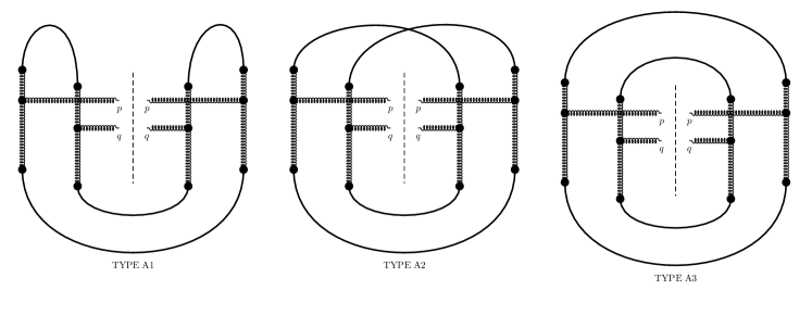
Figure 3: Type A contributions to the double inclusive gluon production
After performing the color contractions on the projectile side we get
three types of diagrams: Type A1, Type A2 and Type A3 (see
Fig. 3
Type A1 ∝ ( 2 π ) 2 δ b b ¯ δ b ¯ ′ b ′ δ ( z 1 − − ω 1 − ) δ ( z ¯ 1 − − ω ¯ 1 − ) δ ( 2 ) ( k 1 + k 2 ) δ ( 2 ) ( k 3 + k 4 ) μ P 2 ( z 1 − ) μ P 2 ( z ¯ 1 − ) proportional-to Type A1 superscript 2 𝜋 2 superscript 𝛿 𝑏 ¯ 𝑏 superscript 𝛿 superscript ¯ 𝑏 ′ superscript 𝑏 ′ 𝛿 superscript subscript 𝑧 1 superscript subscript 𝜔 1 𝛿 superscript subscript ¯ 𝑧 1 superscript subscript ¯ 𝜔 1 superscript 𝛿 2 subscript 𝑘 1 subscript 𝑘 2 superscript 𝛿 2 subscript 𝑘 3 subscript 𝑘 4 subscript superscript 𝜇 2 𝑃 superscript subscript 𝑧 1 subscript superscript 𝜇 2 𝑃 superscript subscript ¯ 𝑧 1 \displaystyle{\rm Type\,A1}\propto(2\pi)^{2}\delta^{b\bar{b}}\delta^{\bar{b}^{\prime}b^{\prime}}\delta(z_{1}^{-}-\omega_{1}^{-})\delta(\bar{z}_{1}^{-}-\bar{\omega}_{1}^{-})\delta^{(2)}(k_{1}+k_{2})\delta^{(2)}(k_{3}+k_{4})\mu^{2}_{P}(z_{1}^{-})\mu^{2}_{P}(\bar{z}_{1}^{-})\; (36)
Type A2 ∝ ( 2 π ) 2 δ b b ¯ ′ δ b ¯ b ′ δ ( z 1 − − ω ¯ 1 − ) δ ( z ¯ 1 − − ω 1 − ) δ ( 2 ) ( k 1 − k 3 ) δ ( 2 ) ( k 2 − k 4 ) μ P 2 ( z 1 − ) μ P 2 ( z ¯ 1 − ) proportional-to Type A2 superscript 2 𝜋 2 superscript 𝛿 𝑏 superscript ¯ 𝑏 ′ superscript 𝛿 ¯ 𝑏 superscript 𝑏 ′ 𝛿 superscript subscript 𝑧 1 superscript subscript ¯ 𝜔 1 𝛿 superscript subscript ¯ 𝑧 1 superscript subscript 𝜔 1 superscript 𝛿 2 subscript 𝑘 1 subscript 𝑘 3 superscript 𝛿 2 subscript 𝑘 2 subscript 𝑘 4 subscript superscript 𝜇 2 𝑃 superscript subscript 𝑧 1 subscript superscript 𝜇 2 𝑃 superscript subscript ¯ 𝑧 1 \displaystyle{\rm Type\,A2}\propto(2\pi)^{2}\delta^{b\bar{b}^{\prime}}\delta^{\bar{b}b^{\prime}}\delta(z_{1}^{-}-\bar{\omega}_{1}^{-})\delta(\bar{z}_{1}^{-}-\omega_{1}^{-})\delta^{(2)}(k_{1}-k_{3})\delta^{(2)}(k_{2}-k_{4})\mu^{2}_{P}(z_{1}^{-})\mu^{2}_{P}(\bar{z}_{1}^{-})\; (37)
Type A3 ∝ ( 2 π ) 2 δ b b ′ δ b ¯ b ¯ ′ δ ( z 1 − − z ¯ 1 − ) δ ( ω 1 − − ω ¯ 1 − ) δ ( 2 ) ( k 1 − k 4 ) δ ( 2 ) ( k 2 − k 3 ) μ P 2 ( z 1 − ) μ P 2 ( ω ¯ 1 − ) . proportional-to Type A3 superscript 2 𝜋 2 superscript 𝛿 𝑏 superscript 𝑏 ′ superscript 𝛿 ¯ 𝑏 superscript ¯ 𝑏 ′ 𝛿 superscript subscript 𝑧 1 superscript subscript ¯ 𝑧 1 𝛿 superscript subscript 𝜔 1 superscript subscript ¯ 𝜔 1 superscript 𝛿 2 subscript 𝑘 1 subscript 𝑘 4 superscript 𝛿 2 subscript 𝑘 2 subscript 𝑘 3 subscript superscript 𝜇 2 𝑃 superscript subscript 𝑧 1 subscript superscript 𝜇 2 𝑃 superscript subscript ¯ 𝜔 1 \displaystyle{\rm Type\,A3}\propto(2\pi)^{2}\delta^{bb^{\prime}}\delta^{\bar{b}\bar{b}^{\prime}}\delta(z_{1}^{-}-\bar{z}_{1}^{-})\delta(\omega_{1}^{-}-\bar{\omega}_{1}^{-})\delta^{(2)}(k_{1}-k_{4})\delta^{(2)}(k_{2}-k_{3})\mu^{2}_{P}(z_{1}^{-})\mu^{2}_{P}(\bar{\omega}_{1}^{-})\;. (38)
Using eqs. (35 38
Type A1 = f a b c f a ¯ b c ¯ f a ¯ b ¯ c ¯ f a b ¯ c S ⟂ g 8 ∫ d 2 k 1 ( 2 π ) 2 d 2 k 3 ( 2 π ) 2 δ ( 2 ) ( k 1 + k 3 ) Φ P ( k 1 2 ) Φ P ( k 3 2 ) ∫ 𝑑 z 2 + 𝑑 ω 2 + μ T 2 ( z 2 + ) μ T 2 ( ω 2 + ) Type A1 superscript 𝑓 𝑎 𝑏 𝑐 superscript 𝑓 ¯ 𝑎 𝑏 ¯ 𝑐 superscript 𝑓 ¯ 𝑎 ¯ 𝑏 ¯ 𝑐 superscript 𝑓 𝑎 ¯ 𝑏 𝑐 subscript 𝑆 perpendicular-to superscript 𝑔 8 superscript 𝑑 2 subscript 𝑘 1 superscript 2 𝜋 2 superscript 𝑑 2 subscript 𝑘 3 superscript 2 𝜋 2 superscript 𝛿 2 subscript 𝑘 1 subscript 𝑘 3 subscript Φ 𝑃 superscript subscript 𝑘 1 2 subscript Φ 𝑃 superscript subscript 𝑘 3 2 differential-d subscript superscript 𝑧 2 differential-d subscript superscript 𝜔 2 subscript superscript 𝜇 2 𝑇 superscript subscript 𝑧 2 subscript superscript 𝜇 2 𝑇 superscript subscript 𝜔 2 \displaystyle{\rm Type\,A1}=f^{abc}f^{\bar{a}b\bar{c}}f^{\bar{a}\bar{b}\bar{c}}f^{a\bar{b}c}S_{\perp}g^{8}\int\frac{d^{2}k_{1}}{(2\pi)^{2}}\frac{d^{2}k_{3}}{(2\pi)^{2}}\delta^{(2)}(k_{1}+k_{3})\Phi_{P}(k_{1}^{2})\Phi_{P}(k_{3}^{2})\int dz^{+}_{2}d\omega^{+}_{2}\mu^{2}_{T}(z_{2}^{+})\mu^{2}_{T}(\omega_{2}^{+})
2 4 C i ( p , k 1 ) C i ( p , − k 3 ) C j ( q , − k 1 ) C j ( q , k 3 ) k 1 2 k 3 2 ( p − k 1 ) 2 ( p + k 3 ) 2 ( q + k 1 ) 2 ( q − k 3 ) 2 superscript 2 4 superscript 𝐶 𝑖 𝑝 subscript 𝑘 1 superscript 𝐶 𝑖 𝑝 subscript 𝑘 3 superscript 𝐶 𝑗 𝑞 subscript 𝑘 1 superscript 𝐶 𝑗 𝑞 subscript 𝑘 3 superscript subscript 𝑘 1 2 superscript subscript 𝑘 3 2 superscript 𝑝 subscript 𝑘 1 2 superscript 𝑝 subscript 𝑘 3 2 superscript 𝑞 subscript 𝑘 1 2 superscript 𝑞 subscript 𝑘 3 2 \displaystyle 2^{4}C^{i}(p,k_{1})C^{i}(p,-k_{3})C^{j}(q,-k_{1})C^{j}(q,k_{3})\frac{k_{1}^{2}k_{3}^{2}}{(p-k_{1})^{2}(p+k_{3})^{2}(q+k_{1})^{2}(q-k_{3})^{2}} (39)
Type A2 = f a b c f a ¯ b ¯ c ¯ f a ¯ b c ¯ f a b ¯ c S ⟂ g 8 ∫ d 2 k 1 ( 2 π ) 2 d 2 k 2 ( 2 π ) 2 δ ( 2 ) ( k 1 − k 2 ) Φ P ( k 1 2 ) Φ P ( k 2 2 ) ∫ 𝑑 z 2 + 𝑑 ω 2 + μ T 2 ( z 2 + ) μ T 2 ( ω 2 + ) Type A2 superscript 𝑓 𝑎 𝑏 𝑐 superscript 𝑓 ¯ 𝑎 ¯ 𝑏 ¯ 𝑐 superscript 𝑓 ¯ 𝑎 𝑏 ¯ 𝑐 superscript 𝑓 𝑎 ¯ 𝑏 𝑐 subscript 𝑆 perpendicular-to superscript 𝑔 8 superscript 𝑑 2 subscript 𝑘 1 superscript 2 𝜋 2 superscript 𝑑 2 subscript 𝑘 2 superscript 2 𝜋 2 superscript 𝛿 2 subscript 𝑘 1 subscript 𝑘 2 subscript Φ 𝑃 superscript subscript 𝑘 1 2 subscript Φ 𝑃 superscript subscript 𝑘 2 2 differential-d subscript superscript 𝑧 2 differential-d subscript superscript 𝜔 2 subscript superscript 𝜇 2 𝑇 superscript subscript 𝑧 2 subscript superscript 𝜇 2 𝑇 superscript subscript 𝜔 2 \displaystyle{\rm Type\,A2}=f^{abc}f^{\bar{a}\bar{b}\bar{c}}f^{\bar{a}b\bar{c}}f^{a\bar{b}c}S_{\perp}g^{8}\int\frac{d^{2}k_{1}}{(2\pi)^{2}}\frac{d^{2}k_{2}}{(2\pi)^{2}}\delta^{(2)}(k_{1}-k_{2})\Phi_{P}(k_{1}^{2})\Phi_{P}(k_{2}^{2})\int dz^{+}_{2}d\omega^{+}_{2}\mu^{2}_{T}(z_{2}^{+})\mu^{2}_{T}(\omega_{2}^{+})
2 4 C i ( p , k 1 ) C i ( p , k 1 ) C j ( q , k 2 ) C j ( q , k 2 ) k 1 2 k 2 2 ( p − k 1 ) 4 ( q − k 2 ) 4 superscript 2 4 superscript 𝐶 𝑖 𝑝 subscript 𝑘 1 superscript 𝐶 𝑖 𝑝 subscript 𝑘 1 superscript 𝐶 𝑗 𝑞 subscript 𝑘 2 superscript 𝐶 𝑗 𝑞 subscript 𝑘 2 superscript subscript 𝑘 1 2 superscript subscript 𝑘 2 2 superscript 𝑝 subscript 𝑘 1 4 superscript 𝑞 subscript 𝑘 2 4 \displaystyle 2^{4}C^{i}(p,k_{1})C^{i}(p,k_{1})C^{j}(q,k_{2})C^{j}(q,k_{2})\frac{k_{1}^{2}k_{2}^{2}}{(p-k_{1})^{4}(q-k_{2})^{4}} (40)
Type A3 = f a b c f a ¯ b ¯ c ¯ f a ¯ b ¯ c ¯ f a b c S ⟂ 2 g 8 ∫ d 2 k 1 ( 2 π ) 2 d 2 k 2 ( 2 π ) 2 Φ P ( k 1 2 ) Φ P ( k 2 2 ) ∫ 𝑑 z 2 + 𝑑 ω 2 + μ T 2 ( z 2 + ) μ T 2 ( ω 2 + ) Type A3 superscript 𝑓 𝑎 𝑏 𝑐 superscript 𝑓 ¯ 𝑎 ¯ 𝑏 ¯ 𝑐 superscript 𝑓 ¯ 𝑎 ¯ 𝑏 ¯ 𝑐 superscript 𝑓 𝑎 𝑏 𝑐 subscript superscript 𝑆 2 perpendicular-to superscript 𝑔 8 superscript 𝑑 2 subscript 𝑘 1 superscript 2 𝜋 2 superscript 𝑑 2 subscript 𝑘 2 superscript 2 𝜋 2 subscript Φ 𝑃 superscript subscript 𝑘 1 2 subscript Φ 𝑃 superscript subscript 𝑘 2 2 differential-d subscript superscript 𝑧 2 differential-d subscript superscript 𝜔 2 subscript superscript 𝜇 2 𝑇 superscript subscript 𝑧 2 subscript superscript 𝜇 2 𝑇 superscript subscript 𝜔 2 \displaystyle{\rm Type\,A3}=f^{abc}f^{\bar{a}\bar{b}\bar{c}}f^{\bar{a}\bar{b}\bar{c}}f^{abc}S^{2}_{\perp}g^{8}\int\frac{d^{2}k_{1}}{(2\pi)^{2}}\frac{d^{2}k_{2}}{(2\pi)^{2}}\Phi_{P}(k_{1}^{2})\Phi_{P}(k_{2}^{2})\int dz^{+}_{2}d\omega^{+}_{2}\mu^{2}_{T}(z_{2}^{+})\mu^{2}_{T}(\omega_{2}^{+})
2 4 C i ( p , k 1 ) C i ( p , k 1 ) C j ( q , k 2 ) C j ( q , k 2 ) k 1 2 k 2 2 ( p − k 1 ) 4 ( q − k 2 ) 4 superscript 2 4 superscript 𝐶 𝑖 𝑝 subscript 𝑘 1 superscript 𝐶 𝑖 𝑝 subscript 𝑘 1 superscript 𝐶 𝑗 𝑞 subscript 𝑘 2 superscript 𝐶 𝑗 𝑞 subscript 𝑘 2 superscript subscript 𝑘 1 2 superscript subscript 𝑘 2 2 superscript 𝑝 subscript 𝑘 1 4 superscript 𝑞 subscript 𝑘 2 4 \displaystyle 2^{4}C^{i}(p,k_{1})C^{i}(p,k_{1})C^{j}(q,k_{2})C^{j}(q,k_{2})\frac{k_{1}^{2}k_{2}^{2}}{(p-k_{1})^{4}(q-k_{2})^{4}} (41)
Note that we have used eq. (14 6
Type A1 Type A1 \displaystyle{\rm Type\,A1} = \displaystyle= 16 N c 2 ( N c 2 − 1 ) g 4 S ⟂ p 2 q 2 ∫ d 2 k 1 ( 2 π ) 2 d 2 k 2 ( 2 π ) 2 δ ( 2 ) ( k 1 + k 2 ) Φ P ( k 1 2 ) Φ T [ ( p − k 1 ) 2 ] Φ P ( k 2 2 ) Φ T [ ( q − k 2 ) 2 ] 16 superscript subscript 𝑁 𝑐 2 superscript subscript 𝑁 𝑐 2 1 superscript 𝑔 4 subscript 𝑆 perpendicular-to superscript 𝑝 2 superscript 𝑞 2 superscript 𝑑 2 subscript 𝑘 1 superscript 2 𝜋 2 superscript 𝑑 2 subscript 𝑘 2 superscript 2 𝜋 2 superscript 𝛿 2 subscript 𝑘 1 subscript 𝑘 2 subscript Φ 𝑃 superscript subscript 𝑘 1 2 subscript Φ 𝑇 delimited-[] superscript 𝑝 subscript 𝑘 1 2 subscript Φ 𝑃 superscript subscript 𝑘 2 2 subscript Φ 𝑇 delimited-[] superscript 𝑞 subscript 𝑘 2 2 \displaystyle 16N_{c}^{2}(N_{c}^{2}-1)\,g^{4}\frac{S_{\perp}}{p^{2}q^{2}}\int\frac{d^{2}k_{1}}{(2\pi)^{2}}\frac{d^{2}k_{2}}{(2\pi)^{2}}\delta^{(2)}(k_{1}+k_{2})\Phi_{P}(k_{1}^{2})\Phi_{T}\big{[}(p-k_{1})^{2}\big{]}\Phi_{P}(k_{2}^{2})\Phi_{T}\big{[}(q-k_{2})^{2}\big{]} (42)
Type A2 Type A2 \displaystyle{\rm Type\,A2} = \displaystyle= 16 N c 2 ( N c 2 − 1 ) g 4 S ⟂ p 2 q 2 ∫ d 2 k 1 ( 2 π ) 2 d 2 k 2 ( 2 π ) 2 δ ( 2 ) ( k 1 − k 2 ) Φ P ( k 1 2 ) Φ T [ ( p − k 1 ) 2 ] Φ P ( k 2 2 ) Φ T [ ( q − k 2 ) 2 ] 16 superscript subscript 𝑁 𝑐 2 superscript subscript 𝑁 𝑐 2 1 superscript 𝑔 4 subscript 𝑆 perpendicular-to superscript 𝑝 2 superscript 𝑞 2 superscript 𝑑 2 subscript 𝑘 1 superscript 2 𝜋 2 superscript 𝑑 2 subscript 𝑘 2 superscript 2 𝜋 2 superscript 𝛿 2 subscript 𝑘 1 subscript 𝑘 2 subscript Φ 𝑃 superscript subscript 𝑘 1 2 subscript Φ 𝑇 delimited-[] superscript 𝑝 subscript 𝑘 1 2 subscript Φ 𝑃 superscript subscript 𝑘 2 2 subscript Φ 𝑇 delimited-[] superscript 𝑞 subscript 𝑘 2 2 \displaystyle 16N_{c}^{2}(N_{c}^{2}-1)\,g^{4}\frac{S_{\perp}}{p^{2}q^{2}}\int\frac{d^{2}k_{1}}{(2\pi)^{2}}\frac{d^{2}k_{2}}{(2\pi)^{2}}\delta^{(2)}(k_{1}-k_{2})\Phi_{P}(k_{1}^{2})\Phi_{T}\big{[}(p-k_{1})^{2}\big{]}\Phi_{P}(k_{2}^{2})\Phi_{T}\big{[}(q-k_{2})^{2}\big{]} (43)
Type A3 Type A3 \displaystyle{\rm Type\,A3} = \displaystyle= 16 N c 2 ( N c 2 − 1 ) 2 g 4 S ⟂ 2 p 2 q 2 ∫ d 2 k 1 ( 2 π ) 2 d 2 k 2 ( 2 π ) 2 Φ P ( k 1 2 ) Φ T [ ( p − k 1 ) 2 ] Φ P ( k 2 2 ) Φ T [ ( q − k 2 ) 2 ] . 16 superscript subscript 𝑁 𝑐 2 superscript superscript subscript 𝑁 𝑐 2 1 2 superscript 𝑔 4 subscript superscript 𝑆 2 perpendicular-to superscript 𝑝 2 superscript 𝑞 2 superscript 𝑑 2 subscript 𝑘 1 superscript 2 𝜋 2 superscript 𝑑 2 subscript 𝑘 2 superscript 2 𝜋 2 subscript Φ 𝑃 superscript subscript 𝑘 1 2 subscript Φ 𝑇 delimited-[] superscript 𝑝 subscript 𝑘 1 2 subscript Φ 𝑃 superscript subscript 𝑘 2 2 subscript Φ 𝑇 delimited-[] superscript 𝑞 subscript 𝑘 2 2 \displaystyle 16N_{c}^{2}(N_{c}^{2}-1)^{2}\,g^{4}\frac{S^{2}_{\perp}}{p^{2}q^{2}}\int\frac{d^{2}k_{1}}{(2\pi)^{2}}\frac{d^{2}k_{2}}{(2\pi)^{2}}\Phi_{P}(k_{1}^{2})\Phi_{T}\big{[}(p-k_{1})^{2}\big{]}\Phi_{P}(k_{2}^{2})\Phi_{T}\big{[}(q-k_{2})^{2}\big{]}~{}. (44)
As already mentioned above subeikonal corrections vanish for these diagrams.
The last expression, eq. (44
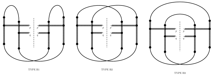
Figure 4: Type B contributions to the double inclusive gluon production
Type B contributions correspond to the following color contraction on
the target side:
⟨ ρ c ( z 2 + , p − k 1 ) ρ c ¯ ( ω 2 + , q − k 2 ) ρ ∗ c ¯ ′ ( ω ¯ 2 + , q − k 3 ) ρ ∗ c ′ ( z ¯ 2 + , p − k 4 ) ⟩ T subscript delimited-⟨⟩ superscript 𝜌 𝑐 subscript superscript 𝑧 2 𝑝 subscript 𝑘 1 superscript 𝜌 ¯ 𝑐 subscript superscript 𝜔 2 𝑞 subscript 𝑘 2 superscript 𝜌 absent superscript ¯ 𝑐 ′ subscript superscript ¯ 𝜔 2 𝑞 subscript 𝑘 3 superscript 𝜌 absent superscript 𝑐 ′ subscript superscript ¯ 𝑧 2 𝑝 subscript 𝑘 4 𝑇 \displaystyle\left\langle\rho^{c}(z^{+}_{2},p-k_{1})\rho^{\bar{c}}(\omega^{+}_{2},q-k_{2})\rho^{*\bar{c}^{\prime}}(\bar{\omega}^{+}_{2},q-k_{3})\rho^{*c^{\prime}}(\bar{z}^{+}_{2},p-k_{4})\right\rangle_{T} → → \displaystyle\to ⟨ ρ c ( z 2 + , p − k 1 ) ρ ∗ c ¯ ′ ( ω ¯ 2 + , q − k 3 ) ⟩ T subscript delimited-⟨⟩ superscript 𝜌 𝑐 subscript superscript 𝑧 2 𝑝 subscript 𝑘 1 superscript 𝜌 absent superscript ¯ 𝑐 ′ subscript superscript ¯ 𝜔 2 𝑞 subscript 𝑘 3 𝑇 \displaystyle\left\langle\rho^{c}(z^{+}_{2},p-k_{1})\rho^{*\bar{c}^{\prime}}(\bar{\omega}^{+}_{2},q-k_{3})\right\rangle_{T} (45)
× ⟨ ρ c ¯ ( ω 2 + , q − k 2 ) ρ ∗ c ′ ( z ¯ 2 + , p − k 4 ) ⟩ T . absent subscript delimited-⟨⟩ superscript 𝜌 ¯ 𝑐 subscript superscript 𝜔 2 𝑞 subscript 𝑘 2 superscript 𝜌 absent superscript 𝑐 ′ subscript superscript ¯ 𝑧 2 𝑝 subscript 𝑘 4 𝑇 \displaystyle\times\left\langle\rho^{\bar{c}}(\omega^{+}_{2},q-k_{2})\rho^{*c^{\prime}}(\bar{z}^{+}_{2},p-k_{4})\right\rangle_{T}\;.
Again, by using eq. (10
( 2 π ) 4 δ c c ¯ ′ δ c ¯ c ′ δ ( z 2 + − ω ¯ 2 + ) δ ( ω 2 + − z ¯ 2 + ) δ ( 2 ) ( p − q + k 3 − k 1 ) δ ( 2 ) ( q − p + k 4 − k 2 ) μ T 2 ( z 2 + ) μ T 2 ( ω 2 + ) . superscript 2 𝜋 4 superscript 𝛿 𝑐 superscript ¯ 𝑐 ′ superscript 𝛿 ¯ 𝑐 superscript 𝑐 ′ 𝛿 superscript subscript 𝑧 2 superscript subscript ¯ 𝜔 2 𝛿 superscript subscript 𝜔 2 superscript subscript ¯ 𝑧 2 superscript 𝛿 2 𝑝 𝑞 subscript 𝑘 3 subscript 𝑘 1 superscript 𝛿 2 𝑞 𝑝 subscript 𝑘 4 subscript 𝑘 2 subscript superscript 𝜇 2 𝑇 superscript subscript 𝑧 2 subscript superscript 𝜇 2 𝑇 superscript subscript 𝜔 2 (2\pi)^{4}\delta^{c\bar{c}^{\prime}}\delta^{\bar{c}c^{\prime}}\delta(z_{2}^{+}-\bar{\omega}_{2}^{+})\delta(\omega_{2}^{+}-\bar{z}_{2}^{+})\delta^{(2)}(p-q+k_{3}-k_{1})\delta^{(2)}(q-p+k_{4}-k_{2})\mu^{2}_{T}(z_{2}^{+})\mu^{2}_{T}(\omega_{2}^{+})\;. (46)
The color contractions on the projectile side are the same as Type A
diagrams. Hence, one can immediately write the Type B contributions to
the double inclusive gluon production cross section as
Type B1 Type B1 \displaystyle{\rm Type\;B1} = \displaystyle= f a b c f a ¯ b c ¯ f a ¯ b ¯ c f a b ¯ c ¯ S ⟂ g 8 ∫ d 2 k 1 ( 2 π ) 2 d 2 k 3 ( 2 π ) 2 δ ( 2 ) ( p − q − k 1 + k 3 ) Φ P ( k 1 2 ) Φ P ( k 3 2 ) ∫ 𝑑 z 2 + 𝑑 z ¯ 2 + μ T 2 ( z 2 + ) μ T 2 ( z ¯ 2 + ) 2 4 superscript 𝑓 𝑎 𝑏 𝑐 superscript 𝑓 ¯ 𝑎 𝑏 ¯ 𝑐 superscript 𝑓 ¯ 𝑎 ¯ 𝑏 𝑐 superscript 𝑓 𝑎 ¯ 𝑏 ¯ 𝑐 subscript 𝑆 perpendicular-to superscript 𝑔 8 superscript 𝑑 2 subscript 𝑘 1 superscript 2 𝜋 2 superscript 𝑑 2 subscript 𝑘 3 superscript 2 𝜋 2 superscript 𝛿 2 𝑝 𝑞 subscript 𝑘 1 subscript 𝑘 3 subscript Φ 𝑃 superscript subscript 𝑘 1 2 subscript Φ 𝑃 superscript subscript 𝑘 3 2 differential-d subscript superscript 𝑧 2 differential-d subscript superscript ¯ 𝑧 2 subscript superscript 𝜇 2 𝑇 superscript subscript 𝑧 2 subscript superscript 𝜇 2 𝑇 superscript subscript ¯ 𝑧 2 superscript 2 4 \displaystyle f^{abc}f^{\bar{a}b\bar{c}}f^{\bar{a}\bar{b}c}f^{a\bar{b}\bar{c}}S_{\perp}g^{8}\int\frac{d^{2}k_{1}}{(2\pi)^{2}}\frac{d^{2}k_{3}}{(2\pi)^{2}}\delta^{(2)}(p-q-k_{1}+k_{3})\Phi_{P}(k_{1}^{2})\Phi_{P}(k_{3}^{2})\int dz^{+}_{2}d\bar{z}^{+}_{2}\mu^{2}_{T}(z_{2}^{+})\mu^{2}_{T}(\bar{z}_{2}^{+})2^{4} (47)
C i ( p , k 1 ) C i ( p , − k 3 ) C j ( q , − k 1 ) C j ( q , k 3 ) k 1 2 k 3 2 ( p − k 1 ) 2 ( p + k 3 ) 2 ( q + k 1 ) 2 ( q − k 3 ) 2 { 1 − 1 8 ( p 2 p + − q 2 q + ) 2 ( z 2 + − z ¯ 2 + ) 2 } superscript 𝐶 𝑖 𝑝 subscript 𝑘 1 superscript 𝐶 𝑖 𝑝 subscript 𝑘 3 superscript 𝐶 𝑗 𝑞 subscript 𝑘 1 superscript 𝐶 𝑗 𝑞 subscript 𝑘 3 superscript subscript 𝑘 1 2 superscript subscript 𝑘 3 2 superscript 𝑝 subscript 𝑘 1 2 superscript 𝑝 subscript 𝑘 3 2 superscript 𝑞 subscript 𝑘 1 2 superscript 𝑞 subscript 𝑘 3 2 1 1 8 superscript superscript 𝑝 2 superscript 𝑝 superscript 𝑞 2 superscript 𝑞 2 superscript subscript superscript 𝑧 2 superscript subscript ¯ 𝑧 2 2 \displaystyle C^{i}(p,k_{1})C^{i}(p,-k_{3})C^{j}(q,-k_{1})C^{j}(q,k_{3})\frac{k_{1}^{2}k_{3}^{2}}{(p-k_{1})^{2}(p+k_{3})^{2}(q+k_{1})^{2}(q-k_{3})^{2}}\left\{1-\frac{1}{8}\left(\frac{p^{2}}{p^{+}}-\frac{q^{2}}{q^{+}}\right)^{2}(z^{+}_{2}-\bar{z}_{2}^{+})^{2}\right\}
= \displaystyle= 2 N c 2 ( N c 2 − 1 ) g 4 S ⟂ p 2 q 2 ∫ d 2 k 1 ( 2 π ) 2 d 2 k 2 ( 2 π ) 2 δ ( 2 ) ( p − q − k 1 + k 2 ) Φ P ( k 1 2 ) Φ T [ ( p − k 1 ) 2 ] Φ P ( k 2 2 ) Φ T [ ( q − k 2 ) 2 ] 2 superscript subscript 𝑁 𝑐 2 superscript subscript 𝑁 𝑐 2 1 superscript 𝑔 4 subscript 𝑆 perpendicular-to superscript 𝑝 2 superscript 𝑞 2 superscript 𝑑 2 subscript 𝑘 1 superscript 2 𝜋 2 superscript 𝑑 2 subscript 𝑘 2 superscript 2 𝜋 2 superscript 𝛿 2 𝑝 𝑞 subscript 𝑘 1 subscript 𝑘 2 subscript Φ 𝑃 superscript subscript 𝑘 1 2 subscript Φ 𝑇 delimited-[] superscript 𝑝 subscript 𝑘 1 2 subscript Φ 𝑃 superscript subscript 𝑘 2 2 subscript Φ 𝑇 delimited-[] superscript 𝑞 subscript 𝑘 2 2 \displaystyle 2N_{c}^{2}(N_{c}^{2}-1)g^{4}\frac{S_{\perp}}{p^{2}q^{2}}\int\frac{d^{2}k_{1}}{(2\pi)^{2}}\frac{d^{2}k_{2}}{(2\pi)^{2}}\delta^{(2)}(p-q-k_{1}+k_{2})\Phi_{P}(k_{1}^{2})\Phi_{T}\big{[}(p-k_{1})^{2}\big{]}\Phi_{P}(k_{2}^{2})\Phi_{T}\big{[}(q-k_{2})^{2}\big{]}
× { 1 + k 2 2 ( p − k 1 ) 2 k 1 2 ( p + k 2 ) 2 − p 2 ( k 1 + k 2 ) 2 k 1 2 ( p + k 2 ) 2 } { 1 + k 1 2 ( q − k 2 ) 2 k 2 2 ( q + k 1 ) 2 − q 2 ( k 1 + k 2 ) 2 k 2 2 ( q + k 1 ) 2 } [ 1 − 1 12 ( p 2 2 p + − q 2 2 q + ) 2 ℓ + 2 ] absent 1 superscript subscript 𝑘 2 2 superscript 𝑝 subscript 𝑘 1 2 superscript subscript 𝑘 1 2 superscript 𝑝 subscript 𝑘 2 2 superscript 𝑝 2 superscript subscript 𝑘 1 subscript 𝑘 2 2 superscript subscript 𝑘 1 2 superscript 𝑝 subscript 𝑘 2 2 1 superscript subscript 𝑘 1 2 superscript 𝑞 subscript 𝑘 2 2 superscript subscript 𝑘 2 2 superscript 𝑞 subscript 𝑘 1 2 superscript 𝑞 2 superscript subscript 𝑘 1 subscript 𝑘 2 2 superscript subscript 𝑘 2 2 superscript 𝑞 subscript 𝑘 1 2 delimited-[] 1 1 12 superscript superscript 𝑝 2 2 superscript 𝑝 superscript 𝑞 2 2 superscript 𝑞 2 superscript superscript ℓ 2 \displaystyle\times\left\{1+\frac{k_{2}^{2}(p-k_{1})^{2}}{k_{1}^{2}(p+k_{2})^{2}}-\frac{p^{2}(k_{1}+k_{2})^{2}}{k_{1}^{2}(p+k_{2})^{2}}\right\}\left\{1+\frac{k_{1}^{2}(q-k_{2})^{2}}{k_{2}^{2}(q+k_{1})^{2}}-\frac{q^{2}(k_{1}+k_{2})^{2}}{k_{2}^{2}(q+k_{1})^{2}}\right\}\left[1-\frac{1}{12}\left(\frac{p^{2}}{2p^{+}}-\frac{q^{2}}{2q^{+}}\right)^{2}{\ell^{+}}^{2}\right]
Type B2 Type B2 \displaystyle{\rm Type\;B2} = \displaystyle= f a b c f a ¯ b ¯ c ¯ f a ¯ b c f a b ¯ c ¯ S ⟂ g 8 δ ( 2 ) ( p − q ) ∫ d 2 k 1 ( 2 π ) 2 d 2 k 2 ( 2 π ) 2 Φ P ( k 1 2 ) Φ P ( k 2 2 ) ∫ 𝑑 z 2 + 𝑑 z ¯ 2 + μ T 2 ( z 2 + ) μ T 2 ( z ¯ 2 + ) 2 4 superscript 𝑓 𝑎 𝑏 𝑐 superscript 𝑓 ¯ 𝑎 ¯ 𝑏 ¯ 𝑐 superscript 𝑓 ¯ 𝑎 𝑏 𝑐 superscript 𝑓 𝑎 ¯ 𝑏 ¯ 𝑐 subscript 𝑆 perpendicular-to superscript 𝑔 8 superscript 𝛿 2 𝑝 𝑞 superscript 𝑑 2 subscript 𝑘 1 superscript 2 𝜋 2 superscript 𝑑 2 subscript 𝑘 2 superscript 2 𝜋 2 subscript Φ 𝑃 superscript subscript 𝑘 1 2 subscript Φ 𝑃 superscript subscript 𝑘 2 2 differential-d subscript superscript 𝑧 2 differential-d subscript superscript ¯ 𝑧 2 subscript superscript 𝜇 2 𝑇 superscript subscript 𝑧 2 subscript superscript 𝜇 2 𝑇 superscript subscript ¯ 𝑧 2 superscript 2 4 \displaystyle f^{abc}f^{\bar{a}\bar{b}\bar{c}}f^{\bar{a}bc}f^{a\bar{b}\bar{c}}S_{\perp}g^{8}\delta^{(2)}(p-q)\int\frac{d^{2}k_{1}}{(2\pi)^{2}}\frac{d^{2}k_{2}}{(2\pi)^{2}}\Phi_{P}(k_{1}^{2})\Phi_{P}(k_{2}^{2})\int dz^{+}_{2}d\bar{z}^{+}_{2}\mu^{2}_{T}(z_{2}^{+})\mu^{2}_{T}(\bar{z}_{2}^{+})2^{4} (48)
C i ( p , k 1 ) C i ( p , k 2 ) C j ( q , k 1 ) C j ( q , k 2 ) k 1 2 k 2 2 ( p − k 1 ) 2 ( p − k 2 ) 2 ( q − k 1 ) 2 ( q − k 2 ) 2 { 1 − 1 8 ( p 2 p + − q 2 q + ) 2 ( z 2 + − z ¯ 2 + ) 2 } superscript 𝐶 𝑖 𝑝 subscript 𝑘 1 superscript 𝐶 𝑖 𝑝 subscript 𝑘 2 superscript 𝐶 𝑗 𝑞 subscript 𝑘 1 superscript 𝐶 𝑗 𝑞 subscript 𝑘 2 superscript subscript 𝑘 1 2 superscript subscript 𝑘 2 2 superscript 𝑝 subscript 𝑘 1 2 superscript 𝑝 subscript 𝑘 2 2 superscript 𝑞 subscript 𝑘 1 2 superscript 𝑞 subscript 𝑘 2 2 1 1 8 superscript superscript 𝑝 2 superscript 𝑝 superscript 𝑞 2 superscript 𝑞 2 superscript subscript superscript 𝑧 2 superscript subscript ¯ 𝑧 2 2 \displaystyle C^{i}(p,k_{1})C^{i}(p,k_{2})C^{j}(q,k_{1})C^{j}(q,k_{2})\frac{k_{1}^{2}k_{2}^{2}}{(p-k_{1})^{2}(p-k_{2})^{2}(q-k_{1})^{2}(q-k_{2})^{2}}\left\{1-\frac{1}{8}\left(\frac{p^{2}}{p^{+}}-\frac{q^{2}}{q^{+}}\right)^{2}(z^{+}_{2}-\bar{z}_{2}^{+})^{2}\right\}
= \displaystyle= 4 N c 2 ( N c 2 − 1 ) g 4 S ⟂ p 2 q 2 δ ( 2 ) ( p − q ) ∫ d 2 k 1 ( 2 π ) 2 d 2 k 2 ( 2 π ) 2 Φ P ( k 1 2 ) Φ T [ ( p − k 1 ) 2 ] Φ P ( k 2 2 ) Φ T [ ( q − k 2 ) 2 ] 4 superscript subscript 𝑁 𝑐 2 superscript subscript 𝑁 𝑐 2 1 superscript 𝑔 4 subscript 𝑆 perpendicular-to superscript 𝑝 2 superscript 𝑞 2 superscript 𝛿 2 𝑝 𝑞 superscript 𝑑 2 subscript 𝑘 1 superscript 2 𝜋 2 superscript 𝑑 2 subscript 𝑘 2 superscript 2 𝜋 2 subscript Φ 𝑃 superscript subscript 𝑘 1 2 subscript Φ 𝑇 delimited-[] superscript 𝑝 subscript 𝑘 1 2 subscript Φ 𝑃 superscript subscript 𝑘 2 2 subscript Φ 𝑇 delimited-[] superscript 𝑞 subscript 𝑘 2 2 \displaystyle 4N_{c}^{2}(N_{c}^{2}-1)g^{4}\frac{S_{\perp}}{p^{2}q^{2}}\delta^{(2)}(p-q)\int\frac{d^{2}k_{1}}{(2\pi)^{2}}\frac{d^{2}k_{2}}{(2\pi)^{2}}\Phi_{P}(k_{1}^{2})\Phi_{T}\big{[}(p-k_{1})^{2}\big{]}\Phi_{P}(k_{2}^{2})\Phi_{T}\big{[}(q-k_{2})^{2}\big{]}
× { 1 + k 2 2 ( p − k 1 ) 2 k 1 2 ( p − k 2 ) 2 − p 2 ( k 1 − k 2 ) 2 k 1 2 ( p − k 2 ) 2 } { 1 + k 1 2 ( q − k 2 ) 2 k 2 2 ( q − k 1 ) 2 − q 2 ( k 1 − k 2 ) 2 k 2 2 ( q − k 1 ) 2 } [ 1 − 1 12 ( p 2 2 p + − q 2 2 q + ) 2 ℓ + 2 ] absent 1 superscript subscript 𝑘 2 2 superscript 𝑝 subscript 𝑘 1 2 superscript subscript 𝑘 1 2 superscript 𝑝 subscript 𝑘 2 2 superscript 𝑝 2 superscript subscript 𝑘 1 subscript 𝑘 2 2 superscript subscript 𝑘 1 2 superscript 𝑝 subscript 𝑘 2 2 1 superscript subscript 𝑘 1 2 superscript 𝑞 subscript 𝑘 2 2 superscript subscript 𝑘 2 2 superscript 𝑞 subscript 𝑘 1 2 superscript 𝑞 2 superscript subscript 𝑘 1 subscript 𝑘 2 2 superscript subscript 𝑘 2 2 superscript 𝑞 subscript 𝑘 1 2 delimited-[] 1 1 12 superscript superscript 𝑝 2 2 superscript 𝑝 superscript 𝑞 2 2 superscript 𝑞 2 superscript superscript ℓ 2 \displaystyle\times\left\{1+\frac{k_{2}^{2}(p-k_{1})^{2}}{k_{1}^{2}(p-k_{2})^{2}}-\frac{p^{2}(k_{1}-k_{2})^{2}}{k_{1}^{2}(p-k_{2})^{2}}\right\}\left\{1+\frac{k_{1}^{2}(q-k_{2})^{2}}{k_{2}^{2}(q-k_{1})^{2}}-\frac{q^{2}(k_{1}-k_{2})^{2}}{k_{2}^{2}(q-k_{1})^{2}}\right\}\left[1-\frac{1}{12}\left(\frac{p^{2}}{2p^{+}}-\frac{q^{2}}{2q^{+}}\right)^{2}{\ell^{+}}^{2}\right]
Type B3 Type B3 \displaystyle{\rm Type\;B3} = \displaystyle= f a b c f a ¯ b ¯ c ¯ f a ¯ b ¯ c f a b c ¯ S ⟂ g 8 ∫ d 2 k 1 ( 2 π ) 2 d 2 k 2 ( 2 π ) 2 δ ( 2 ) ( p − q − k 1 + k 2 ) Φ P ( k 1 2 ) Φ P ( k 2 2 ) ∫ 𝑑 z 2 + 𝑑 z ¯ 2 + μ T 2 ( z 2 + ) μ T 2 ( z ¯ 2 + ) 2 4 superscript 𝑓 𝑎 𝑏 𝑐 superscript 𝑓 ¯ 𝑎 ¯ 𝑏 ¯ 𝑐 superscript 𝑓 ¯ 𝑎 ¯ 𝑏 𝑐 superscript 𝑓 𝑎 𝑏 ¯ 𝑐 subscript 𝑆 perpendicular-to superscript 𝑔 8 superscript 𝑑 2 subscript 𝑘 1 superscript 2 𝜋 2 superscript 𝑑 2 subscript 𝑘 2 superscript 2 𝜋 2 superscript 𝛿 2 𝑝 𝑞 subscript 𝑘 1 subscript 𝑘 2 subscript Φ 𝑃 superscript subscript 𝑘 1 2 subscript Φ 𝑃 superscript subscript 𝑘 2 2 differential-d subscript superscript 𝑧 2 differential-d subscript superscript ¯ 𝑧 2 subscript superscript 𝜇 2 𝑇 superscript subscript 𝑧 2 subscript superscript 𝜇 2 𝑇 superscript subscript ¯ 𝑧 2 superscript 2 4 \displaystyle f^{abc}f^{\bar{a}\bar{b}\bar{c}}f^{\bar{a}\bar{b}c}f^{ab\bar{c}}S_{\perp}g^{8}\int\frac{d^{2}k_{1}}{(2\pi)^{2}}\frac{d^{2}k_{2}}{(2\pi)^{2}}\delta^{(2)}(p-q-k_{1}+k_{2})\Phi_{P}(k_{1}^{2})\Phi_{P}(k_{2}^{2})\int dz^{+}_{2}d\bar{z}^{+}_{2}\mu^{2}_{T}(z_{2}^{+})\mu^{2}_{T}(\bar{z}_{2}^{+})2^{4} (49)
C i ( p , k 1 ) C i ( p , k 1 ) C j ( q , k 2 ) C j ( q , k 2 ) k 1 2 k 2 2 ( p − k 1 ) 4 ( q − k 2 ) 4 { 1 − 1 8 ( p 2 p + − q 2 q + ) 2 ( z 2 + − z ¯ 2 + ) 2 } superscript 𝐶 𝑖 𝑝 subscript 𝑘 1 superscript 𝐶 𝑖 𝑝 subscript 𝑘 1 superscript 𝐶 𝑗 𝑞 subscript 𝑘 2 superscript 𝐶 𝑗 𝑞 subscript 𝑘 2 superscript subscript 𝑘 1 2 superscript subscript 𝑘 2 2 superscript 𝑝 subscript 𝑘 1 4 superscript 𝑞 subscript 𝑘 2 4 1 1 8 superscript superscript 𝑝 2 superscript 𝑝 superscript 𝑞 2 superscript 𝑞 2 superscript subscript superscript 𝑧 2 superscript subscript ¯ 𝑧 2 2 \displaystyle C^{i}(p,k_{1})C^{i}(p,k_{1})C^{j}(q,k_{2})C^{j}(q,k_{2})\frac{k_{1}^{2}k_{2}^{2}}{(p-k_{1})^{4}(q-k_{2})^{4}}\left\{1-\frac{1}{8}\left(\frac{p^{2}}{p^{+}}-\frac{q^{2}}{q^{+}}\right)^{2}(z^{+}_{2}-\bar{z}_{2}^{+})^{2}\right\}
= \displaystyle= 16 N c 2 ( N c 2 − 1 ) g 4 S ⟂ p 2 q 2 ∫ d 2 k 1 ( 2 π ) 2 d 2 k 2 ( 2 π ) 2 δ ( 2 ) ( p − q − k 1 + k 2 ) Φ P ( k 1 2 ) Φ T [ ( p − k 1 ) 2 ] Φ P ( k 2 2 ) Φ T [ ( q − k 2 ) 2 ] 16 superscript subscript 𝑁 𝑐 2 superscript subscript 𝑁 𝑐 2 1 superscript 𝑔 4 subscript 𝑆 perpendicular-to superscript 𝑝 2 superscript 𝑞 2 superscript 𝑑 2 subscript 𝑘 1 superscript 2 𝜋 2 superscript 𝑑 2 subscript 𝑘 2 superscript 2 𝜋 2 superscript 𝛿 2 𝑝 𝑞 subscript 𝑘 1 subscript 𝑘 2 subscript Φ 𝑃 superscript subscript 𝑘 1 2 subscript Φ 𝑇 delimited-[] superscript 𝑝 subscript 𝑘 1 2 subscript Φ 𝑃 superscript subscript 𝑘 2 2 subscript Φ 𝑇 delimited-[] superscript 𝑞 subscript 𝑘 2 2 \displaystyle 16N_{c}^{2}(N_{c}^{2}-1)g^{4}\frac{S_{\perp}}{p^{2}q^{2}}\int\frac{d^{2}k_{1}}{(2\pi)^{2}}\frac{d^{2}k_{2}}{(2\pi)^{2}}\delta^{(2)}(p-q-k_{1}+k_{2})\Phi_{P}(k_{1}^{2})\Phi_{T}\big{[}(p-k_{1})^{2}\big{]}\Phi_{P}(k_{2}^{2})\Phi_{T}\big{[}(q-k_{2})^{2}\big{]}
× [ 1 − 1 12 ( p 2 2 p + − q 2 2 q + ) 2 ℓ + 2 ] absent delimited-[] 1 1 12 superscript superscript 𝑝 2 2 superscript 𝑝 superscript 𝑞 2 2 superscript 𝑞 2 superscript superscript ℓ 2 \displaystyle\times\left[1-\frac{1}{12}\left(\frac{p^{2}}{2p^{+}}-\frac{q^{2}}{2q^{+}}\right)^{2}{\ell^{+}}^{2}\right]
To perform the longitudinal integrations explicitly we have assumed
that μ T 2 subscript superscript 𝜇 2 𝑇 \mu^{2}_{T} z 2 + superscript subscript 𝑧 2 z_{2}^{+} z ¯ 2 + subscript superscript ¯ 𝑧 2 \bar{z}^{+}_{2}
C i ( p , k 1 ) C i ( p , k 2 ) superscript 𝐶 𝑖 𝑝 subscript 𝑘 1 superscript 𝐶 𝑖 𝑝 subscript 𝑘 2 \displaystyle C^{i}(p,k_{1})C^{i}(p,k_{2}) = \displaystyle= ( p i p 2 − k 1 i k 1 2 ) ( p i p 2 − k 2 i k 2 2 ) = 1 2 p 2 k 1 2 k 2 2 [ k 1 2 ( p − k 2 ) 2 + k 2 2 ( p − k 1 ) 2 − p 2 ( k 1 − k 2 ) 2 ] superscript 𝑝 𝑖 superscript 𝑝 2 superscript subscript 𝑘 1 𝑖 superscript subscript 𝑘 1 2 superscript 𝑝 𝑖 superscript 𝑝 2 superscript subscript 𝑘 2 𝑖 superscript subscript 𝑘 2 2 1 2 superscript 𝑝 2 superscript subscript 𝑘 1 2 superscript subscript 𝑘 2 2 delimited-[] superscript subscript 𝑘 1 2 superscript 𝑝 subscript 𝑘 2 2 superscript subscript 𝑘 2 2 superscript 𝑝 subscript 𝑘 1 2 superscript 𝑝 2 superscript subscript 𝑘 1 subscript 𝑘 2 2 \displaystyle\left(\frac{p^{i}}{p^{2}}-\frac{k_{1}^{i}}{k_{1}^{2}}\right)\left(\frac{p^{i}}{p^{2}}-\frac{k_{2}^{i}}{k_{2}^{2}}\right)=\frac{1}{2p^{2}k_{1}^{2}k_{2}^{2}}\left[k_{1}^{2}(p-k_{2})^{2}+k_{2}^{2}(p-k_{1})^{2}-p^{2}(k_{1}-k_{2})^{2}\right] (50)
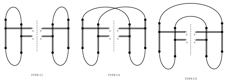
Figure 5: Type C contributions to the double inclusive gluon production
The color contractions on the target side for Type C contributions are given by
⟨ ρ c ( z 2 + , p − k 1 ) ρ c ¯ ( ω 2 + , q − k 2 ) ρ ∗ c ¯ ′ ( ω ¯ 2 + , q − k 3 ) ρ ∗ c ′ ( z ¯ 2 + , p − k 4 ) ⟩ T subscript delimited-⟨⟩ superscript 𝜌 𝑐 subscript superscript 𝑧 2 𝑝 subscript 𝑘 1 superscript 𝜌 ¯ 𝑐 subscript superscript 𝜔 2 𝑞 subscript 𝑘 2 superscript 𝜌 absent superscript ¯ 𝑐 ′ subscript superscript ¯ 𝜔 2 𝑞 subscript 𝑘 3 superscript 𝜌 absent superscript 𝑐 ′ subscript superscript ¯ 𝑧 2 𝑝 subscript 𝑘 4 𝑇 \displaystyle\left\langle\rho^{c}(z^{+}_{2},p-k_{1})\rho^{\bar{c}}(\omega^{+}_{2},q-k_{2})\rho^{*\bar{c}^{\prime}}(\bar{\omega}^{+}_{2},q-k_{3})\rho^{*c^{\prime}}(\bar{z}^{+}_{2},p-k_{4})\right\rangle_{T} → → \displaystyle\to ⟨ ρ c ( z 2 + , p − k 1 ) ρ ∗ c ¯ ( ω 2 + , q − k 2 ) ⟩ T subscript delimited-⟨⟩ superscript 𝜌 𝑐 subscript superscript 𝑧 2 𝑝 subscript 𝑘 1 superscript 𝜌 absent ¯ 𝑐 subscript superscript 𝜔 2 𝑞 subscript 𝑘 2 𝑇 \displaystyle\left\langle\rho^{c}(z^{+}_{2},p-k_{1})\rho^{*\bar{c}}(\omega^{+}_{2},q-k_{2})\right\rangle_{T} (51)
× ⟨ ρ c ¯ ′ ( ω ¯ 2 + , q − k 3 ) ρ ∗ c ′ ( z ¯ 2 + , p − k 4 ) ⟩ T . absent subscript delimited-⟨⟩ superscript 𝜌 superscript ¯ 𝑐 ′ subscript superscript ¯ 𝜔 2 𝑞 subscript 𝑘 3 superscript 𝜌 absent superscript 𝑐 ′ subscript superscript ¯ 𝑧 2 𝑝 subscript 𝑘 4 𝑇 \displaystyle\times\left\langle\rho^{\bar{c}^{\prime}}(\bar{\omega}^{+}_{2},q-k_{3})\rho^{*c^{\prime}}(\bar{z}^{+}_{2},p-k_{4})\right\rangle_{T}\;.
Thus, they are proportional to
( 2 π ) 4 δ c c ¯ δ c ¯ ′ c ′ δ ( z 2 + − ω 2 + ) δ ( z ¯ 2 + − ω ¯ 2 + ) δ ( 2 ) ( p + q − k 1 − k 2 ) δ ( 2 ) ( p + q − k 3 − k 4 ) μ T 2 ( z 2 + ) μ T 2 ( z ¯ 2 + ) . superscript 2 𝜋 4 superscript 𝛿 𝑐 ¯ 𝑐 superscript 𝛿 superscript ¯ 𝑐 ′ superscript 𝑐 ′ 𝛿 superscript subscript 𝑧 2 subscript superscript 𝜔 2 𝛿 superscript subscript ¯ 𝑧 2 superscript subscript ¯ 𝜔 2 superscript 𝛿 2 𝑝 𝑞 subscript 𝑘 1 subscript 𝑘 2 superscript 𝛿 2 𝑝 𝑞 subscript 𝑘 3 subscript 𝑘 4 subscript superscript 𝜇 2 𝑇 superscript subscript 𝑧 2 subscript superscript 𝜇 2 𝑇 superscript subscript ¯ 𝑧 2 (2\pi)^{4}\delta^{c\bar{c}}\delta^{\bar{c}^{\prime}c^{\prime}}\delta(z_{2}^{+}-\omega^{+}_{2})\delta(\bar{z}_{2}^{+}-\bar{\omega}_{2}^{+})\delta^{(2)}(p+q-k_{1}-k_{2})\delta^{(2)}(p+q-k_{3}-k_{4})\mu^{2}_{T}(z_{2}^{+})\mu^{2}_{T}(\bar{z}_{2}^{+})\;. (52)
Since the color contractions on the projectile side are the same as
Type A and Type B diagrams, one can write the Type C contributions to
the double inclusive gluon production cross section as follows:
Type C1 Type C1 \displaystyle{\rm Type\;C1} = \displaystyle= f a b c f a ¯ b c f a ¯ b ¯ c ¯ f a b ¯ c ¯ S ⟂ g 8 δ ( 2 ) ( p + q ) ∫ d 2 k 1 ( 2 π ) 2 d 2 k 3 ( 2 π ) 2 Φ P ( k 1 2 ) Φ P ( k 3 2 ) ∫ 𝑑 z 2 + 𝑑 z ¯ 2 + μ T 2 ( z 2 + ) μ T 2 ( z ¯ 2 + ) 2 4 superscript 𝑓 𝑎 𝑏 𝑐 superscript 𝑓 ¯ 𝑎 𝑏 𝑐 superscript 𝑓 ¯ 𝑎 ¯ 𝑏 ¯ 𝑐 superscript 𝑓 𝑎 ¯ 𝑏 ¯ 𝑐 subscript 𝑆 perpendicular-to superscript 𝑔 8 superscript 𝛿 2 𝑝 𝑞 superscript 𝑑 2 subscript 𝑘 1 superscript 2 𝜋 2 superscript 𝑑 2 subscript 𝑘 3 superscript 2 𝜋 2 subscript Φ 𝑃 superscript subscript 𝑘 1 2 subscript Φ 𝑃 superscript subscript 𝑘 3 2 differential-d subscript superscript 𝑧 2 differential-d subscript superscript ¯ 𝑧 2 subscript superscript 𝜇 2 𝑇 superscript subscript 𝑧 2 subscript superscript 𝜇 2 𝑇 superscript subscript ¯ 𝑧 2 superscript 2 4 \displaystyle f^{abc}f^{\bar{a}bc}f^{\bar{a}\bar{b}\bar{c}}f^{a\bar{b}\bar{c}}S_{\perp}g^{8}\delta^{(2)}(p+q)\int\frac{d^{2}k_{1}}{(2\pi)^{2}}\frac{d^{2}k_{3}}{(2\pi)^{2}}\Phi_{P}(k_{1}^{2})\Phi_{P}(k_{3}^{2})\int dz^{+}_{2}d\bar{z}^{+}_{2}\mu^{2}_{T}(z_{2}^{+})\mu^{2}_{T}(\bar{z}_{2}^{+})2^{4} (53)
C i ( p , k 1 ) C i ( p , − k 3 ) C j ( q , − k 1 ) C j ( q , k 3 ) k 1 2 k 3 2 ( p − k 1 ) 2 ( p + k 3 ) 2 ( q + k 1 ) 2 ( q − k 3 ) 2 { 1 − 1 8 ( p 2 p + + q 2 q + ) 2 ( z 2 + − z ¯ 2 + ) 2 } superscript 𝐶 𝑖 𝑝 subscript 𝑘 1 superscript 𝐶 𝑖 𝑝 subscript 𝑘 3 superscript 𝐶 𝑗 𝑞 subscript 𝑘 1 superscript 𝐶 𝑗 𝑞 subscript 𝑘 3 superscript subscript 𝑘 1 2 superscript subscript 𝑘 3 2 superscript 𝑝 subscript 𝑘 1 2 superscript 𝑝 subscript 𝑘 3 2 superscript 𝑞 subscript 𝑘 1 2 superscript 𝑞 subscript 𝑘 3 2 1 1 8 superscript superscript 𝑝 2 superscript 𝑝 superscript 𝑞 2 superscript 𝑞 2 superscript subscript superscript 𝑧 2 superscript subscript ¯ 𝑧 2 2 \displaystyle C^{i}(p,k_{1})C^{i}(p,-k_{3})C^{j}(q,-k_{1})C^{j}(q,k_{3})\frac{k_{1}^{2}k_{3}^{2}}{(p-k_{1})^{2}(p+k_{3})^{2}(q+k_{1})^{2}(q-k_{3})^{2}}\left\{1-\frac{1}{8}\left(\frac{p^{2}}{p^{+}}+\frac{q^{2}}{q^{+}}\right)^{2}(z^{+}_{2}-\bar{z}_{2}^{+})^{2}\right\}
= \displaystyle= 4 N c 2 ( N c 2 − 1 ) g 4 S ⟂ p 2 q 2 δ ( 2 ) ( p + q ) ∫ d 2 k 1 ( 2 π ) 2 d 2 k 2 ( 2 π ) 2 Φ P ( k 1 2 ) Φ T [ ( p − k 1 ) 2 ] Φ P ( k 2 2 ) Φ T [ ( q − k 2 ) 2 ] 4 superscript subscript 𝑁 𝑐 2 superscript subscript 𝑁 𝑐 2 1 superscript 𝑔 4 subscript 𝑆 perpendicular-to superscript 𝑝 2 superscript 𝑞 2 superscript 𝛿 2 𝑝 𝑞 superscript 𝑑 2 subscript 𝑘 1 superscript 2 𝜋 2 superscript 𝑑 2 subscript 𝑘 2 superscript 2 𝜋 2 subscript Φ 𝑃 superscript subscript 𝑘 1 2 subscript Φ 𝑇 delimited-[] superscript 𝑝 subscript 𝑘 1 2 subscript Φ 𝑃 superscript subscript 𝑘 2 2 subscript Φ 𝑇 delimited-[] superscript 𝑞 subscript 𝑘 2 2 \displaystyle 4N_{c}^{2}(N_{c}^{2}-1)g^{4}\frac{S_{\perp}}{p^{2}q^{2}}\delta^{(2)}(p+q)\int\frac{d^{2}k_{1}}{(2\pi)^{2}}\frac{d^{2}k_{2}}{(2\pi)^{2}}\Phi_{P}(k_{1}^{2})\Phi_{T}\big{[}(p-k_{1})^{2}\big{]}\Phi_{P}(k_{2}^{2})\Phi_{T}\big{[}(q-k_{2})^{2}\big{]}
× { 1 + k 2 2 ( p − k 1 ) 2 k 1 2 ( p + k 2 ) 2 − p 2 ( k 1 + k 2 ) 2 k 1 2 ( p + k 2 ) 2 } { 1 + k 1 2 ( q − k 2 ) 2 k 2 2 ( q + k 1 ) 2 − q 2 ( k 1 + k 2 ) 2 k 2 2 ( q + k 1 ) 2 } [ 1 − 1 12 ( p 2 2 p + + q 2 2 q + ) 2 ℓ + 2 ] absent 1 superscript subscript 𝑘 2 2 superscript 𝑝 subscript 𝑘 1 2 superscript subscript 𝑘 1 2 superscript 𝑝 subscript 𝑘 2 2 superscript 𝑝 2 superscript subscript 𝑘 1 subscript 𝑘 2 2 superscript subscript 𝑘 1 2 superscript 𝑝 subscript 𝑘 2 2 1 superscript subscript 𝑘 1 2 superscript 𝑞 subscript 𝑘 2 2 superscript subscript 𝑘 2 2 superscript 𝑞 subscript 𝑘 1 2 superscript 𝑞 2 superscript subscript 𝑘 1 subscript 𝑘 2 2 superscript subscript 𝑘 2 2 superscript 𝑞 subscript 𝑘 1 2 delimited-[] 1 1 12 superscript superscript 𝑝 2 2 superscript 𝑝 superscript 𝑞 2 2 superscript 𝑞 2 superscript superscript ℓ 2 \displaystyle\times\left\{1+\frac{k_{2}^{2}(p-k_{1})^{2}}{k_{1}^{2}(p+k_{2})^{2}}-\frac{p^{2}(k_{1}+k_{2})^{2}}{k_{1}^{2}(p+k_{2})^{2}}\right\}\left\{1+\frac{k_{1}^{2}(q-k_{2})^{2}}{k_{2}^{2}(q+k_{1})^{2}}-\frac{q^{2}(k_{1}+k_{2})^{2}}{k_{2}^{2}(q+k_{1})^{2}}\right\}\left[1-\frac{1}{12}\left(\frac{p^{2}}{2p^{+}}+\frac{q^{2}}{2q^{+}}\right)^{2}{\ell^{+}}^{2}\right]
Type C2 Type C2 \displaystyle{\rm Type\;C2} = \displaystyle= f a b c f a ¯ b ¯ c f a ¯ b c ¯ f a b ¯ c ¯ S ⟂ g 8 ∫ d 2 k 1 ( 2 π ) 2 d 2 k 2 ( 2 π ) 2 δ ( 2 ) ( p + q − k 1 − k 2 ) Φ P ( k 1 2 ) Φ P ( k 2 2 ) ∫ 𝑑 z 2 + 𝑑 z ¯ 2 + μ T 2 ( z 2 + ) μ T 2 ( z ¯ 2 + ) 2 4 superscript 𝑓 𝑎 𝑏 𝑐 superscript 𝑓 ¯ 𝑎 ¯ 𝑏 𝑐 superscript 𝑓 ¯ 𝑎 𝑏 ¯ 𝑐 superscript 𝑓 𝑎 ¯ 𝑏 ¯ 𝑐 subscript 𝑆 perpendicular-to superscript 𝑔 8 superscript 𝑑 2 subscript 𝑘 1 superscript 2 𝜋 2 superscript 𝑑 2 subscript 𝑘 2 superscript 2 𝜋 2 superscript 𝛿 2 𝑝 𝑞 subscript 𝑘 1 subscript 𝑘 2 subscript Φ 𝑃 superscript subscript 𝑘 1 2 subscript Φ 𝑃 superscript subscript 𝑘 2 2 differential-d subscript superscript 𝑧 2 differential-d subscript superscript ¯ 𝑧 2 subscript superscript 𝜇 2 𝑇 superscript subscript 𝑧 2 subscript superscript 𝜇 2 𝑇 superscript subscript ¯ 𝑧 2 superscript 2 4 \displaystyle f^{abc}f^{\bar{a}\bar{b}c}f^{\bar{a}b\bar{c}}f^{a\bar{b}\bar{c}}S_{\perp}g^{8}\int\frac{d^{2}k_{1}}{(2\pi)^{2}}\frac{d^{2}k_{2}}{(2\pi)^{2}}\delta^{(2)}(p+q-k_{1}-k_{2})\Phi_{P}(k_{1}^{2})\Phi_{P}(k_{2}^{2})\int dz^{+}_{2}d\bar{z}^{+}_{2}\mu^{2}_{T}(z_{2}^{+})\mu^{2}_{T}(\bar{z}_{2}^{+})2^{4} (54)
C i ( p , k 1 ) C i ( p , k 2 ) C j ( q , k 1 ) C j ( q , k 2 ) k 1 2 k 2 2 ( p − k 1 ) 2 ( p − k 2 ) 2 ( q − k 1 ) 2 ( q − k 2 ) 2 { 1 − 1 8 ( p 2 p + + q 2 q + ) 2 ( z 2 + − z ¯ 2 + ) 2 } superscript 𝐶 𝑖 𝑝 subscript 𝑘 1 superscript 𝐶 𝑖 𝑝 subscript 𝑘 2 superscript 𝐶 𝑗 𝑞 subscript 𝑘 1 superscript 𝐶 𝑗 𝑞 subscript 𝑘 2 superscript subscript 𝑘 1 2 superscript subscript 𝑘 2 2 superscript 𝑝 subscript 𝑘 1 2 superscript 𝑝 subscript 𝑘 2 2 superscript 𝑞 subscript 𝑘 1 2 superscript 𝑞 subscript 𝑘 2 2 1 1 8 superscript superscript 𝑝 2 superscript 𝑝 superscript 𝑞 2 superscript 𝑞 2 superscript subscript superscript 𝑧 2 superscript subscript ¯ 𝑧 2 2 \displaystyle C^{i}(p,k_{1})C^{i}(p,k_{2})C^{j}(q,k_{1})C^{j}(q,k_{2})\frac{k_{1}^{2}k_{2}^{2}}{(p-k_{1})^{2}(p-k_{2})^{2}(q-k_{1})^{2}(q-k_{2})^{2}}\left\{1-\frac{1}{8}\left(\frac{p^{2}}{p^{+}}+\frac{q^{2}}{q^{+}}\right)^{2}(z^{+}_{2}-\bar{z}_{2}^{+})^{2}\right\}
= \displaystyle= 2 N c 2 ( N c 2 − 1 ) g 4 S ⟂ p 2 q 2 ∫ d 2 k 1 ( 2 π ) 2 d 2 k 2 ( 2 π ) 2 δ ( 2 ) ( p + q − k 1 − k 2 ) Φ P ( k 1 2 ) Φ T [ ( p − k 1 ) 2 ] Φ P ( k 2 2 ) Φ T [ ( q − k 2 ) 2 ] 2 superscript subscript 𝑁 𝑐 2 superscript subscript 𝑁 𝑐 2 1 superscript 𝑔 4 subscript 𝑆 perpendicular-to superscript 𝑝 2 superscript 𝑞 2 superscript 𝑑 2 subscript 𝑘 1 superscript 2 𝜋 2 superscript 𝑑 2 subscript 𝑘 2 superscript 2 𝜋 2 superscript 𝛿 2 𝑝 𝑞 subscript 𝑘 1 subscript 𝑘 2 subscript Φ 𝑃 superscript subscript 𝑘 1 2 subscript Φ 𝑇 delimited-[] superscript 𝑝 subscript 𝑘 1 2 subscript Φ 𝑃 superscript subscript 𝑘 2 2 subscript Φ 𝑇 delimited-[] superscript 𝑞 subscript 𝑘 2 2 \displaystyle 2N_{c}^{2}(N_{c}^{2}-1)g^{4}\frac{S_{\perp}}{p^{2}q^{2}}\int\frac{d^{2}k_{1}}{(2\pi)^{2}}\frac{d^{2}k_{2}}{(2\pi)^{2}}\delta^{(2)}(p+q-k_{1}-k_{2})\Phi_{P}(k_{1}^{2})\Phi_{T}\big{[}(p-k_{1})^{2}\big{]}\Phi_{P}(k_{2}^{2})\Phi_{T}\big{[}(q-k_{2})^{2}\big{]}
× { 1 + k 2 2 ( p − k 1 ) 2 k 1 2 ( p − k 2 ) 2 − p 2 ( k 1 − k 2 ) 2 k 1 2 ( p − k 2 ) 2 } { 1 + k 1 2 ( q − k 2 ) 2 k 2 2 ( q − k 1 ) 2 − q 2 ( k 1 − k 2 ) 2 k 2 2 ( q − k 1 ) 2 } [ 1 − 1 12 ( p 2 2 p + + q 2 2 q + ) 2 ℓ + 2 ] absent 1 superscript subscript 𝑘 2 2 superscript 𝑝 subscript 𝑘 1 2 superscript subscript 𝑘 1 2 superscript 𝑝 subscript 𝑘 2 2 superscript 𝑝 2 superscript subscript 𝑘 1 subscript 𝑘 2 2 superscript subscript 𝑘 1 2 superscript 𝑝 subscript 𝑘 2 2 1 superscript subscript 𝑘 1 2 superscript 𝑞 subscript 𝑘 2 2 superscript subscript 𝑘 2 2 superscript 𝑞 subscript 𝑘 1 2 superscript 𝑞 2 superscript subscript 𝑘 1 subscript 𝑘 2 2 superscript subscript 𝑘 2 2 superscript 𝑞 subscript 𝑘 1 2 delimited-[] 1 1 12 superscript superscript 𝑝 2 2 superscript 𝑝 superscript 𝑞 2 2 superscript 𝑞 2 superscript superscript ℓ 2 \displaystyle\times\left\{1+\frac{k_{2}^{2}(p-k_{1})^{2}}{k_{1}^{2}(p-k_{2})^{2}}-\frac{p^{2}(k_{1}-k_{2})^{2}}{k_{1}^{2}(p-k_{2})^{2}}\right\}\left\{1+\frac{k_{1}^{2}(q-k_{2})^{2}}{k_{2}^{2}(q-k_{1})^{2}}-\frac{q^{2}(k_{1}-k_{2})^{2}}{k_{2}^{2}(q-k_{1})^{2}}\right\}\left[1-\frac{1}{12}\left(\frac{p^{2}}{2p^{+}}+\frac{q^{2}}{2q^{+}}\right)^{2}{\ell^{+}}^{2}\right]
Type C3 Type C3 \displaystyle{\rm Type\;C3} = \displaystyle= f a b c f a ¯ b ¯ c f a ¯ b ¯ c ¯ f a b c ¯ S ⟂ g 8 ∫ d 2 k 1 ( 2 π ) 2 d 2 k 2 ( 2 π ) 2 δ ( 2 ) ( p + q − k 1 − k 2 ) Φ P ( k 1 2 ) Φ P ( k 2 2 ) ∫ 𝑑 z 2 + 𝑑 z ¯ 2 + μ T 2 ( z 2 + ) μ T 2 ( z ¯ 2 + ) 2 4 superscript 𝑓 𝑎 𝑏 𝑐 superscript 𝑓 ¯ 𝑎 ¯ 𝑏 𝑐 superscript 𝑓 ¯ 𝑎 ¯ 𝑏 ¯ 𝑐 superscript 𝑓 𝑎 𝑏 ¯ 𝑐 subscript 𝑆 perpendicular-to superscript 𝑔 8 superscript 𝑑 2 subscript 𝑘 1 superscript 2 𝜋 2 superscript 𝑑 2 subscript 𝑘 2 superscript 2 𝜋 2 superscript 𝛿 2 𝑝 𝑞 subscript 𝑘 1 subscript 𝑘 2 subscript Φ 𝑃 superscript subscript 𝑘 1 2 subscript Φ 𝑃 superscript subscript 𝑘 2 2 differential-d subscript superscript 𝑧 2 differential-d subscript superscript ¯ 𝑧 2 subscript superscript 𝜇 2 𝑇 superscript subscript 𝑧 2 subscript superscript 𝜇 2 𝑇 superscript subscript ¯ 𝑧 2 superscript 2 4 \displaystyle f^{abc}f^{\bar{a}\bar{b}c}f^{\bar{a}\bar{b}\bar{c}}f^{ab\bar{c}}S_{\perp}g^{8}\int\frac{d^{2}k_{1}}{(2\pi)^{2}}\frac{d^{2}k_{2}}{(2\pi)^{2}}\delta^{(2)}(p+q-k_{1}-k_{2})\Phi_{P}(k_{1}^{2})\Phi_{P}(k_{2}^{2})\int dz^{+}_{2}d\bar{z}^{+}_{2}\mu^{2}_{T}(z_{2}^{+})\mu^{2}_{T}(\bar{z}_{2}^{+})2^{4} (55)
C i ( p , k 1 ) C i ( p , k 1 ) C j ( q , k 2 ) C j ( q , k 2 ) k 1 2 k 2 2 ( p − k 1 ) 4 ( q − k 2 ) 4 { 1 − 1 8 ( p 2 p + + q 2 q + ) 2 ( z 2 + − z ¯ 2 + ) 2 } superscript 𝐶 𝑖 𝑝 subscript 𝑘 1 superscript 𝐶 𝑖 𝑝 subscript 𝑘 1 superscript 𝐶 𝑗 𝑞 subscript 𝑘 2 superscript 𝐶 𝑗 𝑞 subscript 𝑘 2 superscript subscript 𝑘 1 2 superscript subscript 𝑘 2 2 superscript 𝑝 subscript 𝑘 1 4 superscript 𝑞 subscript 𝑘 2 4 1 1 8 superscript superscript 𝑝 2 superscript 𝑝 superscript 𝑞 2 superscript 𝑞 2 superscript subscript superscript 𝑧 2 superscript subscript ¯ 𝑧 2 2 \displaystyle C^{i}(p,k_{1})C^{i}(p,k_{1})C^{j}(q,k_{2})C^{j}(q,k_{2})\frac{k_{1}^{2}k_{2}^{2}}{(p-k_{1})^{4}(q-k_{2})^{4}}\left\{1-\frac{1}{8}\left(\frac{p^{2}}{p^{+}}+\frac{q^{2}}{q^{+}}\right)^{2}(z^{+}_{2}-\bar{z}_{2}^{+})^{2}\right\}
= \displaystyle= 16 N c 2 ( N c 2 − 1 ) g 4 S ⟂ p 2 q 2 ∫ d 2 k 1 ( 2 π ) 2 d 2 k 2 ( 2 π ) 2 δ ( 2 ) ( p + q − k 1 − k 2 ) Φ P ( k 1 2 ) Φ T [ ( p − k 1 ) 2 ] Φ P ( k 2 2 ) Φ T [ ( q − k 2 ) 2 ] 16 superscript subscript 𝑁 𝑐 2 superscript subscript 𝑁 𝑐 2 1 superscript 𝑔 4 subscript 𝑆 perpendicular-to superscript 𝑝 2 superscript 𝑞 2 superscript 𝑑 2 subscript 𝑘 1 superscript 2 𝜋 2 superscript 𝑑 2 subscript 𝑘 2 superscript 2 𝜋 2 superscript 𝛿 2 𝑝 𝑞 subscript 𝑘 1 subscript 𝑘 2 subscript Φ 𝑃 superscript subscript 𝑘 1 2 subscript Φ 𝑇 delimited-[] superscript 𝑝 subscript 𝑘 1 2 subscript Φ 𝑃 superscript subscript 𝑘 2 2 subscript Φ 𝑇 delimited-[] superscript 𝑞 subscript 𝑘 2 2 \displaystyle 16N_{c}^{2}(N_{c}^{2}-1)g^{4}\frac{S_{\perp}}{p^{2}q^{2}}\int\frac{d^{2}k_{1}}{(2\pi)^{2}}\frac{d^{2}k_{2}}{(2\pi)^{2}}\delta^{(2)}(p+q-k_{1}-k_{2})\Phi_{P}(k_{1}^{2})\Phi_{T}\big{[}(p-k_{1})^{2}\big{]}\Phi_{P}(k_{2}^{2})\Phi_{T}\big{[}(q-k_{2})^{2}\big{]}
× [ 1 − 1 12 ( p 2 2 p + + q 2 2 q + ) 2 ℓ + 2 ] . absent delimited-[] 1 1 12 superscript superscript 𝑝 2 2 superscript 𝑝 superscript 𝑞 2 2 superscript 𝑞 2 superscript superscript ℓ 2 \displaystyle\times\left[1-\frac{1}{12}\left(\frac{p^{2}}{2p^{+}}+\frac{q^{2}}{2q^{+}}\right)^{2}{\ell^{+}}^{2}\right]~{}.
References
(1)
Yu. V. Kovchegov, E. Levin: ”Quantum Chromodynamics at High Energy”,
Cambridge Monographs, Cambridge Univ. Press (2012)
(2)
A. Kovner, L. D. McLerran and H. Weigert,
Phys. Rev. D 52 , 6231 (1995);
Phys. Rev. D 52 , 3809 (1995).
(3)
Yu. V. Kovchegov and D. H. Rischke,
Phys. Rev. C 56 , 1084 (1997)
[hep-ph/9704201].
(4)
J. P. Blaizot, F. Gelis and R. Venugopalan,
Nucl. Phys. A 743 , 13 (2004)
[hep-ph/0402256].
(5)
L. N. Lipatov,
Sov. J. Nucl. Phys. 23 , 338 (1976)
[Yad. Fiz. 23 , 642 (1976)];
E. A. Kuraev, L. N. Lipatov and V. S. Fadin,
Sov. Phys. JETP 45 , 199 (1977)
[Zh. Eksp. Teor. Fiz. 72 , 377 (1977)];
I. I. Balitsky and L. N. Lipatov,
Sov. J. Nucl. Phys. 28 , 822 (1978)
[Yad. Fiz. 28 , 1597 (1978)].
(6)
A. Dumitru and L. D. McLerran,
Nucl. Phys. A 700 , 492 (2002)
[hep-ph/0105268].
(7)
I. Balitsky and A. Tarasov,
JHEP 1510 , 017 (2015)
[arXiv:1505.02151 [hep-ph]].
(8)
A. Babansky and I. Balitsky,
Phys. Rev. D 67 , 054026 (2003).
(9)
T. Altinoluk, N. Armesto, G. Beuf, M. Martinez and C. A. Salgado,
JHEP 1407 , 068 (2014)
[arXiv:1404.2219 [hep-ph]].
(10)
T. Altinoluk, N. Armesto, G. Beuf and A. Moscoso,
JHEP 1601 , 114 (2016)
[arXiv:1505.01400 [hep-ph]].
(11)
L. D. McLerran and R. Venugopalan,
Phys. Rev. D 49 , 2233 (1994),
Phys. Rev. D 49 , 3352 (1994);
Yu. V. Kovchegov, Phys. Rev. D 54 , 5463 (1996).
(12)
A. Dumitru, F. Gelis, L. McLerran and R. Venugopalan,
Nucl. Phys. A 810 , 91 (2008)
[arXiv:0804.3858 [hep-ph]];
A. Dumitru, K. Dusling, F. Gelis, J. Jalilian-Marian, T. Lappi and
R. Venugopalan,
Phys. Lett. B 697 , 21 (2011)
[arXiv:1009.5295 [hep-ph]].
(13)
The eikonal case has been studied in detail by
K. Dusling and R. Venugopalan,
Phys. Rev. D 87 , no. 5, 051502 (2013)
[arXiv:1210.3890 [hep-ph]];
Phys. Rev. D 87 , no. 5, 054014 (2013)
[arXiv:1211.3701 [hep-ph]].