70 years of Sunspot Observations at Kanzelhöhe Observatory: Systematic Study of Parameters Affecting the Derivation of the Relative Sunspot Number

1 Introduction

In the 1930s knowledge about radio wave propagation evolved, and it became obvious that the Earth’s ionosphere is influenced by solar activity. Mögel and Dellinger (Dellinger, 1935) found that flares (“solar eruptions”) can increase the density of low-altitude layers of the ionosphere, which leads to an absorption of short-wave radio waves causing blackouts of radio communications. In WW II radio communication became an important and necessary means of communication and navigation for airplanes and submarines as their operating distance was increasing (Seiler, 2007). Thus, the “Deutsche Luftwaffe” (German Airforce) founded a network of observatories in the Alps, Zugspitze, Schauinsland, and Wendelstein in Germany and Kanzelhöhe (Figure fig:plan) in Austria, to collect knowledge about these effects and to achive a better understanding of the solar-terrestrial relations. The goal was to inform the Luftwaffe in case of disturbances of the ionosphere or even to produce forecasts of such disturbances.
The location (N 46^∘40.7^′, 13^∘54.1^′, altitude 1526 m) of Kanzelhöhe Observatory (KSO) was chosen because the area was reachable throughout the year by cable car, it had good observing conditions (Eckel and Lauscher, 1937), and it was located near a city (Villach). The scientific work was guided under the direction of K. O. Kiepenheuer from the Fraunhofer Institute in Freiburg, Germany (now “Kiepenheuer Institut”, KIS). In autumn 1941 the construction works were started and in 1943 observations with state of the art equipment began. In addition the construction of a third observing dome for a more modern and larger coronagraph on the top of mount Gerlitzen began, but was not completed before the end of the war. More detailed information about the history of the solar research during the “Third Reich” has been given by Seiler (2007) and Kuiper (1946).
After WW II the observatory was reorganized and affiliated with Graz University as part of a new institute. The official confirmatory was in the year 1949 after the founding of the second republic (Jungmeier, 2014; Jungmeier, Veronig, and Pötzi, 2014). The tower on the top of the Gerlitzen was occupied by the British Allied Forces, and in return a new observation dome was constructed for solar corona observations near the occupied tower. In 1965–66 the observatory building was reorganized and extended. The northern dome, which stood separately, was integrated to the main observatory building. It was equipped with mechanical and precision engineering workshops and an optical laboratory. From 1989 to 1991 a further extension to the building was erected, which houses the library, laboratories, and a fireproof and air-conditioned archive.
Solar observations at KSO started in 1943; the oldest data available from this time are white-light photographs of the Sun from July 1943. The first sunspot drawings date back to May 1944. In the beginning, during WW II the main communication and data transfer took place within the German network, but in 1948 international cooperation began and data was transferred to Greenwich, Zurich, Freiburg, Paris, Moscow, and other international data centres.
In this article we give a brief historical overview of the instruments and observations at KSO since its foundation. Next attention is turned to the sunspot observations and how the relative sunspot number at KSO is obtained. In this context we lay the main focus on the comparison of the KSO sunspot numbers with the recently recalibrated International Sunspot Number (ISN: Clette et al., 2014) and discuss the reasons of discrepancies between these numbers for certain periods.

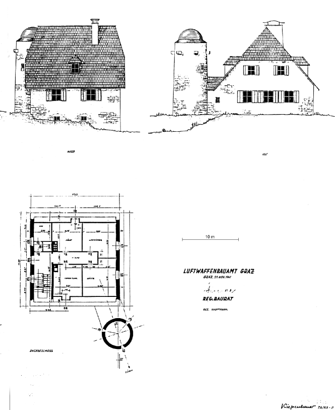
Figure 1.: Part of the original buildingplan from 1941 commissioned by the “German Luftwaffenbauamt Graz” and signed by K.O. Kiepenheuer (lower right corner).fig:plan

2 Instruments and Observations: a Historic Overview

s:instrumentation

2.1 Instrumentation

There exist two eras of instrumentation at the observatory: the time before 1973, where the main observations were performed in the southern tower (1 in Figurefig:aerial) and the era of the patrol instrument in the northern tower (2).

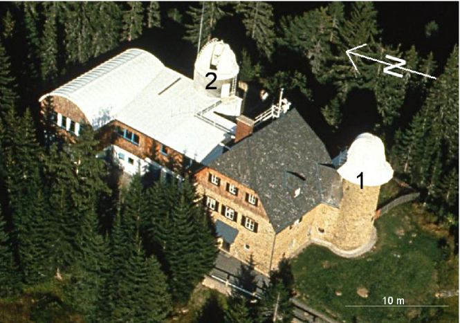
Figure 2.: Aerial view of the observatory around 1995. The original building is covered with a dark roof; the extensions were given a white roof to prevent air heating for better seeing conditions. Until 1973 the observations where performed in the southern tower (1). With the construction of the patrol instrument in the northern tower (2) the observations in the southern tower were stopped.fig:aerial

2.1.1 1943 – 1973

Northern Tower

Until 1947 a coronagraph (d/f = 11/165 cm, Comper and Kern, 1957) was installed in the northern tower. This coronagraph was then brought onto the top of the Gerlitzen mountain (1911 m a.s.l.) into the new dome constructed by the British Allied forces. It was operated there until 1964 when the observing conditons became worse due to a 25 m radio tower newly erected near the dome. Also on this coronagraph a telescope for producing sunspot drawings with a diameter of 15 cm was mounted piggyback. Until 1958 a tiny 12 cm refracting telescope with a camera was operated in this tower for night observations, which on the occasion of the International Geophysical Year (IGY) in 1958 was equipped with an H$\alpha$ monochromator from Zeiss. From this time on regular photographic H$\alpha$ observations have been made.

Southern Tower

A heliostat from Zeiss (see Figure fig:heliostat) reflected the sunlight down to the laboratory (located in the basement) where all instruments were situated. The two flat mirrors of the heliostat had a diameter of 30 cm and were guided by a synchronous motor. The mirrors were originally silver-coated, which was not a long-lasting solution. Therefore in 1950 the mirrors were coated by an aluminium evaporation deposition, which was protected by a thin silica film. In the 1960s the guiding of the heliostat was improved by installing a remote control and servomotors.

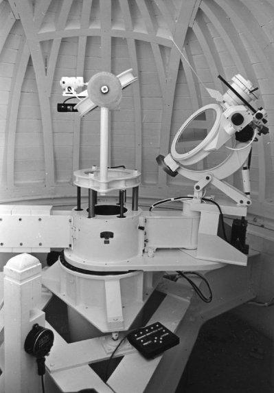
Figure 3.: The Zeiss-Heliostat with two flat mirrors of 30 cm in diameter mounted in the southern tower was in use from 1943 until 1973. The sunlight was reflected down to the laboratory in the basement, where the drawing table and the spectrohelioscope were installed.fig:heliostat

In the lower section of the tower a vertical telescope with an aperture of 11 cm and a focal length of 165 cm was mounted (Figure fig:verttelescope). This device produced a solar image of 25 cm in diameter onto a drawing board fixed on a bricklaid pedestal. Until November 1946 the vertical telescope was mounted onto the coronagraph. By changing the ocular, the projected image size was enlarged to 25 cm. The vertical telescope was pivot-mounted in order to move it out of the light path and to collimate the sunlight via a 45^∘ inclined mirror into the laboratory.

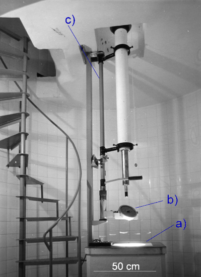
Figure 4.: The vertical telescope was mounted in the southern tower and produced a solar image with 25 cm in diameter (a). The telescope could be pivoted araund a vertical axis (c) and the light beam was reflected by a 45^∘ inclined mirror (b) into the laboratory, where the spectrohelioscope was installed.fig:verttelescope

In the laboratory basement a spectrohelioscope (Figure fig:spectrohelioscope; was operated. A schematic mode of operation of this device can be found in Siedentopf (1940) and Comper (1958)). The observations at the spectrohelioscope were made visually and the chromospheric phenomena observed in the H$\alpha$ line were added to the sunspot drawing.

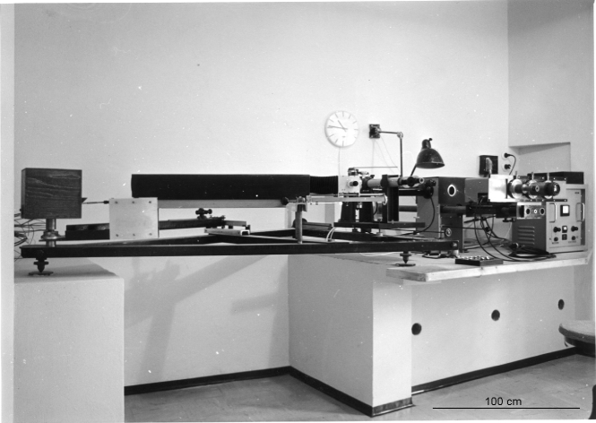
Figure 5.: In the basement laboratory a spectrohelioscope designed by Siedentopf was installed; here the Sun was observed visually in the chromospheric H$\alpha$ line and the chromospheric features were added to the sunspot drawings.fig:spectrohelioscope

2.1.2 The Patrol Instrument: 1973 – Today

The construction of the patrol instrument began in the mid 1960s during the times when the observatory was enlarged and a number of interior works and reconstructions were done, but it took until 1973 to complete the instrument and to shift the main observations there. The patrol instrument comprised three (later four) refractors on a common equatorial mounting. The diurnal movement was tracked by a microprocessor system, which was later on improved by a four-quadrant photocell controller and finally with the transfer to CCD cameras by using the solar disc image. The following instruments were mounted on the patrol instrument:
H$\alpha$ telescope: in the beginning it was equipped with a miniature film adapter that was controlled automatically so that every four minutes one image was taken. The film rolls, each consisting of about 1000 images, were completely digitized in 2007 (Pötzi, 2007). In 1998 the recording technology was changed to CCD cameras (Hanslmeier, Otruba, and Pötzi, 2003), which were upgraded in 2005 and 2010 (Pötzi et al., 2015).
Drawing device: the objective lens of the old vertical telescope was reused and a new zoom optics system was built in order to obtain the same size of the projected solar disc as before (25 cm). A great benefit was the arrangement of the drawing device directly on the declination axis of the telescope. Thus, the observers position during drawing is the same as on a lectern (see Figure fig:drawdevice) and the forces applied by the observer have minimal effects onto the telescope motion.
White-light telescope: beginning with 1989 (Pettauer, 1990) images were captured on on large size film (13 cm $\times$ 18 cm). The data and films are currently being digitized (Pötzi, 2010). In 2007 a CCD camera replaced the old system, which was again replaced in 2015 by a camera with more greylevels.
Magneto Optical Filter: this device (Cacciani et al., 1999) was only installed between 1999 and 2002, producing intensity images, dopplergrams, and magnetograms.
Ca ii K telescope: This telescope was installed in 2010; the filter is centered at 393.37 Å  and it was operated from the beginning with a CCD camera (Hirtenfellner-Polanec et al., 2011).

Table tbl:instrum gives an overview of the telescopes mounted on the patrol instrument and the corresponding data products obtained over the years. Nowadays, the following telescopes are still in use: Drawing device, H$\alpha$, white-light and Ca ii K; all are running in patrol mode observng the full-Sun with high cadence. The sunspot drawing is made once a day, it is immediately scanned to be archived in the KSO archive system (cesar.kso.ac.at).

Table 1.: Overview of the telescopes mounted on the KSO patrol instrument and their data formats. Almost all photographic data is digitized, new drawings are scanned immediately.tbl:instrum

Instrument	operating		Cadence	Size [pixel]
	from	to		greylevels
Drawing device	1973		1 per day
	(1973			1700 $\times$ 1850	digitized)
H$\alpha$	1973	2000	240 sec	photographic
	(1973	2000		1024 $\times$ 1024 / 256	digitized)
	1998	2005	100 sec	1008 $\times$ 1016 / 256
	2005	2010	10 sec	1024 $\times$ 1024 / 1024
	2010		6 sec	2048 $\times$ 2048 / 4096
White light	1989	2007	3 per day	photographic
	(1993	2007		2200 $\times$ 2200 / 32768	digitized)
	2007	2015	60 sec	2048 $\times$ 2048 / 1024
	2015		15 sec	2048 $\times$ 2048 / 4096
MOF	1999	2002	60 sec	512 $\times$ 495 / 32768
Ca ii K	2010		6 sec	2048 $\times$ 2048 / 4096

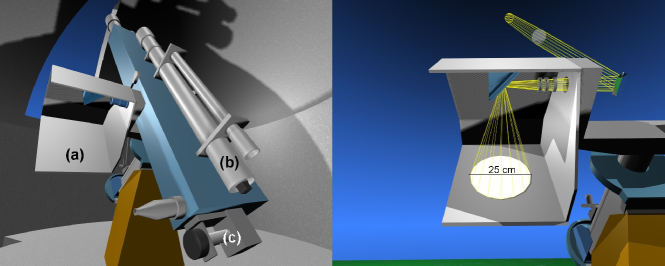
Figure 6.: Left: a schematic view of the patrol instrument comprising (a) the drawing device, (b) the white-light telescope, and (c) the H$\alpha$ telescope. Due to the mirrors, the drawing is reversed left to right and because of the light path through the declination axis of the telescope the image is also rotated by the declination angle of the Sun.fig:drawdevice

2.2 The Sunspot Drawings

2.2.1 From May 1944 until November 1946

During WW II and in the first years after the war, the sunspot drawings were made in compliance with the German system, which was specified by K.O. Kiepenheuer (see Figure fig:draw19460224). The drawings were made with a piggyback telescope on the coronagraph in the northern tower. The solar disc on the templates was 15 cm in diameter and the heliographic coordinate system was pre-printed. There existed 15 different types of heliographic coordinate templates, one for each degree of the latitude of the centre of the solar disc $B_{0}$. The grid for latitude and longitude was divided into five-degree steps. In addition to the sunspots, also plages observed in H$\alpha$ were also sketched in red.

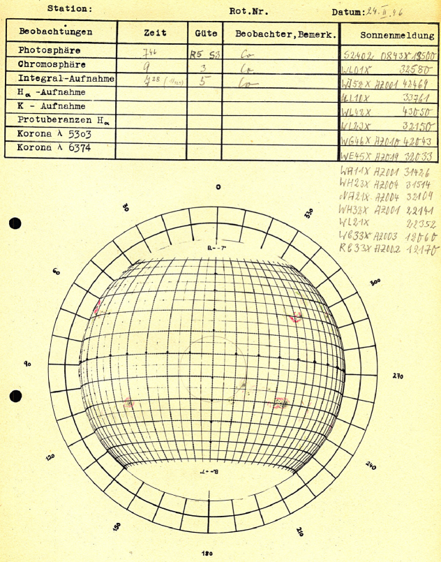
Figure 7.: Sample sunspot drawing from 24 February 1946. The German Airforce prepared heliographic coordinate sytem templates for the drawing available in one-degree steps for solar B₀ angles. Chromospheric plages were added in red.fig:draw19460224

In the header section of the sunspot drawings, the following information was given:

• Type of observation

• Time of drawing (CET), of chromosphere observation (H$\alpha$), and of white-light photograph.

• Quality for the observations, given as R (quietness) and S (sharpness) between 1 (exceptional) and 5 (very poor), defined in an internal communication by Kiepenheuer (1946).

• Name or initials of observer.

• Position and code for daily solar report (“Sonnenmeldung”).

For a later check of the sunspot numbers, the “Sonnenmeldung” is of great importance, as it is impossible today to count the sunspots on the drawings directly. The Sonnenmeldung in Figure fig:draw19460224 has to be interpreted as listed in Table tbl:code.

Table 2.: The code of the “Sonnenmeldung” consisted of information on observing time, seeing conditions, sunspot groups, and faculae observed. Here we show the interpretation of some datablocks from Figure fig:draw19460224. For each sunspot group or faculae the area of the faculae in the photosphere and chromosphere was also noted. Some identifiers could not be identified, like the first character in the first block, which can be W, P, R or T. tbl:code

Line	Datablocks			Interpretation
1	1	2	3	date	time/quality	sun spot
	S2402	0843X	19500	Feb. 24	8 MEZ	number
					photosph. 4	R = 195
					chromosp. 3
	1	2	3	type and area	sunspots	position
2	WL01X		32580	L=faculae		quadrant 3
				photosph. 0		S25W80
				chromosph. 1
3	WJ52X	AZ001	42469	J-group	1 spot	quadrant 4
				photosph. 5		N24W69
				chromosph. 2
8	WE45X	AZ019	32033	E-group	19 spots	quadrant 3
				photosph. 4		S20W33
				chromosph. 5
15	RC33X	AZ002	12170	C-group	2 spots	quadrant 1
				photosph. 3		N21E70
				chromosph. 3

2.2.2 From November 1946 until May 1973

In November 1946 a new projection lens was mounted onto the telescope in order to obtain a projection of the solar disc with 25 cm in diameter. This instrumental change from 15 to 25 cm caused an increase in sunspot detection by $\approx$50 %. In November 1947 the telescope was moved from the coronagraph to the southern tower, now called the “vertical telescope”, and the drawings were made on a stable pedestal. On the drawing templates, all sunspots, filaments, and faculae were drawn, sometimes even prominences. For the identification of chromospheric features the observer was looking through the spectrohelioscope and tried to draw these features as well as possible at the correct position of the sunspot drawing. For this purpose a rectangular grid was drawn onto the template (Figure fig:19520822). The chromospheric plages were added in red, the photospheric faculae (only near the limb) in green, the filaments and visible lower parts of prominences were sketched in grey.
Until 1957, the sunspot numbers were also derived separately for the central zone, i.e. sunspots inside half of the solar radius. Until 1948 seeing conditions were not taken into account for deriving the sunspot number. With the beginning of the year 1952, the observation time was changed from CET to UT.

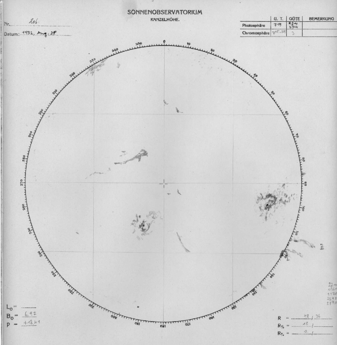
Figure 8.: Sunspot drawing from 22 August 1952: Besides the sunspots, also chromospheric plages (around sunspots), photospheric faculae, and filaments were drawn. The chromospheric features were detected visually at the spectrohelioscope in the H$\alpha$ spectral line. In order to draw these features onto the correct place a grid was added. Sometimes the locations and time of flares were also added.fig:19520822

2.2.3 From May 1973 To Date

From May 1973 to date the sunspot drawings have been made at the patrol instrument in the northern tower (Figure fig:drawing). Chromospheric features are no longer added to the drawings as in parallel the photographic patrol observations in H$\alpha$ began (Pötzi, 2007).

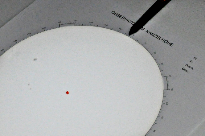
Figure 9.: A drawing template fixed in the drawing device. The red dot in the centre of the solar image is the needle, which is stuck into the template through the solar disc centre. The black arrow shaped holder in the upper part of the image fixes the template at the negative declination angle of the Sun.fig:drawing

2.3 International Cooperations

Until 1945 the main cooperation took place with Freiburg and the newly founded network of German observatories (Seiler, 2007; Jungmeier, 2014). After WW II the southern part of Austria was occupied by the British allied forces. A continuation of the cooperation with Freiburg was hardly possible as it was located in Germany. The local staff at KSO got into contact with the Astronomer Royal from the Greenwich Observatory, which led to a fruitful cooperation and secured the existence of the observatory. According to the Greenwich Royal Observatory in 1947, the cooperation with Greenwich had already begun in 1946. The cooperation with other institutes began in 1948 according to the KSO activity reports (KSO, 1946 – 2000). Sunspot numbers were sent to Freiburg each month, quarterly copies of sunspot drawings were sent to Zurich, and flare data were sent to Meudon, France. From 1957 on, the International Geophysical Year (IGY), data were sent to Freiburg every 14 days, to Meudon, Pic du Midi, Boulder, and Moscow every month, and quarterly to Zürich (Mathias, 1962; Haupt, 1971). The activity reports contain no information about the cooperation with Greenwich, which seems to have stopped with the end of the occupation of Austria by the Allied forces in 1955.
With new technologies (Telex in the 1970s and later internet) the data transfer to other institutes and data centres was improved and became more frequent. Nowadays the sunspot number is sent directly to the SILSO database (Sunspot Index and Long-term Solar Observations in Belgium), and the H$\alpha$ patrol images are sent every night to the Global High Resolution H-alpha Network (Steinegger et al., 2000) at the New Jersey Institute of Technology. Flare reports and patrol times are sent on a monthly basis to the National Centers for Environmental Information (NCEI), USA. Long-exposure H$\alpha$ images showing off-limb prominence structures are sent to AISAS (Astronomical Institute of the Slovak Academy of Sciences) as a supplement for the Lomnicky Stit prominence catalogue (Rybák et al., 2011). Web sites such as solarmonitor.org display the Kanzelhöhe solar images. H$\alpha$ live images and real-time flare detections are provided via ESA’s Space Weather Portal (swe.ssa.esa.int). Additionally all observational data is also available via the online archive of the Kanzelhöhe Observatory cesar.kso.ac.at (Pötzi, Hirtenfellner-Polanec, and Temmer, 2013).

3 Sunspot Numbers Derived at KSO

The sunspot groups are classified according to the Zurich classification scheme (Waldmeier, 1955), which describes the evolution of sunspot groups. The relative sunspot number is then obtained by counting the individual sunspots [s] and sunspot groups [g] as:

$$R=k(10\cdot g+s)$$

The reduction factor [$k$] is a weighting factor that accounts in particular for the different telescopes, which is necessary when combining the data of different observatories. Until 2015 this factor was set to match the original 8 cm telescope with a magnification of 64 used by Rudolf Wolf in Zürich (Waldmeier, 1961). For the ISN a reduction factor for each telescope is calculated, regardless of the observer and the observational conditions. But in principle for each observer an individual reduction factor can be applied.

3.1 Reduction Factor $k$ at KSO

The atmosphere of the Earth influences the observation conditions. Air turbulence, clouds, and wind have an impact on the quality; even a clear sky is not a guarantee for good seeing. Haupt (1965) compared seeing conditions at KSO depending on general weather situations. He showed, e.g., that the worst conditions occur when there is an upper air flow from the North and a clear blue sky. Generally the best observing conditions are in the early morning, before the Sun heats up the ground, and also when there are very thin high cloud layers.
The quality of the observations can be described by two main factors: the sharpness and the quietness. At KSO the sharpness and the quietness have been used according to an internal communication by Kiepenheuer (1946) and redefined in Kiepenheuer (1964). The sharpness is defined as numbers between 1 and 5 in steps of 0.5 depending on the details visible in the solar photosphere, e.g., 1 means that the granulation is clearly visible and even details inside the umbra can be observed, whereas at a sharpness of 3 the granulation pattern is no longer recognizable. The quietness, also between 1 and 5, describes the image motion inside the sunspots and at the limb, e.g., 1 stands for a completely stable image and at 3 the image motion is well visible on disc and at the limb but less than 4 arcsec. The quality of the observation is defined via the sharpness, as this parameter most strongly affects the number of visible sunspots. Low quietness makes the act of sunspot drawing more difficult as the projection is shaking. If the sharpness and the quietness become worse, the number of sunspots that can be identified decreases, especially small A-spots are no longer visible. On the other hand, the number of big H-spots is not affected by the seeing. However, on average the number of observed sunspots increases with better seeing quality. In order to obtain sunspot numbers that are stable (in time) and comparable (among different observatories) reduction factors for the seeing conditions have been introduced. Figure fig:corr shows how these reduction factors influence the raw sunspot number (red): If the quality (sharpness) is below 2 the corrected relative sunspot number (green) is smaller, whereas in the other cases the corrected relative sunspot number is larger than the raw relative number (blue). In general the dispersion of the daily relative sunspot numbers is reduced by the application of the reduction factor [$k$].

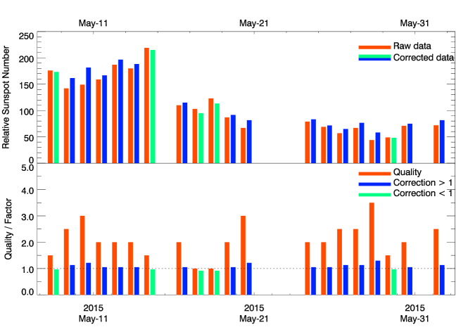
Figure 10.: Influence of the seeing conditions on the relative sunspot number derived. In the lower panel the image quality for each day and the corresponding correction factor is plotted. In the upper panel the raw relative sunspot numbers (red) and the corrected sunspot numbers are plotted side by side. Blue (green) indicates relative sunspot numbers that are higher (lower) then the raw data.fig:corr

In the first years until 1948 the relative sunspot numbers obtained from the sunspot drawings have not been reduced. In 1948, Anton Bruzek (head of the observatory and observer during the years 1947 to 1953) made a first attempt to derive the reduction factors for the local observations (KSO, 1946 – 2000). For this purpose he analysed all relative sunspot numbers obtained at KSO from 1946 to 1948 and classified them according to the quality into classes from 1 to 5. He assumed that the relative sunspot numbers in each class should be homogeneously distributed, i.e. the mean sunspot number in each class should be the same, if there was no influence by seeing conditions. With this method he calculated the correction factors between the different classes. In a first step he set the reduction factor for quality 3 to 1.0. In order to connect the local observations at KSO to the international sunspot numbers he used the observations from Zürich, Freiburg and the American Relative Sunspot Numbers [$R_{a}$: Shapley, 1949]. As the number of observations in the classes 1 and 5 was very low, these factors are the most uncertain ones. Table tbl:factor lists the reduction factors used at KSO since 1946. In the first two years (1944 – 45) no reduction factors were applied. Due to instrumental changes the factors had to be recalculated twice, the first time in 1958 (Haupt, Ellerböck, and Kern, 1959) and then again in 1979 (Schroll, 1979). Both times the recalculation was delayed by some years as there was a solar minimum and thus not enough days available with high relative sunspot numbers to obtain good statistics. In 2015 with the recalibration of the relative sunspot numbers by Clette et al. (2014) the ISN was adjusted to modern telescopes, i.e. the ISN was not only corrected for e.g., the transition form Wolf to Wolfer (factor 1.67) or Zürich weighting after 1947 (-18%), but also the whole series was divided by 0.6.

Table 3.: KSO reduction factors [$k$] for the observed sunspot numbers according to the seeing conditions. The initial $k$ factors were calculated in 1948, and were updated twice (in 1958, 1979) to account for instrumental changes. The update in 2015 (multiplication of $k$ by $\frac{5}{3}$) is due to the recalibration of the ISN by Clette et al. (2014). In the table we list the factors, the total numbers of sunspot drawings for each quality class and for the period of 1946 to 1948 the mean sunspot number of each quality class.tbl:factor

Quality	1	1 – 2	2	2 – 3	3	3 – 4	4	4 – 5	5
total (1946 – 1948)	3		44		134		121		35
$\overline{R}$	390		288		222		180		150
$k$ (1948)	0.38	0.46	0.52	0.59	0.67	0.75	0.86	0.97	1.00
total (1955 – 1957)		2	19	57	181	232	205	73	85
$k$ (1958)	0	0.55	0.63	0.71	0.79	0.87	0.95	1.02	1.10
total (1973 – 1978)		100	368	272	212	146	77	32	34
$k$ (1979)	0.55	0.59	0.63	0.68	0.73	0.79	0.85	0.92	0.99
$k$ (2015)	0.92	0.98	1.05	1.13	1.22	1.32	1.42	1.53	1.65

Figure fig:seeing plots the yearly running mean image quality from 1945 to 2015, illustrating the change of the seeing conditions at KSO over the past seven decades of observations. After 25 years of quite unstable conditions until around 1970 they became more stable for almost 30 years. From 2000 on, both the sharpness and the quietness of the images improved by at least half of a class. In Figure fig:seeing rapid changes in the quality are marked with ellipses and numbers and are discussed below:

• Due to the increase of the size of the projected image from 15 cm to 25 cm in Nov. 1946, a larger number of sunspots could be identified in the observations. As the projection changed from the piggyback instrument on the coronagraph to the projection in the southern tower in the year 1948 with a stable drawing table the quality of the observation further improved.

• According to the activity reports there were problems with the guiding of the heliostat in 1948 and problems with the aluminium coating of its mirrors. In the year 1950 a completely new coating of the mirrors enhanced the brightness and therefore the contrast and quality of the projection.

• The quality of the mirrors degraded and due to the minimum of the solar cycle there were only a few sunspots visible, which makes a good estimation of the image quality difficult.

• For the low quality values in 1957 – 58 no instrumental cause could be found in the activity reports. During this period the KSO observers detected a strong deviation of the local sunspot numbers from Zurich and Freiburg, and therefore they recalculated the reduction factors.

• Time of major reconstruction works at the observatory and a period of frequent replacement of personnel. This can be seen in Figure fig:newobs, where we plot for each year the total number of observers as well as the newly instructed observers. In the year 1965 many trees around the observatory were cut, especially in the principal wind direction, which may have led to better seeing conditions. Some modifications at the end of the year 1966 in the southern tower led to improved observation conditions as the airflow changed.

• For a few years the seeing conditions became worse as a result of the Pinatubo volcano eruption in June 1991 (Otruba, 1993).

• This increase in quality cannot be explained by improvements of the instrumentation or by any changes in the vicinity of the observatory. We may speculate that climatic changes led to different atmospheric influences, but according to Auer et al. (2007) massive changes in temperature and air humidity in southern Austria had already begun in 1970.

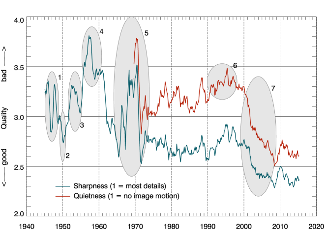
Figure 11.: Yearly running mean of sharpness and quietness values of the last 7 decades, the quietness is almost proportional to the sharpness. The ellipses mark times, when major changes in the observational conditions occurred.fig:seeing

3.2 Comparison of the Kanzelhöhe Relative Number to the ISN

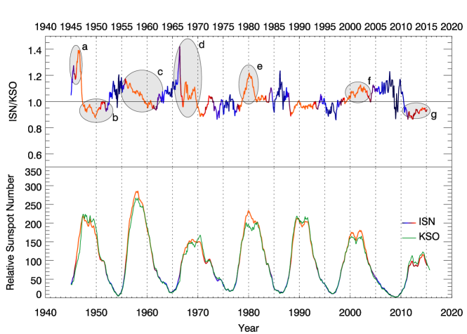
Figure 12.: Top: Ratio of the 13-month running mean of the recalibrated ISN (SILSO World Data Center, 1945 – 2015) to KSO sunspot numbers. Values greater than unity indicate that the ISN is higher than the KSO sunspot number. The color changes from blue to red for relative sunspot numbers above 100, i.e. solar activity minima are blue. Bottom: Relative sunspot numbers from KSO (green) and ISN (blue – red) from 1945 to 2015.fig:kso˙sidc

Figure fig:kso_sidc shows the 13-month running mean sunspot numbers derived at the KSO together with the International Sunspot Numbers (ISN; Silso World data Center, SILSO World Data Center (1945 – 2015)) for the period 1945 to 2015. The top panel shows the ratio of the two time series. In general both time series agree within a limit of $\approx$20 % (with two exceptions). The mean of the ratio of the ISN to the KSO sunspot numbers is 1.025 $\pm$ 0.088, i.e. the rms differencees are at a level of 9 %. In Figure fig:kso_sidc, we also indicate periods of larger deviations. However we do not consider relative differences at solar activity minima (blue), as the small sunspot numbers may lead to relatively large deviations in the relative differences although the absolute agreement is very high. We note the following periods of larger ($\gtrsim$10 %) deviations:

• The same reasons as above in items 1 and 2 apply here. Additionally Anton Bruzek introduced a new reduction factor.

• The drift between 1956 and 1962 cannot be explained by any instrumental changes. In 1958 new correction factors were calculated as it became clear that there was some deviation; these factors were higher and may be the reason for the extension of the drift until 1962.

• Between 1965 and 1968 major construction works were carried out at the observatory, the observations were even stopped for some months in 1966, 1967, and 1968. A fluctuation of observers began in 1968, when three new observers were employed. These fluctuations lasted until 1975 with a total of ten new observers (Figure fig:newobs).

• New reduction factors were used from June 1979 on, which led to smaller sunspot numbers. The new $k$-factors for qualities 3 to 5 were about 10 % lower than the old factors (cf. Tab. tbl:factor); therefore, as the mean quality was above 3, these factors should be responsible for a reduction of only 10 %. This deviation maybe due to the fact that there is also some uncertainty in the ISN series during this time as there was the closing of the Zurich observatory and the transition to Locarno as reference (Clette et al., 2014).

• New observers were employed but also sudden image quality changes happened (see Figure fig:seeing). Two observers went into retirement; their eyesight may have become worse causing some drift in the sunspot number, similar to the reason for the Locarno drift discussed in Clette et al. (2014).

• From 2009 new observers came to the observatory and were introduced into the observational work. New observers tend to underestimate the image quality which results in higher sunspot numbers. Figure fig:seeing_start shows how on average the image quality is estimated over the first two years by new observers; the estimation is nearly half a class worse at the beginning of their career as observer.

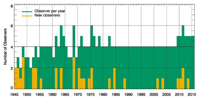
Figure 13.: The total number of observers for each year (green) and the number of newly employed observers (yellow). On average, four observers are needed for continuous observations, i.e. also on weekends and holidays. In former times fewer observers were necessary, as the weekly working time was 48 hours until 1958 and then step by step reduced to 40 hours in 1979.fig:newobs

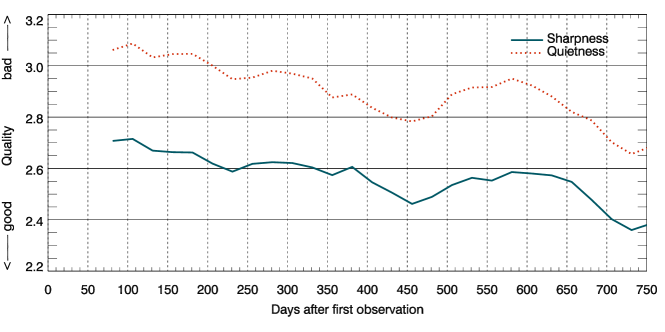
Figure 14.: Mean sharpness and quietness estimates derived from all individual observers who contributed with more than 100 drawings (total number 21) during their first two years of observing duty. The data is smoothed over half a year. Both values are higher in the first few months. An underestimate of the image quality causes an overestimate of the sunspot numbers.fig:seeing˙start

4 Discussion

In general, the sunspot numbers derived at KSO and the ISN reveal a good agreement. The mean of the ratio of the ISN/KSO monthly mean sunspot numbers for 1945 – 2015 is 1.025 $\pm$ 0.088. However, there are a few periods where the relative difference exceeds $\pm$ 20 % (28 months out of 842). The main reasons for these large differences are instrumental improvements and observer fluctuations. For some periods with major deviations (e.g. around 1980) no explanation could be found.

An important factor in determining the Sunspot Number is the group number (Hoyt and Schatten, 1998a, b), as each group counts as much as ten individual sunspots. A few years after the reduction factors of the new patrol instrument were recalculated by Schroll (1979) he found out that there was still a large deviation from the ISN. His assumption was that the number of groups could be too low as a result of assigning too many sunspots to one group or the insufficient detection of small groups. Fig fig:kso_sidc shows that around 1990 the KSO sunspot numbers agree well with the ISN, but inspection of Figure fig:groups shows that especially in this time the number of detected sunspot groups was considerably higher at KSO. In 1980, when the KSO sunspot numbers were too low by $\sim$20%, the number of sunspot groups detected at KSO was identical to the ISN sunspot group number. The right panel in Figure fig:groups shows an extreme example of group splitting; another observer could have found only three groups in the same drawing, as it is not always clear how to split these groups. It was drawn at a time when a video system was installed at the observatory that displayed a live H$\alpha$ image, which made it easier to find the individual active regions. In the last years this has become much easier, spaceborne instruments such as the Solar and Heliospheric Observatory (SOHO) or the Solar Dynamics Observatory (SDO) provide the observers with high resolution images in various wavelengths and additionally with magnetic maps. Using such additional data is actually also a change in the method and could lead to differences in the sunspot numbers derived that are no longer comparable to the long time sunspot data series anymore.

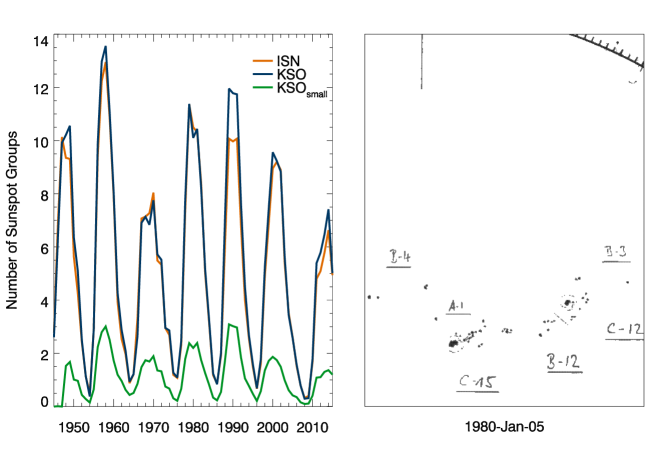
Figure 15.: Left: Comparison of yearly group numbers between the international (red, Svalgaard and Schatten (2015)) and KSO (dotted blue) group numbers. In dashed green we plot the yearly average number of small groups, i.e. A-1 to A-3, B-2 and B-3. In the right panel there is a display detail of a drawing showing the splitting of groups.fig:groups

When new observers are trained, we have noticed that they try to do their best, and they often tend to find more small sunspots than there are actually on the solar disc. In cases of very good seeing conditions, they are not really able to distinguish between small sunspots and pores or big dark intergranular regions. On the other hand, they also tend to overlook new spots close to the limb. In the KSO database there is an extra entry for small sunspot groups, i.e. sunspot groups of the classes A-1 to A-3, B-2 and B-3. This number is also plotted in Figure fig:groups (green) in addition to the total group numbers. This plot shows that the number of small sunspots is proportional to the total group number. Before 1947 small sunspot groups are missing due to the projection size of only 15 cm and around 1990 a large number of small sunspot groups where detected at KSO. However, especially around 1990 there was no change in the observing team.

Starting with the IGY (1958) until 1964, each observatory got a certain time slot for intensified observations. The observers were complaining that they had to observe around Noon, which was very late as the seeing conditions are the best early in the morning. As the KSO operates a meteorological station for the Central Institute for Meteorology and Geodynamics (ZAMG) hourly sunshine information is available for all years. These sunshine data show that on average the Sun shines two hours before the drawing is made. This value did not increase during the IGY, so only the chromospheric observations were shifted to the determined time slot. The image quality even improved during this time (Figure fig:seeing). Only between 1966 and 1970 was the sunshine duration more than three hours before drawing the sunspots, which was probably a result of the personnel situation in this period. For three months in 1969 there was only one person at the observatory. The relatively bad seeing conditions reported during this period may thus be related to the fact that the sunspot observations were carried out one hour later than in general. In additon to the later observation time the fluctuation of observers, the construction works, and the cutting of trees in the surrounding of the observatory may also have affected the quality estimation.

Another impact could come from climatic changes; in the southern part of Austria the air became dryer and the temperature rose by about one degree over the last 40 years (Auer et al., 2007) and according to the studies of Haupt (1965) also the general weather situation influences the image quality. Figure 54 of Clette et al. (2014) shows the variation of the annual average quality index of Locarno. There the construction of a building near the observatory led to a quality jump but there appears to be a slow change to lower quality values over the last 45 years.

We conclude that the relative sunspot number derived at KSO is in good agreement with the ISN; there is no long-term drift between the two numbers. However, there are also periods with larger deviations that can be explained by new personnel, instrumental changes, or modifications in the vicinity, and there are also periods of deviations for which no reason was found. As the $k$ factors also depend on the observers themselves, they should be recalculated and verified at regular intervals, especially when an observing team does not change for a longer period of time.

Disclosure of Potential Conflicts of Interest

The authors declare that they have no conflicts of interest.

Acknowledgments

Many pieces of information about historical and instrumental details were not available in printed or written form. We are grateful to Hermann Haupt and Thomas Pettauer, who have shaped the observatory through their work since the early 1950s and 1960s, respectively, for all of the information that they provided us through private communications that would have been lost otherwise.

References

- Auer et al. (2007) Auer, I., Böhm, R., Jurkovic, A., Lipa, W., Orlik, A., Potzmann, R., Schöner, W., Ungersböck, M., Matulla, C., Briffa, K., Jones, P., Efthymiadis, D., Brunetti, M., Nanni, T., Maugeri, M., Mercalli, L., Mestre, O., Moisselin, J.-M., Begert, M., Müller-Westermeier, G., Kveton, V., Bochnicek, O., Stastny, P., Lapin, M., Szalai, S., Szentimrey, T., Cegnar, T., Dolinar, M., Gajic-Capka, M., Zaninovic, K., Majstorovic, Z., Nieplova, E.: 2007, HISTALP - historical instrumental climatological surface time series of the Greater Alpine Region. Int. J. Climatology 27, 17. DOI. ADS.
- Cacciani et al. (1999) Cacciani, A., Moretti, P.F., Messerotti, M., Hanslmeier, A., Otruba, W., Pettauer, T.V.: 1999, The Magneto-Optical Filter at Kanzelhöhe. In: Hanslmeier, A., Messerotti, M. (eds.) Motions in the Solar Atmosphere, Astrophysics and Space Science Library 239, 271. ADS.
- Clette et al. (2014) Clette, F., Svalgaard, L., Vaquero, J.M., Cliver, E.W.: 2014, Revisiting the Sunspot Number. A 400-Year Perspective on the Solar Cycle. Space Sci. Rev. 186, 35. DOI. ADS.
- Comper (1958) Comper, W.: 1958, Die eruptive Protuberanz vom 16. Dezember 1956. Mit 9 Textabbildungen. ZAp 45, 83. ADS.
- Comper and Kern (1957) Comper, W., Kern, R.: 1957, Die Eruption (Flare) und der Protuberanzenaufstieg vom 4. Juni 1956. Mit 4 Textabbildungen. ZAp 43, 20. ADS.
- Dellinger (1935) Dellinger, J.H.: 1935, A New Cosmic Phenomenon. Science 82, 351. DOI. ADS.
- Eckel and Lauscher (1937) Eckel, O., Lauscher, F.: 1937, Vom Klima der Kanzelhöhe. Carinthia II 127, 1.
- Greenwich Royal Observatory (1947) Greenwich Royal Observatory: 1947, Report of the proceedings of the Greenwich Royal Observatory. MNRAS 107, 62. ADS.
- Hanslmeier, Otruba, and Pötzi (2003) Hanslmeier, A., Otruba, W., Pötzi, W.: 2003, New H instrumentation at the Kanzelhöhe Solar Observatory. In: Wilson, A. (ed.) Solar Variability as an Input to the Earth’s Environment, ESA Special Publication 535, 729. ADS.
- Haupt (1965) Haupt, H.: 1965, Die Qualität der Sonnenbeobachtungen auf der Kanzelhöhe in Abhängigkeit von der Großwetterlage. Carinthia II 24, 290.
- Haupt (1971) Haupt, H.: 1971, Astronomisches Institut (Universitäts-Sternwarte). I. Universitäts-Sternwarte Graz. Report 1969-1970. II. Sonnenobservatorium Kanzelhöhe. Report 1963-1970. Mitteilungen der Astronomischen Gesellschaft Hamburg 29, 62. ADS.
- Haupt, Ellerböck, and Kern (1959) Haupt, H., Ellerböck, W., Kern, R.: 1959, Die Abhängigkeit der am Sonnenobservatorium Kanzelhöhe beobachteten Sonnenfleckenrelativzahlen von Luftgüte und Klassifizierung. Anzeiger der Math.-naturwiss. Klasse der Österr. Akademie der Wissenschaften 12, 237.
- Hirtenfellner-Polanec et al. (2011) Hirtenfellner-Polanec, W., Temmer, M., Pötzi, W., Freislich, H., Veronig, A.M., Hanslmeier, A.: 2011, Implementation of a Calcium telescope at Kanzelhöhe Observatory (KSO). Central European Astrophysical Bulletin 35, 205. ADS.
- Hoyt and Schatten (1998a) Hoyt, D.V., Schatten, K.H.: 1998a, Group Sunspot Numbers: A New Solar Activity Reconstruction. Sol. Phys. 179, 189. DOI. ADS.
- Hoyt and Schatten (1998b) Hoyt, D.V., Schatten, K.H.: 1998b, Group Sunspot Numbers: A New Solar Activity Reconstruction. Sol. Phys. 181, 491. DOI. ADS.
- Jungmeier (2014) Jungmeier, G.: 2014, “… für eine dauernde Überwachung der Vorgänge auf der Sonne zum Zwecke der Funkberatung …”. http://kso.ac.at/praesentation/fuer˙eine˙dauernde˙ueberwachung.pdf. Accessed: 2015-12-07.
- Jungmeier, Veronig, and Pötzi (2014) Jungmeier, G., Veronig, A., Pötzi, W.: 2014, Sonnenforschung auf der Kanzelhöhe. Sterne und Weltraum.
- Kiepenheuer (1946) Kiepenheuer, K.O.: 1946, Internal Communications. Archives of the Kanzelhöhe Observatory, internal.
- Kiepenheuer (1964) Kiepenheuer, K.O.: 1964, Solar Site Testing. In: Rosch, J. (ed.) Le choix des sites d’observatoires astronomiques (site testing), IAU Symposium 19, 193. ADS.
- KSO (1946 – 2000) KSO: 1946 – 2000, Tätigkeitsberichte des Observatoriums Kanzelhöhe. Archives of the Kanzelhöhe Observatory, internal.
- Kuiper (1946) Kuiper, G.P.: 1946, German astronomy during the war. Popular Astronomy 54, 263. ADS.
- Mathias (1962) Mathias, O.: 1962, Das Sonnenobservatorium der Universität Graz auf der Kanzelhöhe (Tätigkeitsbericht für die Jahre 1946 bis 1962). Anzeiger der Math.-naturwiss. Klasse der Österr. Akademie der Wissenschaften, 232.
- Otruba (1993) Otruba, W.: 1993, Sky Darkening in Central Europe due to the Pinatubo Eruption. Anzeiger der Math.-naturwiss. Klasse der Österr. Akademie der Wissenschaften 130.
- Pettauer (1990) Pettauer, T.: 1990, The Kanzelhöhe photoheliograph. Publications of Debrecen Heliophysical Observatory 7, 62. ADS.
- Pötzi (2007) Pötzi, W.: 2007, Scanning the old H films at Kanzelhöhe. Central European Astrophysical Bulletin 2, in press. ADS.
- Pötzi (2010) Pötzi, W.: 2010, Digitizing the KSO white light images. Central European Astrophysical Bulletin 34, 1. ADS.
- Pötzi, Hirtenfellner-Polanec, and Temmer (2013) Pötzi, W., Hirtenfellner-Polanec, W., Temmer, M.: 2013, The Kanzelhöhe Online Data Archive. Central European Astrophysical Bulletin 37, 655. ADS.
- Pötzi et al. (2015) Pötzi, W., Veronig, A.M., Riegler, G., Amerstorfer, U., Pock, T., Temmer, M., Polanec, W., Baumgartner, D.J.: 2015, Real-time Flare Detection in Ground-Based H Imaging at Kanzelhöhe Observatory. Sol. Phys. 290, 951. DOI. ADS.
- Rybák et al. (2011) Rybák, J., Gömöry, P., Mačura, R., Kučera, A., Rušin, V., Pötzi, W., Baumgartner, D., Hanslmeier, A., Veronig, A., Temmer, M.: 2011, The LSO/KSO H prominence catalogue: cross-calibration of data. Contributions of the Astronomical Observatory Skalnate Pleso 41, 133. ADS.
- Schroll (1979) Schroll, A.: 1979, Neubestimmung der Reduktionsfaktoren für die Sonnenfleckenbeobachtungen des Sonnenobservatoriums Kanzelhöhe. Sitzungsbericht der Österr. Akademie der Wiss. Mathem.-naturwiss. Klasse Abteilung II 188, 256.
- Seiler (2007) Seiler, M.P.: 2007, Covert Operation ”Sun God” - History of German Solar Research in the Third Reich and Under Allied Occupation (German Title: Kommandosache ”Sonnengott” - Geschichte der deutschen Sonnenforschung im Dritten Reich und unter alliierter Besatzung). Acta Historica Astronomiae 31. ADS.
- Shapley (1949) Shapley, A.H.: 1949, Reduction of Sunspot-Number Observations. PASP 61, 13. DOI. ADS.
- Siedentopf (1940) Siedentopf, H.: 1940, Ein Spektrohelioskop mit Konkavgitter. Mit 1 Abbildung. ZAp 19, 154. ADS.
- SILSO World Data Center (1945 – 2015) SILSO World Data Center: 1945 – 2015, The International Sunspot Number. International Sunspot Number Monthly Bulletin and online catalogue. ADS.
- Steinegger et al. (2000) Steinegger, M., Denker, C., Goode, P.R., Marquette, W.H., Varsik, J., Wang, H., Otruba, W., Freislich, H., Hanslmeier, A., Luo, G., Chen, D., Zhang, Q.: 2000, The New Global High-Resolution H Network: First Observations and First Results. In: Wilson, A. (ed.) The Solar Cycle and Terrestrial Climate, Solar and Space weather, SP-ESA, Noordwijk 463, 617. ADS.
- Svalgaard and Schatten (2015) Svalgaard, L., Schatten, K.H.: 2015, Reconstruction of the Sunspot Group Number: the Backbone Method. ArXiv e-prints. ADS.
- Waldmeier (1955) Waldmeier, M.: 1955, Ergebnisse und Probleme der Sonnenforschung. ADS.
- Waldmeier (1961) Waldmeier, M.: 1961, The sunspot-activity in the years 1610-1960. ADS.