Measurement induced nonclassical states from coherent state heralded by Knill-Laflamme-Milburn-type SU(3) interference

Abstract

We theoretically generate nonclassical states from coherent state heralded by Knill-Laflamme-Milburn (KLM)-type SU(3) interference. Injecting a coherent state in signal mode and two single-photon sources in other two auxiliary modes of SU(3) interferometry, a broad class of useful nonclassical states are obtained in the output signal port after making two single-photon-counting measurements in the two output auxiliary modes. The nonclassical properties, in terms of anti-bunching effect and squeezing effect as well as the negativity of the Wigner function, are studied in detail by adjusting the interaction parameters. The results show that the input coherent state can be transformed into non-Gaussian states with higher nonclassicality after measurement induction. The maximum squeezing of our generated states can be arrived at about 1.9 dB.

PACS: 03.67.-a, 05.30.-d, 42.50,Dv, 03.65.Wj

Keywords: nonclassical state; non-Gaussian state; SU(3) interference; linear optics; mesurement-induced; Wigner function

I Introduction

Nonclassical optical states, as the basic sources, play essential roles in continuous variables (CV) quantum information processing (QIP) 1 ; 2 . Quantum information over CVs has yielded many exciting advances, both theoretically and experimently, in fields such as quantum teleportation 3 ; 4 , quantum metrology 5 , and potentially quantum computation 6 ; 7 . In order to enhance performance to implement various tasks and provide quantum advantages not attainable classically, a number of world-wide groups has embarked on route towards understanding, generating, and ultimately manipulating various nonclassical states of light 8 . In recent years, many types of nonclassical states have been proposed in theory and even have already been implemented in laboratories. Agarwal and Tara generated a nonclassical state by operating photon addition on a coherent state and investigated the non-classicality of field states 9 . Zavatta et al. had realized the single-photon added coherent state 10 and single-photon-added thermal state 11 .

Gaussian states play a prominent roles in CV quantum information 12 ; 13 . However, many quantum technological protocols, such as entanglement distillation 14 ; 15 or quantum error correction 16 , necessarily require the use of non-Gaussian state, which can extract ultimate potential of quantum information theory unaccessible by the Gaussian states. With the increasing significance of non-Gaussian states, the issues of generating non-Gaussian states have been naturally arisen. It is well-known that the non-Gaussian states must exhibit non-Gaussian features in their Wigner distributions in the phase space 17 and gererating non-Gaussian states normally requires nonlinearities in the field operators 18 . In order to obtain non-Gaussian states, there is an alternative idea of measurement-induced scheme (also the conditional probabilistic operation) to obtain nonlinearity 19 . Some effective nonlinearity 20 is associated with non-Gaussian measurement such as homodyne measurements or photon countings 21 ; 22 based on a linear quantum-optical system 23 , which generally consist of beam splitting, phase shifting, squeezing, displacement, and various detection 24 .

Many examples of such measurement-induced schemes by linear optics have been theoretically implemented, where nonlinear operators are obtained and then non-Gaussian states are generated 25 ; 26 . Dakna et al. generated a Schrodinger-cat-like state from a single-mode squeezed vacuum state by subtracting photons with low reflectance beam-splitters (BSs) and photon counters 27 . Subsequently, Lvovsky and Mlynek proposed the idea of “quantum-optical catalysis” and generated a coherent superposition state $t\left|0\right\rangle+\alpha\left|1\right\rangle$ 28 . This state was generated in one of the BS output channels if a coherent state $\left|\alpha\right\rangle$ and a single-photon Fock state $\left|1\right\rangle$ are present in two input ports and a single photon is registered in the other BS output. They called this transformation as “quantum-optical catalysis” because the single photon itself remains unaffected but facilitates the conversion of the target ensemble. Following Lvovsky and Mlynek’s work and using “quantum-optical catalysis”, Bartley et al. further generated multiphoton nonclassical states via interference between coherent and Fock states, which exhibit a wide range of nonclassical phenomena 29 . Indeed, the key step in Bartley’s scheme is to employ “quantum-optical catalysis” on the input coherent state one time. Recently, we operated “quantum-optical catalysis” on each mode of the two-mode squeezed vacuum state and generated a non-Gaussian two-mode quantum state with higher entanglement, accompanied by a nonlinear operator $c_{0}\allowbreak+c_{1}a^{{\dagger}}b^{{\dagger}}+c_{2}a^{{\dagger}2}\allowbreak b^{{\dagger}2}$ 30 . Enlighten by above works, we further consider the following problem: If we perform “quantum-optical catalysis” on a coherent state two times, then what states will be generated and what nonclassical phenomena will happen? This is the kernal focus of our work.

In 2000, Knill, Laflamme, and Milburn (KLM) implemented a nonlinear sign (NS) change using a optical network composed of three beam splitters in succession, whose main features are the use of two ancilla modes with one prepared photon and post-selection based on measuring the ancillas 31 . Because of the SU(3) algebra property of this setup, we name it as KLM-type SU(3) interferometry. Following KLM’s program and using KLM-type SU(3) interferometry, Ralph et al. constructed a conditional quantum control-NOT gate from linear optical elements 32 . Laterly, Scheel et al. investigated the generation of nonlinear operators and constructed useful single-mode and two-mode quantum gates necessary for all-optical QIP 33 . Hence we also use the KLM-type SU(3) interferometry as our framework to generate nonclassical states.

In this paper, based on the network of KLM-type SU(3) interferometry, we generate a broad class of nonclassical states from a coherent state by operating two-fold “quantum-optical catalysis”, a kind of measurement-induced scheme. Special attention is paid to study the nonclassical properties for the generated states in terms of anti-bunching effect and squeezing effect as well as the negativity of the Wigner function. We show that the input coherent state can be transformed into non-Gaussian states with higher nonclassicality after measurement induction. The paper is organized as follows. In section II, We briefly outline the KLM-type SU(3) interferometry and introduce the measurement-induced scheme for generating nonclassical states. In particular, the normalization factor (i.e. success probability) is discussed. In section III, we investigate the nonclassical properties (anti-bunching effect and squeezing effect) of the generated state and analyze the effect of the interaction. Then in section IV we consider the negativity of the Wigner function, another nonclassical indication for a quantum state. We summarize our main results in Sec.V.

II Measurement induced nonclassical state

In this section, we briefly outline the dynamics of KLM SU(3) interferometry and apply this interferometry to generate nonclassical states by measurement-induced protocol. The theoretical scheme is proposed and the success probability is derived.

II.1 KLM-type SU(3) interferometry

Linear optical networks have important applications in QIP and can be realized in experiment 34 . The quantum mechanical description of linear optics can be found in Ref 35 . Recently, there has been a growing interest in linear optical networks in the context of quantum information technology. It has been demonstrated that universal (nondeterministic) quantum computation is poissible when linear optical networks are combined with single photon detectors 36 . Among the networks, the KLM-type SU(3) interferometry is an important instrument in quantum mechanics and quantum technology.

As illustrated in Fig.1, the main framework of KLM-type SU(3) interferometry is composed of three beam splitters (BSs) in sequence. The three bosonic modes containing the photons will be described by creation (annhilation) operators labeled $a^{{\dagger}}\left(a\right)$, $b^{{\dagger}}\left(b\right)$, and $c^{{\dagger}}\left(c\right)$. The action of this network can be described by the unitary operator $U=U_{3}\left(\eta_{3}\right)U_{2}\left(\eta_{2}\right)U_{1}\left(\eta_{1}\right)$, where $U_{1}\left(\eta_{1}\right)=e^{\theta_{1}\left(bc^{{\dagger}}-b^{{\dagger}}c\right)}$, $U_{2}\left(\eta_{2}\right)=e^{\theta_{2}\left(ba^{{\dagger}}-b^{{\dagger}}a\right)}$ and $U_{3}\left(\eta_{3}\right)=e^{\theta_{3}\left(bc^{{\dagger}}-b^{{\dagger}}c\right)}$ are the corresponding operators of the three BSs with their respective reflection rates $\cos\theta_{j}=\eta_{j}$ ($j=1,2,3$). One finds that this effect generates a linear transformation of the mode operators in the Heisenberg picture. Hence we know the dynamics of the creation operators:

$$U\left(\begin{array}[]{c}a^{{\dagger}}\\ b^{{\dagger}}\\ c^{{\dagger}}\end{array}\right)U^{{\dagger}}=\left(\begin{array}[]{ccc}S_{11}&S_{12}&S_{13}\\ S_{21}&S_{22}&S_{23}\\ S_{31}&S_{32}&S_{33}\end{array}\right)\left(\begin{array}[]{c}a^{{\dagger}}\\ b^{{\dagger}}\\ c^{{\dagger}}\end{array}\right),$$ (1)

Here, the scattering matrix $S$ is a $3\times 3$ one with its elements: $S_{11}=-\sqrt{\eta_{2}}$, $S_{12}=\sqrt{\eta_{1}\left(1-\eta_{2}\right)}$, $S_{13}=\sqrt{\left(1-\eta_{1}\right)\left(1-\eta_{2}\right)}$, $S_{21}=\sqrt{\left(1-\eta_{2}\right)\eta_{3}}$, $S_{22}=\sqrt{\left(1-\eta_{1}\right)\left(1-\eta_{3}\right)}+\sqrt{\eta_{1}\eta_{2}\eta_{3}}$, $S_{23}=\sqrt{\left(1-\eta_{1}\right)\eta_{2}\eta_{3}}-\sqrt{\eta_{1}\left(1-\eta_{3}\right)}$, $S_{31}=\sqrt{\left(1-\eta_{2}\right)\left(1-\eta_{3}\right)}$, $S_{32}=\sqrt{\eta_{1}\eta_{2}\left(1-\eta_{3}\right)}-\sqrt{\left(1-\eta_{1}\right)\eta_{3}}$, and $S_{33}=\sqrt{\eta_{1}\eta_{3}}+\sqrt{\left(1-\eta_{1}\right)\eta_{2}\left(1-\eta_{3}\right)}$.

II.2 Scheme for generating nonclassical states

The considered network is actually a three-input and three-output linear optical system. Three beams of optical field, i.e. a coherent state $\left|\alpha_{a}\right\rangle$ and two single-photon resources $\left|1_{b}\right\rangle$ and $\left|1_{c}\right\rangle$, are injected into the three-input ports in their respective optical modes $a$, $b$, $c$. By the way, we assusme the amplitude of the coherent state $\alpha=\left|\alpha\right|e^{i\theta}$ with $\theta=0$ for simplification. After the interaction in the linear optical system, we make single-photon-counting measurements in the $b$-mode and $c$-mode output ports. Thus a conditional quantum state $\left|\psi_{a}\right\rangle$ is obtained theoretically and given by

$$\left|\psi_{a}\right\rangle=\frac{1}{\sqrt{p_{d}}}\left\langle 1_{c}\right|\left\langle 1_{b}\right|U\left|\alpha_{a}\right\rangle\left|1_{b}\right\rangle\left|1_{c}\right\rangle$$ (2)

which is generated by measurement induction. The normalization factor $p_{d}$ represents the probability heralded by the successful single-photon detection in two auxiliary modes. After detailed deviation in appendix A, the explicit expression of $\left|\psi_{a}\right\rangle$ is given by

$$\left|\psi_{a}\right\rangle=\left(c_{0}+c_{1}a^{{\dagger}}+c_{2}a^{{\dagger}2}\right)\left|S_{11}\alpha\right\rangle,$$ (3)

with the cofficients $c_{0}=\Pi\left(S_{22}S_{33}+S_{23}S_{32}\right)$, $c_{1}=\alpha\Pi(S_{12}S_{21}S_{33}+S_{12}S_{31}S_{23}+S_{21}S_{13}S_{32}+S_{13}S_{22}S_{31})$, $c_{2}=\alpha^{2}\Pi S_{12}S_{21}S_{13}S_{31}$ and $\Pi=e^{-\left(1-S_{11}^{2}\right)\left|\alpha\right|^{2}/2}/\sqrt{p_{d}}$. Obviously, a optical operator $c_{0}+c_{1}a^{{\dagger}}+c_{2}a^{{\dagger}2}$ is implemented in this interaction. Note that the coefficients $c_{0}$, $c_{1}$, and $c_{2}$ are as the functions of all the relevant parameters. The interaction parameters involve the coherent-state amplitude $\alpha$, the beam-splitter reflectance rates $\eta_{1}$, $\eta_{2}$, and $\eta_{3}$. The generated quantum state can be looked as a non-Gaussian state by operating this operator on another coherent state $\left|S_{11}\alpha\right\rangle$. Not surprisingly, the input coherent state becomes non-Gaussian after the process. In particular, the generated state $\left|\psi_{a}\right\rangle$ can be reduced to the input coherent state $\left|\alpha_{a}\right\rangle$ when $\eta_{1}=\eta_{2}=\eta_{3}=\eta\rightarrow 1$.

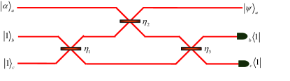
Figure 1: (Colour online) Schematic setup of the KLM circuit for generating a quantum state $\left|\psi_{a}\right\rangle$ from an inputting coherent state $\left|\alpha_{a}\right\rangle$ using three beam splitters (with reflection rates $\eta_{1},\eta_{2},\eta_{3}$ respectively), two single-photon sources, and two single-photon resolving detectors. In contrast with $\left|\alpha_{a}\right\rangle$, the generated state $\left|\psi_{a}\right\rangle$ has a wide range of nonclassical properties.

By tuning the parameters of the interaction, namely, $\left|\alpha\right|$, $\eta_{1}$, $\eta_{2}$, and $\eta_{3}$, the cofficients may be modulated, generating abroad class of nonclassical states with a wide range of nonclassical phenomena, as shown next by us.

II.3 Success probability of detection

Normalization is important for discussing the properties of a quantum state. The normalization factor of the generated states in theory is actually the probability $p_{d}$ of counting successfully single photons at the two auxiliary modes in experiment. The density operator of the generated state $\rho_{a}=\left|\psi_{a}\right\rangle\left\langle\psi_{a}\right|$ is expressed in Appendix C. According to $\mathrm{Tr}\left(\rho_{a}\right)=1$, the success probability to get the state $\left|\psi_{a}\right\rangle$ from our proposal is given by

$$p_{d} = (g_{0}+g_{1}\left|\alpha\right|^{2}+g_{2}\left|\alpha\right|^{4}$$ (4)

$$+g_{3}\left|\alpha\right|^{6}+g_{4}\left|\alpha\right|^{8})e^{-\left(1-S_{11}^{2}\right)\left|\alpha\right|^{2}},$$

Here $g_{0}$, $g_{1}$, $g_{2}$, $g_{3}$, and $g_{4}$ are given in appendix D.

In our following numerical works, the quantities under considering are discussed only in the two special cases: (1) set $\eta_{1}=\eta_{2}=\eta_{3}=\eta$ and change $\eta$, (2) set $\eta_{1}=\eta_{3}=1/2$ and change $\eta_{2}$. In order to exhibit numerically the probability $p_{d}$, we plot the contour of $p_{d}$ in the $\left(\eta,\left|\alpha\right|\right)$ plain space in Fig.2 (a) and in the $\left(\eta_{2},\left|\alpha\right|\right)$ plain space in Fig.2 (b). Additionally, we plot $p_{d}$ as a function of $\eta$ in Fig.2 (c) and as a function of $\eta_{2}$ in Fig.2 (d) for $\left|\alpha\right|=1,2,3$. For a large $\left|\alpha\right|$ and small $\eta$ (or $\eta_{2}$), the probability of detection $p_{d}$ is small and even less than $0.05$. For values closer to $\eta=1$, the generated state gets closer to the origin input state $\left|\alpha\right\rangle$ and the probability gets closer to $1$.

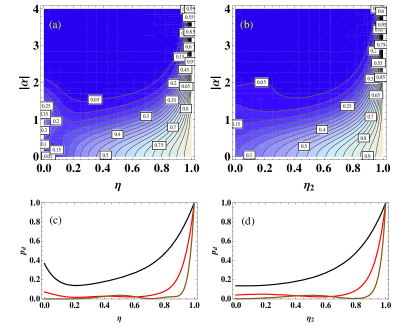
Figure 2: (Colour online) Success probability $p_{d}$ of detection (a) contour plot in ($\eta,\left|\alpha\right|$) space with $\eta=\eta_{1}=\eta_{2}=\eta_{3}$; (b) contour plot in ($\eta_{2},\left|\alpha\right|$) space with $\eta_{1}=\eta_{3}=1/2$; (c) as a fuction of $\eta$; (d) as a fuction of $\eta_{2}$. Here the black, red and brown lines are corresponding to $\left|\alpha\right|=1$, $\left|\alpha\right|=2$, $\left|\alpha\right|=3$, respectively. For a large amplitude of the coherent state $\left|\alpha\right|$, the probability is smaller than $0.05$. When $\eta$ is limit to $1$, the probability is limit to 1.

III Nonclassical properties of the generated states

Quantum states of light can be classified according to their statistical properties. They are usually compared to a reference state, namely, the coherent state 37 . In comparison with the input coherent state, what nonclassical properties will exhibit after meaurement induction in our proposed scheme. Analytical expressions of the expected values $\left\langle a^{{\dagger}k}a^{l}\right\rangle$ for arbitrary $k,l$ found in appendix F allow us to study the statistical properties of this generated states in our following works. Here, we will focus on studying some nonclassical properties of this generated quantum state, including anti-bunching effect and quadrature squeezing effect.

III.1 Anti-bunching effect

The second-order autocorrelation function $g^{\left(2\right)}\left(0\right)=\left\langle a^{\dagger 2}a^{2}\right\rangle/\left\langle a^{\dagger}a\right\rangle^{2}$ determines whether the source produce effects following antibunching ($g^{\left(2\right)}\left(0\right)<1$), bunching ($1\leqslant g^{\left(2\right)}\left(0\right)\leqslant 2$), or superbunching ($g^{\left(2\right)}\left(0\right)>2$). Additionally, it also determines whether the source produce photons following sub- ($g^{\left(2\right)}\left(0\right)<1$), super- ($g^{\left(2\right)}\left(0\right)>1$), or Poissonlike ($g^{\left(2\right)}\left(0\right)=1$) statistics 38 . For a coherent state, we have $g^{\left(2\right)}\left(0\right)=1$, which shows its character of Poisson distribution. Here, we shall examine the anti-bunching effect (a strictly nonclassical character) of the generated states, which describes whether the photons in the beam tend to stay apart.

The variations of $g^{\left(2\right)}\left(0\right)$ with the interaction parameters are showed in Fig.3. For several given amplitudes of coherent state ($\left|\alpha\right|=1,2,3$), we plot $g^{\left(2\right)}\left(0\right)$ as a function of $\eta$ in Fig.3 (a) and as a function of $\eta_{2}$ in Fig.3 (b). In a extreme case, we verify that $g^{\left(2\right)}\left(0\right)=1$ when $\eta$ (or $\eta_{2}$) is limit to $0$, i.e., the states corresponding to the input coherent state $\left|\alpha\right\rangle$. Moreover, the feasibility regions for antibunching, bunching and superbunching are exhibited in the ($\eta,\left|\alpha\right|$) parameter space in Fig.3 (c) and in the ($\eta_{2},\left|\alpha\right|$) parameter space in Fig.3 (d). It is found that there may present antibunching effect in a wide range of interaction parameters. The results show that the generated state $\left|\psi_{a}\right\rangle$ can exhibit a broad range of nonclassical features by tuning the interaction parameter.

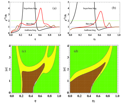
Figure 3: (Color online) Second-order autocorrelation function $g^{\left(2\right)}\left(0\right)$ of the generated state. The regions shows antibunching $g^{\left(2\right)}\left(0\right)<1$ (strictly nonclassical), bunching $1\leqslant g^{\left(2\right)}\left(0\right)\leqslant 2$, and superbunching $g^{\left(2\right)}\left(0\right)>2$. (a) as a function of $\eta$ ($\eta_{1}=\eta_{2}=\eta_{3}=\eta$); (b) as a function of $\eta_{2}$ ($\eta_{1}=\eta_{3}=1/2$). Here the black, red and brown lines are corresponding to $\left|\alpha\right|=1$, $\left|\alpha\right|=2$, $\left|\alpha\right|=3$, respectively. (c) the feasibility region in ($\eta$, $\left|\alpha\right|$) plain space.(d) the feasibility region in ($\eta_{2}$, $\left|\alpha\right|$) plain space. Here the blue, yellow and brown regions are corresponding to antibunching, bunching, and superbunching cases respectively.

III.2 Quadrature squeezing effect

Squeezed light has come a long way since its first demonstration 30 years 39 . Significant advancements have been made from the initial 0.3 dB squeezing till todys near 13 dB squeezing 40 . Hence we will ask two questions: (1) Whether our generated states are squeezed states? (2) If they are squeezed states, then how much can the squeezing degree be arrived? Here we will consider the squeezing effect of these states.

Firstly we make a brief review of quadrature squeezing effect. Many experiments have been carried out dealing with noise in the quadrature component of the field, which is defined by two quadrature operators $X=\left(a+a^{{\dagger}}\right)/\sqrt{2}$ and $P=\left(a-a^{{\dagger}}\right)/\left(\sqrt{2}i\right)$, analogous to the position and momentum of a harmonic oscillator 41 . Both quadrature variances, related with the creation and annhilation operators, can expressed as $\left\langle\Delta X^{2}\right\rangle=(\left\langle a^{{\dagger}2}\right\rangle-\left\langle a^{{\dagger}}\right\rangle^{2}+\left\langle a^{2}\right\rangle-\left\langle a\right\rangle^{2}+1)/2+\left\langle a^{{\dagger}}a\right\rangle-\left\langle a^{{\dagger}}\right\rangle\left\langle a\right\rangle$ and $\left\langle\Delta P^{2}\right\rangle=(-\left\langle a^{{\dagger}2}\right\rangle+\left\langle a^{{\dagger}}\right\rangle^{2}-\left\langle a^{2}\right\rangle+\left\langle a\right\rangle^{2}+1)/2+\left\langle a^{{\dagger}}a\right\rangle-\left\langle a^{{\dagger}}\right\rangle\left\langle a\right\rangle$ respectively, as can be seen from their definitions. These components cannot be measured simulatanously because of the commutation relation $[X,P]=i$. It follows that the product of the variances in the measurements of the two quadratures $X$ and $P$ satisfies $\Delta X^{2}\Delta P^{2}\geq 1/4$ (a Heisenberg inequality). For a vacuum state $\left|0\right\rangle$ or a coherent state $\left|\alpha\right\rangle$, the uncertainty relation is satisfied as an equality, and the two variances are identical: $\Delta X^{2}|_{\left|0\right\rangle,\left|\alpha\right\rangle}=\Delta P^{2}|_{\left|0\right\rangle,\left|\alpha\right\rangle}=1/2$. A quantum state is called squeezed if the variance of a quadrature amplitude is below the variance of a vacuum or a coherent state, i.e. $\Delta X^{2}<1/2$ or $\Delta P^{2}<1/2$. The squeezing effect of a light field comes at the expense of increasing the fluctuations in the other quadrature amplitude. Here we can adopt quantum squeezing quantified in a dB scale through $dB[X]=10\log_{10}\left(\Delta X^{2}/\Delta X^{2}|_{\left|0\right\rangle}\right)$, $dB[P]=10\log_{10}\left(\Delta P^{2}/\Delta P^{2}|_{\left|0\right\rangle}\right)$. In other words, if $dB[X]$ or $dB[P]$ is negative, this quantum state is a squeezed state.

In Fig.4 (a), the behaviour of $dB[X]$ as a function of $\eta$ ($=\eta_{1}=\eta_{2}=\eta_{3}$) for different $\left|\alpha\right|$. By minimizing the expression of $\Delta X^{2}$, the largest squeezing attained is around $0.321772$, below the vacuum noise level of $1/2$ by approximately $1.91422$ dB (using MATHENATICA) for $\left|\alpha\right|=1$. The squeezed degree is bigger than that ($1.25$ dB) in Ref.29 . In Fig.4 (b), the behaviour of $dB[X]$ as a function of $\eta_{2}$ for different $\left|\alpha\right|$ with $\eta_{1}=\eta_{3}=1/2$. Moreover, the purple regions show the feasibility squeezed region of $X$ quadrature component in the ($\eta,\left|\alpha\right|$) parameter space in Fig.4 (c) and in the ($\eta_{2},\left|\alpha\right|$) parameter space in Fig.4 (d). Fig.4 (c) and 4 (d) show a wide range of squeezing for $\left|\alpha\right|$ and $\eta\left(\eta_{2}\right)$.

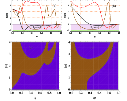
Figure 4: (Color online) Quadrature variance of $X$ component relative to the vacuum (unsqueezed) state in units of dB (a) as a function of $\eta$ ($\eta_{1}=\eta_{2}=\eta_{3}=\eta$); (b) as a function of $\eta_{2}$ ($\eta_{1}=\eta_{3}=1/2$). Here the black, red and brown solid lines are corresponding to $\left|\alpha\right|=1$, $\left|\alpha\right|=2$, $\left|\alpha\right|=3$ in X component, respectively. The feasibility squeezed (purple) and unsqueezed (brown) region of the $X$ component (c) in ($\eta$, $\left|\alpha\right|$) plain space; (d) in ($\eta_{2}$, $\left|\alpha\right|$) plain space.

IV Wigner function of the generated states

The negative Wigner function is a witness of the nonclassicality of a quantum state 42 . Additionaly, we can determinate whether this quantum state is non-Gaussian state from the form of the Wigner function 43 . Since non-Gaussian quantum state can provide quantum advantages not attainable classically, it is necessary to study the Wigner functions of our generated states.

The analytical expression of the Wigner function for the generated states is derived in appendix F. The results plotted in Fig.5 are obtained for optimal choices with different parameters $\left(\left|\alpha\right|,\eta_{1},\eta_{2},\eta_{3}\right)$. Fig.5 shows that the Wigner functions are negative in some regions of the phase space, which is a witness of the nonclassicality. As we all know, the coherent state is a typical Gaussian state whose Wigner function has no negative regions. In comparison with the input coherent state, the generated states show the non-Gaussian features with negative regions in moderate parameters range.

Meanwhile, we plot the negative volume $\delta$ as a function of $\eta$ (or $\eta_{2}$) for $\left|\alpha\right|=1$, $2$, $3$ in Fig.6. It is obvious to see that for different $\left|\alpha\right|$, the maximun negative volumn locate at different $\eta$ (or $\eta_{2}$). For instance, when $\left|\alpha\right|=1$, $\delta_{max}$ is located at $\eta=0$ (or $\eta_{2}=0$) and $\delta$ is decreaing with $\eta$ (or $\eta_{2}$) increasing and limit to zero at large $\eta$ (or $\eta_{2}$); For $\left|\alpha\right|=2$, $\delta_{max}$ is located at around $\eta=0.27$ (or $\eta_{2}=0.5$); For $\left|\alpha\right|=3$, $\delta_{max}$ is located at around $\eta=0.7$ (or $\eta_{2}=0.8$).

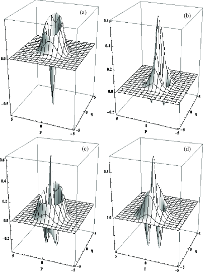
Figure 5: (Color online) Wigner functions of the measurement-induced state with parameters $\left(\left|\alpha\right|,\eta_{1},\eta_{2},\eta_{3}\right)$: (a) $\left(1,0.05,0.05,0.05\right)$; (b) $\left(2,0.5,0.05,0.5\right)$; (c) $\left(2,0.25,0.25,0.25\right)$; (d) $\left(2,0.5,0.5,0.5\right)$. The result shows that the Wigner function of the generated state has the negative regions, which is different from that of the input coherent state and also shows the nonclassical character.

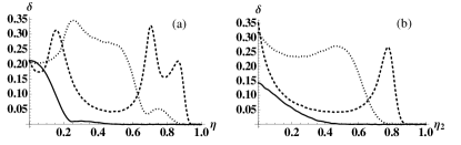
Figure 6: (Color online) The negative volumn $\delta$ of the Wigner functions of the generated states (a) as a function of $\eta$ ($\eta_{1}=\eta_{2}=\eta_{3}=\eta$); (b) as a function of $\eta_{2}$ ($\eta_{1}=\eta_{3}=1/2$). The solid, dotted and dashed line are corresponding to $\left|\alpha\right|=1$, $\left|\alpha\right|=2$, $\left|\alpha\right|=3$, respectively.

V Discussion and Conclusion

Our results show that there exist optimal nonclassical properites in different parameter ranges. The optimal performance as required can be obtained by adjusting the interaction parameters. A prominent character is that the the maxinum squeezing can be reached to $1.91422$ dB. In comparison with the states generated in Bartley’s work, the squeezing degree of our generated states is enhanced. In table I, we numerate some values of the probability of detection $p_{d}$, the auto-correlation function $g^{\left(2\right)}\left(0\right)$, the squeezing in $X$ component $dB[X]$, and the negative volume $\delta$ of the Wigner functions in their corresponding $\left(\left|\alpha\right|,\eta_{1},\eta_{2},\eta_{3}\right)$ parameters.

Table 1: Values of the probability of detection $p_{d}$, the auto-correlation function $g^{\left(2\right)}\left(0\right)$, the squeezing in $X$ component $dB[X]$, and the negative volume $\delta$ of the WFs in their corresponding interaction parameter values of $\left(\left|\alpha\right|,\eta_{1},\eta_{2},\eta_{3}\right)$.

$\left(\left|\alpha\right|,\eta_{1},\eta_{2},\eta_{3}\right)$	$p_{d}$	$g^{\left(2\right)}\left(0\right)$	$dB\left[X\right]$	$\delta$
$\left(1,0.3,0.3,0.3\right)$	0.15223	26.0347	-1.16685	0.0103
$\left(1,0.6,0.6,0.6\right)$	0.27011	0.43187	-0.52375	0.0010
$\left(1,0.9,0.9,0.9\right)$	0.67275	0.97122	-0.08971	0.0009
$\left(1,0.5,0.7,0.5\right)$	0.35303	0.76685	-0.31669	0.0009
$\left(2,0.5,0.7,0.5\right)$	0.03770	1.47059	-0.43680	0.0334
$\left(3,0.5,0.7,0.5\right)$	0.01392	0.99035	1.80934	0.1283

In summary, this paper employs two-fold quantum-optical catalysis to generate a class of nonclassical states based on KLM-type SU(3) interferometry. By measurement induction, we implemente a nonlinear operator $c_{0}+c_{1}a^{{\dagger}}+c_{2}a^{{\dagger}2}$ and obtain a broad class of useful non-Gaussian quantum states with higher nonclassicality. We discuss the success probability of detection and the nonclassical properties in terms of anti-bunching effect and squeezing effect as well as the negativity of the Wigner function. In compared with the input coherent state, these generated nonclassical states exhibit a lot of nonclassical properties. The results show that the optimal antibunching and the maximum squeezing as well as the maximum negative volume of the Wigner functions are located in different parameter points. Hence one can choose the optimal performance of these nonclassical properties to implement various technological tasks. In addition, the generation of these nonclassical states is feasible with current technology. The experiment realization of such states is desired to achieve in the future. Our results can provid a theoretical reference for experiments.

Appendix A: Transformation relation of the SU(3) interferometry

The network can be seen as three multiports in cascade, one for each of the beam splitters with the unitary operators $U_{j}\left(\eta_{j}\right)$ and the scattering matrices $S_{j}$ $\left(j=1,2,3\right)$. For each stage, the dyanamics is $U_{j}\left(a^{{\dagger}},b^{{\dagger}},c^{{\dagger}}\right)^{T}U_{j}^{{\dagger}}=S_{j}\left(a^{{\dagger}},b^{{\dagger}},c^{{\dagger}}\right)^{T}$, with the scattering metrix

$$S_{1}=\left(\begin{array}[]{ccc}1&0&0\\ 0&\sqrt{\eta_{1}}&\sqrt{1-\eta_{1}}\\ 0&\sqrt{1-\eta_{1}}&-\sqrt{\eta_{1}}\end{array}\right),$$

$$S_{2}=\left(\begin{array}[]{ccc}-\sqrt{\eta_{2}}&\sqrt{1-\eta_{2}}&0\\ \sqrt{1-\eta_{2}}&\sqrt{\eta_{2}}&0\\ 0&0&1\end{array}\right),$$

$$S_{3}=\left(\begin{array}[]{ccc}1&0&0\\ 0&\sqrt{\eta_{3}}&\sqrt{1-\eta_{3}}\\ 0&\sqrt{1-\eta_{3}}&-\sqrt{\eta_{3}}\end{array}\right),$$

So the total operator is $U=U_{3}\left(\eta_{3}\right)U_{2}\left(\eta_{2}\right)U_{1}\left(\eta_{1}\right)$ and the total scattering matrix is $S=S_{3}S_{2}S_{1}$. Thus Eq.(1) is obtained. One can also refer the detailed information in Ref.35 .

Appendix B: Explicit expression of the generated state

Substituting $\left|\alpha_{a}\right\rangle=e^{-\left|\alpha\right|^{2}/2+\alpha a^{{\dagger}}}\left|0_{a}\right\rangle$, $\left|1_{b}\right\rangle=\frac{d}{ds_{1}}e^{s_{1}b^{{\dagger}}}\left|0_{b}\right\rangle|_{s_{1}=0}$, $\left|1_{c}\right\rangle=\frac{d}{ds_{2}}e^{s_{2}c^{{\dagger}}}\left|0_{c}\right\rangle|_{s_{2}=0}$, $\left\langle 1_{b}\right|=\frac{d}{ds_{3}}\left\langle 0_{b}\right|e^{s_{3}b}|_{s_{3}=0}$ and $\left\langle 1_{c}\right|=\frac{d}{ds_{4}}\left\langle 0_{c}\right|e^{s_{4}c}|_{s_{4}=0}$, into Eq.(2) and using the transformation in Eq.(1) as well as the fact $U\left|0_{a}\right\rangle\left|0_{b}\right\rangle\left|0_{c}\right\rangle=\left|0_{a}\right\rangle\left|0_{b}\right\rangle\left|0_{c}\right\rangle$, we finally arrive at the derivative form of $\left|\psi_{a}\right\rangle$,

$$\left|\psi_{a}\right\rangle = \frac{e^{-\left|\alpha\right|^{2}/2}}{\sqrt{p_{d}}}\frac{d^{4}}{ds_{4}ds_{3}ds_{2}ds_{1}}e^{\alpha\left(S_{12}s_{3}+S_{13}s_{4}\right)}$$

$$\times e^{S_{22}s_{1}s_{3}+S_{23}s_{1}s_{4}+S_{32}s_{2}\allowbreak s_{3}+S_{33}s_{2}s_{4}}$$

$$\times e^{a^{{\dagger}}\left(\alpha S_{11}+S_{21}s_{1}+S_{31}s_{2}\right)}\left|0_{a}\right\rangle|_{s_{1}=s_{2}=s_{3}=s_{4}=0},$$

Therefore the explicit form in Eq.(2) can be obtained after making derivation.

Appendix C: Density operator of the generated state

The conjugate state of $\left|\psi_{a}\right\rangle$ can be given by

$$\left\langle\psi_{a}\right| = \frac{e^{-\left|\alpha\right|^{2}/2}}{\sqrt{p_{d}}}\frac{d^{4}}{dh_{4}dh_{3}dh_{2}dh_{1}}e^{\alpha^{\ast}\left(S_{12}h_{3}+S_{13}h_{4}\right)}$$

$$\times e^{S_{22}h_{1}h_{3}+S_{23}h_{1}h_{4}+S_{32}h_{2}\allowbreak h_{3}+S_{33}h_{2}h_{4}}$$

$$\times\left\langle 0_{a}\right|e^{a\left(\alpha^{\ast}S_{11}+S_{21}h_{1}+S_{31}h_{2}\right)}|_{h_{1}=h_{2}=h_{3}=h_{4}=0},$$

Then, the density operator is

$$\rho_{a} = \frac{e^{-\left|\alpha\right|^{2}}}{p_{d}}\frac{d^{8}}{dh_{4}dh_{3}dh_{2}dh_{1}ds_{4}ds_{3}ds_{2}ds_{1}}$$

$$\times e^{\alpha\left(S_{12}s_{3}+S_{13}s_{4}\right)+\alpha^{\ast}\left(S_{12}h_{3}+S_{13}h_{4}\right)}$$

$$\times e^{S_{22}s_{1}s_{3}+S_{23}s_{1}s_{4}+S_{32}s_{2}\allowbreak s_{3}+S_{33}s_{2}s_{4}}$$

$$\times e^{S_{22}h_{1}h_{3}+S_{23}h_{1}h_{4}+S_{32}h_{2}\allowbreak h_{3}+S_{33}h_{2}h_{4}}$$

$$\times e^{a^{{\dagger}}\left(\alpha S_{11}+S_{21}s_{1}+S_{31}s_{2}\right)}\left|0_{a}\right\rangle\left\langle 0_{a}\right|e^{a\left(\alpha^{\ast}S_{11}+S_{21}h_{1}+S_{31}h_{2}\right)}$$

$$|_{s_{1}=s_{2}=s_{3}=s_{4}=h_{1}=h_{2}=h_{3}=h_{4}=0}$$

Appendix D: Success probability $p_{d}$ of detection

Due to $\mathrm{tr}\left(\rho_{a}\right)=1$, we have

$$p_{d} = e^{-\left(1-S_{11}^{2}\right)\left|\alpha\right|^{2}}\frac{d^{8}}{dh_{4}dh_{3}dh_{2}dh_{1}ds_{4}ds_{3}ds_{2}ds_{1}}$$

$$\times e^{\left(S_{11}S_{21}\allowbreak h_{1}+S_{11}S_{31}h_{2}+S_{12}s_{3}+S_{13}s_{4}\right)\alpha}$$

$$\times e^{\left(S_{11}S_{21}s_{1}+S_{11}S_{31}s_{2}+S_{12}h_{3}+S_{13}h_{4}\right)\alpha^{\ast}}$$

$$\times e^{S_{22}\left(s_{1}s_{3}+h_{1}h_{3}\right)+S_{23}\left(s_{1}s_{4}+h_{1}h_{4}\right)+S_{21}^{2}s_{1}h_{1}+S_{31}^{2}s_{2}h_{2}}$$

$$\times e^{S_{32}\left(s_{2}\allowbreak s_{3}+h_{2}\allowbreak h_{3}\right)+S_{33}\left(s_{2}s_{4}+h_{2}h_{4}\right)+S_{21}S_{31}\left(s_{2}h_{1}+\allowbreak s_{1}h_{2}\right)}$$

$$|_{s_{1}=s_{2}=s_{3}=s_{4}=h_{1}=h_{2}=h_{3}=h_{4}=0}$$

which lead to the result in Eq.(4) with

$$g_{0}=\left(S_{23}S_{32}+S_{22}S_{33}\right)^{2},$$

$$g_{1} = (S_{13}S_{22}S_{31}+S_{12}S_{23}S_{31}+S_{13}S_{21}S_{32}+S_{12}S_{21}S_{33})$$

$$\times\left(S_{13}S_{22}S_{31}+S_{12}S_{23}S_{31}+S_{13}S_{21}S_{32}\right.$$

$$\left.+2S_{11}S_{23}S_{32}+S_{12}S_{21}S_{33}+2S_{11}S_{22}S_{33}\right),$$

$$g_{2} = S_{11}^{2}S_{13}^{2}\left(S_{22}S_{31}+S_{21}S_{32}\right)^{2}$$

$$+4S_{11}S_{12}^{2}S_{12}^{2}S_{13}S_{21}S_{31}\left(S_{23}S_{31}+S_{21}S_{33}\right)$$

$$+2S_{12}^{2}S_{13}^{2}S_{21}^{2}S_{31}^{2}+S_{11}^{2}S_{12}^{2}\left(S_{23}S_{31}+S_{21}S_{33}\right)^{2}$$

$$+4S_{11}S_{12}S_{13}S_{13}S_{21}S_{31}\left(S_{22}S_{31}+S_{21}S_{32}\right)$$

$$+2S_{11}^{2}S_{12}S_{13}S_{21}S_{32}\left(2S_{23}S_{31}+S_{21}S_{33}\right)$$

$$+2S_{11}^{2}S_{12}S_{13}S_{22}S_{31}\left(S_{23}S_{31}+2S_{21}S_{33}\right),$$

$$g_{3} = 2S_{11}^{3}S_{12}S_{13}^{2}S_{21}S_{31}\left(S_{22}S_{31}+S_{21}S_{32}\right)$$

$$+4S_{11}^{2}S_{12}^{2}S_{13}^{2}S_{21}^{2}S_{31}^{2}+2S_{11}^{3}S_{12}^{2}S_{13}^{2}S_{21}S_{31}S_{23}$$

$$+2S_{11}^{3}S_{12}^{2}S_{13}S_{21}^{2}S_{31}S_{33},$$

$$g_{4}=S_{11}^{4}S_{12}^{2}S_{13}^{2}S_{21}^{2}S_{31}^{2}.$$

Appendix E: General expressions of the expected values $\left\langle a^{{\dagger}k}a^{l}\right\rangle$

According to $\left\langle a^{{\dagger}k}a^{l}\right\rangle=\mathrm{tr}\left(a^{{\dagger}k}a^{l}\rho_{a}\right)$ and making detailed calculation, we obtain

$$\left\langle a^{{\dagger}k}a^{l}\right\rangle$$

$$= \frac{e^{-\left(1-S_{11}^{2}\right)\left|\alpha\right|^{2}}}{p_{d}}\frac{d^{8+k+l}}{dh_{4}dh_{3}dh_{2}dh_{1}ds_{4}ds_{3}ds_{2}ds_{1}d\mu^{k}d\nu^{l}}$$

$$\times e^{\left(S_{11}S_{21}h_{1}+S_{11}S_{31}h_{2}+S_{12}s_{3}+S_{13}s_{4}\right)\alpha}$$

$$\times e^{\left(S_{11}S_{21}s_{1}+\allowbreak S_{11}S_{31}s_{2}+S_{12}h_{3}+S_{13}h_{4}\right)\alpha^{\ast}}$$

$$\times e^{+S_{22}\left(s_{1}s_{3}+h_{1}h_{3}\right)+S_{23}\left(s_{1}s_{4}+h_{1}h_{4}\right)+S_{21}^{2}s_{1}h_{1}+S_{31}^{2}s_{2}h_{2}}$$

$$\times e^{+S_{32}\left(s_{2}\allowbreak s_{3}+h_{2}\allowbreak h_{3}\right)+S_{33}\left(s_{2}s_{4}+h_{2}h_{4}\right)+S_{21}\allowbreak S_{31}\left(s_{2}h_{1}+s_{1}h_{2}\right)}$$

$$\times e^{S_{11}\left(\mu\alpha^{\ast}+\nu\alpha\right)+\mu\left(S_{21}h_{1}+S_{31}h_{2}\right)+\nu\left(S_{21}\allowbreak s_{1}+S_{31}s_{2}\right)}$$

$$|_{s_{1}=s_{2}=s_{3}=s_{4}=h_{1}=h_{2}=h_{3}=h_{4}=\mu=\nu=0}.$$

Using this general expression, we can study the statistical properties of our generated states.

Appendix F: Wigner function of the generated state

According to the formula of the Wigner function in the coherent state representation $\left|z\right\rangle$, i.e $W(\beta)=\frac{2e^{2\left|\beta\right|^{2}}}{\pi}\int\frac{d^{2}z}{\pi}\left\langle-z\right|\rho\left|z\right\rangle e^{-2\left(z\beta^{\ast}-z^{\ast}\beta\right)}$ with $\beta=\left(q+ip\right)/\sqrt{2}$, the Wigner function is given by

$$W(\beta)$$

$$= \frac{2e^{-\left(1-S_{11}^{2}\right)\left|\alpha\right|^{2}-2\left|\beta-S_{11}\alpha\right|^{2}}}{\pi p_{d}}\frac{d^{8}}{dh_{4}dh_{3}dh_{2}dh_{1}ds_{4}ds_{3}ds_{2}ds_{1}}$$

$$\times e^{\alpha\left(-h_{1}S_{11}S_{21}-h_{2}S_{11}S_{31}+S_{12}s_{3}+S_{13}s_{4}\right)}$$

$$\times e^{\alpha^{\ast}\left(-S_{11}S_{21}s_{1}\allowbreak-S_{11}S_{31}s_{2}+S_{12}h_{3}+S_{13}h_{4}\right)}$$

$$\times e^{+S_{22}\left(s_{1}s_{3}+h_{1}h_{3}\right)+S_{23}\left(s_{1}s_{4}+h_{1}h_{4}\right)-S_{21}^{2}s_{1}h_{1}-S_{31}^{2}s_{2}h_{2}}$$

$$\times e^{+S_{32}\left(s_{2}\allowbreak s_{3}+h_{2}\allowbreak h_{3}\right)+S_{33}\left(s_{2}s_{4}+h_{2}h_{4}\right)-S_{21}S_{31}\left(s_{2}h_{1}+s_{1}h_{2}\right)}$$

$$\times e^{2\beta\left(h_{1}S_{21}+h_{2}S_{31}\right)+2\beta^{\ast}\left(S_{21}s_{1}+S_{31}\allowbreak s_{2}\right)}$$

$$|_{s_{1}=s_{2}=s_{3}=s_{4}=h_{1}=h_{2}=h_{3}=h_{4}=0}.$$

After derivative, the analytical expression can be obtained.

References

• (1) S. L. Braunstein and P. van Loock, Rev. Mod. Phys. 77, 5130 (2005).
• (2) P. Kok and B. W. Lovett, Introduction to Optical Quantum Information Processing (Cambridge University Press, New York, 2010).
• (3) S. L Braunstein and H. J. Kimble, Phys. Rev. Lett. 80, 869 (1998).
• (4) G. J. Milburn and Samuel L. Braunstein, Phys. Rev. A 60, 937 (1999).
• (5) P. M. Anisimov, G. M. Raterman, A. Chiruvelli, W. N. Plick, S. D. Huver, H. Lee, and J. P. Dowling, Phys. Rev. Lett. 104, 103602 (2010).
• (6) S. Lloyd and S.L Braunstein, Phys. Rev. Lett. 82, 1784 (1999).
• (7) P. C. Humphrey, W. S. Kolthammer, J. Nunn, M. Barbieri, A. Datta, and I. A. Walmsley, Phys. Rev. Lett. 113, 130502 (2014).
• (8) V. V. Dodonov and V. I. Man’ko, Theory of Nonclassical States of light (Taylor & Francis Inc., New York, 2003).
• (9) G. S. Agarwal and K. Tara, Phys. Rev. A 43, 492 (1991).
• (10) A. Zavatta, S. Viciani, and M. Bellini, Science 306, 660 (2004).
• (11) A. Zavatta, V. Parigi, and M. Bellini, Phys. Rev. A 75, 052106 (2007).
• (12) X. B. Wang, T. Hiroshima, A. Tomita, and M. Hayashi, Phys. Rep. 448, 1 (2007).
• (13) C. Weedbrook, S. Pirandola, R. Garcia-Patron, N. J. Cerf, T. C. Ralph, J. H. Shapiro, and S. Lloyd, Rev. Mod. Phys. 84, 621 (2012).
• (14) J. Eisert, S. Scheel, and M. B. Plenio, Phys. Rev. Lett. 89, 137903 (2002).
• (15) J. Eisert, D. E. Browne, S. Scheel, and M. B. Plenio, Ann. Phys. 311, 431 (2004).
• (16) J. Niset, J. Fiurasek, and N. J. Cerf, Phys. Rev. Lett. 102, 120501 (2009).
• (17) M. Hillery, R. F. O’Connell, M. O. Scully, and E. P. Wigner, Phys. Rep. 106, 121 (1984).
• (18) A. Kowalewska-Kudłaszyk, W. Leoński, and Jan Peřina, Jr., Phys. Rev. A 83, 052326 (2011).
• (19) S. D. Barlett and B. C. Sanders. Phys. Rev. A 65, 042304 (2002).
• (20) Y. R. Shen, The Principles of Nonlinear optics (Wiley, New York, 1984).
• (21) D. E. Browne, J. Eisert, S. Scheel, and M. B. Plenio, Phys. Rev. A 67, 062320 (2003).
• (22) J. Eisert, Phys. Rev. Lett. 95, 040502 (2005).
• (23) P. Kok, W. J. Munro, K. Nemoto, T. C. Ralph, J. P. Dowling, and G. J. Milburn, Rev. Mod. Phys. 79, 135 (2007).
• (24) A. Kitagawa, M. Takeoka, K. Wakui, and M. Sasaki, Phys. Rev. A 72, 022334 (2005).
• (25) S. Y. Lee and H. Nha, Phys. Rev. A 82, 053812 (2010).
• (26) S. Y. Lee and H. Nha, Phys. Rev. A 85, 043816 (2012).
• (27) M. Dakna, T. Anhut, T. Opatrny, L. Knoll, and D. G. Welsch, Phys. Rev. A 55, 3184 (1997).
• (28) A. I. Lvovsky and J. Mlynek, Phys. Rev. Lett. 88, 250401 (2002)
• (29) T. J. Bartley, G. Donati, J. B. Spring, X. M. Jin, M. Barbieri, A. Datta, B. J. Smith, and I. A. Walmsley, Phys. Rev. A 86, 043820 (2012)
• (30) X. X. Xu, Phys. Rev. A 92, 012318 (2015).
• (31) E. Knill, R. Laflamme, and G.J. Milburn, Nature, 409, 46 (2001).
• (32) T. C. Ralph, A. G. White, W. J. Munro, and G. J. Milburn, Phys. Rev. A 65, 012314 (2001).
• (33) S. Scheel, K. Nemoto, W. J. Munro, and P. L. Knight, Phys. Rev. A 68, 032310 (2003).
• (34) M. Reck, A. Zeilinger, H. J. Bernstein, and P. Bertani, Phys. Rev. Lett. 73, 58 (1994).
• (35) J. Skaar, J. C. G. Escartin, and H. Landro, Am. J. Phys. 72, 1385 (2004).
• (36) J. Carolan, et al., Science, 349, 711 (2015).
• (37) S. M. Barnett and P. M. Radmore, Methods in Theoretical Quantum Optics (Clarendon Press, Oxford, 1997).
• (38) L. Davidovich, Rev. Mod. Phys. 68, 127 (1996).
• (39) R. Slusher, L. Hollberg, B. Yurke, J. Mertz, and J. Valley, Phys. Rev. Lett. 55, 2409 (1985).
• (40) U. L. Anderson, T. Gehring, C. Marquardt, and G. Leuchs, arXiv: 1511.03250 (2015).
• (41) D. F. Walls and G. J. Miburn, Quantum Optics (Springer-Verlag Berlin Heidelberg, New York, 1994).
• (42) R. Filip, Phys. Rev. A 87, 042308 (2013).
• (43) K. E. Cahill and R. J. Glauber, Phys. Rev. 177, 1882 (1969).