Evaluating Morphological Computation in Muscle and DC-motor Driven Models of Human Hopping

Abstract

In the context of embodied artificial intelligence, morphological computation refers to processes which are conducted by the body (and environment) that otherwise would have to be performed by the brain. Exploiting environmental and morphological properties is an important feature of embodied systems. The main reason is that it allows to significantly reduce the controller complexity. An important aspect of morphological computation is that it cannot be assigned to an embodied system per se, but that it is, as we show, behavior- and state-dependent. In this work, we evaluate two different measures of morphological computation that can be applied in robotic systems and in computer simulations of biological movement. As an example, these measures were evaluated on muscle and DC-motor driven hopping models. We show that a state-dependent analysis of the hopping behaviors provides additional insights that cannot be gained from the averaged measures alone. This work includes algorithms and computer code for the measures.

1 Introduction

Morphological computation (MC), in the context of embodied (artificial) intelligence, refers to processes which are conducted by the body (and environment) that otherwise would have to be performed by the brain [11]. A nice example of MC is given by Wootton [18] (see p. 188), who describes how “active muscular forces cannot entirely control the wing shape in flight. They can only interact dynamically with the aerodynamic and inertial forces that the wings experience and with the wing’s own elasticity; the instantaneous results of these interactions are essentially determined by the architecture of the wing itself […]”

MC is relevant in the study of biological and robotic systems. In robotics, a quantification of MC can be used e.g. as part of a reward function in a reinforcement learning setting to encourage the outsourcing of computation to the morphology, thereby enabling complex behaviors that result from comparably simple controllers. The relationship of embodiment and controller complexity has been recently studied in [10]. MC measures can also be used to evaluate the robot’s morphology during the design process. For biological systems, energy efficiency is important and an evolutionary advantage. Exploiting the embodiment can lead to more energy efficient behaviors, and hence, MC may be a driving force in evolution.

In biological systems, movements are typically generated by muscles. Several simulation studies have shown that the muscles’ typical non-linear contraction dynamics can be exploited in movement generation with very simple control strategies [14]. Muscles improve movement stability in comparison to torque driven models [16] or simplified linearized muscle models (for an overview see [5]). Muscles also reduce the influence of the controller on the actual kinematics (they can act as a low-pass filter). This means that the hopping kinematics of the system is more pre-determined with non-linear muscle characteristics than with simplified linear muscle characteristics [5]. And finally, in hopping movements, muscles reduce the control effort (amount of information required to control the movement) by a factor of approximately 20 in comparison to a DC-motor driven movement [7].

In view of these results we expect that MC plays an important role in the control of muscle driven movement. To study this quantitatively, a suitable measure for MC is required. There are several approaches to formalize MC [8, 13, 12]. In our previous work we have focused on an agent-centric perspective of measuring MC [19] and we have applied an information decomposition of the sensorimotor loop to measure and better understand MC [4]. Both publications used a binary toy world model to evaluate the measures. With this toy model, it was possible to show that these measures capture the conceptual idea of MC and, in consequence, that they are candidates to measure MC in more complex and more realistic systems.

The goal of this publication is to evaluate two measures of MC on biologically realistic hopping models. With this, we want to demonstrate their applicability in non-trivial, realistic scenarios. Based on our previous findings (see above), we hypothesize that MC is higher in hopping movements driven by a non-linear muscle compared to those driven by a simplified linear muscle or a DC-motor, for the following reason. Our experiments show that a state-dependent analysis of MC for the different models leads to insights, which cannot be gained from the averaged measures alone.

Furthermore, we provide detailed instructions, including MATLAB^® code, on how to apply these measures to robotic systems and to computer simulations. With this, we hope to provide a tool for the evaluation of MC in a large variety of applications.

The quantifications of MC require a formal representation of the sensorimotor loop (see Fig. 1), which is introduced in the next section as far as it is required to understand the remainder of this work. For further information, the reader is referred to [9, 20, 19, 2].

2 The Sensorimotor Loop

The conceptual idea of the sensorimotor loop is similar to the basic control loop systematics, which is the basis of robotics and also of computer simulations of human movement. In our understanding, a cognitive system consists of a brain or controller, which sends signals to the system’s actuators, thereby affecting the system’s environment. We prefer to capture the body and environment in a single random variable named world. This is consistent with other concepts of agent-environment distinctions. An example for such a distinction can be found in the context of reinforcement learning, where the environment (world) is everything that cannot be changed arbitrarily by the agent [15]. A more thorough discussion of the brain-body-environment distinction can be found in [17, 1] and a more recent discussion can be found in [3]. A brief example of a world, based on a robot simulation, is given below. The loop is closed as the system acquires information about its internal state (e.g. current pose) and its world through its sensors.

For simplicity, we only discuss the sensorimotor loop for reactive systems. This is plausible, because behaviors which exploit the embodiment (e.g. walking, swimming, flying) are typically reactive. This leaves us with three (stochastic) processes $S(t)$, $A(t)$, and $W(t)$, $t\in\mathbb{N},$ that constitute the sensorimotor loop (see Fig. 1), which take values $s$, $a$, and $w$, in the sensor, actuator, and world state spaces (their respective domains will be clear from the context). The directed edges (see Fig. 1) reflect causal dependencies between these random variables. We consider time to be discrete, i.e., $t\in\mathbb{N}$ and are interested in what happens in a single time step. Therefore, we use the following notation. Random variables without any time index refer to some fixed time $t$ and primed variables to time $t+1$, i.e., the two variables $S$, $S^{\prime}$ refer to $S(t)$ and $S(t+1)$.

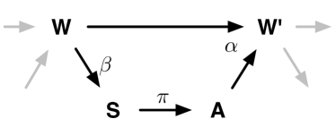
Figure 1: Causal model of the sensorimotor loop. This figure depicts a single step of an embodied, reactive system’s sensorimotor loop. A detailed explanation is given in Sec. 2

Starting with the initial distribution over world states, denoted by $p(w)$, the sensorimotor loop for reactive systems is given by three conditional probability distributions, $\beta$, $\alpha$, $\pi$, also referred to as kernels. The sensor kernel, which determines how the agent perceives the world, is denoted by $\beta(s|w)$, the agent’s controller or policy is denoted by $\pi(a|s)$, and finally, the world dynamics kernel is denoted by $\alpha(w^{\prime}|w,a)$.

To understand the function of the world dynamics kernel $\alpha(w^{\prime}|w,a)$ it is useful to think of a robotic simulation. In this scenario, the world state $W$ is the state of the simulator at a given time step, which includes the pose of all objects, their velocities, applied forces, etc. The actuator state $A$ is the value that the controller passes on to the physics engine prior to the next physics update. Hence, the world dynamics kernel $\alpha(w^{\prime}|w,a)$ is closely related to the forward model that is known in the context of robotics and biomechanics.

Based on this notation, we can now formulate quantifications of MC in the next section.

3 Quantifying Morphological Computation

In the introduction, we stated that MC relates to the computation that the body (and environment) performs that otherwise would have to be conducted by the controller (or brain). This means that we want to measure the extent to which the system’s behavior is the result of the world dynamics (i.e., the body’s internal dynamics and it’s interaction with its world) and how much of the behavior is determined by the policy $\pi$ (see Fig. 1).

In our previous publication [19] we have defined two concepts to quantify MC, from which the two measures below are taken and derived.

3.1 Morphological computation as conditional mutual information ($\mathrm{MC}_{\mathrm{W}}$)

The first quantification, that is used in this work, was introduced in [19]. The idea behind it can be summarized in the following way. The world dynamics kernel $\alpha(w^{\prime}|w,a)$ captures the influence of the actuator signal $A$ and the previous world state $W$ on the next world state $W^{\prime}$. A complete lack of MC would mean that the behavior of the system is entirely determined by the system’s controller, and hence, by the actuator state $A$. In this case, the world dynamics kernel reduces to $p(w^{\prime}|a)$. Every difference from this assumption means that the previous world state $W$ had an influence, and hence, information about $W$ changes the distribution over the next world states $W^{\prime}$. The discrepancy of these two distributions can be measured with the average of the Kullback-Leibler divergence $D_{\mathrm{KL}}(\alpha(w^{\prime}|w,a)||p(w^{\prime}|a))$, which is also known as the conditional mutual information $I(W^{\prime};W|A)$. This distance is formally given by (see also Alg. 2 in App. 8)

$$\mathrm{MC}_{\mathrm{W}}:=\sum_{w^{\prime},w,a}p(w^{\prime},w,a)\log_{2}\frac{\alpha(w^{\prime}|w,a)}{p(w^{\prime}|a)}.$$

3.2 Morphological computation as comparison of behavior and controller complexity ($\mathrm{MC}_{\mathrm{MI}}$)

The second quantification follows concept one of [19]. The assumption that underlies this concept is that, for a given behavior, MC decreases with an increasing effect of the action $A$ on the next world state $W^{\prime}$. The corresponding measure $\mathrm{MC}_{\mathrm{A}}\propto-I(W^{\prime};A|W)$ cannot be used in systems with deterministic policy, because for these systems $I(W^{\prime};A|W)=0$ (see App. 9). Therefore, for this publication, we require an adaptation that operates on world states and is applicable to deterministic systems.

The new measure compares the complexity of the behavior with the complexity of the controller. The complexity of the behavior can be measured by the mutual information of consecutive world states, $I(W^{\prime};W)$, and the complexity of the controller can be measured by the mutual information of sensor and actuator states, $I(A;S)$, for the following reason. The mutual information of two random variables can also be written as difference of entropies:

$$I(X;Y) =H(X)-H(X|Y)$$

$$H(X) =-\sum_{x}p(x)\log_{2}p(x)$$

$$H(X|Y) =-\sum_{x,y}p(x,y)\log_{2}p(x|y),$$

which, applied to our setting, means that the mutual information $I(W^{\prime};W)$ is high, if we have a high entropy over world states $W^{\prime}$ (first term) that are highly predicable (second term). Summarized, this means that the mutual information $I(W^{\prime};W)$ is high if the system shows a diverse but non-random behavior. Obviously, this is what we would like to see in an embodied system. On the other hand, a system with high MC should produce a complex behavior based on a controller with low complexity. Hence, we want to reduce the mutual information $I(A;S)$, because this either means that the policy has a low diversity in its output (low entropy over actuator states $H(A)$) or that there is only a very low correlation between sensor states $S$ and actuator states $A$ (high conditional entropy $H(A|S)$). Therefore, we define the second measure as the difference of these two terms, which is (see also Alg. 4 in Sec. 8)

$$\mathrm{MC}_{\mathrm{MI}}=I(W^{\prime};W)-I(A;S).$$

For deterministic systems, as those studied in this work, the two measures are closely related. In particular, it holds that $\mathrm{MC}_{\mathrm{W}}-\mathrm{MC}_{\mathrm{MI}}=H(A|W^{\prime})$ (see App. 10). The inequality $\mathrm{MC}_{\mathrm{W}}\geq\mathrm{MC}_{\mathrm{MI}}$ may not be satisfied always, because discretization can introduce stochasticity.

Note that in the case of a passive observer, i.e., a system that observes the world but in which there is no causal dependency between the action and the next world state (i.e., missing connection between $A$ and $W^{\prime}$ in Fig. 1), the controller complexity $I(A;S)$ in Eq. (2) will reduce the amount of MC measured by $\mathrm{MC}_{\mathrm{MI}}$, although the actuator state does not influence the world dynamics. This might be perceived as a potential shortcoming. In the context discussed in this paper, e.g. data recorded from biological or robotic systems, we think that this will not be an issue.

The next section introduces the hopping models on which the two measures are evaluated.

4 Hopping models

In a reduced model, hopping motions can be described by a one-dimensional differential equation [6]:

$$m\ddot{y}=-mg+\begin{cases}0&y>l_{0}\text{\,\,\,\,\,\ flight phase}\\ F_{\text{L}}&y\leq l_{0}\text{\,\,\,\,\,\ ground contact}\end{cases}\,\,\,,$$

where the point mass $m=80\,\mathrm{kg}$ represents the total mass of the hopper which is accelerated by the gravitational force ($g=-9.81\,\mathrm{m/s^{2}}$) in negative $y$-direction. An opposing leg force $F_{\text{L}}$ in positive $y$-direction can act only during ground contact ($y\leq l_{0}=1\,\mathrm{m}$). Hopping motions are then characterized by alternating flight and stance phases. For this manuscript, we investigated three different models for the leg force. All models have in common, that the leg force depends on a control signal $u(t)$ and the system state $y(t)$, $\dot{y}(t)$: $F_{\text{L}}=F_{\text{L}}(u(t),y(t),\dot{y}(t))$, meaning, that the force modulation partially depends on the controller output $u(t)$ and partially on the dynamic characteristics, or material properties of the actuator. The control parameters of all three models were adjusted to generate the same periodic hopping height of $\max(y(t))=1.070\,\mathrm{m}$. All models were implemented in MATLAB^® Simulink^™ (Ver2014b) and solved with ode45 Dormand-Prince solver with absolute and relative tolerances of $10^{-12}$. The models were solved and integrated in time for $T=8\,\mathrm{s}$ and model output was generated at $1\,\mathrm{kHz}$ sampling frequency.

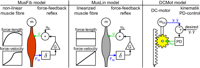
Figure 2: Hopping models. The MusFib model considers the non-linear contraction dynamics of active muscle fibers and is driven by a mono-synaptic force-feedback reflex. The MusLin model only differs in the contraction dynamics, where the force-length relation is neglected and the force-velocity relation is approximated linearly. The DCMot model generates the leg force with a DC-motor. It is controlled by a proportional-differential controller (PD), enforcing the desired trajectory. The desired trajectory is the recorded trajectory from the MusFib Model. The sensor signals are shown as blue arrows, the actuator control signals are shown as green arrows. In case of the muscle models, the sensor signal is the muscle force $F_{M}$ and the actuator control signal is the neural muscle stimulation $u$. In case of the DC-motor model, the sensor signals are the position and velocity of the mass, and the actuator control signal is the motor armature voltage $u_{DC}$.

4.1 Muscle-Fiber model (MusFib)

A biological muscle generates its active force in muscle fibers whose contraction dynamics are well studied. It was found that the contraction dynamics are qualitatively and quantitatively (with some normalizations) very similar across muscles of all sizes and across many species. In the MusFib model, the leg force is modeled to incorporate the active muscle fibers’ contraction dynamics. The model has been motivated and described in detail elsewhere [6, 5, 7]. In a nutshell, the material properties of the muscle fibers are characterized by two terms modulating the leg force

$$F_{L,\text{MusFib}}=a(t)F_{\text{fib}}(l_{M},\dot{l}_{M}).$$

The first term $a(t)$ represents the muscle activity. The activity depends on the neural stimulation of the muscle $0.001\leq u(t)\leq 1$ and is governed by biochemical processes modeled as a first-order ODE called activation dynamics

$$\dot{a}=\frac{1}{\tau}\left(u-a\right),$$

with the time constant $\tau=10\,\mathrm{ms}$. The second term in Eq. (4) $F_{\text{fib}}$ considers the force-length and force-velocity relation of biological muscle fibers. It is a function of the system state, i.e., the muscle length $l_{M}=y$ and muscle contraction velocity $\dot{l}_{M}=\dot{y}$ during ground contact $y\leq l_{0}$ and constant $l_{M}=l_{0}$ $\dot{l}_{M}=0$ during flight $y>l_{0}$:

$$F_{\text{fib}}=\begin{aligned} &F_{\max}\cdot\exp\left(-c\left\lvert\frac{l_{M}-l_{\text{opt}}}{l_{\text{opt}}w}\right\lvert^{3}\right)\\ &\times\begin{cases}\frac{\dot{l}_{M,\text{max}}+\dot{l}_{M}}{\dot{l}_{M,\text{max}}-K\dot{l}_{M}}&\dot{l}_{M}>0\\ N+(N-1)\frac{\dot{l}_{M,\text{max}}-\dot{l}_{M}}{-7.56K\dot{l}_{M}-\dot{l}_{M,\text{max}}}&\dot{l}_{M}\leq 0\end{cases}\,\,\,.\end{aligned}$$

Here we use a maximum isometric muscle force $F_{\text{max}}=2.5\,\mathrm{kN}$, an optimal muscle length $l_{\text{opt}}=0.9\,\mathrm{m}$, force-length parameters $w=0.45\,\mathrm{m}$ and $c=30$, and force-velocity parameters $\dot{l}_{\max}=-3.5\,\mathrm{ms^{-1}}$, $K=1.5$, and $N=1.5$ [6].

In this model, periodic hopping is generated with a controller representing a mono-synaptic force-feedback. The neural muscle stimulation

$$u(t)=G\cdot F_{L,\text{MusFib}}(t-\delta)+u_{0}$$

is based on the time delayed ($\delta=15\,\mathrm{ms}$) muscle fiber force $F_{L,\text{MusFib}}$. The feedback gain is $G=2.4/F_{\max}$ and the stimulation at touch down $u_{0}=0.027$.

This model neither considers leg geometry nor tendon elasticity and is therefore the simplest hopping model with muscle-fiber-like contraction dynamics. The model output was the world state $w(t)=(y(t),\dot{y}(t),\ddot{y}(t))$, the sensor state $s(t)=F_{L\text{,MusFib}}(t)$, and the actuator control command $a(t)=u(t)$. For this model, these are the values that the random variables $W$, $S$, and $A$ take at each time step.

4.2 Linearized Muscle-Fiber model (MusLin)

This model differs from the model MusFib only in the representation of the force-length-velocity relation, i.e., $F_{L,\text{MusLin}}=a(t)F_{\text{lin}}(\dot{l}_{M})$ (see Eq. (6)). More precisely, the force-length relation is neglected and the force-velocity relation is approximated linearly

$$F_{\text{lin}}=1\cdot(1-\mu\dot{l}_{M}),$$

with $\mu=0.25\,\mathrm{m/s}$. Feedback gain $G=0.8/F_{\max}$ and stimulation at touch down $u_{0}=0.19$ were chosen to achieve the same hopping height as the MusFib model.

4.3 DC-Motor model (DCMot)

An approach to mimic biological movement in a technical system (robot) is to track recorded kinematic trajectories with electric motors and a PD-control approach. The DCMot model implements this approach (slightly modified from [7]). The leg force generated by the DC-motor was modeled as

$$F_{L,\text{DCMot}}=\gamma T_{DC}=\gamma k_{T}I_{DC},$$

where $k_{T}=0.126\,\mathrm{Nm/A}$ is the motor constant, $I_{DC}$ the current through the motor windings, $\gamma=100:1$ the ratio of an ideal gear translating the rotational torque $T_{DC}$ and movement $\dot{\varphi}(t)=\gamma\dot{y}(t)$ of the motor to the translational leg force and movement required for hopping. The electrical characteristics of the motor can be modeled as

$$\dot{I}_{DC}=\frac{1}{L}\left(u_{DC}-k_{T}\gamma\dot{y}(t)-RI_{DC}\right),$$

where $-48\,\mathrm{V}\leq u_{DC}\leq 48\,\mathrm{V}$ is the armature voltage (control signal), $R=7.19\,\mathrm{\Omega}$ the resistance, and $L=1.6\,\mathrm{mH}$ the inductance of the motor windings. The motor parameters were taken from a commercially available DC-motor commonly used in robotics applications (Maxon EC-max 40, nominal Torque $T_{\text{nominal}}=0.212\,\mathrm{Nm}$). As this relatively small motor would not be able to lift the same mass, the body mass was adapted to guarantee comparable accelerations

$$m_{DC}=\frac{\gamma T_{\text{nominal}}}{F_{\max}}m=0.68\,\mathrm{kg}.$$

The recorded kinematic trajectory $y_{\text{rec}}(t)$ and $\dot{y}_{\text{rec}}(t)$ during ground contact was taken from the periodic hopping trajectory of the MusFib model. This trajectory was enforced with a PD-controller

$$u_{DC}(t)=K_{P}(y_{\text{rec}}(t)-y(t))+K_{D}(\dot{y}_{\text{rec}}(t)-\dot{y}(t))$$

with feedback gains $K_{P}=5000\,\mathrm{V/m}$ and $K_{D}=500\,\mathrm{Vs/m}$.

This model is the simplest implementation of negative feedback control that allows to enforce a desired hopping trajectory on a technical system. The model output was the world state $w(t)=(y(t),\dot{y}(t),\ddot{y}(t))$, the sensor state $s(t)=(y(t),\dot{y}(t))$, and the actuator control command $a(t)=u_{DC}(t)$.

5 Experiments

This section discusses the experiments that were conducted with the hopping models and the preprocessing of the data. Algorithms for the calculations are provided in the appendix (Sec. 8) and implemented MATLAB^® code can be downloaded from http://github.com/kzahedi/MC/ (commit c332c18, 30. Nov. 2015). A C++ implementation is available at http://github.com/kzahedi/entropy/.

At this stage, the measures operate on discrete state spaces (see Eqs. (1)–(3) and Algs. 2-4). Hence, the data was discretised in the following way. To ensure the comparability of the results, the domain (range of values) for each variable (e.g. the position $y$) was calculated over all hopping models. Then, the data of each variable was discretised into 300 values (bins). The algorithm for the discretisation is described in Alg. 1. Different binning resolutions were evaluated and the most stable results were found for more than 100 bins. Finding the optimal binning resolution is a problem of itself and beyond the scope of this work. In practice, however, a reasonable binning can be found by increasing the binning until further increase has little influence on the outcome of the measures.

The possible range of actuator values are different for the motor and muscle models. For the muscle models, the values are in the unit interval, i.e., $a(t)\in[0,1]$, whereas the values for the motor can have higher values (see above). Hence, to ensure comparability, we normalized the actions of the motor to the unit interval before they were discretized.

The hopping models are deterministic, which means that only a few hopping cycles are necessary to estimate the required probability distributions. To ensure comparability of the results, we parameterized the hopping models to achieve the same hopping height.

6 RESULTS

Tab. 1 shows the value of the two MC measures for the three hopping models.

	MusFib	MusLin	DCMot
$\mathrm{MC}_{\mathrm{W}}$	7.219 bits	4.975 bits	4.960 bits
$\mathrm{MC}_{\mathrm{MI}}$	7.310 bits	5.153 bits	4.990 bits

Table 1: Numerical results on the hopping models for $\mathrm{MC}_{\mathrm{W}}$ (see Eq. (1)) and $\mathrm{MC}_{\mathrm{MI}}$ (see Eq. (2)).

Compared to the MusFib model, the two other models result in significantly lower measurement of MC ($\approx 30\%$ less). This result complements previous findings showing that the minimum information required to generate hopping is reduced by the material properties of the non-linear muscle fibers compared to the DC-motor driven model [7].

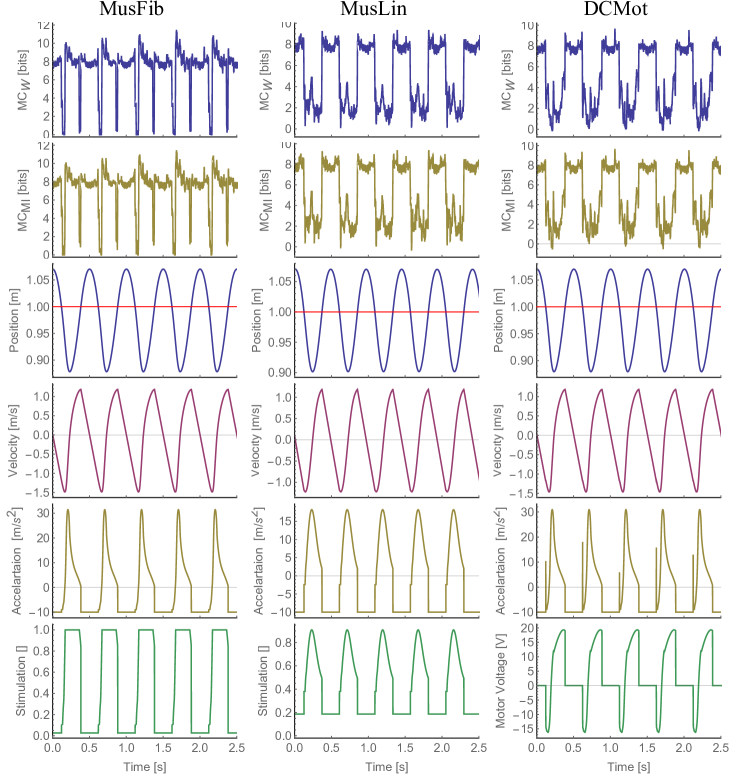
Figure 4: Plots of state-dependent MC (first two rows) and the world state (following four rows) for all muscle models. The red line in the position plot indicates the time steps at which the hopper touches ground (position is below the red line).

This also confirms previous findings that the non-linear contraction dynamics reduces the influence of the controller on the actual hopping kinematics in comparison to a linearized muscle model [6, 5]. To better understand the differences of the models, we plotted the state-dependent MC (see Alg. 3). Fig. 3 shows the values of $\mathrm{MC}_{\mathrm{W}}$ for each state of the models during two hopping cycles. We chose to discuss $\mathrm{MC}_{\mathrm{W}}$ only, because the plots of $\mathrm{MC}_{\mathrm{W}}$ and $\mathrm{MC}_{\mathrm{MI}}$ are very similar, and hence, a discussion of the state-dependent $\mathrm{MC}_{\mathrm{MI}}$ will not provide any additional insights. The plots for all models and the entire data are shown in Fig. 4.

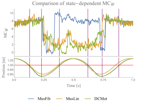
Figure 3: Comparison of state-dependent MC for $\mathrm{MC}_{\mathrm{W}}$ on the three hopping models. The lower plots in each Figure visualize the hopping position (out of proportion for better visibility). The red line indicates stance and flight phases. The full data is shown in Fig. 4. The plots only show a small fraction of the recorded data. For better readability, all the plots for MC are smoothened with a moving average of block size 5.

The orange line shows the state-dependent MC for the linear muscle model (MusLin), and finally, the blue line shows the values for the non-linear muscle model (MusFib). The green line shows the state-dependent MC for the motor model (DCMot). In the figure, the lower lines show the position $y$ of the center of mass over time. The DCMot model is parameterized to follow the trajectory of the MusFib model (see Eq. (12)), which is why the blue and green position plots coincide. The original data is shown in Fig. 4. There are basically three phases, which need to be distinguished (indicated by the vertical lines). First, the flight phase, during which the hopper does not touch the ground (position plots are above the red line), second, the deceleration phase, which occurs after landing (position is below the red line but still declining), and finally, the acceleration phase, in which the position is below the red line but increasing.

The first observation is that MC is equal for all models during most of the flight phase (position above the red line) and that it seems to be proportional to the velocity of the systems. During flight, the behavior of the system is governed only by the interaction of the body (mass, velocity) and the environment (gravity) and not by the actuator models. This explains why the values coincide for the three models.

For all models, MC drops as soon as the systems touch the ground. DCMot and MusLin reach their highest values only during the flight phase, which can be expected at least from a motor model that is not designed to exploit MC. The graphs also reveal that the MusLin model shows slightly higher MC around mid-stance phase, compared to the DCMot model. For the non-linear muscle model, the behavior is different. Shortly after touching the ground, the system shows a strong decline of MC, which is followed by a strong incline during the deceleration with the muscle. Contrary to the other two models, the non-linear muscle model MusFib shows the highest values when the muscle is contracted the most (until mid-stance). This is an interesting result, as it shows that the non-linear muscle is capable of showing more MC while the muscle is operating, compared to the flight phase, in which the behavior is only determined by the interaction of the body and environment.

7 CONCLUSIONS

This work presented two different quantifications of MC including algorithms and MATLAB^® code to use them. We demonstrated their applicability in experiments with non-trivial, biologically realistic hopping models and discussed the importance of a state-based analysis of morphological computation. The first quantification, $\mathrm{MC}_{\mathrm{W}}$, measures MC as the conditional mutual information of the world and actuator states. Morphological computation is the additional information that the previous world state $W$ provides about the next world state $W^{\prime}$, given that the current actuator state $A$ is known. The second quantification, $\mathrm{MC}_{\mathrm{MI}}$, compares the behavior and controller complexity to determine the amount of MC.

The numerical results of the two quantifications confirm our hypothesis that the MusFib model should show significantly higher MC, compared to the two other models (MusLin, DCMot). We also showed that a state-dependent analysis of MC leads to additional insights. Here we see that the non-linear muscle model is capable of showing significantly more morphological computation in the stance phase, compared to the flight phase, during which the behavior is only determined by the interaction of the body and environment. This shows that morphological computation is not only behavior-, but also state-dependent. Future work will include the analysis of additional behaviors, such as walking and running, for which we expect, based on the findings of this work, to see a more morphological computation of the non-linear muscle model MusFib.

APPENDIX

8 Algorithms

This section presents the algorithms in pseudo-code. The MATLAB^® code that was used for this publication can be downloaded from http://github.com/kzahedi/MC/ (commit c332c18, 30. Nov. 2015). A C++ implementation is available at http://github.com/kzahedi/entropy/.

Note that we use a compressed notion in Alg. 2–5, in which $x^{\prime}=x(t+1)$ and $x=x(t)$.

0:  $t=1,2,\ldots,T$

0:  time series $y=(y(t))$, $\dot{y}=(\dot{y}(t))$, $\ddot{y}=(\ddot{y}(t))$, $a=(a(t))$, $s=(s(t))$, $t=1,2,\ldots,T$

0:  Number of bins $B_{x}$ for time series $x$

1:  $y^{*}(t)=(y(t)-\mathrm{min}(y))/(\mathrm{max}(y)-\mathrm{min}(y)))\cdot B_{y}$

2:  repeat previous step analogously for $\dot{y}$, $\ddot{y}$, $a$, and $s$ to generate discretised time series $\dot{y}^{*}$, $\ddot{y}^{*}$, $a^{*}$, and $s^{*}$

3:  $w^{*}(t)=y^{*}(t)+B_{y}\cdot\dot{y}^{*}(t)+B_{y}B_{\dot{y}}\cdot\ddot{y}^{*}(t)$

4:  The previous step must be applied to sensors and actuators, if they result from more than one time series

5:  $w^{\prime*}=(w^{*}(2),w^{*}(3),\ldots,w^{*}(T))$

6:  $w^{*}=(w^{*}(1),w^{*}(2),\ldots,w^{*}(T-1))$

7:  $s^{*}=(s^{*}(1),s^{*}(2),\ldots,s^{*}(T-1))$

8:  $a^{*}=(a^{*}(1),a^{*}(2),\ldots,a^{*}(T-1))$

Algorithm 1 Discretisation of the data. This part is the same for all measures, depending on which time series are required. The $\mathrm{min}$ and $\mathrm{max}$ were determined of the data of all hopping models.

1:  $p(w^{\prime},w,a)\leftarrow(0)_{|W|\times|W|\times|A|}$ {Matrix with $|W|\times|W|\times|A|$ entries set to zero}

2:  for $t=1,2,\ldots,T-1$ and $w_{t+1},w_{t}\in w^{*},a_{t}\in a^{*}$ do

3:     $p(w_{t+1},w_{t},a_{t})\leftarrow p(w_{t+1},w_{t},a_{t})+1$

4:  end for

5:  $p(w^{\prime},w,a)\leftarrow p(w^{\prime},w,a)/(T-1)$

6:  Estimate $p(w^{\prime},a)$ from $w^{*},a^{*}$ or by summing over $w$

7:  $p(w^{\prime}|w,a)=\nicefrac{{p(w^{\prime},w,a)}}{{\sum_{w^{\prime}}p(w^{\prime},w,a)}}$

8:  $p(w^{\prime}|a)=\nicefrac{{p(w^{\prime},a)}}{{\sum_{w^{\prime}}p(w^{\prime},a)}}$

9:  $\mathrm{MC}_{\mathrm{W}}=\sum_{w^{\prime},w,a}p(w^{\prime},w,a)\log_{2}\frac{p(w^{\prime}|w,a)}{p(w^{\prime}|a)}$

Algorithm 2 Algorithm for $\mathrm{MC}_{\mathrm{W}}$.

1:  Perform steps 1–8 from Alg. 2

2:  for $t=1,2,\ldots,T-1$ and $w^{\prime},w\in w^{*},a\in a^{*}$ do

3:     $\mathrm{MC}_{\mathrm{W}}(t)=\log_{2}\frac{p(w^{\prime}|w,a)}{p(w^{\prime}|a)}$

4:  end for

Algorithm 3 Algorithm for state-dependent $\mathrm{MC}_{\mathrm{W}}(t)$.

1:  Estimate $p(w^{\prime},w)$ from $w^{*}$ (see Alg. 2)

2:  Estimate $p(a,s)$ from $a^{*},s^{*}$, (see Alg. 2)

3:  $H(W^{\prime})=-\sum_{w^{\prime}}p(w^{\prime})\log_{2}p(w^{\prime})$

4:  $H(W^{\prime}|W)=-\sum_{w^{\prime},w}p(w^{\prime},w)\log_{2}\nicefrac{{p(w^{\prime},w)}}{{\sum_{w^{\prime}}p(w^{\prime},w)}}$

5:  $H(A)=-\sum_{a}p(a)\log_{2}p(a)$

6:  $H(A|S)=-\sum_{a,s}p(a,s)\log_{2}\nicefrac{{p(a,s)}}{{\sum_{a}p(a,s)}}$

7:  $\mathrm{MC}_{\mathrm{MI}}=H(W^{\prime})-H(W^{\prime}|W)-H(A)+H(A|S)$

Algorithm 4 Algorithm for $\mathrm{MC}_{\mathrm{MI}}$.

1:  Perform step 1–2 from Alg. 4

2:  for $t=1,2,\ldots,T-1$ and $w^{\prime},w\in w^{*},a\in a^{*},s\in s^{*}$ do

3:     $\mathrm{MC}_{\mathrm{MI}}(t)=\begin{aligned} &\log_{2}p(w^{\prime})-\log_{2}p(w^{\prime}|w)\\ &+\log_{2}p(a)-\log_{2}p(a|s)\end{aligned}$

4:  end for

Algorithm 5 Algorithm for state-dependent $\mathrm{MC}_{\mathrm{MI}}(t)$.

9 $I(W^{\prime};A|W)=0$ for deterministic systems

In the case where $\alpha(w^{\prime}|w,a)$, $\beta(s|w)$, and $\pi(a|s)$ are deterministic, the conditional entropy $H(W^{\prime}|W)$ vanishes. It follows that

$$0\leq I(W^{\prime};A|W) =H(W^{\prime}|W)-H(W^{\prime}|W,A)$$

$$\leq H(W^{\prime}|W)$$

$$=0.$$

10 Relation between $\mathrm{MC}_{\mathrm{W}}$and $\mathrm{MC}_{\mathrm{MI}}$

From the following equality

$$I(W^{\prime};W,A) =I(W^{\prime};W)+I(W^{\prime};A|W)$$

$$=I(W^{\prime};A)+I(W^{\prime};W|A)$$

we can derive

$$\underbrace{I(W^{\prime};W|A)}_{\mathrm{MC}_{\mathrm{W}}} =\underbrace{I(W^{\prime};W)-I(A;S)}_{\mathrm{MC}_{\mathrm{MI}}}+I(A;S)$$

$$+I(W^{\prime};A|W)-I(W^{\prime};A)$$

$$\mathrm{MC}_{\mathrm{W}}-\mathrm{MC}_{\mathrm{MI}} =I(A;S)+I(W^{\prime};A|W)-I(W^{\prime};A)$$

$$=H(A)-H(A|S)$$

$$\phantom{=}+H(W^{\prime}|W)-H(W^{\prime}|W,A)$$

$$\phantom{=}-H(A)+H(A|W^{\prime})$$

$$=H(A|W^{\prime})$$

For deterministic systems the conditional entropies $H(A|S)=H(W^{\prime}|W)=H(W^{\prime}|A,W)=0$. We show this exemplarily for $H(A|S)$. If the action $A$ is a function of the sensor state $S$, then $p(a,s)=p(a|s)$ is either one or zero, because there is exactly one actuator value for every sensor state. Hence, $H(A|S)=\sum_{a,s}p(a,s)\log p(a|s)=0$. The equality $\mathrm{MC}_{\mathrm{MI}}-\mathrm{MC}_{\mathrm{W}}=H(A|W^{\prime})$ is not hold in Tab. 1, because the discretization introduces stochasticity, and hence, the conditional entropies are only approximately zero, i.e., $H(A|S)\approx H(W^{\prime}|W)\approx H(W^{\prime}|A,W)\approx 0$

References

- [1] N. Ay and W. Löhr. The umwelt of an embodied agent — a measure-theoretic definition. Theory in Biosciences, to appear.
- [2] N. Ay and K. Zahedi. An information theoretic approach to intention and deliberative decision-making of embodied systems. In Advances in cognitive neurodynamics III. Springer, Heidelberg, 2013.
- [3] A. Clark. Being There: Putting Brain, Body, and World Together Again. MIT Press, Cambridge, MA, USA, 1996.
- [4] K. Ghazi-Zahedi and J. Rauh. Quantifying morphological computation based on an information decomposition of the sensorimotor loop. In Proceedings of the 13th European Conference on Artificial Life (ECAL 2015), pages 70—77, July 2015.
- [5] D. F. B. Haeufle, S. Grimmer, K.-T. Kalveram, and A. Seyfarth. Integration of intrinsic muscle properties, feed-forward and feedback signals for generating and stabilizing hopping. Journal of the Royal Society Interface, 9(72):1458–1469, 07 2012.
- [6] D. F. B. Haeufle, S. Grimmer, and A. Seyfarth. The role of intrinsic muscle properties for stable hopping—stability is achieved by the force–velocity relation. Bioinspiration & Biomimetics, 5(1):016004, 2010.
- [7] D. F. B. Haeufle, M. Günther, G. Wunner, and S. Schmitt. Quantifying control effort of biological and technical movements: An information-entropy-based approach. Phys. Rev. E, 89:012716, Jan 2014.
- [8] H. Hauser, A. Ijspeert, R. M. Füchslin, R. Pfeifer, and W. Maass. Towards a theoretical foundation for morphological computation with compliant bodies. Biological Cybernetics, 105(5-6):355–370, 2011.
- [9] A. S. Klyubin, D. Polani, and C. L. Nehaniv. Organization of the information flow in the perception-action loop of evolved agents. In Evolvable Hardware, 2004. Proceedings. 2004 NASA/DoD Conference on, pages 177–180, 2004.
- [10] G. Montúfar, K. Ghazi-Zahedi, and N. Ay. A theory of cheap control in embodied systems. PLoS Comput Biol, 11(9):e1004427, 09 2015.
- [11] R. Pfeifer and J. C. Bongard. How the Body Shapes the Way We Think: A New View of Intelligence. The MIT Press (Bradford Books), Cambridge, MA, 2006.
- [12] D. Polani. An informational perspective on how the embodiment can relieve cognitive burden. In Artificial Life (ALIFE), 2011 IEEE Symposium on, pages 78–85, April 2011.
- [13] E. A. Rückert and G. Neumann. Stochastic optimal control methods for investigating the power of morphological computation. Artificial Life, 19(1):115–131, 2013.
- [14] S. Schmitt and D. F. B. Haeufle. Mechanics and Thermodynamics of Biological Muscle - A Simple Model Approach. In Alexander Verl, Alin Albu-Schäffer, Oliver Brock, and Annika Raatz, editors, Soft Robotics, pages 134–144. Springer, 1 edition, 2015.
- [15] R. S. Sutton and A. G. Barto. Reinforcement Learning: An Introduction. MIT Press, 1998.
- [16] A. J. van Soest and M. F. Bobbert. The contribution of muscle properties in the control of explosive movements. Biological Cybernetics, 69(3):195–204, jul 1993.
- [17] J. von Uexkuell. A stroll through the worlds of animals and men. In C. H. Schiller, editor, Instinctive Behavior, pages 5–80. International Universities Press, New York, 1957 [1934].
- [18] R. J. Wootton. Functional morphology of insect wings. Annual Review of Entomology, 37(1):113–140, 2012/01/06 1992.
- [19] K. Zahedi and N. Ay. Quantifying morphological computation. Entropy, 15(5):1887–1915, 2013.
- [20] K. Zahedi, N. Ay, and R. Der. Higher coordination with less control – a result of information maximization in the sensori-motor loop. Adaptive Behavior, 18(3–4):338–355, 2010.