Decay law and time dilatation

Abstract

We study the decay law for a moving unstable particle. The usual time-dilatation formula states that the decay width for an unstable state moving with a momentum $p$ and mass $M$ is $\tilde{\Gamma}_{p}=\Gamma M/\sqrt{p^{2}+M^{2}}$ with $\Gamma$ being the decay width in the rest frame. In agreement with previous studies, we show that in the context of QM as well as QFT this equation is not correct provided that the quantum measurement is performed in a reference frame in which the unstable particle has momentum $p$ (note, a momentum eigenstate is not a velocity eigenstate in QM). We then give, to our knowledge for the first time, an analytic expression of an improved formula and we show that the deviation from $\tilde{\Gamma}_{p}$ has a maximum for $p/M=\sqrt{2/3},$ but is typically very small. Then, the result can be easily generalized to a momentum wave packet and also to an arbitrary initial state. Here, we give a very general expression of the non-decay probability. As a next step, we show that care is needed when one makes a boost of an unstable state with zero momentum/velocity: namely, the resulting state has zero overlap with the elements of the basis of unstable states (it is already decayed!). However, when considering a spread in velocity, one finds again that $\tilde{\Gamma}_{p}$ is typically a very good approximation. The study of a velocity wave-packet represents an interesting subject which constitutes one of the main outcomes of the present manuscript. In the end, it should be stressed that there is no whatsoever breaking of special relativity, but as usual in QM, one should specify which kind of measurement on which kind of state is performed.

1 Introduction

Time dilatation is one of the most striking and beautiful consequences of special (and also general) relativity. It is experimentally precisely verified, yet it still fascinates us because it is so much different from our common sense: it shows the inexistence of a ‘present’ for all the observers and it generates many ‘paradoxes’, such as the renowned twins’ one. Its formulation is now parts of textbooks. Two observes, Alice (A) and Bob (B), move away from each other with constant velocity $v$. The relation among the coordinates of Bob and Alice is given by a Lorentz transformation. Alice has a clock (of whatever type!) in her hands. The clock makes a ‘click’ after a certain time $T$ which links the events $(0,0)$ and $(T,0)$ in her reference frame. Then, the time interval between the two events as measured by Bob is $\gamma T$ with $\gamma=1/\sqrt{1-v^{2}}.$ This is the usual time dilatation.

Another fascinating – and in a certain sense even more astonishing– part of modern physics is Quantum Mechanics (QM), in which randomness plays a central role: when a measurement is performed, the wave function of a quantum state instantaneously collapses to one of the eigenstates of the measured observable. An unstable quantum state, such as an unstable elementary particle, is one of the best examples to show the features of QM: the state of the system is a superposition of decayed and undecayed, and –upon measurement through an appropriate apparatus– a collapse to either decayed or not decayed takes place. Indeed, Schrödinger [1] had chosen the decay of a radioactive atom to trigger his sadistic but fortunately only ideal cat-killing machine, in such a way to put also the state of the cat into a superposition of alive and dead (unless, of course, the cat itself is regarded as a measuring device). The merging of special relativity and QM is Quantum Field Theory (QFT), which is the correct theoretical framework to describe to creation and annihilation of particles and thus -in ultimate analysis- to describe decays.

Now, Alice can use unstable particles as a clock. She prepares at $t=0$ a box of $N_{0}$ unstable states which have zero velocity, i.e. they are all at rest with Alice. She performs measurements and finds that the number of states decreases as $N(t)=N_{0}P_{nd}(t),$ where $P_{nd}(t)$ is the nondecay probability as measured by Alice. In the exponential limit [2, 3]:

$$P_{nd}(t)=e^{-\Gamma t}\text{ , }\tau=\Gamma^{-1}\text{ `lifetime'.}$$ (1)

It is now theoretically [4, 5, 6, 7, 8, 9, 10, 11] and experimentally [12, 13] established that deviations from the exponential decay exist, but they are usually small. We shall consider at first this limit in our numerical examples, but we will also present general expressions which naturally take into account departures from the exponential decay.

Now, what about Bob? The usual answer is that Bob ‘sees’ the unstable particles living longer. This is because of time dilatation. Thus, Bob should ‘see’ an increased lifetime of $\tau_{B}=\gamma\tau>\tau.$ In other words, the decay width as measured by Bob is given by the standard “Einstein” formula:

$$\frac{\Gamma}{\gamma}\equiv\frac{\Gamma M}{\sqrt{p^{2}+M^{2}}}=\tilde{\Gamma}_{p}\text{ ,}$$ (2)

where $M$ is the rest mass of the unstable particle. This is indeed the usual explanation behind the famous expression ‘the long lifetime of the muons’. Namely, the muons produced in the atmosphere manage to reach detectors located on the earth because of time dilatation: they move fast enough so that, in the earth reference frame, the decay width is sizably smaller and the decay time larger (see also the direct experimental verification in Ref. [14]). But what does it mean to ‘see’? We need to be precise in this respect.

Namely, it is important to stress from the very beginning the following point: if Alice performs the decayed/undecayed measurement in her reference frame, then Bob confirms the formula (2) exactly. The question here is slightly but crucially different: what does it happen if the detector is in the rest frame of Bob, who performs the decayed/undecayed measurement? In other words, is there a difference if it is Alice or Bob who is making the experiment?

We study the problem in four different steps. First (Sec. 2) we consider the case in which the unstable state has a definite momentum $p$ w.r.t. the measuring device. Here, we review previous existing works on the subject [17, 18, 19, 20, 21, 22, 23, 24, 25]: the general outcome is that Eq. (2) does not hold for such a system, even if it is a very good approximation. Moreover, we also present an analytical formula for the decay width $\Gamma_{p}$ in the Breit-Wigner limit. At the same time, we quantify the deviations in Fig. 1 and give further analytic expressions for the deviations from Eq. (2). In this context, it is important to stress that in QM and QFT an unstable state with definite momentum does not have a definite velocity, thus this situation does not correspond to a boost but rather to a momentum translation of a zero-velocity unstable state. Then, strictly speaking, this is not what Bob would measure, but it represents a very well defined theoretical setup (for instance, for a “momentum translated” observer Charlie).

The second step (Sec. 3) is the generalization to a momentum wave packet. Here a subtle but very important point concerns the definition of the basis of unstable states: we shall argue that the nondecay probability of a generic state $\left|\Psi\right\rangle$ is not the survival probability $\left|\left\langle\Psi\left|e^{-iHt}\right|\Psi\right\rangle\right|^{2}$, but that one should project onto a suitable basis. We also argue that the only consistent choice of such a basis is to use the set of unstable states with definite momentum (which can be obtained from the zero-velocity unstable state by momentum translations). Then, in the end of this section we also study the non-decay probability for a fully arbitrary initial state, leading to the most general result of the present paper.

As a third step (Sec. 4) we study -by using the formalism developed in Sec. 3- a boost of a zero-velocity unstable state and thus obtain an eigenstate of velocity (this is what Bob would measure). Quite surprisingly, the boosted state is already decayed: the boosted muon consists -for Bob and for his measuring apparatus- of an electron and two neutrinos; a boosted pion consists of two photons, and so on and so fort. This result is in agreement with Ref. [23], where it was called ‘decay caused by boost’. In this respect, Eq. (2) is completely wrong. In this section we also discuss the survival probability of a state with definite velocity, which -as presented in Refs. [23, 26, 21]- shows a quite amusing Lorentz contraction of time instead of dilation. This problem does not arise if the definition of Sec. 3 concerning the decayed/undecayed assessment is used.

The result of Sec. 4 is however very ‘delicate’ as we describe in the fourth and last step (Sec. 5): it is strictly valid only if we perform a boost on a state which have exactly zero momentum (or velocity). If a more realistic velocity wave-packet is considered, we find again that the decay law is well approximated by Eq. (2). Namely, using again Sec. 3, there is a nonzero overlap with the set of undecayed states as soon as a velocity spreading is implemented. The results, which are depicted in Fig. 2, constitute one of the main contributions of the present paper. Finally, we summarize the manuscript in Sec. 6.

2 Decay law of a state with definite momentum

We consider a spacial one-dimensional system described by the Hamiltonian $H$, whose eigenstates are denoted as

$$\left|m,p\right\rangle=U_{p}\left|m,0\right\rangle\text{ ,}$$

where $U_{p}$ is the unitary operator associated to the translation in momentum space. The state $\left|m,p\right\rangle$ has definite energy, $H\left|m,p\right\rangle=\sqrt{p^{2}+m^{2}}\left|m,p\right\rangle$, definite momentum, $P\left|m,p\right\rangle=p\left|m,p\right\rangle,$ as well as a definite velocity: $\left(P/H\right)\left|m,p\right\rangle=\left(p/\gamma m\right)\left|m,p\right\rangle.$ The normalization is given by: $\left\langle m_{1},p_{1}|m_{2},p_{2}\right\rangle=\delta(m_{1}-m_{2})\delta(p_{1}-p_{2}).$

An unstable state with definite momentum $p$ is denoted as $\left|S,p\right\rangle=U_{p}$ $\left|S,0\right\rangle$:

$$\left|S,p\right\rangle=\int_{0}^{\infty}\mathrm{dm}a_{S}(m)\left|m,p\right\rangle\text{ .}$$ (3)

The quantity $d_{S}(m)=\left|a_{S}(m)\right|^{2}$ is the mass distribution: $d_{S}(m)dm$ is the probability that the unstable particle $S$ has a mass between $m$ and $m+dm.$ As a consequence, $\int_{0}^{\infty}dmd_{S}(m)=1$. The normalization $\left\langle S,p_{1}|S,p_{2}\right\rangle=\delta(p_{1}-p_{2})$ follows. Note, Eq. (3) is not an state with definite velocity. This is due to the fact that each state $\left|m,p\right\rangle$ in the superposition has a different velocity $p/\left(\gamma m\right)$. The theory of decays is discussed in great detail for the case $p=0$ in Refs. [7, 15, 16] and Refs. therein. Moreover, as shown in Ref. [11], QFT at the one-loop resummed level can be also described within such formalism. Thus, our discussions includes from the very beginning not only QM but also QFT.

A very useful, although not exact, approximation both in QM and in QFT is the Breit-Wigner (BW) formula, $d_{S}^{BW}(m)=\frac{\Gamma}{2\pi}\left[(m-M)^{2}+\Gamma^{2}/4\right]^{-1}$. By starting from a properly normalized state with zero momentum, $\left|S,0\right\rangle/\sqrt{\delta(p=0)}$ and upon extending the integral to negative masses (this is strictly speaking unphysical, but the induced error is very small if the ratio $\Gamma/M\ll 1$) we obtain the amplitude

$$a(t,0)=\frac{1}{\delta(p=0)}\left\langle S,0\left|e^{-iHt}\right|S,0\right\rangle\simeq\int_{-\infty}^{\infty}\mathrm{dm}d_{S}^{BW}(m)e^{-imt}=e^{-iMt-\Gamma t/2}\text{ ,}$$ (4)

ergo the survival probability of the state $\left|S\right\rangle$ is $P_{nd}(t)=\left|a(t,0)\right|^{2}=e^{-\Gamma t}$, which is the usual decay law already introduced in Eq. (1).

As mentioned in the Introduction, it is now well known that deviations from the exponential decay exist. They stem from the fact that any realistic distribution $d_{S}(m)$ should be zero below a certain energy threshold $m_{0}\geq 0$, thus the integral in the r.h.s. of Eq. (4) should extend from $m_{0}$ upward (e.g., in a two-body decay the threshold energy is given by the sum of the rest masses produced in the decay, see also Ref. [20] for the study of the useful case $m_{0}=0$). Moreover, $d_{S}(m)$ should also fall down faster than $1/m^{2}$ for large $m$ due to form factors [7]. Both properties lead to long-time and short-time deviations from the exponential decay law $P_{nd}(t)=\left|a(t,0)\right|^{2}=e^{-\Gamma t},$ respectively. Yet, these deviations are usually small and occur in a very short time interval at the beginning of the decay and at a very late decay times (typically, of the order of $10\Gamma^{-1}$). Thus, there is a long time interval in which the exponential decay is very well realized. In this work, we aim to concentrate on the study of decays in relation with special relativity. Thus, in the present paper, we shall limit our numerical investigations to the Breit-Wigner limit. The reason is that, as we shall see, there are -even in this limit- interesting aspects which need further investigations and clarifications. Yet, general expressions valid beyond the Breit-Wigner limit are presented in the next section.

We now turn to the calculation of the non-decay probability of a state with definite but non vanishing momentum and present a derivation similar to the works of Refs. [18, 19, 20, 21, 22, 23, 24, 25]. To this end, we consider a (normalized) state $\left|S,p\right\rangle/\sqrt{\delta(p=0)}$ with a generic momentum $p,$ we find the following non-decay amplitude:

$$a(t,p) =\frac{1}{\delta(p=0)}\left\langle S,p\left|e^{-iHt}\right|S,p\right\rangle=\int_{-\infty}^{\infty}\mathrm{dm}d_{S}(m)e^{-i\sqrt{m^{2}+p^{2}}t}$$

$$\simeq\int_{-\infty}^{\infty}\mathrm{dm}d_{S}^{BW}(m)e^{-i\sqrt{m^{2}+p^{2}}t}=e^{-i\sqrt{(M-i\Gamma/2)^{2}+p^{2}}t}\text{ .}$$ (5)

For the investigation of similar equations we refer also to Refs. [20, 22, 25]. In the BW-limit, the non-decay (survival) probability reads

$$P_{nd}(t)=\left|a(t,p)\right|^{2}=e^{-\Gamma_{p}t}$$ (6)

with

$$\Gamma_{p}=2\operatorname{Im}\left[\sqrt{(M-i\Gamma/2)^{2}+p^{2}}\right]\text{ .}$$ (7)

Quite interesting, $\Gamma_{p}$ can be recasted in the analytic expression:

$$\Gamma_{p}=\sqrt{2}\sqrt{\left[\left(M^{2}-\frac{\Gamma^{2}}{4}+p^{2}\right)^{2}+M^{2}\Gamma^{2}\right]^{1/2}-\left(M^{2}-\frac{\Gamma^{2}}{4}+p^{2}\right)}\text{ .}$$ (8)

One realizes that $\Gamma_{p}$ differs from the standard formula of Eq. (2): $\Gamma_{p}\neq\tilde{\Gamma}_{p}=\Gamma M/\sqrt{p^{2}+M^{2}}$. Deviations where already discussed in Refs. [17, 18, 19, 20, 21, 22, 23, 24, 25]. We thus confirm those results and present -to our knowledge for the first time- the analytic expression (8) for the decay width of an unstable particle with definite momentum $p$. One can indeed easily proof that for $\Gamma/M\ll 1$ one reobtains, as expected, that $\Gamma_{p}\simeq\tilde{\Gamma}_{p}$. Notice that, while our Eq. (8) is only valid in the (typically very good) exponential limit, we feel that it is always useful to have -whenever possible- an analytic expression, especially in the context of connecting Quantum Mechanics and Special Relativity.

As a next point, it is natural to ask how good Eq. (2) is. For small $\Gamma/M$, the difference

$$\Delta=\frac{\Gamma_{p}-\tilde{\Gamma}_{p}}{M}$$ (9)

has a maximum for

$$\frac{p_{\max}}{M}=\sqrt{\frac{2}{3}}\simeq 0.816\text{ .}$$ (10)

The value of the difference at the maximum scales as:

$$\Delta_{\max}=\frac{\Gamma_{p_{\max}}-\tilde{\Gamma}_{p_{\max}}}{M}\simeq\frac{3}{100}\sqrt{\frac{3}{5}}\left(\frac{\Gamma}{M}\right)^{3}\text{ .}$$ (11)

As an example, in Fig. 1 we plot $\Delta$ as function of $p/M$ for the numerical choice $\Gamma/M=1/100$.

Eq. (2) turns out to be an extremely good approximation. For instance, in the case of the muon ($M=105.6583$ MeV, $\Gamma=2.99\cdot 10^{-16}$ MeV), we get an astonishingly small deviation: $\Gamma_{p_{\max}}-\tilde{\Gamma}_{p_{\max}}\simeq 5.598\cdot 10^{-53}$ MeV. The deviation increases only very slightly with increasing decay width. For the neutral pion ($M=134.9766$ MeV, $\Gamma=7.72\cdot 10^{-6}$ MeV) we get $\Gamma_{p_{\max}}-\tilde{\Gamma}_{p_{\max}}\simeq 5.81\cdot 10^{-22}$ MeV. Only for strong decays the deviations become somewhat larger. For the $\rho$ meson, ($M=775.26$ MeV, $\Gamma=147.8$ MeV) we get $\Gamma_{p_{\max}}-\tilde{\Gamma}_{p_{\max}}\simeq 0.125$ MeV (all numerical values are from Ref. [27]).

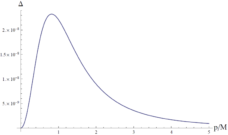
Figure 1: Difference between our result of Eq. (8) and the standard formula of Eq. (2) as function of $p$ for the ratio $\Gamma/M=1/100.$ The position of the minimum $p_{\max}/M=\sqrt{2/3}$ is constant for decreasing $\Gamma/M.$ The height of the maximum scales as given in Eq. (11), thus the deviation decreases very fast for decreasing $\Gamma/M.$

A direct experimental verification of this deviation seems at present difficult because of the very small departure (a very high precision is required, much beyond the one in Ref. [14]). However, it is a very interesting deviation from a fundamental point of view.

One may wonder if there is a conflict with the usual textbook QFT results in which the decay width in QFT is expressed in a covariant form, see for example Ref. [27, 28] for the two-body decay:

$$d\Gamma=\frac{(2\pi)^{4}}{2M}\left|\mathcal{M}\right|^{2}\delta(p-k_{1}-k_{2})\frac{d^{3}k_{1}}{(2\pi)^{3}2E_{1}}\frac{d^{3}k_{2}}{(2\pi)^{3}2E_{2}}$$ (12)

where $k_{i}=(E_{i},\vec{k}_{i})$ is the fourmomentum of the outgoing particle $i$ with $i=1,2.$ The amplitude $\mathcal{M}$ is a Lorentz scalar. Then, the kinematic factors reproduce Eq. (2) exactly. The reason is that this derivation of QFT is based on the S-matrix formalism, which in designed to deal with scattering of asymptotic stable states. It can be applied to decays, but with due care [28]. Namely, Eq. (12) is only valid in the limit $\Gamma$ $\ll M$ in which the unstable state can be approximately considered as stable (in this limit, the mass and the momentum of the unstable state are uniquely defined). Thus, the usual textbook QFT expression is also a (typically very useful) approximation. Indeed, for the very same reason, also deviations form the exponential decay law cannot be obtained in the S-matrix formalism of QFT but need more advance approaches, see Ref. [10, 11].

3 Spreading of momentum (wave packet) and generalization

An initial state with definite momentum is a (useful) idealization. A more realistic initial state is expressed by a superposition of different states of the type $\left|S,p\right\rangle$:

$$\left|\Psi\right\rangle=\int_{-\infty}^{+\infty}\mathrm{dp}B(p)\left|S,p\right\rangle\text{ with }\int_{-\infty}^{+\infty}\mathrm{dp}\left|B(p)\right|^{2}=1\text{ .}$$ (13)

Which is the non-decay probability associated to this state? This point is delicate: the quantity $\left\langle\Psi\left|e^{-iHt}\right|\Psi\right\rangle$ is not what we are looking for. Namely, this is the probability’s amplitude that the state is still in the very same initial form, but it does not take into account the possibility that the state has evolved into a different non-decayed state (a dephasing, but not a decay, may occur). In order to obtain the non-decay probability we have to project onto the basis of undecayed states $\left|S,p\right\rangle$. Thus, we first calculate the amplitude that at the time $t$ the state is given by $\left|S,p\right\rangle,$ expressed by $\left\langle S,p\left|e^{-iHt}\right|\Psi\right\rangle=B(p)a(t,p)$, and then we square the modulus and integrate over $p$. In the end, the non-decay probability reads:

$$P_{nd}(t)=\int_{-\infty}^{+\infty}\mathrm{dp}\left|\left\langle S,p\left|e^{-iHt}\right|\Psi\right\rangle\right|^{2}\text{ .}$$ (14)

In other words, the space of undecayed states is not one-dimensional but is spanned by all states $\left|S,p\right\rangle$, where $p$ is a continuous variable. Only when the wave-packet is sufficiently narrow, we recover Eq. (5), see also the discussion in Ref. [17]. Moreover, only for a very narrow wave-packet the quantity $\left|\left\langle\Psi\left|e^{-iHt}\right|\Psi\right\rangle\right|^{2}$ coincides with the nondecay probability of Eq. (14). Explicitly, the non-decay probability associated to the wave-packet of Eq. (13) reads (in the Breit-Wigner limit):

$$P_{nd}(t)=\int_{-\infty}^{+\infty}\mathrm{dp}\left|B(p)\right|^{2}\left|a(t,p)\right|^{2}=\int_{-\infty}^{+\infty}\mathrm{dp}\left|B(p)\right|^{2}e^{-\Gamma_{p}t}\simeq\int_{-\infty}^{+\infty}\mathrm{dp}\left|B(p)\right|^{2}e^{-\tilde{\Gamma}_{p}t}\text{ .}$$ (15)

We thus have a decay law which emerges as the sum of more exponential functions, each of them weighted with the corresponding probability $\left|B(p)\right|^{2}$. The condition $P_{nd}(0)=1$ holds: the wave-packet of Eq. (13) is a non-decayed state at $t=0.$ For $\left|B(p)\right|^{2}=\delta(p-p_{0})/\delta(0)$ we reobtain the decay law for a definite momentum $p_{0},$ see Eq. (8). The last expression in the right is what one could intuitively write down by using Eq. (2). In general, if $B(p)$ is centered around a certain value $p_{0},$ the non-decay probability can be very well approximated by $P_{nd}(t)\simeq e^{-\Gamma_{p_{0}}t}\simeq e^{-\tilde{\Gamma}_{p_{0}}t}$.

For our discussion it was not necessary to involve the space variable $x$. Anyway, for completeness, the space-like wave function of the unstable state $\left|\Psi\right\rangle$ can be easily obtained as:

$$\psi(t,x)=\left\langle x\left|e^{-iHt}\right|\Psi\right\rangle=\frac{1}{2\pi}\int_{-\infty}^{+\infty}\mathrm{dp}B(p)a(t,p)e^{ipx}$$ (16)

One has a wave-packet that is moving in space and that is gradually loosing its overall normalization because of the decay.

As a last step, we consider the most general form of an initial state $\left|\Theta\right\rangle$ as given by:

$$\mathbf{\ }\left|\Theta\right\rangle=\int_{0}^{\infty}\mathrm{dm}\int_{-\infty}^{+\infty}\mathrm{dp}\beta(m,p)\left|m,p\right\rangle\text{ with }\int_{0}^{\infty}\mathrm{dm}\int_{-\infty}^{+\infty}\mathrm{dp}\left|\beta(m,p)\right|^{2}=1\text{ .}$$ (17)

Namely, being the states $\left|m,p\right\rangle$ a basis for the whole space (decayed and non-decayed), $\ \left|\Theta\right\rangle$ is the most general form of a ket. The wave-packet $\left|\Psi\right\rangle$ of Eq. (15) is a special case obtained by setting $\beta(m,p)=B(p)a_{S}(m),$ i.e. a factorization of momentum and mass parts is present (as in Ref. [17]). The (normalized) state $\left|S,p_{0}\right\rangle/\sqrt{\delta(0)}$ is obtained for $\beta(m,p)=a_{S}(m)\delta(p-p_{0})/\sqrt{\delta(0)}.$ The non-decay probability associated to the most general initial state$\ \left|\Theta\right\rangle$ reads:

$$\mathbf{\ }P_{nd}(t)=\int_{-\infty}^{+\infty}\mathrm{dp}\left|\left\langle S,p\left|e^{-iHt}\right|\Theta\right\rangle\right|^{2}\mathbf{\ }=\int_{-\infty}^{+\infty}\mathrm{dp}\left|\int_{0}^{\infty}\mathrm{dm}a_{S}^{\ast}(m)\beta(m,p)e^{-i\sqrt{m^{2}+p^{2}}t}\right|^{2}.$$ (18)

Here, $P_{nd}(0)\leq 1$: the initial state is not necessarily a non-decayed state. Notice that the present form of $P_{nd}(t)$ represents a generalization of the discussion of Ref. [23] and Ref. [21]. We will use this Eq. (18) also in Sec. 4 and 5 when studying boosts.

4 State with a definite velocity

The state $\left|S,p\right\rangle$ discussed in Sec. 1 has not a definite speed. We can however construct a state with definite speed upon boosting the state $\left|S,0\right\rangle$ :

$$U_{v}\left|S,0\right\rangle\equiv\left|S,v\right\rangle=\int_{0}^{\infty}\mathrm{dm}a_{S}(m)\sqrt{m}\gamma^{3/2}\left|m,m\gamma v\right\rangle\text{ .}$$ (19)

In this way, $\left|S,v\right\rangle$ is an eigenstate of the velocity operator $P/H$ with eigenvalue $v$. The additional factors are needed to obtain the normalization $\left\langle S,v_{1}|S,v_{2}\right\rangle=\delta(v_{1}-v_{2}).$ It is indeed a straightforward but subtle link between different bases. Note, one immediately sees from Eq. (19) that $m$ needs to be positive. A normalized state with definite velocity is then given by $\delta(v=0)^{-1/2}\left|S,v\right\rangle$; this state can be also obtained from the general expression (17) upon setting $\beta(m,p)=\delta(v=0)^{-1/2}\sqrt{m}\gamma^{3/2}a_{S}(m)\delta(p-m\gamma v).$ This is indeed the state that Bob ‘sees’ if a normalized state with definite momentum/velocity $p=v=0$ is prepared by Alice. In order to evaluate the non-decay probability associated to this state we first calculate the amplitude

$$\left[\delta(v=0)\right]^{-1/2}\left\langle S,v\left|e^{-iHt}\right|S,p\right\rangle=\left[\delta(v=0)\right]^{-1/2}d_{S}\left(\frac{p}{\gamma v}\right)\sqrt{\frac{p}{v}}\frac{1}{v}e^{-i\gamma mt}$$ (20)

Then, upon squaring and integrating over $p$, we find that $P_{nd}(t)=0$ for any time! Namely, even at $t=0$ one has $P_{nd}(0)=0.$ This result can be also obtained by using Eq. (18). In other words, a boost transforms an undecayed particle into decayed ones. In the muon example, Bob already ‘sees’ from the very beginning an electron and two neutrinos! This quite astonishing result is a consequence of the fact that we ‘measure’ if a state is decayed is decayed or not in relation to the states with definite momentum $\left|S,p\right\rangle$. In this context we refer also to Ref. [23] where this ‘decay via boost’ was discussed. The physical correctness of this choice is reinforced by the following facts:

(i) As noticed already in Ref. [22, 26, 21], the would-be survival probability of the state $\delta(v=0)^{-1/2}\left|S,v\right\rangle$ is given in the Breit-Wigner limit by

$$\delta(v=0)^{-1}\left\langle S,v\left|e^{-iHt}\right|S,v\right\rangle^{2}=e^{-i\gamma\Gamma t}\text{ ,}$$ (21)

i.e. with an increased decay width $\gamma\Gamma$ instead of reduced one. This is a quite counterintuitive result but, clearly, this is not what we measure. Indeed, there is nothing wrong in this expectation value, but it simply does not correspond to our measurements of decayed/non-decayed moving particle. Just as mentioned before, the amplitude $\left\langle\Psi\left|e^{-iHt}\right|\Psi\right\rangle$ is not what we are looking for.

(ii) Contrary to point (i), all physical results can be correctly described if to be decayed or not is w.r.t. $\left|S,p\right\rangle$ (the standard expression (2) is re-obtained to an astonishingly good approximation, see Fig. 1).

(iii) The momentum is a conserved quantity in QM and QFT and is naturally as well as technically suited to serve as a preferred and physical basis [29].

In conclusion, if Alice prepares in her reference frame a normalized state $\left[\delta(v=0)\right]^{-1/2}\left|S,v=0\right\rangle=$ $\left[\delta(p=0)\right]^{-1/2}\left|S,p=0\right\rangle$ (with $\delta(v=0)/\delta(p=0)=M$), then for Bob the state is given by $\left[\delta(v=0)\right]^{-1/2}\left|S,v\right\rangle.$ But -in Bob system- this state has a negligibly small overlap with the basis of undecayed states $\left|S,p\right\rangle,$ i.e. it already consists of decayed particles.

5 Spread in velocity (second possibility for a wave-packet)

A state of definite velocity is also an idealization. Let us now consider a wave-packet of the type:

$$\left|\Phi\right\rangle=\int_{-1}^{+1}\mathrm{dv}C(v)\left|S,v\right\rangle\text{ with }\int_{-1}^{+1}dv\left|C(v)\right|^{2}=1\text{.}$$ (22)

It is obtained from Eq. (17) by choosing $\beta(m,p)=m^{-1/2}\gamma^{-3/2}a_{S}(m)C(p/\sqrt{p^{2}+m^{2}})$, thus it is not in the factorized form $B(p)a_{S}(m)$ as Eq. (15); as a consequence, $P_{nd}(0)<1.$ Explicitly, the non-decay probability amplitudes associated to $\left|\Phi\right\rangle$ are:

$$\left\langle S,p\left|e^{-iHt}\right|\Phi\right\rangle=\int_{-1}^{+1}\mathrm{dv}C(v)d_{S}\left(\frac{p}{\gamma v}\right)\sqrt{\frac{p}{v}}\frac{1}{v}e^{-i\gamma mt}$$ (23)

and the non-decay probability by:

$$P_{nd}(t)=\int_{-\infty}^{+\infty}\mathrm{dp}\left|\left\langle S,p\left|e^{-iHt}\right|\Phi\right\rangle\right|^{2}.$$ (24)

In addition to $P_{nd}(0)<1$, one has also $P_{nd}(0)>0.$ The state $\left|\Phi\right\rangle$ in Eq. (22) is not a pure unstable state, but there is a nonzero overlap with the basis of undecayed states $\left|S,p\right\rangle$. Let us consider for illustration a Gaussian form $C(v)=Ne^{-(v-v_{0})^{2}/(4\sigma_{v}^{2})}$ (where $N$ is such that the normalization is fulfilled. To a very good approximation, for a not too wide wave packet, one has $N=\left[2\pi\sigma_{v}^{2}\right]^{-1/4}$).

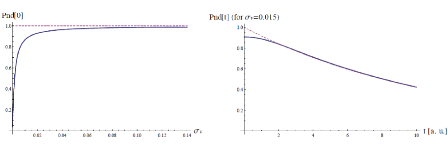
Figure 2: Left: $P_{nd}(0)$ as function of the velocity wave-packet spreading parameter $\sigma_{v}.$ Right: $P_{nd}(t)$ for the illustrative case $\sigma_{v}=0.015;$ after a transient non-exponential part, the standard formula (2) (dashed line) is a good approximation.

In Fig. 2, left panel, we plot $P_{nd}(0)$ as function of the spreading $\sigma_{v}$ for the particular choice $v_{0}=1/2$, $M=10$ [a. u.] and $\Gamma/M=1/100.$ The smaller is the spreading, the smaller is also the initial probability $P_{nd}(0)$. For $\sigma_{v}\rightarrow 0$ we reobtain a state with definite velocity and the overlap vanishes, as in Eq. (20). However, for increasing $\sigma_{v}$ one gets very quickly a state with $P_{nd}(0)\simeq 1,$ which could be rewritten –to a very good approximation– in the form given by Eq. (13). Thus, a state with definite velocity is an idealization which must be regarded with great care. In Fig. 2, right panel, we show also the behavior of $P_{nd}(t)$ (solid line) for the representative case $\sigma_{v}=0.015,$ in which $P_{nd}(0)=0.9.$ A part from a Zeno-like non exponential part at the beginning, it quickly reaches the expected behavior (dashed line) $e^{-\Gamma_{p}t}\simeq e^{-\tilde{\Gamma}_{p}t}=e^{-\Gamma t/\gamma_{0}}$ with $\gamma_{0}=(1-v_{0}^{2})^{-1/2}$, i.e. the standard formula is again a very good approximation, as expected. In the end of this section, we emphasize that the results depicted in Fig. 2 belong to the most important ones of the present manuscript.

6 Discussions and conclusions

The study of the decay law of fast moving unstable particles represents an interesting link between special relativity and QM and QFT. This is indeed an important subject which has received attention from valuable pioneering works [17, 18, 19, 20, 21, 22, 23, 24, 25] but which also needs further clarifications and investigations in order to be accepted by a larger part of the scientific community. Moreover, in view of the very recent revival of the subject (e.g. Refs. [25, 26, 30]), we think that new interesting results can be obtained in the near future in this interesting topic.

In the present work we have thus reviewed -especially in Sec. 2 and 4- some existing results, but we have also presented new (in some cases analytic) formulas on the subject. Moreover, in Sec. 3 and especially 5, we have presented our main novel results. We briefly reports the main points in the following paragraphs.

An unstable state with definite momentum $p$ has a decay width given by Eq. (8): it is slightly larger than the usual expression of Eq. (2). Thus, the lifetime is actually slightly smaller than what the time dilatation expression tells us. The standard “Einstein” formula remains however a very good approximation which can be used in all practical applications, see Fig. 1 for the numerical quantification of the deviation. It is an open question if the small deviation will be measured at some point in the future.

More realistically, an unstable state is a superposition of the form of Eq. (13). The non-decay probability is not given by the probability that the state is still the initial one, but one has to project onto the basis of unstable states with definite momentum. The outcome is given in Eq. (15) and can usually also be very well approximated by the Einstein formula. We also generalize the expressions to the completely arbitrary initial state of Eq. (17), whose associated non-decay probability is given by Eq. (18). The various cases described in this work can be obtained by taking proper limits of these general expressions.

A boost is a very subtle operation when applied to an unstable state of zero momentum/velocity. Namely, the boosted state is an eigenstate of velocity but has a zero overlap with the basis of undecayed states. Moreover, the probability that such a state remains unchanged over time shows a quite curious time-contraction feature, see Eq. (21), but this is not the non-decay probability. When allowing for a realistic spread in velocity, there is indeed a (usually large) overlap with the set of undecayed states, and the non-decay probability can be again be well described by the usual expression of Eq. (2), as expected, see Fig. 2.

In conclusion, as usual in QM and QFT, one should specify which observer (if Alice or Bob) is making the measurement. The reference frame of the detector is relevant.

In this work, we gave expressions for the non-decay probability in the most general form, but we did not discuss numerical examples in which deviations from the Breit-Wigner spectral function appear. We did so because we wanted first to focus on the exponential limit and because deviations are typically small. Moreover, the use of the exponential limit is also advantageous because the decay law is valid independently if and how many measurements are performed [8, 31]. However, it must be stressed that the study of non Breit-Wigner distributions is indeed very interesting, e.g. Ref. [25]. In this context, the study of numerical cases in which wave packets of the most general type and the implementation of realistic distributions is promising and constitutes an important outlook of the present work. Moreover, the investigations of decays of moving particles at late times might be of interest in cosmological particle physics because unstable particles can be very fast and may travel long distances for a long time.

Acknowledgments: I thank G. Pagliara, W. Florkowski, W. Broniowski, and J. Róg for useful discussions.

References

- [1] Schrödinger, Erwin (November 1935). Naturwissenschaften 23 (49): 807–812 (1935).
- [2] V. Weisskopf and E. P. Wigner, Z. Phys. 63 (1930) 54. V. Weisskopf and E. Wigner, Z. Phys. 65 (1930) 18. G. Breit, Handbuch der Physik 41, 1 (1959).
- [3] M. O. Scully and M. S. Zubairy (1997), Quantum optics, Cambridge UK: Cambridge University Press.
- [4] L. A. Khalfin, 1957 Zh. Eksp. Teor. Fiz. 33 1371. (Engl. trans. Sov. Phys. JETP 6 1053).
- [5] B. Misra and E. C. G. Sudarshan, J. Math. Phys. 18 (1977) 756
- [6] A. Degasperis, L. Fonda and G. C. Ghirardi, Nuovo Cim. A 21 (1973) 471.
- [7] L. Fonda, G. C. Ghirardi and A. Rimini, Rept. Prog. Phys. 41 (1978) 587.
- [8] K. Koshino and A. Shimizu, Phys. Rept. 412 (2005) 191.
- [9] P. Facchi, H. Nakazato, S. Pascazio Phys. Rev. Lett. 86 (2001) 2699-2703.
- [10] F. Giacosa, G. Pagliara, Mod. Phys. Lett. A26 (2011) 2247-2259. [arXiv:1005.4817 [hep-ph]]; F. Giacosa and G. Pagliara, Phys. Rev. D 88 (2013) 025010 [arXiv:1210.4192 [hep-ph]].
- [11] F. Giacosa, Found. Phys. 42 (2012) 1262 [arXiv:1110.5923 [nucl-th]].
- [12] S. R. Wilkinson, C. F. Bharucha, M. C. Fischer, K. W. Madison, P. R. Morrow, Q. Niu, B. Sundaram, M. G. Raizen, Nature 387, 575 (1997); M. C. Fischer, B. Gutiérrez-Medina and M. G. Raizen, Phys. Rev. Lett. 87, 040402 (2001).
- [13] C. Rothe, S. I. Hintschich, A. P. Monkman, Phys. Rev. Lett. 96 (2006)163601.
- [14] J. Bailey et al., Nature 268 (1977) 301. J. Bailey et al. [CERN-Mainz-Daresbury Collaboration], Nucl. Phys. B 150 (1979) 1.
- [15] T. D. Lee, Phys. Rev. 95 (1954) 1329-1334. C. B. Chiu, E. C. G. Sudarshan and G. Bhamathi, Phys. Rev. D 46 (1992) 3508.
- [16] P. R. Berman and G. W. Ford, Phys. Rev. A 82, Issue 2, 023818; A. G Kofman, G. Kurizki, and B. Sherman, Journal of Modern Optics, vol. 41, Issue 2, p.353-384 (1994); P. Facchi and S. Pascazio, Phys. Rev. A 62, 023804 (2000) [arXiv:quant-ph/9909043 ]; P. Facchi and S. Pascazio, Phys. Lett. A 241 (1998) 139 [arXiv:quant-ph/9905017]. F. Giacosa, Phys. Rev. A 88, 052131 (2013) [arXiv:1305.4467 [quant-ph]].
- [17] P. Exner, Phys. Rev. D 28 (1983) 2621.
- [18] L. A. Khalfin, Quantum Theory of unstable particles and relativity, PDMI Pewprint 6/1997.
- [19] M. I. Shirkokov, JINR E2 10614 (1977).
- [20] M. I. Shirokov, Int. J. Theor. Phys. 43 (2004) 1541.
- [21] M. I. Shirokov, arXiv:quant-ph/0508087
- [22] E.V. Stefanovich, Internation l Journal of Theoretical Physics, Volume 35, Issue 12, pp.2539-2554 (1996).
- [23] E. V. Stefanovich, arXiv:physics/0603043
- [24] E. V. Stefanovich, “Relativistic quantum dynamics: A Non-traditional perspective on space, time, particles, fields, and action-at-a-distance,” physics/0504062 [physics.gen-ph].
- [25] K. Urbanowski, Phys. Lett. B 737 (2014) 346 [arXiv:1408.6564 [hep-ph]].
- [26] S. A. Alavi and C. Giunti, Europhys. Lett. 109 (2015) 6, 60001 [arXiv:1412.3346 [quant-ph]].
- [27] K. A. Olive et al. (Particle Data Group), Chin. Phys. C38, 090001 (2014).
- [28] M. E. Peskin and D. V. Schroeder, “An Introduction to quantum field theory,” Reading, USA: Addison-Wesley (1995) 842 p.
- [29] K. Urbanowski, arXiv:1504.00794 [quant-ph].
- [30] K. Urbanowski, Adv. High Energy Phys. 2015 (2015) 461987.
- [31] F. Giacosa and G. Pagliara, Phys. Rev. A 90 (2014) 5, 052107 [arXiv:1405.6882 [quant-ph]].