Random and free observables saturate the Tsirelson bound for CHSH inequality

Abstract

Maximal violation of the CHSH-Bell inequality is usually said to be a feature of anticommuting observables. In this work we show that even random observables exhibit near-maximal violations of the CHSH-Bell inequality. To do this, we use the tools of free probability theory to analyze the commutators of large random matrices. Along the way, we introduce the notion of “free observables” which can be thought of as infinite-dimensional operators that reproduce the statistics of random matrices as their dimension tends towards infinity. We also study the fine-grained uncertainty of a sequence of free or random observables, and use this to construct a steering inequality with a large violation.

I Introduction

The notion of quantum mechanics violating local realism was first raised by the work of A. Einstein, B. Podolsky and N. Rosen EPR . This was put on a rigorous and general footing by the revolutionary 1964 paper of J. S. Bell Bell , which derived an inequality (now known as the Bell inequality) involving correlations of two observables. Bell showed that there is a constraint on any possible correlations obtained from local hidden variable models which can be violated by quantum measurements of entangled states. Later on, another Bell-type inequality which is more experimentally feasible was derived by J. F. Clauser, M. A. Horne, A. Shimony and R. A. Holt CHSH1969 . Since then, Bell inequalities have played a fundamental role in quantum theory and have had applications in quantum information science including cryptography, distributed computing, randomness generation and many others (see BCPSW2014 for a review).

In this paper, we mainly focus on the maximal violation of CHSH-Bell inequality CHSH1969 . It is well known that the Tsirelson bound $2\sqrt{2}$ for CHSH-Bell inequality was first obtained by Tsirelson Tsirelson1980 . And he also proved that the bound can be realized by using proper Pauli observables. Apart from the above qubit case, it is possible to find dichotomic observables in high dimension GP1992 ; BMR1992 , as well as in the continuous-variable (infinite dimension) case CPHZ2002 , to obtain the Tsirelson bound. Recently, Y. C. Liang et. al. LHBR2010 have studied the possibility of violation of CHSH-Bell inequality by random observables. For the bipartite qubits case, if two observers share a Bell state showed that random measure settings lead to a violation with probability $\approx 0.283$. However, for two qubits, the probability of the maximal violation is zero, and the probability of near-maximal violation is negligible.

Contrary to the case of qubits, our results show that the probability of near-maximal violation is large in high dimension. here near-maximal violations are approximately achieved with high probability by random high-dimensional observables. Previous methods of showing maximal violation were based on specific algebraic relations, namely, anti-commuting, and indeed there is a sense in which maximal violations imply anti-commutation on some subspace MYS2012 . However, this random approach reveals that there is another type of algebraic relations between observables which might lead to the Tsirelson bound of CHSH-Bell inequality. We call the observables, which satisfy those relations, free observables. This terminology is from a mathematical theory called free probability VDN1992 ; NS2006 . As we explain below, those free observables are freely independent in some quantum probability space, which is a quantum analogue of the classical probability space (see the section IV for the definition). A crucial point is that free observables can only exist in infinite dimension, and thus are experimentally infeasible. We also discuss finite-dimensional approximations (section IV.B) which are more experimentally plausible and for which the Tsirelson bound can be approximately obtained.

In another part of this work we study the fine-grained uncertainty relations of free or random observables, which was introduced by J. Oppenheim and S. Wehner OW2010 . It is more fundamental than the usual entropic uncertainty relations and it relates to the degree of violation of Bell inequalities (non-local games) OW2010 ; RGMH2015 . For a pair of free (random) observables, we can show that the degree of their uncertainty is 0. On the other hand, it is interesting that for a sequence of free (random) observables $A_{1},\ldots,A_{n}$ with $n>4,$ the fine-grained uncertainty is upper bounded by $\frac{1}{2}+\frac{1}{\sqrt{n}},$ which is the same as the one given by the anti-commuting observables. Therefore as a byproduct of above results, by using free (random) observables we can obtain one type of steering inequality with large violation that recently was studied in MRYHH2015 .

II Preliminaries

First, we introduce terminology. For a bipartite dichotomic Bell scenario, there are two space-like separated observers, say, Alice and Bob. Each of them is described by a $N$-dimensional Hilbert space $H_{N},$ and Alice (resp. Bob) chooses one of $n$ dichotomic (i.e. two-outcome) observables $A_{i}$ (resp. $B_{j}$) that will take results $\alpha_{i}$ (resp. $\beta_{j}$) from set $\{1,-1\}.$ Thus the observables are self-adjoint unitaries.

Next, recall the famous CHSH-Bell inequality CHSH1969 . If $\alpha_{1},\alpha_{2},\beta_{1},\beta_{2}$ are classically correlated random variables then

$$\left|\langle\alpha_{1}\beta_{1}\rangle+\langle\alpha_{1}\beta_{2}\rangle+\langle\alpha_{2}\beta_{1}\rangle-\langle\alpha_{2}\beta_{2}\rangle\right|\leq 2,$$ (1)

so we say that 2 is the largest classical value obtained by any local hidden variable model. In Tsirelson1980 , Tsirelson first proved that if the correlations are obtained by quantum theory then the quantum value of the CHSH-Bell inequality is $2\sqrt{2}$ (i.e., the Tsirelson bound). To see this, consider the following CHSH-Bell operator

$$B_{\text{CHSH}}=A_{1}\otimes B_{1}+A_{1}\otimes B_{2}+A_{2}\otimes B_{1}-A_{2}\otimes B_{2},$$ (2)

where $A_{i},B_{j},i,j=1,2$ are dichotomic observables. By choosing proper observables, e.g. $A_{1}=\sigma_{x},A_{2}=\sigma_{z},B_{1}=(\sigma_{x}+\sigma_{z})/\sqrt{2},B_{2}=(\sigma_{x}-\sigma_{z})/\sqrt{2},$ the norm (largest singular value) of the CHSH-Bell operator is $2\sqrt{2}.$ If $\mathcal{B}=B_{\text{CHSH}}^{2},$ then

$$\mathcal{B}=41\mkern-4.0mu{\rm l}-[A_{1},A_{2}]\otimes[B_{1},B_{2}].$$ (3)

If both parties choose compatible (commutative) observables, then $\mathcal{B}=41\mkern-4.0mu{\rm l}.$ Hence incompatible (non-commutative) observables are necessary for the violation of CHSH-Bell inequality BMR1992 . The Tsirelson bound is also determined by the eigenvalues of the commutators $[A_{1},A_{2}]$ and $[B_{1},B_{2}].$ More precisely, suppose the local dimension for each party is $N,$ and the eigenvalues of $[A_{1},A_{2}]$ (resp. $[B_{1},B_{2}]$) are $s_{1},\ldots,s_{N}$ (resp. $t_{1},\ldots,t_{N}$). Then we have BMR1992 :

$$\|\mathcal{B}\|=\max_{i,j}\{4-s_{i}t_{j}\}.$$ (4)

It is clear that if there exist eigenstates such that the eigenvalues of $[A_{1},A_{2}]$ (resp. $[B_{1},B_{2}]$) are $\pm 2,$ then $\|B_{\text{CHSH}}\|=2\sqrt{2}.$ In particular, anti-commuting dichotomic local observables, such as $\sigma_{x}$ and $\sigma_{z}$, will saturate the Tsirelson bound.

III A random approach to the Tsirelson bound

Suppose $D$ is a $N\times N$ deterministic diagonal matrix, where the diagonal terms of $D$ are either $1$ or $-1$ and $\operatorname{Tr}(D)=0$ where $Tr$ is the usual trace for matrices. It is easy to see that $D^{2}=1\mkern-4.0mu{\rm l}.$ Suppose unitaries $U_{i},i=1,\ldots,n$ are independent Haar-random matrices in the group of unitary matrices $U(N).$ Define the following random dichotomic observables:

$$A_{i}=U_{i}DU_{i}^{\dagger},\;i=1,\ldots,n.$$ (5)

We would like to establish results that hold with “high probability” over some natural distribution. Recall that we call a sequence of random variables $\{X_{N}\}_{N}$ convergent to $X$ almost surely in probability space $(\Omega,P),$ if $P\left(\lim_{N\to\infty}X_{N}=X\right)=1.$ With these notions, we claim that the Tsirelson bound of CHSH-Bell inequality can be obtained in high probability by using random dichotomic observables in sufficient large dimension. More precisely, we have following theorem:

Theorem 1

Let $A_{i}=U_{i}DU_{i}^{\dagger}$ and $B_{i}=V_{i}DV_{i}^{\dagger},i=1,2,$ where $U_{i},V_{i}$ are independent Haar-random unitaries in $U(N).$ Then we have

$$\lim_{N\to\infty}\|B_{\text{CHSH}}\|=2\sqrt{2},\;\;\text{almost surely}.$$ (6)

Above theorem could be understand as the following: with sufficient large dimension, the random dichotomic observables may saturate the Tsirelson bound of the CHSH-Bell inequality. We note here that in this approximate scenario, the shared state for Alice and Bob should not be fixed, otherwise it may not obtain any violation at all. To prove this theorem, we first need following lemma from NS2006 :

Lemma 1

[NS2006 ] Let $\mathcal{M}_{N}$ be the set of $N\times N$ matrices. Then for every $A\in\mathcal{M}_{N},$

$$\|A\|=\lim_{k\rightarrow\infty}\left(\operatorname{tr}_{N}\left((A^{\dagger}A)^{k}\right)\right)^{\frac{1}{2k}},$$ (7)

where $\operatorname{tr}_{N}=\operatorname{Tr}/N.$

Now denote $A=[A_{1},A_{2}]$ and $B=[B_{1},B_{2}].$ For any $k\in\mathbb{N}_{0},$ by we can use the binomial formula and equation (3) to obtain

$$\begin{split}\operatorname{tr}_{N^{2}}(\mathcal{B}^{k})&=\operatorname{tr}_{N^{2}}(41\mkern-4.0mu{\rm l}-A\otimes B)^{k}\\ &=\sum_{j=0}^{k}\binom{k}{j}4^{k-j}(-1)^{j}\operatorname{tr}_{N}(A^{j})\cdot\operatorname{tr}_{N}(B^{j}).\end{split}$$ (8)

Let us consider the term $\operatorname{tr}(A^{j}).$ Since $A_{1}A_{2}$ and $A_{2}A_{1}$ commute, again by binomial formula, we have

$$\operatorname{tr}_{N}(A^{j})=\sum_{l=0}^{j}\binom{j}{l}(-1)^{j-l}\operatorname{tr}_{N}((A_{1}A_{2})^{|2l-j|}).$$ (9)

Now we need the second key lemma (see Appendix B for the details of proof).

Lemma 2

Let $A_{i}=U_{i}DU_{i}^{\dagger},$ where $U_{i},i=1,\ldots,n\in U(N)$ are independent Haar random unitaries. Consider a sequence $i(1),\ldots,i(k)\in[n]$ satisfying $i(1)\neq i(2)\neq i(3)\neq\ldots i(k-1)\neq i(k).$ Then

$$\lim_{N\to\infty}\operatorname{tr}_{N}(A_{i(1)}A_{i(2)}\cdots A_{i(k)})=0,\;\;\text{almost surely}.$$ (10)

This lemma is mostly due to the work of B. Collins Collins2002 ; CS2004 , where he and other co-authors developed a method to calculate the moments of polynomial random variables on unitary groups. This method is called the Weingarten calculus and is in turn based on Weingarten1978 . As we will see in the next section, this lemma can be thought of as establishing the “asymptotic freeness” of these random matrices. Thus by Lemma 2, we have (almost surely)

$$\begin{split}\lim_{N\to\infty}\operatorname{tr}_{N}(A^{j})&=\sum_{l=0}^{j}\binom{j}{l}(-1)^{j-l}\lim_{N\to\infty}\operatorname{tr}_{N}((A_{1}A_{2})^{|2l-j|})\\ &=\left\{\begin{split}&(-1)^{j/2}\binom{j}{j/2},\;\;\text{j is even},\\ &0,\;\;\text{otherwise}.\end{split}\right.\end{split}$$ (11)

A similar estimate is also valid for the term $\operatorname{tr}_{N}(B^{j}).$ Therefore

$$\lim_{N\to\infty}\operatorname{tr}_{N^{2}}(\mathcal{B}^{k})=\sum_{j=0,\;\text{j is even}}^{k}\binom{k}{j}4^{k-j}\binom{j}{j/2}^{2}:=Q_{k},\;\;\text{almost surely}.$$ (12)

By Stirling’s formula, we have $\lim_{k\to\infty}(Q_{2k})^{1/2k}=8.$ In other words, for any $\epsilon>0,$ we can choose $k\in\mathbb{N},$ such that $(Q_{2k})^{1/2k}>8-\epsilon.$ Since $(\operatorname{tr}_{N^{2}}\mathcal{B}^{k})^{1/k}\leq\|\mathcal{B}\|$ for all $k\geq 1,$ then we have

$$\liminf_{N\to\infty}\|\mathcal{B}\|\geq(Q_{2k})^{1/2k}>8-\epsilon,\;\;\text{almost surely.}$$ (13)

On the other hand, due to Tsirelson’s inequality Tsirelson1980 we have $\|\mathcal{B}\|\leq 8$. Thus we complete our proof of Theorem 1.

IV A free approach to the Tsirelson bound

The random dichotomic observables do not satisfy the anti-commuting relations. In fact, random dichotomic observables are “asymptotically” freely independent, which was first established by Voiculescu V1991 in the case of the Gaussian unitary ensemble (GUE). That result builds a gorgeous bridge across two distinct mathematical branches–random matrix theory and free probability. In free probability theory, we will treat observables $A_{i},B_{j}$ as elements of a $C^{*}$-algebra $\mathcal{A},$ equipped with an unital (faithful) state $\phi$, where “state” means a linear map from $\mathcal{A}$ to $\mathbb{R}$, unital means $\phi(1\mkern-4.0mu{\rm l})=1$ and faithful means $\phi(AA^{*})=0\Rightarrow A=0.$ The pair $(\mathcal{A},\phi)$ is called a $C^{*}$-probability space, which is a quantum analogue of a classical probability space and we can call it a "quantum" probability space. For example, $(\mathcal{M}_{N},\operatorname{tr}_{N})$ is a $C^{*}$-probability space, where $\mathcal{M}_{N}$ is the set of $N\times N$ matrices. We refer to NS2006 for more details of quantum probability.

Lemma 2 inspires us to consider the following adaptation of definition of freeness to the case of dichotomic observables.

Definition 1

For given $C^{*}$-probability space $(\mathcal{A},\phi),$ dichotomic observables $A_{i},i\in I$ are called freely independent, if

$$\phi(A_{i(1)}A_{i(2)}\cdots A_{i(k)})=0$$ (14)

whenever we have following:

1. $k$ is positive; $i(1),i(2),\ldots,i(k)\in I$;

2. $\phi(A_{i(k)})=0$ for all $k$;

3. $i(1)\neq i(2),i(2)\neq i(3),\ldots,i(k-1)\neq i(k).$

For the special case $I=\{1,2\},$ the above conditions are equivalent to

$$\phi(A_{1})=\phi(A_{2})=\phi(A_{1}A_{2})=\phi(A_{2}A_{1})=\phi(A_{1}A_{2}A_{1})=\phi(A_{2}A_{1}A_{2})=\cdots=0.$$ (15)

However, finite-dimensional observables cannot be freely independent. In other words, for fixed $N,$ the $C^{*}$-probability space $(M_{N},\operatorname{tr}_{N})$ is too small to talk about freeness, and Definition 1 refers to an empty set. Fortunately if we consider the observables in infinite dimensional Hilbert space, it is possible for them to be freely independent in some $C^{*}$-probability space $(\mathcal{A},\phi).$ Furthermore, the derivations in Section III do not depend on the dimension. In order to use an infinite dimensional $C^{*}$-probability space $(\mathcal{A},\phi)$ instead of $(M_{N},\operatorname{tr}),$ we need only update Lemma 1 with an appropriate formula, which is achieved by (34) below. We conclude as follows.

Theorem 2

For the CHSH-Bell inequality, the Tsirelson bound can be obtained by using observables which are freely independent in their respective local system. More precisely, if $A_{1},A_{2}$ and $B_{1},B_{2}$ are freely independent in some $C^{*}$-probability space $(\mathcal{A},\phi),$ then we have $\|B_{\text{CHSH}}\|=2\sqrt{2}.$

This result is rather abstract, but in the next subsection, we will provide a concrete example which satisfies the conditions in this theorem.

IV.1 A concrete example in infinite dimension

For infinite-dimensional $C^{*}$-probability space, Definition 1 is meaningful. Now consider a group $G=\ast_{n}\mathbb{Z}_{2}$ and its associated Hilbert space $\ell_{2}(G).$ This notation refers to the $n$-fold free product of $\mathbb{Z}_{2}$ with itself; i.e. the infinite group $G$ with the the following elements: $g_{i_{1}},g_{i_{1}}g_{i_{2}},\ldots,g_{i_{1}}g_{i_{2}}\cdots g_{i_{n}},i_{1},\ldots,i_{n}=1,\ldots,n,$ where $g_{1},\ldots,g_{n}$ are the generators of the group $G$ whose only relations are $g_{i}^{2}=1$. The set $\{|g\rangle:g\in G\}$ forms an orthonormal basis of $\ell_{2}(G),$ thus the dimension of $\ell_{2}(G)$ is infinite. Let $\lambda:G\rightarrow B(\ell^{2}(G))$ be the left regular group representation, which is defined as:

$$\lambda(g)|h\rangle=|gh\rangle,\;\forall h\in G.$$ (16)

The reduced $C^{*}$-algebra $C^{*}_{\text{red}}(G)$ is defined as the norm closure of the linear span $\{\lambda(g),g\in G\},$ where the norm is the operator norm of $B(\ell_{2}(G)).$ There is a faithful trace state $\phi$ on $C^{*}_{\text{red}}(G)$ defined as

$$\phi\Big{(}\sum_{g}\alpha_{g}\lambda(g)\Big{)}:=\alpha_{e}.$$ (17)

Obviously $\phi(1\mkern-4.0mu{\rm l})=1.$ Hence $(C^{*}_{\text{red}}(G),\phi)$ is a $C^{*}$-probability space. If $g_{i}$ is the generator of the $i$-th copy of $\ast_{n}\mathbb{Z}_{2},i=1,2,\ldots,n$ then

$$A_{i}=\lambda(g_{i}),\;\;i=1,\ldots,n,$$ (18)

It is easy to check $A_{i},i=1,\ldots,n$ are self-adjoint unitaries and freely independent in $(C^{*}_{\text{red}}(G),\phi)$. We will choose the local Hilbert spaces of Alice and Bob to be $\ell_{2}(G),$ where $n=2.$ By using those free observables, we can obtain the quantum value $2\sqrt{2}$ for CHSH-Bell inequality. Note conjugating by a unitary preserves freeness of observables, i.e, if $A_{1},A_{2}$ are freely independent, then $UA_{1}U^{\dagger},UA_{2}U^{\dagger}$ are still freely independent for any unitary $U$. Since the norm of Bell operator does not change under the local unitary operation, we can simply assume $A_{1}=B_{1}=\lambda(g_{1}),A_{2}=B_{2}=\lambda(g_{2}).$

IV.2 Truncated free observables in finite dimension

In order to see how the freeness behaves in a simple and direct way, we will truncate the free observables given by last subsection to finite dimension. Denote the elements in $\ell_{2}(\ast_{2}\mathbb{Z}_{2})$ as follows:

$$\begin{array}[]{ccccccccc}\cdots&\left|g_{2}g_{1}g_{2}\right\rangle&\left|g_{2}g_{1}\right\rangle&\left|g_{2}\right\rangle&\left|e\right\rangle&\left|g_{1}\right\rangle&\left|g_{1}g_{2}\right\rangle&\left|g_{1}g_{2}g_{1}\right\rangle&\cdots\\ \updownarrow&\updownarrow&\updownarrow&\updownarrow&\updownarrow&\updownarrow&\updownarrow&\updownarrow&\updownarrow\\ \cdots&\left|-3\right\rangle&\left|-2\right\rangle&\left|-1\right\rangle&\left|0\right\rangle&\left|1\right\rangle&\left|2\right\rangle&\left|3\right\rangle&\cdots\end{array}.$$ (19)

With the above notation, we have

$$\left\{\begin{split}&\lambda(g_{1})|i\rangle=|j\rangle,\;i+j=1,\\ &\lambda(g_{2})|i\rangle=|j\rangle,\;i+j=-1.\end{split}\right.$$ (20)

where $i,j=\cdots,-1,0,1,\cdots$.

Now define $A_{1}^{(N)}$ and $A_{2}^{(N)}$ to be the truncation of the free observables to dimension $N=2l+1$ (i.e, we truncated the operators $\lambda(g_{1}),\lambda(g_{2})$ into the operators acting on $N$ dimension Hilbert space.). Then we have (see Figure 1):

$$A_{1}^{(N)}|i\rangle =|1-i\rangle, i=-l+1,\ldots,l$$ (21a)

$$A_{1}^{(N)}|-l\rangle =|-l\rangle,$$ (21b)

and

$$A_{2}^{(N)}|i\rangle =|-1-i\rangle, i=-l,\ldots,l-1$$ (22a)

$$A_{2}^{(N)}|l\rangle =|l\rangle.$$ (22b)

where $|i\rangle,i=-l,\ldots,l$ denotes the basis of the $N$ dimensional Hilbert space.

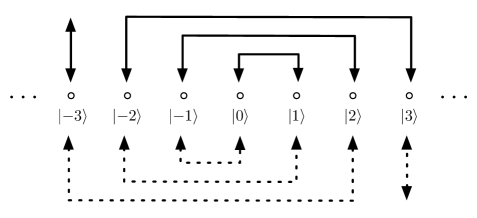
Figure 1: The solid line stands for $A_{1}^{(N)}$ and the dashed lines stands for $A_{2}^{(N)}$, where $N=7$. For example, the operator $A_{1}^{(N)}$ maps the vector $|0\rangle$ to $|1\rangle$ and vice versa. We only need to be careful for the vector $|-3\rangle$, where $A_{1}^{N}$ maps it to itself.

It is clear that $A_{1}^{(N)}$ and $A_{2}^{(N)}$ are self-adjoint unitaries. Thus they can be treated as a pair of dichotomic observables in an $N$-dimensional Hilbert space. Denote $S=A_{2}^{(N)}\circ A_{1}^{(N)},$ so that

$$S|j\rangle =|j-2\rangle, j=-l+2,\ldots,l$$ (23a)

$$S|-l+1\rangle =|l\rangle,$$ (23b)

$$S|-l\rangle =|l-1\rangle.$$ (23c)

By the following diagram it is easy to see that $S$ is a cycle in the permutation group $S_{N}.$

$$\begin{array}[]{ccccccccccc}|l\rangle&\longrightarrow&|l-2\rangle&\longrightarrow&|l-4\rangle&\longrightarrow&\cdots&\longrightarrow&|-l+2\rangle&\longrightarrow&|-l\rangle\\ \nwarrow&&&&&&&&&&\swarrow\\ &|-l+1\rangle&\longleftarrow&|-l+3\rangle&\longleftarrow&\cdots&\longleftarrow&|l-3\rangle&\longleftarrow&|l-1\rangle.&\end{array}$$ (24)

Now for the CHSH-Bell operator $B_{\text{CHSH}},$ by using those truncated free observables, we can show that the quantum value tends to $2\sqrt{2}$ as $N\rightarrow\infty.$ Then due to the fact that the eigenvalues of $S$ are $\lambda_{j}=\exp^{2\pi ij/N},j=0,\ldots,N-1,$ we have

$$\begin{split}\|B_{\text{CHSH}}^{2}\|&=\left\|41\mkern-4.0mu{\rm l}-[A_{1}^{(N)},A_{2}^{(N)}]\otimes[A_{1}^{(N)},A_{2}^{(N)}]\right\|\\ &=\left\|41\mkern-4.0mu{\rm l}-(S^{\dagger}-S)\otimes(S^{\dagger}-S)\right\|\\ &=\max_{j}\{4+4(\Im(\lambda_{j}))^{2}\}=\max_{j}\left\{4+4\sin^{2}{\frac{2\pi j}{N}}\right\}\\ &\thickapprox 4+4\left(1-O\left(\frac{1}{N^{2}}\right)\right)=8-O\left(\frac{1}{N^{2}}\right).\end{split}$$ (25)

Here for simplicity, we have assumed that Alice and Bob take same measurements. Therefore, we have following proposition:

Proposition 1

By using truncated free observables $A_{1}^{(N)},A_{2}^{(N)},N=2l+1,$ we can asymptotically obtain the Tsirelson bound for CHSH-Bell inequality, i.e, $\|B_{\text{CHSH}}\|=2\sqrt{2}-O(1/N^{2}).$

This result suggests the speed of the convergence mentioned in Theorem 1, namely, the Tsirelson bound will be saturated with the speed of $O(1/N)$ by using the random observables. However, the rigorous proof would need very careful and subtle analysis of Weingarten calculus.

V Fine-grained uncertainty relations for random (free) observables

The uncertainty principle and non-locality are two fundamental and intrinsic concepts of quantum theory which were quantitatively linked by J. Oppenheim and S. Wehner’s work OW2010 . There they introduced a notion called “fine-grained uncertainty relations” to quantify the “amount of uncertainty” in a particular physical theory. Suppose we have $n$ dichotomic observables $A_{i},i=1,\ldots,n,$ corresponding to measurement settings $P_{i}^{a}=\frac{1\mkern-4.0mu{\rm l}+(-1)^{a}A_{i}}{2},i=1,\ldots,n;a=0,1.$ The uncertainty of measurement settings $P_{i}^{0},i=1,\ldots,n$ is defined as:

$$\xi_{\vec{0}}=\sup_{\rho}\left\{\frac{1}{n}\sum_{i=1}^{n}\operatorname{Tr}(P_{i}^{0}\rho)\right\}=\frac{1}{2}+\frac{1}{2n}\sup_{\rho}\operatorname{Tr}\left(\sum_{i=1}^{n}A_{i}\rho\right).$$ (26)

Similarly, the uncertainty of $P_{i}^{1},i=1,\ldots,n$ is

$$\xi_{\vec{1}}=\sup_{\rho}\left\{\frac{1}{n}\sum_{i=1}^{n}\operatorname{Tr}(P_{i}^{1}\rho)\right\}=\frac{1}{2}-\frac{1}{2n}\sup_{\rho}\operatorname{Tr}\left(\sum_{i=1}^{n}A_{i}\rho\right).$$ (27)

Notice that

$$\sup_{\rho}\left|\operatorname{Tr}\left(\sum_{i=1}^{n}A_{i}\rho\right)\right|=\left\|\sum_{i=1}^{n}A_{i}\right\|.$$ (28)

Hence $\xi_{\vec{0}}=\xi_{\vec{1}}=\frac{1}{2}+\frac{1}{2n}\left\|\sum_{i=1}^{n}A_{i}\right\|.$ The state $\rho$ which can obtain $\xi_{\vec{x}}$ is called the maximally certain state for those measurement settings. If we assume $A_{i}$ are freely independent observables, then we have following proposition (see Appendix C and D for the proof):

Proposition 2

The fine-grained uncertainty for free observables $A_{i},i=1,\ldots,n,n>4$ is

$$\xi_{\vec{0}}=\xi_{\vec{1}}\leq\frac{1}{2}+\frac{1}{\sqrt{n}}<1.$$ (29)

The same results approximately hold for random observables $A_{i}=U_{i}DU_{i}^{\dagger},i=1,\ldots,n,n>4$ with high probability.

For the special case $n=2,$ we have $\|A_{1}+A_{2}\|=2.$ Thus for $n=2,$ $\xi_{\vec{0}}=\xi_{\vec{1}}=1$ (see Appendix D for random observables and Appendix E for free obervables). Interestingly, for truncated free observables we have

$$\begin{split}\|A_{1}^{(N)}+A_{2}^{(N)}\|^{2}&=21\mkern-4.0mu{\rm l}+S+S^{\dagger}=\max_{j}\{2+2\Re(\lambda_{j})\}\\ &=\max_{j}\left\{2+2\cos{\frac{2\pi j}{N}}\right\}=4.\end{split}$$ (30)

Thus for the truncated free observables, we always have $\xi_{\vec{0}}=\xi_{\vec{1}}=1$ regardless of what dimension we truncate to.

In a recent work, some of us show that there is a tight relationship between fine-grained uncertainty and violation of one specific steering inequality, called the linear steering inequality, which was first used in SJWP2010 to verify steering by experiment. It has following form:

$$S_{n}=\sum_{i=1}^{n}\langle\alpha_{i}A_{i}\rangle\leq C_{n},$$ (31)

where $C_{n}$ is called the local hidden state bound of $S_{n}.$ This bound can be calculated easily as follows SJWP2010 :

$$C_{n}=\sup_{\alpha_{i}=\pm 1}\left\|\sum_{i=1}^{n}\alpha_{i}A_{i}\right\|.$$ (32)

If the observables $A_{i}$ are chosen to be operators of a Clifford algebra, which are anti-commutative, a large (unbounded) violation can be obtained MRYHH2015 . Because the degree of the fine-grained uncertainty of free or random observables is the same order as that of anti-commuting observables, we find:

Corollary 1

If $A_{i},i=1,\ldots,n$ are chosen to be free observables, then the local hidden state bound of steering inequality $S_{n}=\sum_{i=1}^{n}\langle\alpha_{i}A_{i}\rangle\leq C_{n},$ is upper bounded by $2\sqrt{n}.$ The similar result holds for random observables with high probability.

Here we note that for the free case, we should also care about the quantum values of steering inequalities. Due to M. Navascués and D. Pérez-García’s work, there are two different ways to define them NG2012 . One is in a commuting way that means the system described by a total Hilbert space, and the other one is the total system described in a tensor form. As a matter of fact, they also used the free observables $\lambda(g_{i}),i=1,\ldots,n$ to define the linear steering inequality. They showed the quantum value defined in the commuting sense is $n,$ while in the tensor scenario is upper bounded by $2\sqrt{n-1}.$ So by their work, we can easily see that the local hidden state bound is upper bounded by $2\sqrt{n-1}$ for free observables. Their bound is even sharper than ours. However, we have provided another proof which is more focussed on the freeness property and is applicable to random observables.

VI Conclusions

In this paper, we show that random dichotomic observables generically achieve near-maximal violation of the CHSH-Bell inequality, approaching the Tsirelson bound in the limit of large dimension. This is despite the fact that these observables are not anti-commuting. Instead, due to Voiculescu’s theory, they are asymptotically freely independent. It means when the dimension increases, their behaviors tends to the ones of free observables in some quantum probability space. However, the quantum state that is optimal for the random observables is random as well, as it in general will depend on the observables. For a fixed state, random observables might not lead to any violation. Another main result of this paper is that we have considered the fine-grained uncertainty of a sequence of free or random observables. The degree of their uncertainty is as the same order as the one which is given by the anti-commuting observables. As a byproduct of this result, we can construct a linear steering inequality with large violation by using free or random observables. For further applications, free observables may be used for studying the quantum value of other type of Bell inequalities. Thus a natural question arises: Do free observables always maximally violate any Bell inequalities? Unfortunately, a quick answer is that we can consider the linear Bell operator $\sum_{i=1}^{n}A_{i}\otimes A_{i}.$ It is trivial since its quantum and classical value are both $n,$ while the quantum value given by free observables is upper bounded by $2\sqrt{n}$. However, it seems promising when considering other specific Bell inequalities. Since the free observables and their truncated ones are deterministic (constructive), another possible application is that this may be a new source of constructive examples of Bell inequality violations where previously only random ones were known.

Acknowledgments—We would like to thank Paweł Horodecki, Marek Bozejko, Mikael de la Salle, Yanqi Qiu and Junghee Ryu for valuable discussions. We also would like to thank the anonymous referee for her/his useful comments. This work is supported by ERC AdG QOLAPS, EU grant RAQUEL and the Foundation for Polish Science TEAM project cofinanced by the EU European Regional Development Fund. Z. Yin was partly supported by NSFC under Grant No.11301401. A. Rutkowski was supported by a postdoc internship decision number DEC– 2012/04/S/ST2/00002 and grant No. 2014/14/M/ST2/00818 from the Polish National Science Center. M. Marciniak was supported by EU project BRISQ2. Harrow was funded by NSF grants CCF-1111382 and CCF-1452616, ARO contract W911NF-12-1-0486 and a Leverhulme Trust Visiting Professorship VP2-2013-041.

Appendix

VI.1 $C^{*}$-probability space and freely independent

Definition 2

A $\ast$-probability space $(\mathcal{A},\phi)$ consists of an unital $\ast$-algebra $\mathcal{A}$ over $\mathbb{C}$ and an unital linear positive functional

$$\phi:\mathcal{A}\rightarrow\mathbb{C};\;\;\;\phi(1_{\mathcal{A}})=1.$$ (33)

The elements $a\in\mathcal{A}$ are called non-commutative random variables in $(\mathcal{A},\phi).$ A $C^{*}$-probability space is a $\ast$-probability space $(\mathcal{A},\phi)$ where $\mathcal{A}$ is an unital $C^{*}$-algebra.

If additionally we assume $\phi$ is faithful, we have for any $a\in\mathcal{A},$

$$\|a\|=\lim_{k\rightarrow\infty}\left(\phi\left((a^{*}a)^{k}\right)\right)^{\frac{1}{2k}}.$$ (34)

Definition 3

[12, 22] For given $C^{*}$-probability space $(\mathcal{A},\varphi),$ let $\mathcal{A}_{1},\ldots,\mathcal{A}_{n}$ be $\ast$-subalgebras of $\mathcal{A}$. They are said to be free if for all $a_{i}\in\mathcal{A}_{j(i)},i=1,\ldots n,\;j(i)\in\{1,\ldots,n\}$ such that $\phi(a_{i})=0$, one has

$$\phi(a_{1}a_{2}\cdots a_{n})=0$$ (35)

whenever $j(1)\neq j(2),j(2)\neq j(3),\ldots,j(n-1)\neq j(n).$ A sequence of random variables are said to be free if the unital subalgebras they generate are free.

VI.2 Proofs for Lemma 2

Lemma 2 is a direct corollary of the work of B. Collins [16]. A random variable $u\in(\mathcal{A},\phi)$ is called a Haar unitary when it is unitary and

$$\phi(u^{j})=\left\{\begin{split}&1,\;\;j=0,\\ &0,\;\;\text{otherwise}.\end{split}\right.$$ (36)

Since we have

$$\lim_{N\to\infty}\operatorname{tr}(D^{j})=\left\{\begin{split}&1,\;\;\text{j is even},\\ &0,\;\;\text{j is odd}.\end{split}\right.$$ (37)

Then there will exist a $C^{*}$-probability space $(\mathcal{A},\phi)$ and a random variable $d\in\mathcal{A},$ such that

$$\lim_{N\to\infty}\operatorname{tr}(D^{j})=\phi(d^{j}),\;\;\text{for all}\;j\geq 0.$$ (38)

Let $u_{1},\ldots,u_{n}$ be a sequence of Haar unitaries in $(\mathcal{A},\phi)$ which are freely independent together with $d$. We will give a concrete example of $u_{1},\ldots,u_{n},d$ in the end of this subsection. Let $E(\cdot)=\int\cdot\;d\mu,$ where $d\mu$ is the Haar measure on $U(N),$ then by the main theorem of [16, Theorem 3.1], we have following:

$$\begin{split}\lim_{N\to\infty}E\;\operatorname{tr}(A_{i(1)}A_{i(2)}\cdots A_{i(k)})&=\phi(u_{i(1)}du_{i(1)}^{*}\cdots u_{i(k)}du_{i(k)}^{*})\\ &=0,\end{split}$$ (39)

where the second equation comes from the freeness of $d,u_{1},\ldots,u_{n}.$ Moreover, by theorem of [16, Theorem 3.5]

$$P\left(\left|\operatorname{tr}(A_{i(1)}A_{i(2)}\cdots A_{i(k)})\right|\geq\epsilon\right)=O(N^{-2}).$$ (40)

Then by the Borel-Cantelli Lemma, for any $\epsilon>0,$

$$\limsup_{N\to\infty}\left|\operatorname{tr}(A_{i(1)}A_{i(2)}\cdots A_{i(k)})\right|\leq\epsilon,\;\;\text{almost surely}.$$ (41)

Hence

$$\lim_{N\to\infty}\operatorname{tr}(A_{i(1)}A_{i(2)}\cdots A_{i(k)})=0,\;\;\text{almost surely}.$$ (42)

A concrete example of $u_{1},\ldots,u_{n}$ and $d$.

Let $G=\ast_{2n+1}\mathbb{Z}_{2}$ and $g_{i},i=1,\ldots,2n+1$ be the generator of the $i$-th copy. Let $u_{i}=\lambda(g_{2i-1}g_{2i}),i=1,\ldots,n$ and $d=\lambda(g_{2n+1}).$ Then the $C^{*}$-probability we consider is $(C^{*}_{\text{red}}(G),\phi)$ which was defined in Subsection IV.1. It is easy to check that equations (36) and (38) hold. Thus $u_{i},i=1,\ldots,n$ are Haar unitaries in $(C^{*}_{\text{red}}(G),\phi).$ Moreover $u_{1},\ldots,u_{n},d$ are freely independent in $(C^{*}_{\text{red}}(G),\phi).$

VI.3 Proof of Proposition 2

Suppose the dichotomic observables $A_{i},i=1,\ldots,n$ are freely independent in some $C^{*}$-probability space $(\mathcal{A},\phi)$. Then by equation (34),

$$\begin{split}\left\|\sum_{i=1}^{n}A_{i}\right\|&=\lim_{k\rightarrow\infty}\left(\phi\left(\sum_{i=1}^{n}A_{i}\right)^{2k}\right)^{\frac{1}{2k}}\\ &=\lim_{k\rightarrow\infty}\left(\phi\left(\sum_{i(1),\ldots,i(2k)=1}^{n}A_{i(1)}\cdots A_{i(2k)}\right)\right)^{\frac{1}{2k}}.\end{split}$$ (43)

To estimate the above equation we need the following definitions and facts from combinatorics [12]. For a given set $\{1,\ldots,2k\},$ there is a partition $\pi=\{V_{1},\ldots,V_{s}\}$ of this set. $\pi$ is determined as follows: Two numbers $p$ and $q$ belong to the same block $V_{k}$ of $\pi$ if and only if $i(p)=i(q).$ There is a particular partition called pair partition, in which every block only contains two elements. A pair partition of $\{1,\ldots,2k\}$ is called non-crossing if there does not exist $1\leq p_{1}<q_{1}<p_{2}<q_{2}\leq 2k$ such that $p_{1}$ is paired with $p_{2}$ and $q_{1}$ is paired with $q_{2}.$ The number of non-crossing pair partitions of the set $\{1,\ldots,2k\}$ is given by the Catalan number $C_{k}=\frac{1}{k+1}\binom{2k}{k}$.

Now for the indices $i(1),\ldots,i(2k),$ if there exist a pair of adjacent indices which they belong to a same block, e.g. $i(s-1)=i(s),$ then we will shrink the indices $i(1),\ldots,i(2k)$ to $i(1),\ldots,i(s-2),\emptyset,i(s+1),\ldots,i(2k),$ since obviously $A_{i(s-1)}A_{i(s)}=1\mkern-4.0mu{\rm l}.$ According to this rule, we can shrink $\pi$ to a new partition $\tilde{\pi}$ on $\{1,\ldots,2t\},$ where $t\leq k.$ Hence we can divide $\pi$ into two groups:

Case 1. $\tilde{\pi}=\emptyset$.

Case $2.$ The indices in $\tilde{\pi}$ are satisfy condition (iii) in Definition 1, i.e, the adjacent indices are not equal.

We decompose $\phi\left(\sum_{i=1}^{n}A_{i}\right)^{2k}$ into two terms:

$$\phi\left(\sum_{i=1}^{n}A_{i}\right)^{2k}=\phi\sum_{\pi\in\Pi_{1}}\cdot+\phi\sum_{\pi\in\Pi_{2}}\cdot:=II_{1}+II_{2},$$ (44)

where the set of partitions $\Pi_{1}$ and $\Pi_{2}$ is defined as follows: Partition $\pi\in\Pi_{1}$ if and only if $\pi$ belongs to Case 1. And $\pi\in\Pi_{2}$ if and only if $\pi$ belongs to Case $2$.

By our assumption, i.e, freeness of $A_{i},$ $II_{2}=0.$ For the term $II_{1},$ it is easy to see that $II_{1}$ is equal to the cardinality of the set $\Pi_{1}.$ Due to shrink process, $\pi\in\Pi_{1}$ only if there is even number of elements for every block. Those partitions with even elements in every block can be realized in following process: First choosing an arbitrary non-crossing pair partition, then combining some proper blocks to one block. Hence the number of $\pi\in\Pi_{1}$ is upper bounded by $C_{k}n^{k}.$ Thus

$$\phi\left(\sum_{i=1}^{n}A_{i}\right)^{2k}\leq C_{k}n^{k}.$$ (45)

Therefore under our assumption,

$$\left\|\sum_{i=1}^{n}A_{i}\right\|=\lim_{k\rightarrow\infty}\left(\phi\left(\sum_{i=1}^{n}A_{i}\right)^{2k}\right)^{\frac{1}{2k}}\leq 2\sqrt{n}.$$ (46)

Note: For the local hidden state bound $C_{n}$ of steering inequality $S_{n}$ in equation (32), the variables $\alpha_{i}$ do not make any effort to the whole derivation. Thus $C_{n}$ is also upper bounded by $2\sqrt{n}.$

VI.4 Fine-grained uncertainty for random observables

In fact, the statement is a corollary of the work of B. Collins and C. Male [22]. Here we restate their result as following: Let $A_{i}=U_{i}DU_{i}^{\dagger},$ then there exist $C^{*}$-probability space $(\mathcal{A},\phi)$ and Haar unitaries $u_{1},\ldots,u_{n}$ which are freely independent of element $d\in\mathcal{A},$ such that

$$\lim_{N\to\infty}\left\|\sum_{i=1}^{n}A_{i}\right\|=\left\|\sum_{i=1}^{n}u_{i}du_{i}^{*}\right\|,\;\;\text{almost surely}.$$ (47)

Denote $a_{i}=u_{i}du_{i}^{*},$ it is easy to see that $a_{1},\ldots,a_{n}$ are freely independent in $(\mathcal{A},\phi).$ Hence due to a similar argument in Appendix C, we have $\left\|\sum_{i=1}^{n}u_{i}du_{i}^{*}\right\|\leq 2\sqrt{n}.$ Therefore we have following corollary:

Corollary 2

Let $A_{i}=U_{i}DU_{i}^{\dagger},i=1,\ldots,n,$ $U_{i}$ are independent random matrices in $U(N).$ Then we have

$$\lim_{N\to\infty}\left\|\sum_{i=1}^{n}A_{i}\right\|\leq 2\sqrt{n},\;\;\text{almost surely.}$$ (48)

For the special case $n=2,$ we have following corollary:

Corollary 3

Let $A_{i}=U_{i}DU_{i}^{\dagger},i=1,2,$ $U_{i}$ are independent random matrices in $U(N).$ Then we have

$$\lim_{N\to\infty}\left\|\sum_{i=1}^{2}A_{i}\right\|=2,\;\;\text{almost surely}.$$ (49)

Proof. For all $k\in\mathbb{N}_{0},$ then almost surely we have

$$\begin{split}\lim_{N\to\infty}\operatorname{tr}\left(A_{1}+A_{2}\right)^{2k}&=\sum_{j=0}^{k}\binom{k}{j}2^{k-j}\sum_{l=0}^{j}\binom{j}{l}\lim_{N\to\infty}\operatorname{tr}\left(A_{1}A_{2}\right)^{2l-j}\\ &=\sum_{j=0,\;\text{even}}^{k}\binom{k}{j}2^{k-j}\binom{j}{j/2}.\end{split}$$ (50)

Since $\lim_{k\to\infty}\left(\sum_{j=0,\;\text{even}}^{k}\binom{k}{j}2^{k-j}\binom{j}{j/2}\right)^{\frac{1}{2k}}=2,$ then by the standard argument in this sequel, we have

$$\liminf_{N\to\infty}\Big{\|}\sum_{i=1}^{2}A_{i}\Big{\|}\geq 2-\epsilon,\;\text{almost surely}.$$ (51)

On the other hand, $\Big{\|}\sum_{i=1}^{2}A_{i}\Big{\|}\leq 2$ is obvious.

VI.5 Maximally certain states for $\xi_{\vec{0}}$ and $\xi_{\vec{1}}$ in the case $n=2$

Let $A_{1}=\lambda(g_{1}),A_{2}=\lambda(g_{2}),$ where $g_{1},g_{2}$ are generator of group $\ast_{2}\mathbb{Z}_{2}.$ We need following notions.

Definition 4

A group G is amenable if there exists a state $\mu$ on $\ell_{\infty}(G)$ which is invariant under the left translation action: i.e. for all $s\in G$ and $f\in\ell_{\infty}(G),\mu(s\cdot f)=\mu(f).$

Definition 5

Let G be a group, a Følner net (sequence) is a net of non-empty finite subsets $F_{n}\subset G$ such that $|F_{n}\cap gF_{n}|/|F_{n}|\to 1$ for all $g\in G.$ Where $gF_{n}$ denotes the subset $\{gh:h\in F_{n}\}.$

For any $g\in G,$ there exists $N,$ such that for all $n\geq N,$ $g\in F_{n}.$ There are many characterizations of amenable groups.

Proposition 3

[23] Let G be a discrete group. The following are equivalent:

1. G is amenable;

2. G has a Følner net (sequence);

3. For any finite subset $E\subset G$, we have $\frac{1}{|E|}\left\|\sum_{g\in E}\lambda(g)\right\|=1.$

For instance, group $\ast_{2}\mathbb{Z}_{2}$ is amenable. Hence by above proposition, $\|\lambda(g_{1})+\lambda(g_{2})\|=2.$ With above notions, we can formally define a state

$$\rho_{n}=\frac{1}{|F_{n}|}\sum_{g,h\in F_{n}}|g\rangle\langle h|,$$ (52)

where $F_{n}$ is a Følner sequence of $G=\ast_{2}\mathbb{Z}_{2}.$ Now we have:

$$\begin{split}\lim_{n\rightarrow\infty}\operatorname{Tr}((\lambda(g_{1})+\lambda(g_{2}))\rho_{n})&=\lim_{n\to\infty}\frac{1}{|F_{n}|}\left(\sum_{g,h\in F_{n}}\langle h|g_{1}g\rangle+\sum_{g,h\in F_{n}}\langle h|g_{2}g\rangle\right)\\ &=\lim_{n\to\infty}\frac{1}{|F_{n}|}(|F_{n}\cap g_{1}F_{n}|+|F_{n}\cap g_{2}F_{n}|)=2,\end{split}$$ (53)

where for the second equation we have used the property of Følner sequence. Thus in this approximate sense, the fine-grained uncertainty of $A_{1}^{0}$ and $A_{2}^{0}$ is 1. Technically we can construct $\tilde{\rho}_{n}$ to approximate $\xi_{\vec{1}}.$ Firstly we define two subsets of $G=\ast_{2}{\mathbb{Z}_{2}}:$

$$G_{1}=\{g_{1},g_{1}g_{2},g_{1}g_{2}g_{1},\cdots\}\;\;\text{and}\;\;G_{2}=\{g_{2},g_{2}g_{1},g_{2}g_{1}g_{2},\cdots\}.$$ (54)

In fact, $G_{1}$ (resp. $G_{2}$) is the subset of wards which begin with $g_{1}$ (resp. $g_{2}$). It is easy to see $G_{1}\cup G_{2}\cup\{e\}=G.$ Now we define a state:

$$|\tilde{\phi}_{n}\rangle=\frac{1}{\sqrt{|F_{n}|}}\sum_{g\in F_{n}}e^{i\theta_{g}}|g\rangle,$$ (55)

where $F_{n}$ is still a Følner sequence of $G$ and

$$\theta_{g}=\left\{\begin{split}&\pi/2&\quad\quad g\in G_{1},\\ &-\pi/2&\quad\quad g\in G_{2},\\ &0&\quad\quad g=e.\end{split}\right.$$ (56)

Let $\tilde{\rho}_{n}=|\tilde{\phi}_{n}\rangle\langle\tilde{\phi}_{n}|,$ then we have

$$\begin{split}\lim_{n\to\infty}Tr((\lambda(g_{1})+\lambda(g_{2}))\tilde{\rho}_{n})&=\lim_{n\to\infty}\frac{1}{|F_{n}|}\sum_{g,h\in F_{n}}e^{i(\theta_{g}-\theta_{h})}\left(\langle h|g_{1}g\rangle+\langle h|g_{2}g\rangle\right)\\ &=\lim_{n\to\infty}\frac{1}{|F_{n}|}\left(\sum_{g\in F_{n}\cap g_{1}F_{n}}e^{i(\theta_{g}-\theta_{g_{1}g})}+\sum_{g\in F_{n}\cap g_{2}F_{n}}e^{i(\theta_{g}-\theta_{g_{2}g})}\right).\end{split}$$ (57)

For the first of term of right hand side, for large enough $n,$ we can say $e,g_{1}\in F_{n}.$ Therefore $e,g_{1}\in F_{n}\cap g_{1}F_{n}$ for large enough $n.$ Then we have

$$\begin{split}\frac{1}{|F_{n}|}\sum_{g\in F_{n}\cap g_{1}F_{n}}e^{i(\theta_{g}-\theta_{g_{1}g})}&=\frac{1}{|F_{n}|}\sum_{g\in F_{n}\cap g_{1}F_{n},g\neq\{e,g_{1}\}}e^{i(\theta_{g}-\theta_{g_{1}g})}+\frac{1}{|F_{n}|}e^{i(\theta_{e}-\theta_{g_{1}e})}+\frac{1}{|F_{n}|}e^{i(\theta_{g_{1}}-\theta_{g_{1}g_{1}})}\\ &=\frac{1}{|F_{n}|}\sum_{g\in F_{n}\cap g_{1}F_{n},g\neq\{e,g_{1}\}}e^{i\pi}=-\frac{|F_{n}\cap g_{1}F_{n}|-2}{|F_{n}|},\end{split}$$ (58)

where for the second equation we have used (56). A similar argument is valid for the second term of right hand side of (57). Thus finally we have

$$\lim_{n\to\infty}\operatorname{Tr}((\lambda(g_{1})+\lambda(g_{2}))\tilde{\rho}_{n})=-2.$$ (59)

VI.6 Quantum value of complex CHSH-Bell inequality

In this appendix we will consider a Bell inequality which has a similar form to the CHSH-Bell inequality. The Bell operator is defined as follows:

$$\mathcal{B}=A_{1}\otimes B_{1}+A_{1}\otimes B_{2}+A_{2}\otimes B_{1}+\omega A_{2}\otimes B_{2},$$ (60)

where $\omega=e^{\frac{2\pi i}{3}}.$ Here the observables are not dichotomic. Instead, there are three possible outcomes: $1,\omega,\omega^{2}.$ Thus $A_{i},B_{j}$ are required to be unitaries and satisfy $A_{i}^{3}=B_{j}^{3}=1\mkern-4.0mu{\rm l}$ for any $i,j=1,2.$ The classical value of this Bell functional is $\sqrt{7}.$

Now for the quantum value, we can assume $A_{1}=B_{1},A_{2}=B_{2}$ and $A_{1},A_{2}$ are freely independent in some $C^{*}$-probability space. Hence we have

$$\mathcal{B}\mathcal{B}^{\dagger}=31\mkern-4.0mu{\rm l}\otimes 1\mkern-4.0mu{\rm l}+(1\mkern-4.0mu{\rm l}-\omega A)\otimes(1\mkern-4.0mu{\rm l}-\omega A),$$ (61)

where $A=A_{1}A_{2}^{\dagger}+\omega A_{2}A_{1}^{\dagger}.$ By binomial formula we have

$$\operatorname{tr}(\mathcal{B}\mathcal{B}^{\dagger})^{k}=\sum_{j=0}^{k}\binom{k}{j}3^{k-j}\left(\sum_{l=0,\text{l is even}}^{j}\binom{j}{l}\binom{l}{l/2}\right)^{2}:=Q_{k}.$$ (62)

On one hand, by Stirling’s formula, for even $l,$ $\binom{l}{l/2}\leq 2^{l},$ thus

$$Q_{k}\leq\sum_{j=0}^{k}\binom{k}{j}3^{k-j}\left(\sum_{l=0}^{j}\binom{j}{l}2^{l}\right)^{2}=12^{k}.$$ (63)

By Lemma 1, we have $\|\mathcal{B}\|\leq 2\sqrt{3}.$ By a slightly adaption of the results in [24], where they provided a method to estimate the quantum value for given dichotomic Bell inequalities, we can conclude that $2\sqrt{3}$ is an upper bound for the quantum value of complex CHSH Bell inequality. In fact, this upper bound can be obtained by choosing:

$$A_{1}=B_{1}=\begin{pmatrix}&0&0&1\\ &\omega^{2}&0&0\\ &0&\omega&0\end{pmatrix},\;A_{2}=B_{2}=\begin{pmatrix}&0&0&-\omega\\ &0&1&0\\ &\omega^{2}&0&0\end{pmatrix}.$$ (64)

On the other hand,

$$\begin{split}Q_{2k}&=\sum_{j=0}^{k}\binom{2k}{2j}3^{2k-2j}\left(\sum_{l=0}^{j}\binom{2j}{2l}\binom{2l}{l}\right)^{2}+\sum_{j=1}^{k}\binom{2k}{2j-1}3^{2k-2j+1}\left(\sum_{l=0}^{j-1}\binom{2j-1}{2l}\binom{2l}{l}\right)^{2}\\ &\approx\sum_{j=0}^{k}\binom{2k}{2j}3^{2k-2j}\left(\sum_{l=0}^{j}\binom{2j}{2l}2^{2l}\right)^{2}+\sum_{j=1}^{k}\binom{2k}{2j-1}3^{2k-2j+1}\left(\sum_{l=0}^{j-1}\binom{2j-1}{2l}2^{2l}\right)^{2}\\ &\gtrsim\sum_{j=0}^{k}\binom{2k}{2j}3^{2k-2j}\left(\sum_{l=0}^{j}\binom{j}{l}2^{2l}\right)^{2}+\sum_{j=1}^{k}\binom{2k}{2j-1}3^{2k-2j+1}\left(\sum_{l=0}^{j-1}\binom{j-1}{l}2^{2l}\right)^{2}\\ &\approx\sum_{j=0}^{2k}\binom{2k}{j}3^{2k-j}5^{j}=8^{2k}.\end{split}$$ (65)

Therefore $\|\mathcal{B}\|\geq 2\sqrt{2}>\sqrt{7}.$

This method is also promising for the famous MABK Bell inequalities [25, 26].

References

- [1] A. Einstein, B. Podolsky and N. Rosen, Phys. Rev. 47, 777, (1935).
- [2] J. S. Bell, Physics, 1, 195 (1964).
- [3] J. F. Clauser, M. A. Horne, A. Shimony and R. A. Holt, Phys. Rev. Lett. 23, 880 (1969).
- [4] N. Brunner, D. Cavalcanti, S. Pironio, V. Scarani, S. Wehner, Rev. Mod. Phys. 86, 419 (2014).
- [5] B. S. Tsirelson, Lett. Math. Phys. 4, 93 (1980).
- [6] N. Gisin and A. Peres, Phys. Lett. A 162, 15-17 (1992).
- [7] S. L. Braunstein, A. Mann, and M. Revzen, Phys. Rev. Lett. 68, 3259 (1992).
- [8] Z. B. Chen, J. W. Pan, G. Hou, and Y. D. Zhang, Phys. Rev. Lett. 88, 040406 (2002).
- [9] Y. C. Liang, N. Harrigan, S. D. Bartlett, and T. Rudolph, Phys. Rev. Lett. 104, 050401 (2010).
- [10] M. McKague, T. H. Yang, V. Scarani. J. Phys. A: Math. Theor. 45 455304 (2012)
- [11] D. Voiculescu, K. J. Dykema, and A. Nica, Free Random Variables, CRM Monograph Series 1, AMS (1992).
- [12] A. Nica and R. Speicher, Lectures on the Combinatorics of Free Probability.
- [13] J. Oppenheim and S. Wehner, Science. 330, 1072 (2010).
- [14] R. Ramanathan, D. Goyeneche, P. Mironowicz, and P. Horodecki, Arxiv 1506.05100 (2015).
- [15] M. Marciniak, A. Rutkowski, Z. Yin, M. Horodecki, and R. Horodecki, Phys. Rev. Lett. 115, 170401 (2015).
- [16] B. Collins, Int. Math. Res. Not. 17, 953-982 (2002).
- [17] B. Collins and P. Śniady, Comm. Math. Phys. 264 (3), 773-795 (2004).
- [18] D. Weingarten, J. Math. Phys. 19, 999 (1978).
- [19] D. Voiculescu, Invent. Math. 104, 201-220 (1991).
- [20] D. J. Saunders, S. J. Jones, H. M. Wiseman and G. J. Pryde, Nature. Phys. 6, 845 (2010).
- [21] M. Navascués and D. Pérez-Garcí, Phys. Rev. Lett. 109, 160405 (2012).
- [22] B. Collins and C. Male, To appear in Annales Scientifique de l’ENS. ArXiv:1105.4345 (2013).
- [23] N. Brown and N. Ozawa, Graduate Studies in Mathematics, vol. 88, AMS (2008).
- [24] M. Epping, H. Kampermann, and D. Bruß, Phys. Rev. Lett. 111, 240404 (2013).
- [25] R. F. Werner and M. M. Wolf, Phys. Rev. A. 64, 032112 (2001).
- [26] M. Zukowski and C. Brukner, Phys. Rev. Lett. 88, 210401 (2002).