Magnetization reversal of an individual exchange biased permalloy nanotube
Abstract
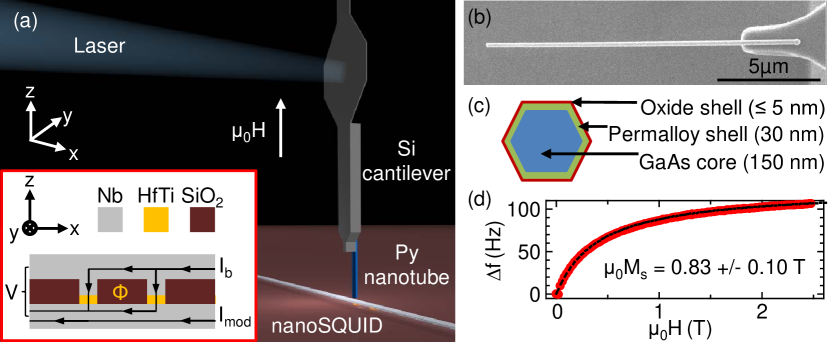
We investigate the magnetization reversal mechanism in an individual permalloy (Py) nanotube (NT) using a hybrid magnetometer consisting of a nanometer-scale SQUID (nanoSQUID) and a cantilever torque sensor. The Py NT is affixed to the tip of a Si cantilever and positioned in order to optimally couple its stray flux into a Nb nanoSQUID. We are thus able to measure both the NT’s volume magnetization by dynamic cantilever magnetometry and its stray flux using the nanoSQUID. We observe a training effect and temperature dependence in the magnetic hysteresis, suggesting an exchange bias. We find a low blocking temperature K, indicating the presence of a thin antiferromagnetic native oxide, as confirmed by X-ray absorption spectroscopy on similar samples. Furthermore, we measure changes in the shape of the magnetic hysteresis as a function of temperature and increased training. These observations show that the presence of a thin exchange-coupled native oxide modifies the magnetization reversal process at low temperatures. Complementary information obtained via cantilever and nanoSQUID magnetometry allows us to conclude that, in the absence of exchange coupling, this reversal process is nucleated at the NT’s ends and propagates along its length as predicted by theory.
Fabrication and characterization of magnetic nanostructures is motivated by a wide range of applications, including their use as media in dense magnetic memories (Parkin:2008, ), as magnetic sensors (Maqableh:2012, ), or as probes in high resolution magnetic imaging (Campanella:2011, ; Poggio:2010, ; Khizroev:2002, ). The desire for higher density memories, more sensitive sensors, and higher resolution imaging has pushed magnet size deep into the nanometer-scale. At these length scales, the stability of magnetization configurations strongly depends on geometry, defects, and minute levels of contamination. This sensitivity to imperfection makes the experimental realization of idealized systems such as ferromagnetic rods and tubes particularly challenging. Furthermore, due to the small total magnetic moment of each nanomagnet, conventional magnetometry techniques do not have the necessary sensitivity to measure individual nanostructures. As a result, measurements of their magnetic properties are often carried out on large ensembles, whose constituent nanomagnets have a distribution of size, shape, and orientation and – depending on the density – may interact with each other (Escrig:2008, ; EscrigAPL:2008, ). These complications conspire to make accurate characterization of the stable magnetization configurations and reversal processes difficult.
In order to obtain a clear understanding of the magnetic properties of ferromagnetic nanotubes (NTs), it is therefore advantageous to investigate individual specimens. Ferromagnetic NTs are particularly interesting nanomagnets because of their lack of a magnetic core. This geometry can make flux-closure magetization configurations more favorable than single-domain states (Escrig:2007, ). Flux-closure configurations are predicted to enable fast and reproducible magnetization reversal and they produce minimal stray magnetic fields, thereby reducing interactions between nearby nanomagnets. We therefore measure the magnetization and stray field hysteresis of an individual permalloy (Py) NT using a hybrid magnetometer. The magnetometer combines a sensitive mechanical sensor for dynamic cantilever magnetometry (DCM) and a nanometer-scale SQUID (nanoSQUID) for the measurement of stray magnetic fields. This measurement technique was first demonstrated on individual Ni NTs by Buchter et al.(Buchter:2013, ), who revealed the importance of morphological defects in altering the reversal process in real ferromagnetic NTs from the theoretical ideal.
Here, we study individual Py NTs. The fabrication process is based on evaporation instead of atomic layer deposition as used for Ni NTs (Ruffer:2012, ) and provides polycrystalline Py NTs with smooth surface that are morphologically closer to an idealized tube. Despite the geometrical perfection of the Py NTs, the measured low-temperature hysteresis curves reveal, that a thin exchange-coupled native oxide changes the reversal process (Meiklejohn:1956, ). Since the oxide is thin – likely less than 5 nm – these effects only appear at temperatures below 20 K. The role of the oxide is only apparent due to the sensitivity of the hybrid magnetometer to single NTs, since averaging effects would likely obscure the behavior in conventional measurements of NT ensembles. The strong effect of such a thin oxide layer on magnetic reversal, points to the importance of gaining further control of the fabrication of ferromagnetic NTs. At the same time, the results indicate that engineered oxide layers could be used to pin or otherwise control the magnetic configurations of magnetic NTs.
In order to fabricate the Py NTs, GaAs nanowires grown by molecular beam epitaxy are used as templates. These nanowires are 10 to 20 m long and have hexagonal cross-sections with a width nm at their widest point. Tubes of magnetic material are formed by thermally evaporating a nm polycristalline Py shell onto the template nanowires. For this deposition, the low density GaAs nanowire wafer is mounted under 35∘ angle and continuously rotated in order to achieve a conformal coating. The films fabricated in this process are very smooth, show no discontinuities and the roughness is less then nm. Individual Py NTs are then selected and transferred from the wafer to the end of a Si cantilever using high precision hydraulic micro-manipulators (Narishige MMO-202ND) mounted under an optical microscope. Each NT is attached parallel to the cantilever’s long axis, such that it protrudes from its end by m. The NT studied in this work is m long, and has a magnetic volume m3.
In our hybrid magnetometer, the single-crystal Si cantilever serves two purposes: 1) as the torque transducer in DCM measurements of the NT and 2) as a platform for positioning the NT such that stray magnetic fields from its tip couple to the nanoSQUID. It is m long, m wide and m thick and has a m thick and m long mass at its end to suppress higher order modes (Chui:2003, ). The NT-tipped cantilever hangs in the pendulum geometry above the nanoSQUID in a vacuum chamber at the bottom of a temperature variable He3 cryostat. This system is capable of temperatures down to K and magnetic fields up to T along the long axis of the cantilever (). The read-out of the cantilever deflection is achieved through a laser interferometer. We use a temperature controlled nm fiber-coupled DFB laser diode and an interferometer cavity formed between the cleaved end of an optical fibre and the m wide paddle of the Si cantilever (Rugar:1989, ). By feeding the measured displacement signal through a field-programmable gate array (National Instruments) and back to a piezo-electric actuator mechanically coupled to the cantilever, we self-oscillate the cantilever at its mechanical resonance frequency . The oscillation amplitude is stabilized to nm, for which the deflection angle , allowing for fast and accurate determination of . At a temperature of K and far from any surface the cantilever has an intrinsic resonance frequency of Hz and a quality factor . The spring constant N/m is determined by thermal noise measurements at different temperatures.
In order to control the relative position of the NT and the nanoSQUID, the nanoSQUID is mounted on a three dimensional piezoelectric positioning stage (Attocube). We use a direct current nanoSQUID containing two superconductor-normal metal-superconductor Josephson junctions (JJs) in a microstrip geometry (WoelbingAPL:2013, ). Two nm wide and nm thick Nb strips lie on top of each other and are separated by a nm thick SiO2 insulating layer. To form the m2 SQUID loop, the Nb strips are connected by two Nb/HfTi/Nb JJs with nm2 area and a nm thick HfTi barrier. Using a cryogenic series SQUID array as a low noise amplifier in a magnetically and electrically shielded environment and Magnicon XXF-1 read-out electronics, the described nanoSQUID shows a white rms flux noise n/Hz1/2 between 1 and 10 kHz. Here, is the magnetic flux quantum. At lower frequencies, the noise has a 1/f-like spectrum with a corner frequency around 200 Hz (see supplementary material).
We first investigate the NT sample through high-field DCM as plotted in Fig. 1d). The field is swept from T to T in mT increments, while the frequency shift of the cantilever is measured. The NT is composed of a Py shell that is known to be magnetically isotropic at room temperature. At small , the polycrystalline morphology is expected to average out any magnetocrystalline anisotropy. Given the latter and given the large aspect ratio of the NT, its anisotropy energy is dominated by shape effect. Therefore, the data are fit to an analytical model describing a Stoner-Wohlfarth particle with shape anisotropy (Weber:2012, ). In this model, the NT is idealized as a uniformly magnetized magnet whose magnetization rotates in unison. For applied along the easy axis of a sample with large shape anisotropy – as in this case – the magnetization is forced to be either parallel or anti-parallel to the applied field. As a result, this model is an excellent approximation for most of the field range, except in the regions of magnetic reversal. The model predicts a DCM frequency shift given by,
| (1) |
where is the permeability of free space, is the volume of the Py NT, is the effective length of the cantilever for its fundamental mode, is the saturation magnetization, and is the effective uniaxial demagnetization factor along (Weber:2012, ; Gross:2015, ). The two solutions are valid for and respectively, which for the NT’s easy-axis anisotropy () results in a region of bistability, allowing for magnetic hysteresis. By fitting the measurements shown in Fig.1d) with this expression, we extract T and as fit parameters. Input parameters are , , , and , which are all set to their measured values. The saturation magnetization measured for the Py NT is smaller than the literature value T (Thiaville:2005, ) for bulk Py. This discrepancy may be the result of an overestimation of the NT volume due to the oxide layer present on the surface or due to other imperfections in the growth of the film. The measured demagnetization factor, however, is in excellent agreement with what can be calculated by approximating the NT as a hollow cylinder, ignoring its hexagonal cross-section. The main contribution to the error in the extracted values stems from the NT volume, which is difficult to determine precisely. We calculate using the NT dimensions extracted from scanning electron micrographs (SEMs) of the Py shell thickness. A further source of error is the determination of the cantilever’s spring constant.
We now turn to the low-field behavior of the sample and the investigation of exchange bias. As key feature of exchange bias systems, we start by exploring the training effect of our sample. For initialization, the sample chamber is heated above K. The subsequent cool-down to K is done with an applied magnetic field of mT, in order to create a defined state of magnetization in the NT. Exploiting the duality of our hybrid magnetometer, we measure both the stray magnetic flux generated by the NT with the nanoSQUID and the integrated magnetization by DCM. For the nanoSQUID measurements, the NT-tipped cantilever is positioned for optimal coupling at height m above the nanoSQUID’s top electrode (NagelPRB:2013, ; Buchter:2013, ). Despite this proximity of the nanoSQUID to the NT, the magnetic fields produced by the bias and modulation currents running through the nanoSQUID and its superconducting leads are much less than mT at the position of the NT tip and do not significantly influence its magnetization state. Measurements of DCM, on the other hand, are carried out with the NT several tens of m away from the nanoSQUID in . This large spacing avoids spurious magnetic torque generated by the magnetic field gradients of the nanoSQUID, which otherwise complicate conversion of measured by DCM into magnetization .
In both cases, the magnetic field is swept first from mT to mT and subsequently between mT until ten full hysteresis loops are completed.
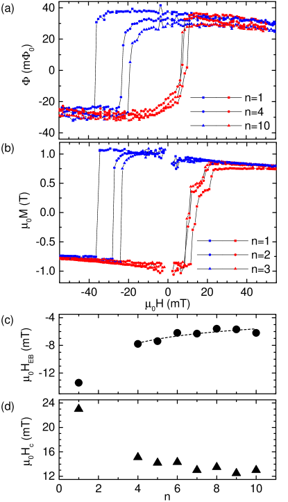
Fig. 2a) shows several iterations of magnetic hysteresis of the stray flux emanating from the NT measured by the nanoSQUID. In order to isolate the magnetic flux emerging from the Py NT from the spurious flux due to the external field threading through the slightly misaligned nanoSQUID, we record a reference sweep with the NT retracted tens of m from the substrate. These reference data, which exclude effects due to the NT, are then used both to subtract spurious flux and as a calibration of the magnetic field-axis (Buchter:2013, ). The blue squares show the first sweep from mT to mT. The flux from the NT starts at m and slightly increases to m at mT. This measurement artefact is the result of a slight temperature difference between the loop and the reference sweep. Thermal drift developing in the timespan of approximately hours between the two measurements alters the nanoSQUID’s response. Magnetization reversal takes place in a field range from mT to mT with a coercive field of mT. The reversal sets in by a steady decrease in flux of m followed by a large, abrupt change of m. Following the subsequent up-sweep (red squares), the temperature-induced slope can again be identified. In this case, reversal takes place over a wider field range than in the down-sweep, from mT to mT with a coercive field mT. We first observe a steady decrease of m of flux followed by a region of steeper change in flux (in the range of m), and ending with a final discontinuity of m. The total width of the loop is identified as the coercivity mT. We attribute the strong asymmetry of the hysteresis along the field axis to the exchange bias effect as will be detailed below. The corresponding parameter, the exchange-bias field, is defined as mT.
Subsequent sweeps show similar behavior, although with a progressive decrease in , as seen in the representative sweeps of Fig. 2a). Following the blue triangles of the sweep, we observe a smaller thermal drift effect than in the -loop due to the proximity in time between the -loop and the reference sweep taken at the end of the series. On the down-sweep, from mT to mT, the flux coupled into the nanoSQUID steadily decreases by m, followed by two abrupt switching events until the reversal process completes at mT. The reversal process on the up-sweep starts at mT with a continuous reduction of stray field of m over a range of mT. This continuous reversal is then followed by abrupt switching events until the process completes at mT. The most striking deviations from the first loop are the reduced width of the hysteresis loop – now mT – and the reduction of the exchange bias field mT. These findings are summarized in Fig. 2c), where and for to are plotted. decreases by mT until , after which point it stabilizes at mT. reduces by mT within the first seven loops until a saturation at mT. Past studies showed that the evolution of can be described by the following formula especially in the case of a polycrystalline antiferromagnet (NoguesEB:1999, ; Binek:2004, ; Paccard:1966, ):
| (2) |
where is a system dependent parameter and and are the exchange bias fields after loops and in the limit of infinite number of loops respectively. The fit for is shown as dashed line in Fig. 2c). The data are reasonably described by this power-law with deviations likely due to the inhomogeneity (in composition and thickness) of the naturally oxidized antiferromagnetic layer. As fit parameters we obtain mT and mT, whose magnitudes are of the same order as seen in literature (ProencaPRB:2013, ). Note also that as a function of training (increasing ), the hysteresis loop becomes more symmetric, losing the difference in the shape of the magnetization reversal for up- and down-sweeps. In particular, the abrupt reversal seen on the initial down-sweep is in stark contrast with the rounded transitions of later sweeps.
After an identical initialization and field-cooling procedure, DCM data are taken further away from the nanoSQUID, under otherwise identical measurement conditions. The magnetization hysteresis, shown in Fig. 2b), can be extracted from measurements of at low applied magnetic fields, by taking the limit of (1) for and solving for : (Gross:2015, ). Such data reflect the integrated magnetization of the entire NT, rather than the magnetization of the NT end closest to the substrate, as do the nanoSQUID measurements. The behavior of and reproduces what we observe with the nanoSQUID. Nevertheless, differences are observable in the appearance of the magnetization reversals. For the down-sweep, the single step magnetization reversal measured by DCM resembles that measured by the nanoSQUID. The reversal on the up-sweep shows a two-stage behavior, including an intermediate plateau, different than the continuous reversal followed by an abrupt switching seen in the corresponding nanoSQUID data. For , the down-sweep reversal gradually develops an initial stage of coherent reversal before discontinuous switching. Most strikingly, the coherent reversal seen in the nanoSQUID measurements, precedes the beginnings of any reversal observed by DCM. The discontinuous steps seen in the nanoSQUID sweeps coincide with the first discontinuous steps observed in DCM. The plateau and second discontinous reversal measured in DCM corresponds to a portion of the nanoSQUID hysteresis that has already reached saturation.
These findings lead us to two conclusions. First, the differences observed in the hysteresis measured by the nanoSQUID and by DCM indicate that magnetization reversal likely nucleates at the ends of the NT and subsequently propagates throughout its length, as predicted by theory (Landeros:2009, ). In this picture, vortex configurations form at the NT ends, begin tilting in the direction of the applied field, and subsequently cause magnetization reversal by propagating throughout the length of the tube and discontinuously switching to a uniform configuration aligned along the applied field. This kind of reversal is consistent with nanoSQUID measurements that show a smooth reversible reduction in stray field, which precede any deviation of from saturation registered by DCM. The subsequent irreversible change in the hysteresis is then registered both in the nanoSQUID and DCM measurements, thus apparently occuring throughout the NT and not only at the ends. The final stages of reversal seen in DCM, i.e. the plateau and second discontinuous step, appear to occur far from the NT end, since at this stage the nanoSQUID already shows a saturated signal. In short, the measurements appear consistent with the theoretical picture of reversal nucleation at the NT ends, considering that the nanoSQUID is sensitive to magnetization located at the NT end and DCM is sensitive to the total magnetization integrated throughout the NT. Unlike the Ni NTs measured by Buchter et al. (Buchter:2013, ), whose reversal did not nucleate at the ends most likely due to imperfections in their structure, these Py NTs appear to behave like the idealized magnetic NTs considered in theoretical calculations.
Second, the exchange bias effect influences the nature of the reversal process of the NT, as manifested in the changing shape of the hysteresis as a function of training. In particular, for small , the down-sweep magnetization reversal occurs almost exclusively through a single irreversible change, while the up-sweep reversal and both reversals for large contain both reversible rotation of magnetization and irreversible switching. The antiferromagnetic layer, in its initial configuration, appears therefore to pin the magnetization of the NT on the down-sweep, favoring reversal by abrupt domain nucleation and propagation. The exchange-coupled layer may thus suppress nucleation and initial coherent reversal through vortex cofigurations at the NT’s ends.
We next investigate the temperature dependence of the exchange bias effect in the Py NT. Hysteresis loops are measured by DCM in a temperature range between K and K. Concurrent measurements with the nanoSQUID are not possible since the device’s performance is strongly temperature dependent and above the critical temperature of Nb ( K), operation of the nanoSQUID is impossible. In order to ensure that our measurements are not obscured by training effects, we measure the temperature dependence after the extensive training of the NT, such that and are constant with increasing . In Fig. 3a), we plot three representative data sets at K for convenient comparison.
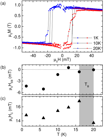
For each temperature, a hysteresis loop is measured for a field interval of mT. Following the blue squares between and mT, the magnetization remains constant around T at K. At mT the magnetization reversal process sets in by a continuous decrease of magnetization by T followed by an abrupt irreversible reversal step. Then over a range of mT a plateau forms which is followed by a smaller discontinuity in magnetization to complete the magnetization reversal. This second stage of reversal vanishes at higher temperatures, resulting in a reversal which occurs almost exclusively through a single irreversible change for both down- and up-sweeps. Proenca et al. observe a similar two-stage reversal in an ensemble of Co NTs (ProencaPRB:2013, ), with the second harder process also vanishing at high temperature. They thus connect this second stage of reversal to the exchange bias coupling. In contrast to our observations on a single Py NT, the coherent rotation measured in the Co/CoO arrays was extended over a much wider field range. Averaging over a distribution of different NTs in the array provides a possible explanation for this difference. In particular, NTs in the array appear in a distribution of shapes and sizes. In addition, NTs in both studies are oxidized naturally in an uncontrolled manner, allowing for a distribution of oxide thicknesses within an array. Since exchange bias crucially depends on film characteristics, including graininess and thickness, the hysteresis loops of the NT arrays are likely broadened by the distribution of different NTs in the array. For a detailed understanding, measurements of single NTs are therefore critical.
At K (triangles) the hysteresis loop measured in the Py NT shows perfectly symmetric behavior. This symmetry, combined with the observed reduction of and vanishing , indicates that the NT has reached the Py/oxide system’s blocking temperature . and are plotted over the whole temperature range in Fig. 3b) allowing for the determination of K. After decreases with rising temperature we find mT above K, indicating a blocking temperature in this regime. A more precise determination is possible, taking into account. With increasing temperature the coercivity shows a steady increase from mT to mT until K. At K, the next investigated temperature, drops below mT. This overall behavior is in line with previous studies (Kosub:2012, ) and allows us to determine a blocking temperature K.
This very low blocking temperature deviates drastically from the bulk values of the Néel temperatures of the possible native oxides of Py, which are all well above K. This deviation suggests that the oxide layer is very thin – in the range of to nm – and has a grainy and non-homogeneous structure (Cortie:2012, ; NoguesNano:2005, ; NoguesEB:1999, ). Indeed, similar blocking temperatures around K have been previously found for naturally oxidized Py thin films (Fulcomer:1972, ). The decreasing extent of the continuous reversal region with increasing temperature could be the result of the inhomogeneity and graininess of the oxide shell. Assuming grains of different dimensions, the anti-ferromagnetic order could be gradually lost in different sections of the shell with increasing temperature, thus leading to a gradual temperature-dependent change in the reversal behavior. Note that the temperature dependence of the reversal process provides further evidence that the exchange bias has a direct influence on the nature of the magnetization reversal in the Py NT.
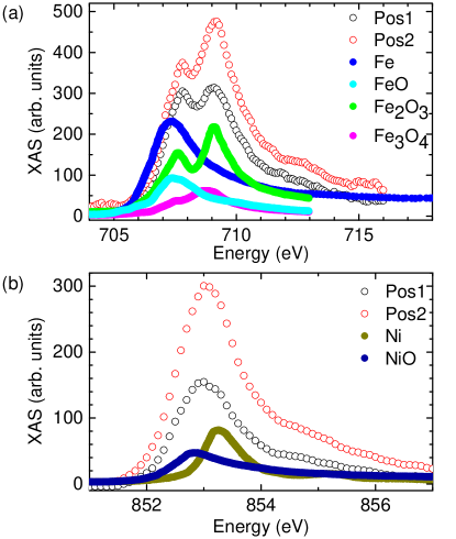
Given the measured exchange coupling, we investigate the nature of the native oxide present on the Py NTs using spatially resolved X-ray absorption spectroscopy (XAS) by means of X-ray photo-emission electron microscopy (PEEM). The experiments are performed using the PEEM instrument at the surface/interface:microscopy beamline of the Swiss Light Source at Paul Scherrer Institute (LeGuyader:2012, ). NTs from the same growth wafer as the one used in the magnetometry experiment are investigated. For the PEEM study the NTs are transferred to a Si substrate with the aid of the aforementioned micromanipulators and transferred into the microscope. X-ray PEEM provides a spatial map of the local X-ray absorption cross section. By recording such maps as a function of the photon energy it is possible to record local X-ray absorption spectra. Details are described, e.g., in Refs. (FraileRodriguez:2007, ; Vaz:2014, ). The spatial resolution of the instrument is between and nm and thus enables us to perform XAS at various positions along the NT. We focus on XAS in the vicinity of the L3 edges of Fe and Ni to study possible oxidation of the Py at different positions along the NT. Two measurement positions along a NT are chosen (at Pos 1: the NT’s broken end and another at Pos 2: close to the tip ). One additional section on the substrate is chosen to allow for background subtraction. The spectra are recorded using circularly polarized X-rays. polarized light is used first, then after correcting for mechanical drift, the polarization is changed to (FraileRodriguez:2010, ). This procedure is repeated successively for each position on the NT. Isotropic spectra are obtained by averaging data according to .
Two representative spectra measured at the L3 edge of Fe at Pos 1 and at Pos 2 are plotted in Fig. 4a). The data resemble typical spectra of oxidized Fe and thus suggest the presence of a Py oxide layer on the Py NT. They reveal Fe in different oxidation states in the Py oxide shell in addition to metallic Fe in the Py core, similar to what is observed in oxidized Fe surfaces, cf. Ref. (Vaz:2014, ). For comparison, reference data of pure Fe, FeO, Fe2O3 and Fe3O4 taken from Regan et al. (Regan:2001, ) are also plotted in Fig. 4a). The oxidation state of the present NT as seen at the Fe L3 edge is compatible with previous reports on comparable Py systems, which identify FeO or -Fe2O3 in the native oxide of Py (Salou:2008, ; Fitzsimmons:2006, ). However, comparing the spectra measured at Pos 1 and 2 further shows that the oxide layer is not homogeneous in composition as indicated by the different ratio of the peaks at and eV and by the varying signal amplitude, which we assign to the differences in mechanical treatment when picking up the NT. In order to resolve the presence of NiO, we also measure spectra at the Ni L3 edge between and eV. In Fig.4b) two representative curves are plotted for Pos 1 and 2 along with reference data for Ni and NiO from Regan et al. (Regan:2001, ). The Py NT’s data are compatible with a superposition of spectra of NiO and metallic Ni, which suggests the presence of a layer of NiO, in agreement with previous studies (Salou:2008, ; Fitzsimmons:2006, ).
These results point to a layered composition of oxidized Py in the following sequence: Py/(-Fe2O3 or FeO)/NiO (Fitzsimmons:2006, ). All three oxides are antiferromagnetically ordered below a certain ordering temperature (FeO: K, -Fe2O3: K, NiO: K) in the bulk (Duo:2010, ). The overall thickness of the oxide layer is estimated to be in the range of nm. This estimate is based on previous studies in literature (Salou:2008, ; Fitzsimmons:2006, ) and consistent with the fact that we detect a XAS signature from the metallic Py in our sample with the typical probing depth of X-PEEM being about nm. In such thin layers magnetic order temperatures are usually strongly reduced when compared to the bulk and thus might explain why exchange bias in the present Py NTs is only observed at temperatures below K.
In conclusion, in the absence of an exchange bias coupling with an unintentional antiferromagnetic oxide shell, we find strong evidence that the Py NT reverses its magnetization through the nucleation of a vortex configuration at its end followed by an irreversible switching process, as predicted by theory. However, below K and before field training, we observe that the few-nanometer-thick native oxide on the NT alters the process of magnetization reversal. In particular, the non-equilibrium antiferromagnetic configuration of the oxide appears to pin the magnetization of the NT and suppresses the nucleation of the magnetic vortices at the NT ends for one of the sweep directions. Therefore, in order to control magnetization reversal in Py NTs, one must control either the nature of the oxide capping layer or work well above the determined blocking temperature K, where exchange bias is not effective. These insights come as a direct result of our hybrid magnetometer’s ability to measure both the behavior of the magnetic moments at the end of the NT and the magnetization integrated throughout its volume. Applying this technique for the investigation of reversal processes in other types of nanomagnets appears to be a promising path for future experiments.
Acknowledgements.
The authors thank Alan Farhan for technical assistance and acknowledge support from the Canton Aargau, the SNI, the SNF under Grant No. 200020-159893, the DFG via Projects No. GR 1640/5-2 in SPP 1538 SpinCaT, KO 1303/13-1, KI 698/3-1, SFB TRR21 C2, and EU-FP6-COST Action MP1201.References
- (1) S. S. P. Parkin, M. Hayashi, and L. Thomas, Science 320, 190 (2008).
- (2) M. M. Maqableh, X. Huang, S.-Y. Sung, K. S. M. Reddy, G. Norby, R. H. Victora, and B. J. H. Stadler Nano Lett., 12, 4102 (2012).
- (3) S. Khizroev, M. H. Kryder, and D. Litvinov, Appl. Phys. Lett. 81, 2256 (2002).
- (4) M. Poggio and C. L. Degen, Nanotechnology 21, 342001 (2010).
- (5) H. Campanella, M Jaafar, J. Llobet, J. Esteve, M. Vázquez, A. Asenjo, R. P. del Real, and J. A. Plaza, Nanotechnology 22, 505301 (2011).
- (6) J. Escrig, J. Bachmann, J. Jing, M. Daub, D. Altbir, and K. Nielsch, Phys. Rev. B 77, 214421 (2008).
- (7) J. Escrig, S. Allende, D. Altbir, and M. Bahiana, Appl. Phys. Lett. 93, 023101 (2008).
- (8) J. Escrig, P. Landeros, D. Altbir, E. E. Vogel, P. Vargas, J. Magn. Magn. Mater. 308, 233-237 (2007).
- (9) A. Buchter, J. Nagel, D. Rüffer, F. Xue, D. P. Weber, O. F. Kieler, T. Weimann, J. Kohlmann, A. B. Zorin, E. Russo-Averchi, R. Huber, P. Berberich, A. Fontcuberta i Morral, M. Kemmler, R. Kleiner, D. Koelle, D. Grundler and M. Poggio, Phys. Rev. Lett. 111, 067202 (2013).
- (10) D. Rüffer, R. Huber, P. Berberich, E. Russo-Averchi, M. Heiss, J. Arbiol, A. Fontcuberta i Morral, and D. Grundler, Nanoscale 4, 4989 (2012).
- (11) W. H. Meiklejohn and C. P. Bean, Phys. Rev. 102, 1413 (1956).
- (12) B. W. Chui, Y. Hishinuma, R. Budakian, H. J. Mamin, T. W. Kenny and D. Rugar, 12th International Conference on Solid-State Sensors, Actuators and Microsystems (Transducers ’03) Vol. 2 (IEEE, Piscataway, NJ, 2003), pp. 1120-1123.
- (13) D. Rugar, H. J. Mamin, and P. Guethner, Appl. Phys. Lett. 55, 2588 (1989).
- (14) R. Wölbing, J. Nagel, T. Schwarz, O. Kieler, T. Weimann, J. Kohlmann, A. B. Zorin, M. Kemmler, R. Kleiner, and D. Koelle, Appl. Phys. Lett. 102, 192601 (2013).
- (15) D. P. Weber, D. Rüffer, A Buchter, F. Xue, E. Russo Averchi, R. Huber, P. Berberich, J. Arbiol, A. Fontcuberta i Morral, D. Grundler, and M. Poggio, Nano Lett., 12, 6139 (2012).
- (16) B. Gross, D. P. Weber, D. Rüffer, A. Buchter, F. Heimbach, A. Fontcuberta i Morral, D. Grundler and M. Poggio, preprint.
- (17) A. Thiaville, Y. Nakatani, J. Miltat, Y. Suzuki, Europhys. Lett. 69, 990-996 (2005).
- (18) J. Nagel, A. Buchter, F. Xue, O. F. Kieler, T. Weimann, J. Kohlmann, A. B. Zorin, D. Rüffer, E. Russo-Averchi, R. Huber, P. Berberich, A. Fontcuberta i Morral, D. Grundler, R. Kleiner, D. Koelle, M. Poggio, and M. Kemmler, Phys. Rev. B 88, 064425 (2013).
- (19) J. Nogués, I. K. Schuller, J. Magn. Magn. Mater. 192, 203-232 (1999).
- (20) C. Binek, Phys. Rev. B 70, 014421 (2004).
- (21) D. Paccard, C. Schlenker, O. Massenet, R. Montmory, and A. Yelon, phys. stat. sol. 16, 301 (1966).
- (22) M. P. Proenca, J. Ventura, C. T. Sousa, M. Vazquez, J. P. Araujo, Phys. Rev. B 87, 134404 (2013).
- (23) P. Landeros, O. J. Suarez, A. Cuchillo, and P. Vargas, Phys. Rev. B 79, 024404 (2009).
- (24) T. Kosub, A. Bachmatiuk, D. Makarov, S. Baunack, V. Neu, A. Wolter, M. H. Rümmeli and O. G. Schmidt, J. Appl. Phys. 112, 123917 (2012).
- (25) D. L. Cortie, K.-W. Lin, C. Shueh, H.-F. Hsu, X. L. Wang, M. James, H. Fritzsche, S. Brück, F. Klose, Phys. Rev. B 86, 054408 (2012).
- (26) J. Nogués, J. Sort, V. Langlais, V. Skumryev, S. Suriñach, J. S. Muñoz, M. D. Baró, Phys. Rep. 422, 65-117 (2005).
- (27) E. Fulcomer, S. H. Charap, J. Appl. Phys. 43, 4184 (1972).
- (28) L. Le Guyader, A. Kleibert, A. Fraile Rodriguez, S. El Moussaoui, A. Balan, M. Buzzi and J. Raabe and F. Nolting, J. Elec. Spectr. Rel. Phen. 185, 371-380 (2012).
- (29) A. Fraile Rodriguez, F. Nolting, J. Bansmann, A. Kleibert, L. J. Heyderman, J. Magn. Magn. Mater. 316, 426-428 (2007).
- (30) C. a. F. Vaz, A. Balan, F. Nolting, A. Kleibert, Phys. Chem. Chem. Phys. 16, 26624-26630 (2014).
- (31) A. Fraile Rodriguez, A. Kleibert, J. Bansmann, F. Nolting, J. Phys. D: Appl. Phys 43, 474006 (2010).
- (32) T. J. Regan, H. Ohldag, C. Stamm, F. Nolting, J. Lüning, J. Stöhr, and R. L. White, Phys. Rev. B 64, 214422 (2001).
- (33) M. Salou, B. Lescop, S. Rioual, A. Lebon, J. Ben Youssef, B. Rouvellou, Surface Science 602, 2901 (2008).
- (34) M. R. Fitzsimmons, T. J. Silva, and T. M. Crawford, Phys. Rev. B 73, 014420 (2006).
- (35) L. Duò, M. Finazzi, F. Ciccacci (Eds.), Magnetic Properties of Antiferromagnetic Oxide Materials, (WILEY-VCH, 2010).