Dipole response in ²⁰⁸Pb within a self-consistent multiphonon approach

Abstract

Background

The electric dipole strength detected around the particle threshold and commonly associated to the pygmy dipole resonance offers a unique information on neutron skin and symmetry energy, and is of astrophysical interest. The nature of such a resonance is still under debate.

Purpose

We intend to describe the giant and pygmy resonances in ²⁰⁸Pb by enhancing their fragmentation with respect to the random-phase approximation.

Method

We adopt the equation of motion phonon method to perform a fully self-consistent calculation in a space spanned by one-phonon and two-phonon basis states using an optimized chiral two-body potential. A phenomenological density dependent term, derived from a contact three-body force, is added in order to get single-particle spectra more realistic than the ones obtained by using the chiral potential only. The calculation takes into full account the Pauli principle and is free of spurious center of mass admixtures.

Results

We obtain a fair description of the giant resonance and obtain a dense low-lying spectrum in qualitative agreement with the experimental data. The transition densities as well as the phonon and particle-hole composition of the most strongly excited states support the pygmy nature of the low-lying resonance. Finally, we obtain realistic values for the dipole polarizability and the neutron skin radius.

Conclusions

The results emphasize the role of the two-phonon states in enhancing the fragmentation of the strength in the giant resonance region and at low energy, consistently with experiments. For a more detailed agreement with the data, the calculation suggests the inclusion of the three-phonon states as well as a fine tuning of the single-particle spectrum to be obtained by a refinement of the nuclear potential.

I Introduction

The electric dipole response in neutron rich nuclei was extensively investigated in recent years with special attention at the low-energy transitions around the neutron threshold associated to the so called pygmy dipole resonance (PDR), a soft collective mode promoted by a translational oscillation of the neutron excess against a N=Z core Mohan et al. (1971). So much attention is motivated by the connection of the mode with the thickness of the neutron skin and the symmetry energy and its relevance to neutron star and other astrophysical phenomena.

These transitions were detected in several experiments on stable and unstable nuclei. An exhaustive list of references can be found in Ref.Savran et al. (2013). Radioactive beam experiments have extracted an appreciable dipole strength just above the neutron decay threshold in unstable nuclei, like neutron rich oxygen Leistenschneider et al. (2001) or tin isotopes around ¹³²Sn Adrich et al. (2005). More detailed data were obtained for stable nuclei by combining $(\gamma,\gamma^{\prime})$ Govaert et al. (1998); Ryezayeva et al. (2002); Zilges et al. (2002); Enders et al. (2003); Hartmann et al. (2004); Volz et al. (2006); Özel et al. (2007); Schwengner et al. (2007); Isaak et al. (2011); Savran et al. (2011) with $(\alpha,\alpha^{\prime}\gamma)$ measurements Savran et al. (2006); Endres et al. (2010, 2012); Derya et al. (2014) which have detected rich low lying spectra of weakly excited discrete levels below the neutron threshold over different mass regions.

Even more complete information was provided by a proton scattering experiment on ²⁰⁸Pb which has extracted the electric dipole spectrum below and above the neutron threshold Tamii et al. (2011); Poltoratska et al. (2012, 2014).

The properties of the mode and its relevance to neutron skin and symmetry energy were investigated in a considerable number of theoretical approaches. We refer the reader to the reviews Savran et al. (2013); Paar et al. (2007); Paar (2010). Many calculations were carried out in Hartree-Fock (HF) plus random-phase approximation (RPA) Péru et al. (2005); Piekarewicz (2006); Carbone et al. (2010); Inakura et al. (2011); Lanza et al. (2011); Piekarewicz (2011); Yuksel et al. (2012); Vretenar et al. (2012) or, for open shell nuclei, Hartree-Fock-Bogoliubov (HFB) plus quasiparticle RPA (QRPA) Klimkiewicz et al. (2007); Terasaki et al. (2005); Terasaki and Engel (2006); Yoshida and Giai (2008); Li et al. (2008); Ebata et al. (2010); Martini et al. (2011); Papakonstantinou et al. (2014). Some of them used Skyrme Terasaki et al. (2005); Terasaki and Engel (2006); Carbone et al. (2010) or Gogny forces Péru et al. (2005); Martini et al. (2011); Papakonstantinou et al. (2014), others were carried out in relativistic RPA (RRPA) using density functionals derived from meson-nucleon Lagrangians treated in mean field approximation Piekarewicz (2006, 2011); Vretenar et al. (2012).

The fragmentation of the mode was faced in several extensions, like QRPA plus phonon coupling Sarchi et al. (2004), second RPA Gambacurta et al. (2011), the quasiparticle-phonon model (QPM) Ryezayeva et al. (2002); Tsoneva and Lenske (2008); Savran et al. (2011), and the relativistic quasiparticle time-blocking approximation (RTBA) Litvinova et al. (2007, 2008, 2010).

We have proposed an equation of motion phonon method (EMPM) Andreozzi et al. (2007, 2008); Bianco et al. (2012a) which constructs and solves iteratively a set of equations of motion to generate a multiphonon basis built of phonons obtained in Tamm-Dancoff approximation (TDA). Such a basis simplifies greatly the structure of the Hamiltonian matrix and makes feasible its diagonalization in large configuration and phonon spaces.

The formalism treats one-phonon as well as multiphonon states on the same footing and takes the Pauli principle into full account. Moreover, it holds for any realistic Hamiltonian of general type.

It was already adopted to study the dipole response Bianco et al. (2012b); Knapp et al. (2014). In its most recent application, we performed a selfconsistent calculation for the doubly magic ¹³²Sn in a space spanned by one-phonon and two-phonon basis states Knapp et al. (2014).

We started with generating a HF basis using a nucleon-nucleon (NN) chiral potential $V_{\chi}=NNLO_{opt}$ optimized so as to minimize the effects of the three-body forces Ekström et al. (2013). A review of the derivation and properties of chiral potentials can be found in Ref. Machleidt and Entem (2011).

The HF spectrum so obtained resulted to be more compressed than the one obtained by using other realistic potentials Hergert et al. (2011); Bianco et al. (2014) but not sufficiently to approach closely the empirical single particle energies. This discrepancy was ascribed to the too attractive character of $V_{\chi}$ which overbinds Ca isotopes Ekström et al. (2013), hinting that a, seemingly repulsive, contribution from the residual chiral three-body force is in order.

Since such a term is not at our disposal, we added a phenomenological, density dependent, potential $V_{\rho}$ derived from a contact three-body interaction Waroquier et al. (1976) which improves the description of the bulk properties in closed shell nuclei Günther et al. (2010). When added to $V_{\chi}$, as to other NN potentials Hergert et al. (2011); Bianco et al. (2014), it induces a further compression of the HF spectrum Knapp et al. (2014), though not enough to fill completely the gap with the empirical energies. As illustrated in Ref. Knapp et al. (2014), in fact, serious discrepancies between theory and experiments remain.

The inclusion of $V_{\rho}$ enabled us to reproduce approximately the main peak of the GDR by a proper choice of the strength of $V_{\rho}$, the only parameter at our disposal.

The dipole spectra resulted to be in rough agreement with the available data and proved the crucial role of the two-phonon basis states. The phonon coupling, in fact, has induced a strong fragmentation of the GDR and produced a large number of levels around the neutron decay threshold.

Here, we use the same modified potential to perform an analogous selfconsistent EMPM calculation for ²⁰⁸Pb. Due to the wealth of accurate data made available by the $(p,p^{\prime})$ Tamii et al. (2011); Poltoratska et al. (2012, 2014), $(\gamma,\gamma^{\prime})$ and $(n,\gamma)$ Ryezayeva et al. (2002); Enders et al. (2003); Shizuma et al. (2008); Schwengner et al. (2010) measurements combined with the photo-absorption experiments Veyssiere et al. (1970); Schelhaas et al. (1988), this nucleus is a unique laboratory which allows to explore the detailed properties of the dipole response and, in particular, the low-lying soft mode. Its neutron skin was also expressly studied experimentally Tamii et al. (2011); Abrahamyan et al. (2012); Tarbert et al. (2014) and theoretically Reinhard and Nazarewicz (2010); Roca-Maza et al. (2012); Piekarewicz et al. (2012). The nucleus, therefore, represents a testing ground for the theoretical models.

The EMPM was already adopted to study the dipole response in this nucleus Bianco et al. (2012b). In that paper, however, we used a modified oscillator single particle basis and a Brueckner G-matrix Hjorth-Jensen et al. (1995); Engeland et al. (unpublished) derived from the CD-Bonn potential Machleidt (2001). Moreover, the calculation was carried out in more restricted configuration and phonon spaces. This new calculation is also more satisfactory on theoretical ground. Apart from the coupling constant of the corrective density dependent term, we have no free parameters. Single-particle as well as all other quantities are ultimately determined by the two-body potential.

II Brief description of the method

The Hamiltonian we consider has the standard form

$$H=H_{0}+V.$$ (1)

In the $j-j$ coupled scheme, the one-body and two-body pieces assume the second quantized expressions

$$H_{0}=\sum_{r}[r]^{1/2}\epsilon_{r}\Bigl{(}a^{\dagger}_{r}\times b_{r}\Bigr{)}^{0},$$ (2)

$$V=-\frac{1}{4}\sum_{rsqt}^{\Gamma}[\Gamma]^{1/2}V^{\Gamma}_{rsqt}\Bigl{[}\Bigl{(}a^{\dagger}_{r}\times a^{\dagger}_{s}\Bigr{)}^{\Gamma}\times\Bigl{(}b_{q}\times b_{t}\Bigr{)}^{\Gamma}\Bigr{]}^{0},$$ (3)

where

$$V^{\Gamma}_{rsqt} = <(q\times t)^{\Gamma}|V|(r\times s)^{\Gamma}>$$ (4)

$$-(-)^{r+s-\Gamma}<(q\times t)^{\Gamma}|V|(s\times r)^{\Gamma}>.$$

Following French notation French (1966), we have put $b_{r}=(-)^{j_{r}+m_{r}}a_{j_{r}-m_{r}}$, $[\Gamma]=2\Gamma+1=(2J_{\Gamma}+1)$, and

$$\mid(r\times s)^{\Gamma}\rangle=\sum_{m_{r}m_{s}}<j_{r}m_{r}j_{s}m_{s}|J_{\Gamma}M_{\Gamma}>\mid c_{r}j_{r}m_{r}c_{s}j_{s}m_{s}\rangle,$$ (5)

where $c_{r}$ denotes all the additional quantum numbers.

It is useful to write the two-body potential (3) in the recoupled form

$$V=\frac{1}{4}\sum_{rsqt\sigma}[\sigma]^{1/2}F^{\sigma}_{rsqt}\Bigl{[}\Bigl{(}a^{\dagger}_{r}\times b_{s}\Bigr{)}^{\sigma}\times\Bigl{(}a^{\dagger}_{q}\times b_{t}\Bigr{)}^{\sigma}\Bigr{]}^{0},$$ (6)

where

$$F^{\sigma}_{rsqt}=\sum_{\Gamma}[\Gamma](-)^{r+t-\sigma-\Gamma}W(rsqt;\sigma\Gamma)V^{\Gamma}_{rqst}$$ (7)

and $W(rsqt;\sigma\Gamma)$ are Racah coefficients.

The primary goal of the method is to generate an orthonormal basis of $n$-phonon states built of TDA phonons. Let us assume that the $(n-1)$-phonon basis states $\mid n-1,\alpha>$ are known. We must, then, determine the $n$-phonon basis states of the form

$$|n;\beta>=\sum_{\lambda\alpha}C_{\lambda\alpha}^{\beta}\,\Bigl{\{}O^{\dagger}_{\lambda}\times\mid n-1,\alpha>\Bigr{\}}^{\beta},$$ (8)

where

$$O^{\dagger}_{\lambda}=\sum_{ph}c^{\lambda}_{ph}(a^{\dagger}_{p}\times b_{h})^{\lambda}$$ (9)

is the TDA particle-hole (p-h) phonon operator. We start with the equations of motion

$$<n,\beta\mid\Bigl{\{}\Bigl{[}H,O^{\dagger}_{\lambda}\Bigr{]}\times\mid n-1,\alpha>\Bigr{\}}^{\beta}=$$

$$\Bigl{(}E_{\beta}-E_{\alpha}\Bigr{)}<n,\beta\mid\Bigl{\{}O^{\dagger}_{\lambda}\times\mid n-1,\alpha>\Bigr{\}}^{\beta}.$$

Upon applying the Wigner-Eckart theorem, we obtain the equivalent equations

$$<n,\beta\parallel[H,O^{\dagger}_{\lambda}]\parallel n-1,\alpha>=$$

$$\Bigl{(}E_{\beta}-E_{\alpha}\Bigr{)}<n,\beta\parallel O^{\dagger}_{\lambda}\parallel n-1,\alpha>.$$ (11)

As explained in Ref. Bianco et al. (2012a), we expand the commutator and invert Eq. (9) in order to express the p-h operators, present in the expanded commutator, in terms of the phonon operators $O^{\dagger}_{\lambda}$. We obtain

$$\sum_{\lambda^{\prime}\gamma}{\cal A}^{\beta}(\lambda\alpha,\lambda^{\prime}\gamma)X^{\beta}_{\lambda^{\prime}\gamma}=E_{\beta}X^{\beta}_{\lambda\alpha},$$ (12)

where $X$ defines the amplitude

$$X^{\beta}_{\lambda\alpha}=<n,\beta\parallel O^{\dagger}_{\lambda}\parallel n-1,\alpha>$$ (13)

and ${\mathcal{A}}$ is a matrix of the simple structure

$${\mathcal{A}}^{\beta}(\lambda\alpha,\lambda^{\prime}\gamma) = (E_{\lambda}+E_{\alpha})\delta_{\lambda\lambda^{\prime}}\delta_{\alpha\gamma}$$ (14)

$$+\sum_{\sigma}W(\beta\lambda^{\prime}\alpha\sigma;\gamma\lambda){\cal V}^{\sigma}_{\lambda\alpha,\lambda^{\prime}\gamma}.$$

Here, the phonon-phonon potential is given by

$${\cal V}^{\sigma}_{\lambda\alpha,\lambda^{\prime}\gamma}=\sum_{rs}{\cal V}^{\sigma}_{\lambda\lambda^{\prime}}(rs)\rho^{(n)}_{\alpha\gamma}([r\times s]^{\sigma}),$$ (15)

where the labels $(rs)$ run over particle $(rs=pp^{\prime})$ and hole $(rs=hh^{\prime})$ states. In the above equation, we have introduced the $n$-phonon density matrix

$$\rho^{(n)}_{\alpha\alpha^{\prime}}\bigl{(}[r\times s]^{\sigma}\bigr{)}=\langle n;\alpha^{\prime}\parallel\Big{[}a^{\dagger}_{r}\times b_{s}\Bigr{]}^{\sigma}\parallel n;\alpha\rangle$$ (16)

and the potential

$${\cal V}^{\sigma}_{\lambda\lambda^{\prime}}(rs)=\sum_{tq}\rho_{\lambda\lambda^{\prime}}\bigl{(}[q\times t]^{\sigma}\bigr{)}F^{\sigma}_{qtrs},$$ (17)

where $\rho_{\lambda\lambda^{\prime}}$ is the TDA density matrix given by

$$\rho_{\lambda\lambda^{\prime}}([r\times s]^{\sigma})=<\lambda^{\prime}\parallel\Bigl{(}a^{\dagger}_{r}\times b_{s}\Bigr{)}^{\sigma}\parallel\lambda>$$

$$=[\lambda\lambda^{\prime}\sigma]^{1/2}\sum_{t}c^{\lambda}_{ts}c^{\lambda^{\prime}}_{tr}W(\lambda^{\prime}t\sigma s;r\lambda).$$ (18)

Here $t$ runs over particle ($t=p$) or hole ($t=h$) states according that $(rs)=(hh^{\prime})$ or $(rs)=(pp^{\prime})$, respectively.

The formal analogy between the structure of the phonon matrix ${\cal A}^{\beta}(\lambda\alpha,\lambda^{\prime}\alpha^{\prime})$ and the form of the TDA matrix $A^{\lambda}(ph;p^{\prime}h^{\prime})$ was pointed out in Ref. Bianco et al. (2012a). The first is deduced from the second by replacing the p-h energies with the sum of phonon energies and the p-h interaction with a phonon-phonon interaction.

Eq. (12) is not an eigenvalue equation yet. We have first to expand the amplitudes $X$ (Eq. 13) in terms of the expansion coefficients $C_{\lambda\alpha}^{\beta}$ of the states $|n;\beta>$ (Eq. (8)) obtaining

$$X_{\lambda\alpha}^{\beta}=\sum_{\lambda^{\prime}\alpha^{\prime}}{\cal D}^{\beta}(\lambda\alpha,\lambda^{\prime}\alpha^{\prime})C_{\lambda^{\prime}\alpha^{\prime}}^{\beta},$$ (19)

where

$${\cal D}^{\beta}(\alpha\lambda;\alpha^{\prime}\lambda^{\prime})=$$

$$=\Bigl{[}<n-1,\alpha\mid\times O_{\lambda}\Bigr{]}_{\beta}\Bigl{[}O^{\dagger}_{\lambda^{\prime}}\times\mid n-1,\alpha^{\prime}>\Bigr{]}_{\beta}$$ (20)

is the metric matrix which reintroduces the exchange terms among different phonons and, therefore, re-establishes the Pauli principle.

Upon insertion of the expansion (19) into Eq. (12), we get the generalized eigenvalue equation

$$\sum_{\lambda^{\prime}\alpha^{\prime}}{\cal H}^{\beta}(\lambda\alpha,\lambda^{\prime}\alpha^{\prime})C^{\beta}_{\lambda^{\prime}\alpha^{\prime}}=$$

$$\sum_{\lambda^{\prime}\alpha^{\prime}}(A{\cal D})^{\beta}(\lambda\alpha,\lambda^{\prime}\alpha^{\prime})C^{\beta}_{\lambda^{\prime}\alpha^{\prime}}=E_{\beta}\sum_{\lambda^{\prime}\alpha^{\prime}}{\cal D}^{\beta}(\lambda\alpha,\lambda^{\prime}\alpha^{\prime})C^{\beta}_{\lambda^{\prime}\alpha^{\prime}}.$$ (21)

This is effectively the representation of the eigenvalue equation

$${\cal H}C=({\cal A}\,{\cal D})C=EC$$ (22)

in the overcomplete basis $\Bigl{\{}O^{\dagger}_{\lambda}\times\mid n-1,\alpha>\Bigr{\}}^{\beta}$.

We eliminate such a redundancy by following the procedure outlined in Ref. Andreozzi et al. (2007, 2008), based on the Cholesky decomposition method. This method selects a basis of linear independent states $\Bigl{\{}O_{\lambda}^{\dagger}\times|n-1;\,\alpha>\Bigr{\}}^{\beta}$ spanning the physical subspace of the correct dimensions $N_{n}<N_{r}$ and, thus, enables us to construct a $N_{n}\times N_{n}$ non singular matrix ${\cal D}_{n}$. By left multiplication in the $N_{n}$-dimensional subspace we get from Eq. (22)

$$\left[{\cal D}_{n}^{-1}{\cal H}\right]C=\left[{\cal D}_{n}^{-1}({\cal A}\,{\cal D})\right]C=EC.$$ (23)

This equation determines only the coefficients $C^{\beta}_{\lambda\alpha}$ of the $N_{n}$-dimensional physical subspace. The remaining redundant $N_{r}-N_{n}$ coefficients are undetermined and, therefore, can be safely put equal to zero. The eigenvalue problem within the $n$-phonon subspace is thereby solved exactly and yields a basis of orthonormal correlated $n$-phonon states of the form (8).

Since recursive formulas hold for all quantities entering ${\cal A}$ and ${\cal D}$, it is possible to solve the eigenvalue equations iteratively starting from the TDA phonons and, thereby, generate a set of orthonormal multiphonon states $\{|0>,|1,\lambda>,\dots|n,\alpha>\dots\}$.

In such a basis, the Hamiltonian matrix is composed of a sequence of diagonal blocks, one for each $n$, mutually coupled by off-diagonal terms $\langle n^{\prime}\mid H\mid n\rangle$ which are non vanishing only for $n^{\prime}=n\pm 1,n\pm 2$ and are computed by means of recursive formulas. A matrix of such a simple structure can be easily diagonalized yielding eigenfunctions of the form

$$\mid\Psi_{\nu}\rangle=\sum_{n\alpha}C^{(\nu)}_{\alpha}\mid n;\alpha\rangle.$$ (24)

These eigenfunctions are used to compute the transition amplitudes. In the coupled scheme, the one-body operator has the form

$${\cal M}(\lambda)=\frac{1}{[\lambda]^{1/2}}\sum_{rs}<r\parallel{\cal M}(\lambda)\parallel s>\Bigl{[}a_{r}^{\dagger}\times b_{s}\Bigr{]}^{\lambda}.$$ (25)

The reduced transition amplitudes are given by

$$\langle\Psi_{fJ_{f}}\parallel{\cal M}(\lambda)\parallel\Psi_{iJ_{i}}\rangle=$$

$$\sum_{(n_{i}\alpha)(n_{f}\beta)}C^{(i)}_{n_{i}\alpha}C^{(f)}_{n_{f}\beta}<n_{f},\beta J_{f}\parallel{\cal M}(\lambda)\parallel n_{i},\alpha J_{i}>.$$ (26)

The matrix elements of ${\cal M}(\lambda)$ between multiphonon states are

$$<n_{f};\beta J_{f}\parallel{\cal M}(\lambda)\parallel n_{i};\alpha J_{i}>$$

$$=[\lambda]^{-1/2}\Biggl{[}\delta_{n_{f}(n_{i}+1)}\sum_{x}{\cal M}_{\lambda}(0\rightarrow x)X^{\beta}_{(x\lambda)\alpha}$$

$$+\delta_{n_{f}(n_{i}-1)}(-)^{J_{f}-J_{i}}\sum_{x}{\cal M}_{\lambda}(0\rightarrow x)X^{\alpha}_{(x\lambda)\beta}$$

$$+\delta_{n_{f}n_{i}}{\cal M}^{(n_{i})}_{\alpha\beta}(\lambda)\Biggr{]}.$$ (27)

where

$${\cal M}_{\lambda}(0\rightarrow x)=<x\lambda\parallel{\cal M}(\lambda)\parallel 0>=$$

$$=\sum_{ph}c^{(x\lambda)}_{ph}<p\parallel{\cal M}(\lambda)\parallel h>$$ (28)

is the TDA transition amplitude and

$${\cal M}^{(n_{i})}_{\alpha\beta}(\lambda)=\sum_{rs}<r\parallel{\cal M}(\lambda)\parallel s>\rho^{(n_{i})}_{\alpha\beta}\left(\left[r\times s\right]^{\lambda}\right)$$ (29)

the scattering term between states with the same number of phonons $n_{i}$.

III Implementation of the method

III.1 Hamiltonian

The Hamiltonian we used has the form

$$H=T_{int}+V.$$ (30)

Here

$$T_{int}=\frac{1}{2m}\sum_{i}p_{i}^{2}-T_{CM}$$ (31)

is the intrinsic kinetic operator and

$$V=V_{\chi}+V_{\rho}$$ (32)

is a two-body potential composed of two terms. The first is the $NN$ optimized chiral potential $V_{\chi}$ = NNLO_opt determined in Ref. Ekström et al. (2013) by fixing the coupling constants at next-to-next leading order through a new optimization method in the analysis of the phase shifts, which minimizes the effects of the three-nucleon force.

Though successful in reproducing several bulk and spectroscopic properties of light and medium-light nuclei, $V_{\chi}$ overestimates the binding energy per nucleon of Ca isotopes by about 1 MeV and, most likely, overbinds even more the heavier nuclei. In order to offset its over attractive action we add the phenomenological density dependent term

$$V_{\rho}=\sum_{i<j}v_{\rho}(ij),$$ (33)

where

$$v_{\rho}=\frac{C_{\rho}}{6}(1+P_{\sigma})\rho(\frac{\vec{r}_{1}+\vec{r}_{2}}{2})\delta(\vec{r}_{1}-\vec{r}_{2}).$$ (34)

This potential was derived in Ref. Waroquier et al. (1976) from a three-body contact interaction

$$v_{3}=C_{\rho}\delta(\vec{r}_{1}-\vec{r}_{2})\delta(\vec{r}_{2}-\vec{r}_{3})$$ (35)

which improved the description of bulk properties in closed shell nuclei within a HF plus perturbation theory approach Günther et al. (2010).

By adding $V_{\rho}$ to realistic potentials deduced from nucleon-nucleon forces Hergert et al. (2011); Bianco et al. (2014); Knapp et al. (2014), it was possible to improve partially the agreement of the single particle spectra with experiments and to approach the observed main peak of the GDR. The effects of $V_{\rho}$ will be further discussed in the next section.

III.2 Spurious admixtures

Dealing with low-energy dipole spectra, it is of great importance to obtain $1^{-}$ states free of spurious admixtures induced by the CM excitation. We achieve this task for the TDA $1^{-}$ phonons by the method outlined in Ref. Bianco et al. (2014) based on the Gramm-Schmidt orthogonalization method. The method yields states$\mid\varphi_{r}\rangle$ which are linear combinations of p-h states and are orthogonal to the CM spurious state

$$\mid\varphi_{0}\rangle=\frac{1}{N_{1}}R_{\mu}\mid 0\rangle,$$ (36)

where $R_{\mu}$ is the CM coordinate and $N_{1}$ the normalization constant.

These basis states are adopted to construct and diagonalize the Hamiltonian matrix. The resulting eigenstates are rigorously free of spurious admixtures induced by the CM excitation. They are then expressed in terms of the $\mid(p\times h^{-1})^{1^{-}}\rangle$ states to recover the standard TDA structure.

The EMPM states built of these CM spurious free TDA phonons are also spurious free. They are linear combinations of products of phonons. The exchange terms between Fermions entering two different phonons of a product are taken into account through the metric matrix $D$ which leaves the phonon structure unchanged.

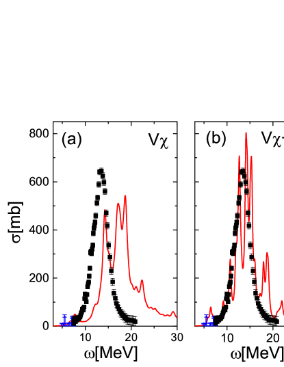
Figure 1: (Color online) TDA $E1$ cross section in ²⁰⁸Pb computed using $V_{\chi}$ (a) only and $V_{\chi}+V_{\rho}$ (b). The experimental data (black squares) are taken from Tamii et al. (2011); Poltoratska et al. (2012); Schwengner et al. (2010); Veyssiere et al. (1970); Schelhaas et al. (1988).

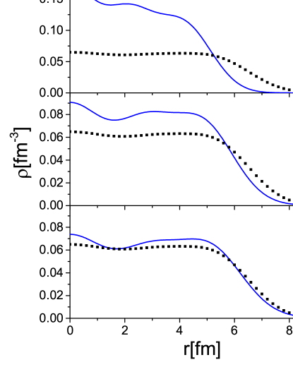
Figure 2: (Color online) Comparison with experiments De Vries et al. (1987) of the HF charge densities obtained by using for the strength of $V_{\rho}$ the values (a) $C_{\rho}=0$, (b) $C_{\rho}=2000$ MeV fm⁶, (c) $C_{\rho}=3000$ MeV fm⁶

IV Calculations and results

IV.1 Dipole response

Our main goal is to compute the $E1$ reduced strength

$$B_{\nu}(E\lambda=1)=\left|\langle\nu\parallel{\cal M}(E\lambda=1)\parallel 0^{+}\rangle\right|^{2},$$ (37)

where

$${\cal M}(E\lambda\mu)=\frac{e}{2}\sum_{i=1}^{A}(1-\tau_{3}^{i})r^{\lambda}_{i}Y_{\lambda\mu}(\hat{r_{i}})$$ (38)

is the electric multipole operator written as the sum of its isoscalar and isovector components, with $\tau_{3}=1$ for neutrons and $\tau_{3}=-1$ for protons.

By inserting the wave functions (24) up to two phonons into the formula (26) and making use of Eq. (II), we get for the $\lambda=1$ transitions from the ground to the $1^{-}$ states

$$<\nu\parallel{\cal M}(E\lambda)\parallel 0^{+}>={\cal C}^{(0^{+})}_{0}\sum_{\beta_{1}}{\cal C}^{(\nu)}_{\beta_{1}}{\cal M}_{\lambda}(0^{+}\rightarrow\beta_{1})$$

$$+(-)^{\lambda}[\lambda]^{-1/2}\sum_{x}{\cal M}_{\lambda}(0^{+}\rightarrow x)Y_{x\lambda}(0^{+}\rightarrow\nu)$$

$$+[\lambda]^{-1/2}\sum_{\alpha_{2}\beta_{2}}{\cal C}^{(0^{+})}_{\alpha_{2}}{\cal C}^{(\nu\lambda)}_{\beta_{2}}{\cal M}_{\alpha_{2}\beta_{2}}(\lambda)$$ (39)

where $\alpha_{n}=(n\alpha)$ and $\beta_{n}=(n\beta)$ label the $n$-phonon components $\mid n\alpha\rangle$ and $\mid n\beta\rangle$ of the ground $\Psi^{0^{+}}_{g}$ and final $1^{-}$ states $\Psi_{\nu}$, respectively. The quantity ${\cal M}_{\lambda}(0^{+}\rightarrow\beta_{1})$ is the TDA amplitude (II) of the transition to the one-phonon component $\mid\beta_{1}\lambda\rangle$ of the final state $\Psi_{\nu}$ and

$$Y_{x\lambda}(0^{+}\rightarrow\nu)=\sum_{\alpha_{2}\beta_{1}}{\cal C}^{(0^{+})}_{\alpha_{2}}{\cal C}^{(\nu)}_{\beta_{1}}X^{(\alpha_{2})}_{(x\lambda)(\beta_{1}\lambda)},$$ (40)

where $X^{(\alpha_{2})}_{(x\lambda)(\beta_{1}\lambda)}=\langle\alpha_{2},0^{+}\parallel O^{\dagger}_{x\lambda}\parallel\beta_{1}\lambda\rangle$.

The first term is dominant. The second may affect transitions involving $1^{-}$ and ground states having sizable one-phonon and two-phonon components, respectively, while the third may contribute to the transitions connecting states both having appreciable two-phonon components.

We will compute the amplitudes defined above, by using the EMPM correlated as well as the unperturbed HF ground state. In this latter case, the formula becomes simply

$$<\nu\parallel{\cal M}(E\lambda)\parallel 0^{+}>=\sum_{\beta_{1}}{\cal C}^{(\nu)}_{\beta_{1}}{\cal M}_{\lambda}(0^{+}\rightarrow\beta_{1}).$$ (41)

The $B_{\nu}(E1)$ strength is used to determine the dipole cross section

$$\sigma=\int_{0}^{\infty}\sigma(\omega)d\omega=\frac{16\pi^{3}}{9\hbar c}\int_{0}^{\infty}\omega{\cal S}(E1,\omega)d\omega$$ (42)

where ${\cal S}(E1,\omega)$ is the $\lambda=1$ strength function

$${\cal S}(E\lambda,\omega)=\sum_{\nu}B_{\nu}(E\lambda)\,\delta(\omega-\omega_{\nu})$$

$$\approx\sum_{\nu}B_{\nu}(E\lambda)\,\rho_{\Delta}(\omega-\omega_{\nu}).$$ (43)

Here $\omega$ is the energy variable, $\omega_{\nu}$ the energy of the transition of multipolarity $E\lambda$ from the ground to the $\nu_{th}$ excited state of spin $J=\lambda$ and

$$\rho_{\Delta}(\omega-\omega_{\nu})=\frac{\Delta}{2\pi}\frac{1}{(\omega-\omega_{\nu})^{2}+(\frac{\Delta}{2})^{2}}$$ (44)

is a Lorentzian of width $\Delta$, which replaces the $\delta$ function as a weight of the reduced strength.

After integration, the cross section becomes

$$\sigma=\frac{16\pi^{3}}{9\hbar c}m_{1},$$ (45)

where

$$m_{1}=\sum_{\nu}\omega_{\nu}B_{\nu}(E1)$$ (46)

is the first moment. If one neglects momentum dependent and exchange terms in the Hamiltonian, $m_{1}$ fulfills the classical energy weighted Thomas-Reiche-Kuhn (TRK) sum rule

$$m_{1}=\frac{\hbar^{2}}{2m}\frac{9}{4\pi}\frac{NZ}{A}e^{2}$$ (47)

and the total cross section assumes the value

$$\sigma=(2\pi)^{2}\frac{\hbar^{2}}{2m}\frac{e^{2}}{\hbar c}\frac{NZ}{A}=60\frac{NZ}{A}({\rm MeV}{\rm mb}).$$ (48)

An observable sensitive to the low-energy spectrum is the dipole polarizability Reinhard and Nazarewicz (2010); Piekarewicz (2011)

$$\alpha_{D}=\frac{8\pi}{9}m_{-1},$$ (49)

where

$$m_{-1}=\sum_{n}\omega^{-1}_{\nu}B_{\nu}(E1)$$ (50)

is the $E1$ inverse moment. This quantity links the dipole polarizability to the cross section $\sigma(\omega)$ according to the relation Tamii et al. (2011)

$$\alpha_{D}=\frac{\hbar c}{2\pi^{2}e^{2}}\int_{0}^{\infty}\omega^{-2}\sigma(\omega)d\omega.$$ (51)

IV.2 Hartree-Fock and TDA

The HF basis is generated in a configuration space which includes 13 harmonic oscillator major shells, up to the principal quantum number $N_{max}=12$. This space is sufficient for reaching a good convergence of the single particle spectra below and around the Fermi surface. In going, for instance, from $N_{max}=9$ to $N_{max}=12$, step by step, the energies change at most by $\sim 0.1$ MeV at each step. More appreciable variations with $N_{max}$ are noticed in the spectrum far above the Fermi surface, a general feature of HF. They, however, induce some fluctuations only in the high energy sector of the TDA strength distribution, which are wiped out by the coupling with the two-phonon states. The low-energy dipole spectrum reaches convergence very fast even at the TDA level. The rate of convergence for both HF and TDA is the same whether we add or not $V_{\rho}$ to $V_{\chi}$.

We have generated the TDA phonons $\mid\lambda\rangle$ in a space which encompasses three major shells above and only one major shell below the Fermi surface. We have checked that this is the minimal space needed to get solutions very close to the ones resulting from diagonalizing the Hamiltonian in the full HF space.

Though $V_{\chi}$ yields considerably more compressed HF spectra Knapp et al. (2014) compared to other potentials Bianco et al. (2014); Hergert et al. (2011), the gap between major shells remains too large with respect to the empirical single particle levels. Due to this large gap, the TDA dipole cross section gets peaked $\sim 7$ MeV above the experimental peak (Figure 1). The two peaks almost overlap once we add $V_{\rho}$ with a coupling constant $C_{\rho}\sim 2000$ MeV $fm^{6}$.

The use of $V=V_{\chi}+V_{\rho}$ improves considerably also the agreement between the HF and the measured nuclear charge density distribution (Figure 2). The sensitivity to $V_{\rho}$ is to be noticed. The empirical charge distribution is reproduced fairly well for $C_{\rho}\sim 3000$ MeV $fm^{6}$. It is, however, more appropriate to use a smaller value since additional diffuseness of the Fermi surface is to be expected from the ground state correlations. We, thus, keep the value $C_{\rho}\sim 2000$ MeV $fm^{6}$ suggested by the dipole response.

It must be stressed once again that, as shown in Ref. Knapp et al. (2014), the HF spectrum so obtained still differs significantly from the empirical one. The consequences of this discrepancy on the dipole strength distribution will be discussed later.

IV.3 EMPM

The two-phonon basis states $\mid(n=2)\beta\rangle$ are generated in a truncated space spanned by the states $\mid(\lambda_{1}\times\lambda_{2})^{\beta}\rangle\equiv\Bigl{\{}O^{\dagger}_{\lambda_{1}}\times\mid\lambda_{2}>\Bigr{\}}^{\beta}$ composed of all TDA phonons, of both parities and of all multipolarities, with dominant $1\hbar\omega$ particle-hole components and, in addition, all two-phonon states with $E_{\lambda_{1}}+E_{\lambda_{2}}\lesssim 20$ MeV and $E_{\lambda_{i}}\lesssim 15MeV$.

This restricted set is used to construct and diagonalize the Hamiltonian matrix. After the Cholesky treatment, we obtain a truncated basis of $\sim$2.500 and $\sim$6.000 correlated orthonormal states $\mid(n=2)\beta,0^{+}\rangle$ and $\mid(n=2)\beta,1^{-}\rangle$, respectively.

No significant changes in the spectrum are produced if the number of TDA phonons is increased. We have raised the acceptance limit up to 30 MeV ($E_{\lambda_{1}}+E_{\lambda_{2}}\lesssim 30$ MeV) thereby generating $\sim$9.000 and $\sim$22.000 $\mid(n=2)\beta,0^{+}\rangle$ and $\mid(n=2)\beta,1^{-}\rangle$ states, respectively. We found that the low-lying energy peaks are shifted downward by only $\sim 0.2$ MeV and the strength distribution is little affected.

The correlated $\mid(n=2)\beta\rangle$ states are added to the unperturbed ground state plus the TDA one-phonon basis to diagonalize the residual Hamiltonian and determine the ground and $1^{-}$ EMPM states.

Due to the two-phonon coupling, the ground state gets depressed by $\Delta E=7.3$ MeV with respect to the unperturbed HF state and becomes strongly correlated. Its two-phonon components account for $\sim 24\%$ of the wavefunction, in analogy with previous results obtained for ¹⁶O Bianco et al. (2012a), the same ²⁰⁸Pb Bianco et al. (2012b) and ¹³²Sn Knapp et al. (2014) and, also, consistently with shell model calculations on ²⁰⁸Pb Schwengner et al. (2007); Brown (2000).

This ground state energy shift would spoil the description of the dipole response by pushing the strength at too high energy, unless we add the three-phonon basis states to determine the $1^{-}$ eigenstates. It is in fact known from EMPM calculations on ¹⁶O Bianco et al. (2012a) that the three-phonon configurations couple strongly to the $1^{-}$ TDA phonons and, thereby, counterbalance the coupling between ground and two-phonon states by pushing the strength back to the experimental region.

Including the three-phonon basis in a heavy nucleus like ²⁰⁸Pb is too time consuming, without drastic and uncontrollable truncations and approximations. Thus, we confine ourselves to a two-phonon space and, for consistency, refer the energies to the unperturbed HF ground state. This assumption, implicit in all extensions of RPA, was already made in shell model calculations Schwengner et al. (2007); Brown (2000) as well as in our previous EPMP calculations Bianco et al. (2012b); Knapp et al. (2014).

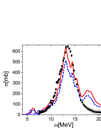
Figure 3: (Color online) Experimental Tamii et al. (2011); Poltoratska et al. (2012); Schwengner et al. (2010); Veyssiere et al. (1970); Schelhaas et al. (1988) versus EMPM $E1$ cross sections in ²⁰⁸Pb. A Lorentzian of width $\Delta=0.5$ MeV was adopted. The EMPM cross section is computed using a HF (continuous red line) and a correlated (dashed blue line) ground states.

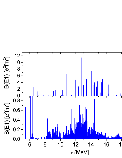
Figure 4: (Color online) TDA (a) versus EMPM (b) $E1$ strength distributions in ²⁰⁸Pb. The different scales used for the two-plots are to be noticed.

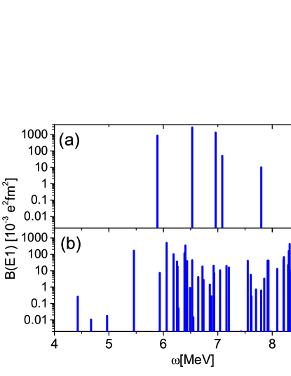
Figure 5: (Color online) TDA (a) versus EMPM (b) $E1$ low-lying spectra plotted on an amplified (logarithmic) scale.

Figure 6: (Color online) EMPM versus experimental $E1$ low-lying spectra. The EMPM spectra are compute with (a) and without (b) ground state correlations. The experimental data (c) are taken from Poltoratska et al. (2012).

Both correlated and HF ground states are used, in alternative, to compute the EMPM cross section. The two theoretical quantities are compared with the experimental data in Figure 3. With respect to TDA, shown in Figure 1, the two EMPM cross sections are quenched and follow roughly the smooth trend of the measured cross section.

The data are better reproduced if the unperturbed HF ground state $\mid 0\rangle$ is used, while the correlations induce a too pronounced damping. In fact, in the HF case, the transition amplitude is simply given by the term (41) which couples $\mid 0\rangle$ to the one-phonon components of the $1^{-}$ states. When the correlated ground state is used, this term, though remaining dominant, is multiplied by the amplitude coefficient ${\cal C}^{(0^{+})}_{0}$ of the HF component ( Eq.(IV.1)), which is of the order $|{\cal C}^{(0^{+})}_{0}|\sim 0.8$.

Such a quenching factor should be counterbalanced by a corresponding overall enhancement of the amplitudes of the one-phonon components. This, however, is promoted by the coupling to the three-phonon subspace, not included here. The conclusion to be drawn is that, in the absence of three phonons, the transition strengths should be computed by adopting the unperturbed HF ground state consistently with the assumption made for the energy levels. Both assumptions are tacitly made in all extensions of RPA.

The calculation yields a secondary peak around $\sim 17$ MeV not observed experimentally. Such an unwanted peak does not appear in other microscopic multiphonon calculations like the one carried out in QPM Bertulani and Ponomarev (1999) and may be an effect of the mentioned discrepancies between HF and empirical single particle energies.

The overall strength as well as the energy weighted sum $m_{1}$ remain practically unchanged in going from TDA to the EMPM if the HF ground state is adopted. In both cases, the momentum $m_{1}$ overestimates the Thomas-Reiche-Kuhn (TRK) sum rule by a factor $\sim 1.7$. This factor would be reduced by washing out the unwanted secondary high-energy peak. Once again, the HF energies come into play.

Quenching and smoothness of the cross section are a consequence of the fragmentation of the strength which enhances enormously the density of levels and shortens the TDA peaks. As shown in Figure 4, pronounced transitions occur at low energy in both TDA and EMPM. They are responsible for the low-lying bump in the cross section (Figure 3). The EMPM spectrum is extremely rich compared to TDA and is composed of shorter peaks (Figure 5). The quenching is considerably more pronounced when the ground state correlations are included.

In both cases, the calculation reproduces only qualitatively the experimental strength distribution. A detailed comparison (Figure 6) shows that significant discrepancies exist. Some EMPM transitions result to be either too strong or too weak compared to the measured ones. The calculation, for instance, yields about 20 $1^{-}$ levels between $\sim 4.5$ MeV and $\sim 7$ MeV, twice as much as the levels detected experimentally Tamii et al. (2011); Poltoratska et al. (2012). The large majority of them, however, carry strengths which are either negligible or of the order $10^{-2}$ $e^{2}fm^{2}$.

Most of the strength remains concentrated in three states. The transition at $\simeq 5.46$ MeV has a strength close to the one measured for the level at $5.51$ MeV. The other two, at $\simeq 6.06$ MeV and $\simeq 6.40$ MeV, do not have experimental counterparts. As shown in Table 1, these three states have basically a one-phonon character. Apparently they are little affected by the phonon coupling, which is, instead, very effective in the higher energy regions.

In any case, one can infer from a comparison with Figure 6 of Ref. Poltoratska et al. (2012) that our computed spectrum is comparable with the ones computed in QPM and RTBA and, especially, with the spectrum obtained in shell model by using empirical single particle energies and a phenomenological potential in a restricted configuration space Schwengner et al. (2010).

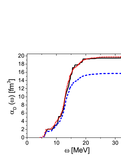
Figure 7: (Color online) Polarizability as function of energy. The EMPM calculation is carried out using a HF (red line) and a correlated ground state (black line).

It is of great interest to compute the dipole polarizability $\alpha_{D}$ (51). If the HF ground state is used, we obtain $\alpha_{D}\simeq 19.78$ $fm^{3}$, very close to the value $\alpha_{D}=20.1\pm 0.6$ fm³ determined experimentally, once all the data up to 130 MeV are included Tamii et al. (2011). Apparently, the phonon coupling does not affect the polarizability. This gets quenched, instead, if the ground state correlations are included and assumes the smaller value $\alpha_{D}\simeq 15.71$ $fm^{3}$.

As shown in Figure 7, $\alpha_{D}(\omega)$ rises sharply in correspondence of the PDR and the GDR regions, indicating that it is determined almost exclusively by these two resonances.

The dipole polarizability has been shown Reinhard and Nazarewicz (2010) to be closely correlated to the excess neutron radius

$$\Delta r_{np}=\sqrt{<r_{n}^{2}>}-\sqrt{<r_{p}^{2}>}.$$ (52)

This was actually extracted from the measured $\alpha_{D}$ in ²⁰⁸Pb by exploiting such a correlation Tamii et al. (2011).

We have computed the neutron skin radius using both HF and correlated ground states (24). The EMPM yields for the proton ($\tau=p)$ and neutron ($\tau=n$) mean square radii the expression

$$\langle r_{\tau}^{2}\rangle=\langle\Psi_{0}\mid r^{2}_{\tau}\mid\Psi_{0}\rangle=\langle r^{2}_{\tau}\rangle_{HF}+\langle r^{2}_{\tau}\rangle_{corr},$$ (53)

where $\langle r^{2}_{\tau}\rangle_{HF}$ is the HF value and $\langle r^{2}_{\tau}\rangle_{corr}$ is the contribution coming from the two-phonon components. This is given by

$$\langle r^{2}_{\tau}\rangle_{corr}=\sum_{\alpha\beta}\delta_{J_{\alpha}J_{\beta}}\delta_{J_{\alpha}0}{\cal C}^{(0)}_{\alpha}{\cal C}^{(0)}_{\beta}{\cal M}_{\alpha\beta}^{(0)},$$ (54)

where

$${\cal M}_{\alpha\beta}^{(0)}=\sum_{rs}\langle r\parallel r^{2}_{\tau}\parallel s\rangle\langle\beta\parallel(a^{\dagger}_{r}\times b_{s})^{0}\parallel\alpha\rangle.$$ (55)

The HF proton radius is $r^{(HF)}_{p}=5.06$ fm, smaller than the experimental value $r_{p}^{(exp)}\simeq 5.45$ fm. The neutron radius is estimated to be $r^{(HF)}_{n}=5.28$ fm. We, thus, obtain for the neutron skin $\Delta r_{np}=0.22$ fm, which is in the range of the values determined experimentally Tamii et al. (2011); Abrahamyan et al. (2012); Tarbert et al. (2014).

If the ground state correlations are taken into account, the proton radius raises to $r_{p}=5.19$ fm, not enough to reach the measured value. On the other hand, this estimate was computed in a truncated two-phonon space and, therefore, is to be considered a lower limit. An enlargement of the space would increment further the radius.

The neutron radius raises from $r^{(HF)}_{n}=5.28$ fm to $r_{n}=5.5$ fm. It follows that the neutron excess radius goes from the $\Delta r^{(HF)}_{np}=0.22$ fm to $\Delta r_{np}=0.31$ fm, which approaches the upper limit of the range of values deduced from experiments Abrahamyan et al. (2012).

Like the density distribution (Figure 2), the radii are quite sensitive to the strength $C_{\rho}$ of the density dependent potential $V_{\rho}$. As shown in Figure 8, the neutron excess radius decreases as $C_{\rho}$ increases. It would therefore be easy to reduce or enhance such a quantity by a modest increment (decrement) of such a strength.

Figure 8: Neutron skin thickness versus the strength of $V_{\rho}$.

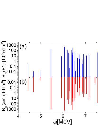
Figure 9: (Color online) EMPM isovector (a) versus isoscalar (b) dipole low-lying spectra plotted on a logarithm scale so as to make clearly visible the many small peaks not discernible otherwise. The isovector strength is nothing but the low-lying sector of the spectrum shown in Figure 4(b). The isoscalar one is obtained by using the isoscalar operator (56).

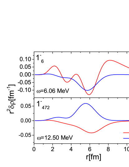
Figure 10: (Color online) $E1$ transition density for a low-lying $1^{-}$ state (a) and one in the GDR region (b).

Table 1: Phonon composition of the lowest twenty $1^{-}$ states

$J^{\pi}_{\nu}$		$\omega_{\nu}$ (MeV)		$|C^{(\nu)}_{1}|^{2}$		$|C^{(\nu)}_{2}|^{2}$
$1^{-}_{1}$		4.42780		0.00017		0.99983
$1^{-}_{2}$		4.67271		0.00083		0.99917
$1^{-}_{3}$		4.96609		0.00014		0.99986
$1^{-}_{4}$		5.46012		0.95558		0.04442
$1^{-}_{5}$		5.93408		0.03132		0.96868
$1^{-}_{6}$		6.05979		0.90712		0.09288
$1^{-}_{7}$		6.18594		0.05422		0.94578
$1^{-}_{8}$		6.25179		0.04936		0.95064
$1^{-}_{9}$		6.26285		0.05409		0.94591
$1^{-}_{10}$		6.27701		0.00310		0.99690
$1^{-}_{11}$		6.38869		0.15931		0.84069
$1^{-}_{12}$		6.40474		0.69907		0.30093
$1^{-}_{13}$		6.42531		0.03371		0.96629
$1^{-}_{14}$		6.43502		0.03215		0.96785
$1^{-}_{15}$		6.48971		0.86985		0.13015
$1^{-}_{16}$		6.53002		0.00956		0.99044
$1^{-}_{17}$		6.55127		0.00485		0.99515
$1^{-}_{18}$		6.64103		0.00346		0.99654
$1^{-}_{19}$		6.71925		0.01301		0.98699
$1^{-}_{20}$		6.73778		0.00058		0.99942

Table 2: Particle-hole composition of two selected phonons

$1^{-}$	$\omega=5.890MeV$
$(p(h)^{-1})^{\pi}$	$C_{ph}^{\pi}$	$(p(h)^{-1})^{\nu}$	$C_{ph}^{\nu}$
$0h_{9/2}(0g_{7/2})^{-1}$	-0.05221	$0i_{11/2}(0h_{9/2})^{-1}$	0.05390
$1f_{7/2}(1d_{5/2})^{-1}$	-0.03103	$1g_{9/2}(1f_{7/2})^{-1}$	-0.05141
$1f_{5/2}(1d_{3/2})^{-1}$	-0.02924	$2d_{5/2}(1f_{7/2})^{-1}$	0.01384
$2p_{3/2}(1d_{5/2})^{-1}$	0.01366	$2d_{5/2}(2p_{3/2})^{-1}$	-0.04462
$2p_{1/2}(1d_{3/2})^{-1}$	0.01046	$3s_{1/2}(2p_{3/2})^{-1}$	0.15998
$2p_{1/2}(2s_{1/2})^{-1}$	-0.01926	$3s_{1/2}(2p_{1/2})^{-1}$	0.97117
$0i_{13/2}(0h_{11/2})^{-1}$	-0.06687	$2d_{3/2}(2p_{3/2})^{-1}$	-0.02626
		$2d_{3/2}(2p_{1/2})^{-1}$	0.06317
		$1g_{7/2}(1f_{5/2})^{-1}$	-0.03117
		$0j_{15/2}(0i_{13/2})^{-1}$	0.08284
		$2g_{9/2}(1f_{7/2})^{-1}$	0.01165
		$3d_{5/2}(2p_{3/2})^{-1}$	0.01132
		$4s_{1/2}(2p_{3/2})^{-1}$	-0.01727
		$2g_{7/2}(1f_{5/2})^{-1}$	0.01277
$1^{-}$	$\omega=12.816MeV$
$0h_{9/2}(0g_{9/2})^{-1}$	-0.11797	$0i_{11/2}(0h_{9/2})^{-1}$	-0.12090
$0h_{9/2}(0g_{7/2})^{-1}$	-0.09381	$1g_{9/2}(0h_{9/2})^{-1}$	0.08459
$1f_{7/2}(0g_{7/2})^{-1}$	-0.03875	$1g_{9/2}(1f_{7/2})^{-1}$	-0.21304
$1f_{7/2}(1d_{5/2})^{-1}$	0.07336	$2d_{5/2}(1f_{7/2})^{-1}$	0.01687
$1f_{5/2}(0g_{7/2})^{-1}$	-0.03795	$2d_{5/2}(1f_{5/2})^{-1}$	-0.02538
$1f_{5/2}(1d_{5/2})^{-1}$	-0.09910	$2d_{5/2}(2p_{3/2})^{-1}$	-0.03684
$1f_{5/2}(1d_{3/2})^{-1}$	0.04318	$3s_{1/2}(2p_{1/2})^{-1}$	-0.01597
$2p_{3/2}(1d_{3/2})^{-1}$	0.17526	$2d_{3/2}(1f_{5/2})^{-1}$	-0.03881
$2p_{3/2}(2s_{1/2})^{-1}$	0.02467	$2d_{3/2}(2p_{3/2})^{-1}$	-0.03722
$2p_{1/2}(1d_{3/2})^{-1}$	-0.17532	$2d_{3/2}(2p_{1/2})^{-1}$	0.01313
$0i_{13/2}(0h_{11/2})^{-1}$	0.46993	$1g_{7/2}(0h_{9/2})^{-1}$	0.04067
$1g_{9/2}(0h_{11/2})^{-1}$	-0.01005	$1g_{7/2}(1f_{7/2})^{-1}$	-0.57127
$0i_{11/2}(0h_{11/2})^{-1}$	-0.06708	$1g_{7/2}(1f_{5/2})^{-1}$	0.03749
$3p_{3/2}(1d_{3/2})^{-1}$	0.01351	$0j_{15/2}(0i_{13/2})^{-1}$	0.45810
$3p_{3/2}(2s_{1/2})^{-1}$	0.01245	$1h_{11/2}(0i_{13/2})^{-1}$	-0.01488
		$2g_{9/2}(1f_{7/2})^{-1}$	-0.05808
		$3d_{5/2}(1f_{5/2})^{-1}$	-0.03141
		$3d_{5/2}(2p_{3/2})^{-1}$	-0.08047
		$4s_{1/2}(2p_{1/2})^{-1}$	-0.06666
		$3d_{3/2}(1f_{5/2})^{-1}$	-0.04485
		$3d_{3/2}(2p_{3/2})^{-1}$	-0.05249
		$3d_{3/2}(2p_{1/2})^{-1}$	0.02462
		$2g_{7/2}(0h_{9/2})^{-1}$	-0.01030
		$2g_{7/2}(1f_{7/2})^{-1}$	-0.05356
		$0j_{13/2}(0i_{13/2})^{-1}$	-0.18118

For a more complete investigation of the nature of the low-lying $E1$ levels, we compute also the isoscalar dipole transition strength using the operator

$${\cal M}_{IS}(\lambda=1,\mu)=\sum_{i=1}^{A}r_{i}^{3}Y_{1\mu}(\hat{r_{i}}).$$ (56)

The computed isoscalar and isovector spectra overlap over the entire low-energy region (Figure 9), in perfect analogy with the equivalent calculation performed for ¹³²Sn Knapp et al. (2014).

This prediction seems to be disproved by the isoscalar-isovector splitting observed in $(\alpha,\alpha^{\prime}\gamma)$ experiments on open shell nuclei like ¹⁴⁰Ce Savran et al. (2006) and ¹²⁴Sn Govaert et al. (1998); Endres et al. (2010, 2012). For a conclusive test, it would be of great help to perform an analogous experiment on the stable doubly magic ²⁰⁸Pb.

Our theoretical results suggests that these low-lying transitions are promoted mainly by the excitations of the neutrons above the N=Z core thereby hinting at their pygmy nature.

Such a hint is confirmed by the behavior of the transition densities, shown in Figure 10. The low-lying transition density shows a neutron excess for large values of the radial coordinate. This behavior is to be contrasted with the one exhibited by the transition to the most strongly excited $1^{-}$ state in the region of the GDR, which clearly describes an oscillation of protons versus neutrons.

A further support comes from the investigation of the structure of the wave functions. As shown in Table 1, the most strongly excited low-lying states have an overwhelming one-phonon component. The large majority of the weakly excited states, instead, have a dominant two-phonon structure.

Table 2 shows the p-h composition of two typical phonons contributing to the strength in the low-energy and GDR regions, respectively. They have distinctive structures. The low-lying phonon is composed predominantly of p-h neutron excitations above the $N=Z$ core, with a very dominant single p-h neutron configuration. The phonon in the GDR region is built of both proton and neutron p-h configurations of comparable amplitudes in opposition of phase.

V Concluding remarks

The inclusion of a subset of the two-phonon basis states in the selfconsistent EMPM calculation fragments strongly the dipole strength computed in TDA by greatly enhancing the density of levels.

It is, however, necessary to assume an unperturbed HF ground state in order to reproduce with fairly good accuracy the GDR in its magnitude and smooth trend and to describe satisfactorily the global properties of the dipole response, described here by the dipole polarizability and the neutron skin radius.

This assumption, which underlies all extensions of RPA, has a theoretical justification. Since the HF ground state couples strongly to the two-phonon basis, it is necessary to include the three-phonon states in order to obtain a comparable effect on the $1^{-}$ one-phonon states. Consistency requires that the two-phonon correlations in the ground state should be neglected if the three-phonon basis is missing.

The ultimate goal is to enlarge the space so as to include such a basis. The coupling of the three-phonons to the other subspaces is expected to modify the weight of the one and two phonon components of the total $1^{-}$ wave functions and, therefore, should affect the strength distribution. Whether such a redistribution leads to a better agreement with experiments can be ascertained only by explicit calculations. In this perspective, we are trying to improve the efficiency of the codes and, concurrently, search for reliable methods for truncating the phonon space.

It is also compelling to improve further the agreement between HF and empirical single particle spectra in order to be able to get an unambiguous correspondence between theoretical and experimental levels, especially in the low-energy region. Such a task can be achieved only by acting on the NN interaction.

Though the optimized chiral potential $V_{\chi}=NNLO_{opt}$Ekström et al. (2013) may represent a promising starting point, higher order terms need to be taken into account. This is done here effectively by adding a phenomenological density dependent potential which simulates a contact three-body force.

Such a potential plays a crucial role. It improves to some extent the description of the single particle levels, enhances the diffuseness of the Fermi surface consistently with experiments, and shifts the dipole spectrum in the region of observation. It is, however, phenomenological and contains an unconstrained coupling constant.

We need, in any case, a more refined potential able to provide a more accurate and detailed description of the single particle spectra. The new optimized interaction $NNLO_{sat}$ Ekström et al. (2015), involving both two- and three-body components of NNLO, is a possible candidate.

A calculation based on such a potential would be parameter free and would link the dipole spectra directly and exclusively to the NN interaction. If carried out in a space encompassing up to three phonons, it would represent an additional reliable test for the chiral interaction.