Trusted frequency region of convergence for the enclosure method in an inverse heat equation

Abstract

This paper is concerned with the numerical implementation of a formula in the enclosure method as applied to a prototype inverse initial boundary value problem for thermal imaging in a one-space dimension. A precise error estimate of the formula is given and the effect on the discretization of the used integral of the measured data in the formula is studied. The formula requires a large frequency to converge; however, the number of time interval divisions grows exponetially as the frequency increases. Therefore, for a given number of divisions, we fixed the trusted frequency region of convergence with some given error bound. The trusted frequency region is computed theoretically using theorems provided in this paper and is numerically implemented for various cases. AMS: 35R30

KEYWORDS: enclosure method, inverse initial boundary value problem, heat equation, thermal imaging

1 Introduction

Thermal imaging is described as follows: given a heat flux on the surface of an object and a measured surface temperature, determine the internal thermal properties of the object or the shape of some unknown inaccessible portion of the boundary [2].

$$\left\{\begin{array}[]{ll}\displaystyle u_{t}=\triangle u&\text{in}\,\Omega\times{\mathbb{R}^{+}},\\ \\ \displaystyle\frac{\partial u}{\partial n}=f&\text{on}\,\partial\Omega\times{\mathbb{R}^{+}},\\ \\ \displaystyle u(x,0)=u_{0}(x)&\text{on}\,\Omega\times\{t=0\}.\end{array}\right.$$

Let the support of $f$ and the measurement set be contained in the known boundary $\Gamma\subset\partial\Omega$ . Thermal imaging is redescribed as determining the part of $\partial\Omega$ such that $f=0$, which means a perfectly insulating boundary. The problem is applied to identify back surface corrosion and damage, such as the use of infrared thermography to find burn injuries and the selection of donor sites for skin grafts.

It is reported in [2] that if

$$\left\{\begin{array}[]{l}\displaystyle\Omega_{1}=[0,2\pi]\times[0,\pi],\\ \\ \displaystyle\Omega_{2}=\Omega_{1}\setminus\left[\frac{2\pi}{3},\frac{4\pi}{3}\right]\times\left[0,\frac{2\pi}{3}\right],\\ \\ \displaystyle u(t,x,y)=e^{-\frac{9}{2}t}\cos\left(\frac{3}{2}x\right)\cos\left(\frac{3}{2}y\right),\\ \\ \displaystyle\Gamma=[0,2\pi]\times[y=\pi],\end{array}\right.$$

$\Omega_{1}\setminus\Gamma$ and $\Omega_{2}\setminus\Gamma$ are two different unknown boundaries on which the Neumann data $f$ vanishes. This is an example of the nonuniqueness of the thermal imaging problem.

On the other hand, two uniqueness results are also reported in [2].

• If $u_{0}$ is constant and $u_{1}=u_{2}$ on $\Gamma\times(0,T)$, then we have $\Omega_{1}=\Omega_{2}$ and $u_{1}=u_{2}$.

• If $u_{0}$ is nonconstant, special conditions are required for the uniqueness of $\Omega$ and $u$. That is, if

  $$\|f(t,\cdot)\|_{L^{2}(\partial\Omega)},\|f_{t}(t,\cdot)\|_{L^{2}(\partial\Omega)}<\infty,\int_{\partial\Omega}f(t,x)dS_{x}>G_{0}>0,$$

  then $u_{1}=u_{2}$ on $\Gamma\times(0,\infty)$ implies $\Omega_{1}=\Omega_{2}$ and $u_{1}=u_{2}$.

A boundary element method is presented for a linearised inverse problem of (1.1), as a numerical method [3]. On the other hand, in this paper, the enclousre method is used for the nonlinear inverse problem of (1.1).

In [7], some inverse problems for the heat and wave equations were included in a one-space dimension, and the first author introduced the enclosure method in a time domain. The enclosure method is an analytical method which has its origins in [6] and [8]. Therein, the governing equations are elliptic equations and the observation data are given by a single set of Cauchy data and the Dirichlet-to-Neumann map, respectively. The enclosure method developed in [7] can be considered as an extension of the concept in [6] to include inverse problems in the time domain. See also [9, 10, 11, 12, 13].

It is reported that the numerical implementation of thermal imaging without any linearisation as in [3] even in one -space dimensional case is not trivial [4]. Let us consider the following one-dimensional thermal imaging problem with constant initial data.

Let $0<a<\infty$ and $0<T<\infty$. Given $f\in L^{2}(0,\,T)$ let $u$ be a solution of the problem:

$$\left\{\begin{array}[]{ll}\displaystyle u_{t}=u_{xx}&\text{in}\,\,]0,\,a[\times\,]0,\,T[,\\ \\ \displaystyle u_{x}(a,t)=0&\text{for}\,t\in\,]0,\,T[,\\ \\ \displaystyle u_{x}(0,t)=f(t)&\text{for}\,t\in\,]0,\,T[,\\ \\ \displaystyle u(x,0)=0&\text{in}\,]0,\,a[.\end{array}\right.$$

Note that, because the initial data is constant, we can choose any nonzero Neumann data $f$ for the uniqueness of the unknown perfect conducting boundary $a$: However, we impose some weak condition (1.4) for $f$ for the enclosure method to be valid. The solution class is the same as that in [7, 11] which was obtained from [5].

Let $\tau>0$ and

$$v(x,t)=e^{-\tau^{2}t}e^{-x\tau}.$$

This $v$ satisfies the backward heat equation $v_{t}+v_{xx}=0$ in $]0,\,\infty[\times\,]0,\,T[$.

The so-called indicator function for the enclosure method here takes the form

$$\begin{array}[]{ccl}\displaystyle I(\tau)&=&\int_{0}^{T}\left(u_{x}(0,t)v(0,t)-v_{x}(0,t)u(0,t)\right)dt\\ \\ \displaystyle\hfil&=&\tau\hat{u}(0,\tau)+\hat{f}(\tau)\end{array}$$

where $u$ satisfies (1.2) and $\hat{w}(\tau)=\int_{0}^{T}e^{-\tau^{2}t}w(t)dt$ which is a modified Laplace transform with finite time interval $T$. Let us consider $\tau$ to be the frequency corresponding to the enclosure method.

Assume that there exist positive numbers $C_{\mu}$, $\mu$, and $\tau_{0}$ such that

$$\left|\hat{f}(\tau)\right|\geq C_{\mu}\,\tau^{-\mu},\,\,\forall\tau\geq\tau_{0}.$$

Then, by [7], we have the formula

$$\lim_{\tau\longrightarrow\infty}\frac{1}{-2\tau}\log|I(\tau)|=a.$$

Note that (1.4) is a restriction of the strength of the heat flux at $t=0$ from below. In particular, $f(t)$ cannot be $0$ at $t=0$ with infinite order. It is easy to see that condition (1.4) is satisfied if $f\in L^{2}(0,\,T)$ satisfies one of the following conditions for some $\delta\in\,]0,\,T[$:

$\bullet$ $\exists C>0$ such that $f(t)\geq C$ a.e. in $]0,\,\delta[$.

$\bullet$ $f\in C^{1}([0,\,\delta])$ and $f(0)\not=0$;

$\bullet$ $f\in C^{l+1}([0,\,\delta])$ with $l\geq 1$ and $f^{(s)}(0)=0$ for all $s=0,1,\cdots,l-1$ and $f^{(l)}(0)\not=0$.

When $f(t)=t^{r},r=0,1,2,\cdots$ and $\tau>\frac{1}{\sqrt{T}}$, we have

$$0<C_{\mu}\tau^{\mu}\leq\hat{f}(\tau)\leq r!\tau^{\mu}$$

where

$$\mu=2(r+1),\;\;C_{\mu}=r!\left(1-\frac{\sum_{k=0}^{r}\frac{1}{k!}}{e}\right).$$

(1.5) extracts $a$ from $u(0,t)$ given at a.e. $t\in\,]0,\,T[$ for a fixed known $f$. A naive extraction procedure of $a$ is: just fix a large $\tau$ and compute an approximation of $a$ such as

$$\frac{\log|I(\tau)|}{-2}\approx a\tau.$$

by finding a linear function fitting some values of $\frac{\log|I(\tau)|}{-2}$ at $\tau=\tau_{1},\cdots\,\tau_{m}$ in the least-square sense and compute its slope which will be a candidate for the approximation of $a$. This idea has been introduced in [15] for the enclosure method [8] and tested using an analytical solution of the direct problem. See also [14] for the enclosure method [6]. Therein a similar numerical method has been tested using a solution of the direct problem constructed by finite element method. However, in this paper, rather than using linear approximation, a direct computation will be used with precise error analysis.

In this paper, instead of using (1.5) we develop another formula which is mathemaitcally equivalent . That is,

$$\lim_{\tau\longrightarrow\infty}a(\tau)=a,\;\;$$

where

$$a(\tau)=\frac{1}{-2\tau}\log\left|\frac{I(\tau)}{-2\hat{f}(\tau)}\right|.$$

Note that, since $f\in L^{2}(0,T)$ and satisfies (1.4), we have

$$\lim_{\tau\longrightarrow\infty}\frac{\log|\hat{f}(\tau)|}{\tau}=0.$$

Therefore, (1.5) and (1.7) are mathematically equivalent for $f\in L^{2}(0,T)$ satisfying (1.4).

Then, what is the advantage of using (1.7) rahter than (1.5)? The reason is the following asymptotic formula as $\tau\longrightarrow\infty$:

$$I(\tau)=-2\hat{f}(\tau)e^{-2\tau a}(1+O(\tau^{-1})),$$

$$a(\tau)-a=O(\tau^{-1}).$$

Although the asymptotic convergence (1.8) is covered in [7] for equations that are more general than (1.2), the formula (1.5), instead of (1.7), is used for the numerical approximation; such inconsistant use of a formula makes the numerical scheme have not optimal order of convergence, even if a direct method is used. In this paper, we reprove (1.8), prove the approximation error (1.9), and derive a numerical scheme based on (1.7). That is, we introduce a numerical method based on (1.7) instead of (1.5). This approach would enable us to perform error analysis indicating the convergence order depending on the frequency $\tau$, final time $T$, and the Neumann data $f$, which would not be given when we use (1.5). This is the main reason for constructing the present numerical method based on (1.7), instead of on (1.5). In detail, we could have the following theorem:

Theorem 1.1. Assume that we know two positive constants $a_{L}$ and $a_{U}$ such that

$$a_{L}\leq a\leq a_{U}.$$

Assmume that $f\in L^{\infty}[0,\,T]$. Further, assume that there exists a positive number $\tau_{0}$ such that (1.4) holds for all $\tau\geq\tau_{0}$,

$$\tau_{0}\geq\frac{3a_{U}}{4T}\left(1+\sqrt{1+\frac{8T\mu}{9a_{U}^{2}}}\right),$$

and

$$\frac{e^{-T\tau_{0}^{2}+3a_{U}\tau_{0}}\tau_{0}^{\mu}}{2C_{\mu}}C_{T}\|f\|_{L^{\infty}[0,T]}\leq\epsilon<1,$$

where $C_{T}$ is given in (2.10). Then, for all $\tau\geq\tau_{0}$ we have

$$\begin{array}[]{c}\displaystyle|a(\tau)-a|\leq\frac{-\log(1-e^{-2a_{L}\tau})}{2\tau}+\frac{C_{T}\|f\|_{L^{\infty}[0,T]}}{4C_{\mu}(1-\epsilon)}e^{-T\tau^{2}+3a_{U}\tau}\tau^{\mu-1}\\ \\ \displaystyle\leq\frac{-\log(1-e^{-2a_{L}\tau_{0}})}{2\tau_{0}}+\frac{\epsilon}{2\tau_{0}(1-\epsilon)}.\end{array}$$

Conditions (1.4), (1.10), and (1.11) are the criteria for the choice of $\tau_{0}$ when $a_{U},a_{L},C_{\mu},\mu,C_{T},\|f\|$ are known. This result ensures the accuracy of the approximation $a(\tau)$ exactly for $a$ for all $\tau\geq\tau_{0}$. Thus, the problem becomes that of how to compute $a(\tau)$ as precisely as possible from observation data.

In the computation of $a(\tau)$ in (1.3) and (1.7), we need $u(0,t)$ for all $t\in]0,\,T[$. However, in practice, it is not possible to know $u(0,t)$ for all $t\in]0,\,T[$. Here, we consider how to compute $a(\tau)$ approximately from temperatures $u(t_{j}),t_{j}=\frac{jT}{N_{t}},j=0,\cdots,N_{t}$ equidistantly sampled at $N_{t}$ discrete times taken from time interval $[0,\,T]$.

Let

$$Q_{L}\left(\int_{0}^{T}g(t)dt\right)=\frac{1}{L}\sum_{k=1}^{L-1}g\left(\frac{kT}{L}\right)+\frac{g(0)+g(T)}{2L}$$

denote the trapezoidal rule for the integral of a continuous function $g$ over $[0,\,T]$ with $L$ equidistant subdivision. It is well known (see [1]) that if $g$ is twice continuously differentiable, then the error has the estimate

$$\left|\int_{0}^{T}g(t)dt-Q_{L}\left(\int_{0}^{T}g(t)dt\right)\right|\leq\frac{T^{3}}{12L^{2}}\sup_{0\leq t\leq T}|g^{\prime\prime}(t)|.$$

Therefore, another issue that would have to be considered for the numerical implementation of (1.7) is the effect of the division number $N_{t}$ for the time interval $[0,T]$. When the trapezoidal rule is used for $\hat{u}(\tau)$, it becomes possible to define the following:

$$\left\{\begin{array}[]{l}\displaystyle Q_{N_{t}}(\hat{u}(\tau))=\frac{1}{N_{t}}\sum_{j=1}^{N_{t}-1}e^{\frac{-jT\tau^{2}}{N_{t}}}u(0,\frac{jT}{N_{t}})+\frac{u(0,0)+u(0,T)}{2N_{t}},\\ \\ \displaystyle I_{N_{t}}(\tau)=\tau Q_{N_{t}}(\hat{u}(\tau))+\hat{f}(\tau),\\ \\ \displaystyle a_{N_{t}}(\tau)=\frac{1}{-2\tau}\log\left|\frac{I_{N_{t}}(\tau)}{-2\hat{f}(\tau)}\right|.\end{array}\right.$$

As the error (1.13) of the trapezoidal rule $Q_{N_{t}}(\hat{u}(\tau))$ depends on $\frac{1}{N_{t}^{2}}$ and $\tau^{4}$, because of the second derivative of $e^{-\tau^{2}t}u(0,t)$, the resulting error between $a$ and the approximation $a_{N_{t}}(\tau)$ is proportional to $N_{t}^{-2}$ and $e^{2a\tau}\tau^{4}$. Therefore, for the approximation $a_{N_{t}}(\tau)$ to converge to $a$, it is required that $N_{t}$ is proportional to $e^{a\tau}\tau^{\frac{5+\mu}{2}+\delta}$ for a relatively large $\tau$ with some positive $\delta$ by the following Theorem 1.2, resulting in a numerically very expensive method. Remind that the norm for the Sobolev space $W^{2,\infty}[0,T]$ is defined by

$$\|f\|_{W^{2,\infty}[0,T]}=\max_{0\leq s\leq T}(|f(s)|,|f_{t}(s)|,|f_{tt}(s)|).$$

Theorem 1.2. Under the conditions of Theorem 1.1, we further assume that $f\in W^{2,\infty}[0,\,T],\;f(0)=f^{\prime}(0)=0$ and $\tau_{0}$ also satisfies

$$\frac{T^{3}C_{\max}\|f\|_{W^{2,\infty}[0,T]}}{24C_{\mu}(1-\epsilon)}\left(\frac{1}{\tau_{0}^{\delta}}+\frac{1}{\tau_{0}^{2+\delta}}\right)^{2}\leq\eta<1,$$

where $C_{max}$ is given in (2.3). Then, it holds that, for all $\tau\geq\tau_{0}$ and $N_{t}\geq N_{t}^{\delta}(\tau):=[e^{a_{U}\tau}\tau^{(5+\mu+2\delta)/2}]+1$

$$|a_{N_{t}}(\tau)-a(\tau)|\leq\frac{T^{3}C_{\max}\|f\|_{W^{2,\infty}[0,T]}}{48C_{\mu}(1-\eta)(1-\epsilon)}\frac{1}{\tau}\left(\frac{1}{\tau^{\delta}}+\frac{1}{\tau^{2+\delta}}\right)^{2}\leq\frac{\eta}{2\tau_{0}(1-\eta)}.$$

Summing up the assumptions of Theorem 1.1 and Theorem 1.2, we should choose $f\in W^{2,\infty}[0,\,T]$ satifying $f(0)=f^{\prime}(0)=0$ and (1.4), and $\tau_{0}=\tau_{0}(\epsilon,\eta,\delta)$ satisfying (1.10),(1.11) and (1.15). If $N_{t}$ is greater than $N_{t}^{\delta}(\tau_{0})$, we could define

$$\tau_{max}=\tau_{max}(N_{t}):={\rm argmax}\{\tau\geq\tau_{0}|N_{t}^{\delta}(\tau)\leq N_{t}\}$$

Let us considerl $[\tau_{0},\tau_{max}]$, the trusted frequency region with the error bound given in the following Theorem 1.3, which is simply derived from Theorems 1.1 and 1.2.

Theorem 1.3 Let the assumptions of Theorems 1.1 and 1.2 hold. Then, there exist $\tau_{0}$ and $\tau_{max}$ such that

$$|a-a_{N_{t}}(\tau)|\leq-\frac{\log(1+e^{-2a_{L}\tau})}{2\tau}+\frac{\epsilon}{2\tau(1-\epsilon)}+\frac{\eta}{2\tau(1-\eta)}$$

for $\tau\in[\tau_{0},\tau_{max}]$.

In Section 2, Lemmas will be stated and proved before Theorems 1.1 and 1.2 are proved in Section 3. The numerical implementation is presented in Section 4.

2 Lemmas

The Riemann-Zeta function is defined as follows:

$$\zeta(r)=\sum_{n=1}^{\infty}n^{-r}.$$

It is well-known that $\zeta(r),r=2,3,4,\cdots$ is a bounded real number and for even number $r=2k,k=1,2,\cdots$

$$\zeta(2k)=\frac{(-1)^{r}B_{2k}(2\pi)^{2k}}{2(2n)!},$$

where $B_{2k}$ is a Bernoulli number. For example, we have the values :

$$\zeta(2)=\frac{\pi^{2}}{6},\;\zeta(4)=\frac{\pi^{4}}{90},\;\zeta(6)=\frac{\pi^{6}}{945}.$$

Lemma 2.1 The solution $u$ of (1.2) is represented by

$$\begin{array}[]{c}\displaystyle u(x,t)=-\frac{a}{3}f(t)\left(\frac{3}{2a^{2}}x^{2}-\frac{3}{a}x\right)-\frac{1}{a}\int_{0}^{t}f(t)dt\\ \\ \displaystyle-\frac{2}{a}\sum_{k=1}^{\infty}\cos\left(\frac{k\pi}{a}x\right)\int_{0}^{t}e^{-\left(\frac{k\pi}{a}\right)^{2}(t-s)}f(s)ds.\end{array}$$

Inserting $x=0$, we have the following Dirichlet data:

$$u(0,t)=-\frac{1}{a}\int_{0}^{t}f(t)dt\displaystyle-\frac{2}{a}\sum_{k=1}^{\infty}\int_{0}^{t}e^{-\left(\frac{k\pi}{a}\right)^{2}(t-s)}f(s)ds.$$

Note that if $f(t)\geq 0$, then $u(0,t)\geq 0$ also.

Proof of Lemma 2.1
For the problem (1,1), $v$ and eigenpairs $(\lambda_{k},\Psi_{k}),k=1,2,\cdots$ in Lemma 3.2 in [2] are as follows:

$$v(x,t)=-\frac{f(t)}{6a}(3x^{2}-6ax+2a^{2}),\,\,\lambda_{k}=\left(\frac{k\pi}{a}\right)^{2}.\;\;\Psi_{k}(x)=\sqrt{\frac{2}{a}}\cos\,\frac{k\pi}{a}x.$$

A direct computation yields

$$\left\{\begin{array}[]{c}\displaystyle\int_{0}^{a}v(x,t)\Psi_{k}(x)dx=-f(t)\sqrt{\frac{2}{a}}\lambda_{k}^{-1},\\ \\ \displaystyle\int_{0}^{a}v_{t}(x,t)\Psi_{k}(x)dx=-f^{\prime}(t)\sqrt{\frac{2}{a}}\lambda_{k}^{-1}.\end{array}\right.$$

Using these computational results and Lemma 3.2 in [2], we have the following representation formula:

$$\begin{array}[]{c}\displaystyle u(x,t)=-\frac{a}{3}f(t)\left(\frac{3}{2a^{2}}x^{2}-\frac{3}{a}x+1\right)-\frac{1}{a}\int_{0}^{t}f(t)dt\\ \\ \displaystyle+\frac{2}{a}\sum_{k=1}^{\infty}\cos\left(\frac{k\pi}{a}x\right)\frac{1}{\lambda_{k}}\left[e^{-\lambda_{k}t}f(0)-\int_{0}^{t}e^{-\lambda_{k}(t-s)}f^{\prime}(s)ds\right].\end{array}$$

Using integration by parts for the last integral and using $\zeta(2)=\frac{\pi^{2}}{6}$, we obtain equation (2.1). $\square$

Lemma 2.2 Assume that $f\in W^{2,\infty}[0,\,T]$ and $f(0)=f^{\prime}(0)=0$. Then, we have

$$\|u(0,\cdot)\|_{W^{2,\infty}[0,T]}\leq C_{\max}\|f\|_{W^{2,\infty}[0,T]},$$

where

$$C_{\max}=\frac{\max(T,1)}{a_{L}}+\frac{a_{U}}{3}.$$

If $f(t)=t^{r},r=2,3,\cdots$, we have

$$\|u(0,\cdot)\|_{W^{2,\infty}[0,T]}\leq C_{\max,r},$$

where

$$\begin{array}[]{c}\displaystyle C_{\max,r}=\frac{T^{r-1}\max\left(\frac{T^{2}}{r+1},T,r\right)}{a_{L}}+\frac{a_{U}T^{r-2}\max\left(T^{2},rT,r(r-1)\right)}{3}.\end{array}$$

Further, if $T\geq r+1$, then

$$C_{\max,r}=\frac{T^{r+1}}{a_{L}}+\frac{T^{r}a_{U}}{3}.$$

Proof of Lemma 2.2
Using

$$\int_{0}^{t}e^{-\lambda_{k}(t-s)}|f(s)|ds\leq\|f\|_{L^{\infty}[0,t]}\int_{0}^{t}e^{-2\lambda_{k}(t-s)}ds\leq\frac{\|f\|_{L^{\infty}[0,\,t]}}{\lambda_{k}}.$$

and $\zeta(2)=\frac{\pi^{2}}{6}$, the upper bound of (2.2) is given by

$$\begin{array}[]{c}\displaystyle|u(0,t)|\leq\frac{1}{a_{L}}\|f\|_{L^{1}[0,t]}+\frac{a_{U}}{3}\|f\|_{L^{\infty}[0,t]},\end{array}$$

To enable a more convenient differntiation of $u(0,t)$ in (2.2), let us change (2.2) as follows by changing $\eta=t-s$ in the last integral:

$$u(0,t)=-\frac{1}{a}\int_{0}^{t}f(t)dt\displaystyle-\frac{2}{a}\sum_{k=1}^{\infty}\int_{0}^{t}e^{-\lambda_{k}\eta}f(t-\eta)d\eta.$$

By differentiating both sides of (2.7), we have

$$\begin{array}[]{l}\displaystyle u_{t}(0,t)=-\frac{1}{a}f(t)-\frac{2}{a}\sum_{k=1}^{\infty}\left[e^{-\lambda_{k}t}f(0)+\int_{0}^{t}e^{-\lambda_{k}\eta}f^{\prime}(t-\eta)d\eta\right],\\ \\ \displaystyle u_{tt}(0,t)=-\frac{1}{a}f^{\prime}(t)-\frac{2}{a}\sum_{k=1}^{\infty}\left[-\lambda_{k}e^{-\lambda_{k}t}f(0)+e^{-\lambda_{k}t}f^{\prime}(0)+\int_{0}^{t}e^{-\lambda_{k}\eta}f^{\prime\prime}(t-\eta)d\eta\right].\end{array}$$

Using $f(0)=f^{\prime}(0)=0$, (2.5), and $\zeta(2)=\frac{\pi^{2}}{6}$, we have

$$\begin{array}[]{c}\displaystyle|u_{t}(0,t)|\leq\frac{1}{a_{L}}|f(t)|+\frac{a_{U}}{3}\|f^{\prime}\|_{L^{\infty}[0,T]},\end{array}$$

$$\begin{array}[]{c}\displaystyle|u_{tt}(0,t)|\leq\frac{1}{a_{L}}|f^{\prime}(t)|+\frac{a_{U}}{3}\|f^{\prime}\|_{L^{\infty}[0,T]}.\end{array}$$

Taking the supremum for (2.6),(2.8), and (2.9) for $t\in[0,T]$, we have

$$\begin{array}[]{c}\displaystyle\|u(0,\cdot)\|_{W^{2,\infty}[0,T]}\leq\max\left(\frac{\|f\|_{L^{1}[0,T]}}{a_{L}}+\frac{a_{U}\|f\|_{L^{\infty}[0,T]}}{3},\right.\\ \\ \displaystyle\left.\frac{\|f\|_{L^{\infty}[0,T]}}{a_{L}}+\frac{a_{U}\|f^{\prime}\|_{L^{\infty}[0,T]}}{3},\frac{\|f^{\prime}\|_{L^{\infty}[0,T]}}{a_{L}}+\frac{a_{U}\|f^{\prime\prime}\|_{L^{\infty}[0,T]}}{3}\right).\end{array}$$

for all $0\leq t\leq T$. From this inequality, (2.3) and (2.4) follows. $\square$

Lemma 2.3 If $0<a\leq a_{U}$ and $f\in\ L^{\infty}[0,\,T]$, then we have

$$\|u(\,\cdot\,,T)\|_{L^{1}[0,\,a]}\leq C_{T}||f||_{L^{\infty}[0,T]},$$

where

$$C_{T}=\left(\frac{1}{3}+\frac{2}{3\pi}\right)a_{U}^{2}+T.$$

Further if $f(t)=t^{r}$, then

$$\|u(\,\cdot\,,T)\|_{L^{1}[0,\,a]}\leq C_{T,r},$$

where

$$C_{T,r}=\left(\frac{1}{3}+\frac{2}{3\pi}\right)T^{r}a_{U}^{2}+\frac{T^{r+1}}{r+1}.$$

Proof of Lemma 2.3
From Lemma 2.1, we obtain

$$\begin{array}[]{c}\displaystyle u(x,T)=-\frac{a}{3}f(T)\left(\frac{3}{2a^{2}}x^{2}-\frac{3}{a}x\right)-\frac{1}{a}\int_{0}^{T}f(t)dt\\ \\ \displaystyle-\frac{2}{a}\sum_{k=1}^{\infty}\cos\left(\frac{k\pi}{a}x\right)\int_{0}^{T}e^{-\left(\frac{k\pi}{a}\right)^{2}(T-s)}f(s)ds.\end{array}$$

Therfore, by using (2.5) and $\zeta(2)=\frac{\pi^{2}}{6}$, we have

$$\begin{array}[]{ccl}\displaystyle\|u(\cdot,T)\|_{L^{1}[0,a]}&\leq&\displaystyle\frac{a^{2}}{3}|f(T)|+\|f\|_{L^{1}[0,T]}+\frac{4}{\pi}\sum_{k=1}^{\infty}\int_{0}^{T}e^{-\left(\frac{k\pi}{a}\right)^{2}(T-s)}|f(s)|ds\\ \\ \displaystyle\hfil&\leq&\displaystyle\frac{a^{2}}{3}|f(T)|+\|f\|_{L^{1}[0,T]}+\frac{2a^{2}}{3\pi}\|f\|_{L^{\infty}[0,\,T]}\\ \\ \displaystyle\hfil&\leq&C_{T}\|f\|_{L^{\infty}[0,\,T]}.\end{array}$$

If $f(t)=t^{r}$, using $f(T)=\|f\|_{L^{\infty}[0,T]}=T^{r}$ and $\|f\|_{L^{1}[0,T]}=\frac{T^{r+1}}{r+1}$, we have the upper bound (2.11). $\square$

For Lemma 2.4 and 2.6. let us define

$$b_{j}(r)=(-1)^{r-j}\frac{r!}{j!},$$

for $r=0,1,2,\cdots$ and $0\leq j\leq r$.

Lemma 2.4 If $f(t)=t^{r},r=0,1,2,\cdots$, we have

$$\begin{array}[]{ccl}\displaystyle u(0,t)&=&\displaystyle-\frac{1}{(r+1)a}t^{r+1}-\frac{a}{3}t^{r}-\frac{2}{a}\sum_{j=0}^{r-1}b_{j}(r)t^{j}\left(\frac{a}{\pi}\right)^{2r+2-2j}\zeta(2r+2-2j)\\ \\ \displaystyle\hfil&&\displaystyle-\frac{2(-1)^{r-1}r!}{a}\sum_{k=1}^{\infty}\frac{1}{\lambda_{k}^{r+1}}e^{-\lambda_{k}t}.\end{array}$$

Proof of Lemma 2.4
For $r\geq 0$, by induction argument, we have

$$\int_{0}^{t}e^{\lambda(s-t)}s^{r}ds=\sum_{j=0}^{r}\frac{b_{j}(r)}{\lambda^{r+1-j}}t^{j}-\frac{b_{0}(r)}{\lambda^{r+1}}e^{-\lambda t}.$$

From this formula and using

$$\sum_{k=1}^{\infty}\frac{1}{\lambda_{k}^{r+1-j}}=\left(\frac{a}{\pi}\right)^{2r+2-2j}\zeta(2r+2-2j),$$

we obtain the lemma. $\square$

For example, for $r=0,1,2$ we have

$$u(0,t)=\left\{\begin{array}[]{lc}\displaystyle-\frac{1}{a}t-\frac{a}{3}+\frac{2}{a}\sum\limits_{k=1}^{\infty}\frac{1}{\lambda_{k}}e^{-\lambda_{k}t}&\text{if}\,f(t)=1;\\ \\ \displaystyle-\frac{1}{2a}t^{2}-\frac{a}{3}t+\frac{a^{3}}{45}-\frac{2}{a}\sum\limits_{k=1}^{\infty}\frac{1}{\lambda_{k}^{2}}e^{-\lambda_{k}t}&\text{if}\,f(t)=t;\\ \\ \displaystyle-\frac{1}{3a}t^{3}-\frac{a}{3}t^{2}+\frac{2a^{3}}{45}t-\frac{4a^{5}}{945}+\frac{4}{a}\sum\limits_{k=1}^{\infty}\frac{1}{\lambda_{k}^{3}}e^{-\lambda_{k}t}&\text{if}\,f(t)=t^{2}.\end{array}\right.$$

Remark 2.5 Here, we remark on the complexity of the correspondence $a\longmapsto u(0,\cdot)|_{[0,T]}$. These examples suggest $u(0,\,\cdot\,)|_{[0,\,T]}$ for general $f$ contains information about $a$ that is quite complicated. For example, when $f(t)=t^{r}$, $u(0,t)=O\left(\frac{1}{a^{2r+1}}\right)$ by Lemma 2.4, resulting in large perturbation of Dirichlet data $\Delta u(0,t)$ from even in small negative perturbation of $\Delta a$, especially for small $a$ and large $r$ . However, the enclosure method is not affected by the complexity and nonlinearity of the correspondence $a\longmapsto u(0,\,\cdot\,)|_{[0,\,T]}$ and yields $a$ explicitly, in particular, with an explicit error estimate.

Let us define the truncated approximation $u^{N}(t)$ of $u(0,t)$ in (2.2) as follows:

$$u^{N}(t)=-\frac{1}{a}\int_{0}^{t}f(t)dt-\frac{2}{a}\sum_{k=1}^{N}\int_{0}^{t}e^{-\lambda_{k}(t-s)}f(s)ds.$$

If $f\in W^{1,\infty}[0,T]$ and $f(0)=0$, let us change (2.2) and (2,13) as follows, by using integration by parts and $\sum_{k=1}^{\infty}\frac{1}{\lambda_{k}}=\frac{a^{2}}{6}$:

$$u(0,t)=-\frac{a}{3}f(t)-\frac{1}{a}\int_{0}^{t}f(t)dt+\frac{2}{a}\sum_{k=1}^{\infty}\frac{1}{\lambda_{k}}\int_{0}^{t}e^{-\lambda_{k}(t-s)}f^{\prime}(s)ds;$$

$$u^{N}(t)=-\frac{a}{3}f(t)-\frac{1}{a}\int_{0}^{t}f(t)dt+\frac{2}{a}\sum_{k=1}^{N}\frac{1}{\lambda_{k}}\int_{0}^{t}e^{-\lambda_{k}(t-s)}f^{\prime}(s)ds.$$

Then, the error between $u(0,t)$ and $u^{N}(t)$ is bounded by the following lemma: Lemma 2.6 If $f\in L^{\infty}[0,T]$, then

$$\|u(0,\cdot)-u_{N}(\cdot)\|_{L^{\infty}[0,T]}\leq\frac{2a}{\pi^{2}N}||f||_{L^{\infty}[0,T]}.$$

Furthermore, if $f\in W^{1,\infty}[0,T]$ and $f(0)=0$, then

$$\|u(0,\cdot)-u_{N}(\cdot)\|_{L^{\infty}[0,T]}\leq\frac{2a^{3}}{\pi^{4}N^{3}}||f||_{W^{1,\infty}[0,T]}.$$

Proof of Lemma 2.6
If $f\in L^{\infty}[0,T]$, using (2.2) and (2.13), then for all $t\in[0,T]$

$$|u(0,t)-u_{N}(t)|=\left|\frac{2}{a}\sum_{k=N+1}^{\infty}\int_{0}^{t}e^{-\lambda_{k}(t-s)}f(s)ds\right|$$

$$\leq \frac{2}{a}||f||_{L^{\infty}[0,T]}\sum_{k=N+1}^{\infty}\int_{0}^{t}e^{-\lambda_{k}(t-s)}ds\leq\frac{2}{a}||f||_{L^{\infty}[0,T]}\sum_{k=N+1}^{\infty}\frac{1}{\lambda_{k}}$$

$$\leq \frac{2a}{\pi^{2}}||f||_{L^{\infty}[0,T]}\int_{N}^{\infty}\frac{1}{x^{2}}dx\leq\frac{2a}{\pi^{2}}||f||_{L^{\infty}[0,T]}\frac{1}{N}.$$

If $f\in W^{1,\infty}[0,T]$, using (2.14) and (2.15), then for all $t\in[0,T]$

$$|u(0,t)-u_{N}(t)|=\left|\frac{2}{a}\sum_{k=N+1}^{\infty}\frac{1}{\lambda_{k}}\int_{0}^{t}e^{-\lambda_{k}(t-s)}f^{\prime}(s)ds\right|$$

$$\leq \frac{2}{a}||f||_{W^{1,\infty}[0,T]}\sum_{k=N+1}^{\infty}\frac{1}{\lambda_{k}^{2}}\leq\frac{2a^{3}}{\pi^{4}}||f||_{W^{1,\infty}[0,T]}\int_{N}^{\infty}\frac{1}{x^{4}}dx$$

$$\leq \frac{2a^{3}}{\pi^{4}}||f||_{W^{1,\infty}[0,T]}\frac{1}{N^{3}}.$$

$\square$

For example, if $f(t)=t^{2}e^{-\nu t},\nu>0$, then

$$\begin{array}[]{l}\displaystyle u_{N}(t)=-\frac{a}{3}t^{2}e^{-\nu t}+\frac{1}{a}\left(\frac{t^{2}}{\nu}+\frac{2t}{\nu^{2}}+\frac{2}{\nu^{3}}\right)e^{-\nu t}-\frac{2}{a\nu^{3}}\\ \\ \displaystyle+\frac{2}{a}\sum_{k=1}^{N}\left[\left(\frac{t^{2}}{\lambda_{k}}-\frac{t^{2}}{\lambda_{k}-\nu}+\frac{2t}{(\lambda_{k}-\nu)^{2}}-\frac{2}{(\lambda_{k}-\nu)^{3}}\right)e^{-\nu t}+\frac{2e^{-\lambda_{k}t}}{(\lambda_{k}-\nu)^{3}}e^{-\lambda_{k}t}\right].\end{array}$$

Moreover, if $f(t)=t^{r},r=0,1,2,\cdots$, we have

$$\begin{array}[]{ccl}u_{N}(t)&=&\displaystyle-\frac{t^{r+1}}{(r+1)a}-\frac{at^{r}}{3}-\frac{2(-1)^{r-1}r!}{a}\sum_{k=1}^{N}\frac{e^{-\lambda_{k}t}}{\lambda_{k}^{r+1}}\\ \\ &&\displaystyle-\frac{2}{a}\sum_{j=0}^{r-1}b_{j}(r)t^{j}\left(\frac{a}{\pi}\right)^{2r+2-2j}\zeta(2r+2-2j).\end{array}$$

Then, we have the following truncation error:

Lemma 2.7 For $f(t)=t^{r},r=0,1,2,\cdots$, we have

$$|u(0,t)-u_{N}(t)|\leq\frac{2(r!)a^{2r+1}}{(2r+1)\pi^{2r+2}}N^{-2r-1}.$$

If $t>\frac{a^{2}\log(2)}{\pi^{2}(2N+3)}$, then

$$|u(0,t)-u_{N}(t)|\leq\frac{4(r!)a^{2r+1}}{\pi^{2r+2}}\frac{2^{-\frac{(N+1)^{2}}{2N+3}}}{(N+1)^{r+1}}.$$

That is, the truncation error is of the order $O(N^{-2r-1})$ with a hyperconvergence of the order $O(2^{-N}N^{-3})$ for $t>\frac{a^{2}\log(2)}{\pi^{2}(2N+3)}$.

Proof of Lemma 2.7
Since

$$|u(0,t)-u_{N}(t)|=\frac{2(r!)}{a}\sum_{k=N+1}^{\infty}\frac{1}{\lambda_{k}^{r+1}}e^{-\lambda_{k}t}.$$

and $e^{-\lambda_{k}t}\leq 1$, we have

$$|u(0,t)-u_{N}(t)| \leq \frac{2(r!)}{a}\left(\frac{a^{2}}{\pi^{2}}\right)^{r+1}\sum_{k=N+1}^{\infty}\frac{1}{k^{2r+2}}$$

$$\leq \frac{2(r!)}{a}\left(\frac{a^{2}}{\pi^{2}}\right)^{r+1}\int_{N}^{\infty}x^{-2M-2}dx$$

$$= \frac{2(r!)}{(2r+1)a}\left(\frac{a^{2}}{\pi^{2}}\right)^{r+1}N^{-2r-1}.$$

Further, $t>\frac{a^{2}\log(2)}{\pi^{2}(2N+3)}$ implies $s=e^{-\lambda_{N+2}t}/e^{-\lambda_{N+1}t}<\frac{1}{2}$. For this $t$, we have

$$\sum_{k=N+1}^{\infty}e^{-\lambda_{k}t}=\sum_{k=0}^{\infty}e^{-\lambda_{N+1}t}s^{k}\leq 2e^{-\lambda_{N+1}t}$$

and

$$|u(0,t)-u_{N}(t)|\leq\frac{2(r!)}{a}\frac{1}{\lambda_{N+1}^{r+1}}2e^{-\lambda_{N+1}t}\leq\frac{4(r!)a^{2r+1}}{\pi^{2r+2}}\frac{2^{-\frac{(N+1)^{2}}{2N+3}}}{(N+1)^{r+1}}.$$

This proves Lemma 2.7. $\square$

3 Proof of Theorems 1.1 and 1.2

3.1 Proof of Theorem 1.1

For the proof, we introduce $a^{\infty}(\tau)$ and divide the left side as follows:

$$|a-a(\tau)|\leq|a-a^{\infty}(\tau)|+|a^{\infty}(\tau)-a(\tau)|.$$

Let us first introduce $\hat{u}^{\infty}(\tau),I^{\infty}(\tau),$ and $a^{\infty}(\tau)$. It is not to difficult to show that $\hat{u}(\cdot,\tau)$ is the unique solution of the boundary value problem

$$\left\{\begin{array}[]{l}w^{\prime\prime}-\tau^{2}w=e^{-\tau^{2}T}u(\cdot,T)\,\,\text{in}\,]0,\,a[,\\ \\ \displaystyle w^{\prime}(0)=\hat{f}(\tau),\,\,w^{\prime}(a)=0.\end{array}\right.$$

Let $\hat{u}^{\infty}=\hat{u}^{\infty}(\cdot,\tau)$ be the unique solution of the boundary value problem

$$\left\{\begin{array}[]{c}w^{\prime\prime}-\tau^{2}w=0\,\,\text{in}\,]0,\,a[,\\ \\ \displaystyle w^{\prime}(0)=\hat{f}(\tau),\,\,w^{\prime}(a)=0,\end{array}\right.$$

and $\hat{u}^{\infty}$ has the explicit expression

$$\hat{u}^{\infty}(x,\tau)=-\frac{\hat{f}(\tau)}{\tau\sinh(a\tau)}\cosh(\tau(x-a)).$$

Recalling that, from (1.3),

$$I(\tau)=\tau\hat{u}(0,\tau)+\hat{f}(\tau),$$

let us define

$$I^{\infty}(\tau)=\tau\hat{u}^{\infty}(0,\tau)+\hat{f}(\tau),$$

$$a^{\infty}(\tau)=\frac{1}{-2\tau}\log\left|\frac{I^{\infty}(\tau)}{\displaystyle-2\hat{f}(\tau)}\right|.$$

Inserting (3.3) into (3.4), we obtain

$$I^{\infty}(\tau)=-2\hat{f}(\tau)\frac{e^{-2a\tau}}{1-e^{-2a\tau}}.$$

This, together with (3.5) yields

$$e^{-2a^{\infty}(\tau)\tau}=\frac{e^{-2a\tau}}{1-e^{-2a\tau}}$$

and thus

$$e^{2(a-a^{\infty}(\tau))\tau}=\frac{1}{1-e^{-2a\tau}}.$$

Taking the logarthm on both sides, we obtain

$$a-a^{\infty}(\tau)=\frac{-\log(1-e^{-2a\tau})}{2\tau}.$$

Here, we note that, for all $x\in\,]0,\,1[$,

$$0<\log\frac{1}{1-x}<\frac{x}{1-x},$$

and the function $-\log(1-e^{-2a\tau})/\tau,\tau>0$ decreases monotonically. These results, together with (3.7), yield, for all $\tau\geq\tau_{0}$

$$0<a-a^{\infty}(\tau)\leq\frac{-\log(1-e^{-2a\tau_{0}})}{2\tau_{0}}\leq\frac{-\log(1-e^{-2a_{L}\tau_{0}})}{2\tau_{0}},$$

where $\tau_{0}$ is an arbitrary positive number.

Next we provide an upper estimate for $|a(\tau)-a^{\infty}(\tau)|$. Because

$$I(\tau)=I^{\infty}(\tau)+\tau(\hat{u}(0,\tau)-\hat{u}^{\infty}(0,\tau)),$$

by defining

$$E(\tau)=\frac{\tau(\hat{u}(0,\tau)-\hat{u}^{\infty}(0,\tau))}{I^{\infty}(\tau)},$$

we have

$$\left\{\begin{array}[]{l}\displaystyle I(\tau)=I^{\infty}(\tau)(1+E(\tau)),\\ \\ \displaystyle a(\tau)=a^{\infty}(\tau)-\frac{1}{2\tau}\log|1+E(\tau)|.\end{array}\right.$$

Using the method of variation of parameters, the solution $\hat{u}$ of nonhomogeneous ordinary differential equation (3.1) with a Neumann boundary condition could be computed as :

$$\begin{array}[]{l}\hat{u}(x,\tau)=\hat{u}^{\infty}(x,\tau)-e^{-\tau^{2}T}\times\\ \\ \displaystyle\left(\frac{\int_{0}^{a}u(\xi,T)\cosh(\tau\xi)d\xi}{\tau\sinh(a\tau)}\cosh(\tau(x-a))+\frac{1}{\tau}\int_{x}^{a}u(\xi,T)\sinh(\tau(x-\xi))d\xi\right).\end{array}$$

From this, we have

$$\begin{array}[]{ccl}&&|\hat{u}(x,\tau)-\hat{u}^{\infty}(x,\tau)|\\ \\ &\leq&\displaystyle e^{-\tau^{2}T}\left|\frac{\int_{0}^{a}u(\xi,T)\cosh(\tau\xi)d\xi}{\tau\sinh(a\tau)}\cosh(\tau a)-\frac{1}{\tau}\int_{0}^{a}u(\xi,T)\sinh(\tau\xi))d\xi\right|\\ \\ \displaystyle\hfil&=&\displaystyle\frac{e^{-\tau^{2}T}}{\tau\sinh(a\tau)}\left|\int_{0}^{a}u(\xi,T)\cosh(\tau(\xi-a))d\xi\right|\\ \\ &\leq&\displaystyle\frac{e^{-\tau^{2}T}\cosh(a\tau)}{\tau\sinh(a\tau)}\|u(\,\cdot\,,T)\|_{L^{1}(0,\,a)}.\end{array}$$

Using (1.4),(2.3),(3.6),(3.9),(3.10) and $\coth(a\tau)\leq e^{a\tau}$, we have

$$\begin{array}[]{lll}|E(\tau)|&\leq&\displaystyle\frac{(e^{2a\tau}-1)e^{-\tau^{2}T}}{2|\hat{f}(\tau)|}\coth(a\tau)\|u(\,\cdot\,,T)\|_{L^{1}(0,\,a)}\\ \\ \displaystyle&\leq&\displaystyle\frac{e^{-\tau^{2}T+3a\tau}\tau^{\mu}}{2C_{\mu}}C_{T}\|f\|_{L^{\infty}[0,T]}.\end{array}$$

For all $\eta\in\,]-1,\,1[$, it holds that

$$|\log(1+\eta)|\leq\frac{|\eta|}{1-|\eta|}.$$

By using (3.9), (3.10), and (3.12), we obtain

$$\begin{array}[]{c}\displaystyle|a(\tau)-a^{\infty}(\tau)|\leq\frac{e^{-\tau^{2}T+3a\tau}\tau^{\mu-1}}{4C_{\mu}(1-\epsilon)}C_{T}\|f\|_{L^{\infty}[0,T]}\end{array}$$

provided that

$$\frac{e^{-\tau^{2}T+3a\tau}\tau^{\mu}}{2C_{\mu}}C_{T}\|f\|_{L^{\infty}[0,T]}\leq\epsilon<1.$$

Let us define

$$\eta(\tau)=e^{-\tau^{2}T+3a\tau}\tau^{\mu}.$$

Differentiating $\eta(\tau)$ with respect to $\tau$, we have

$$\frac{\eta^{\prime}(\tau)}{\eta(\tau)}=\frac{-2T\tau^{2}+3a\tau+\mu}{\tau}.$$

Therefore, $\eta^{\prime}(\tau)<0$ if

$$\tau\geq\frac{3a_{U}+\sqrt{9a_{U}^{2}+8T\mu}}{4T}\geq\frac{3a+\sqrt{9a^{2}+8T\mu}}{4T}.$$

Therefore, if $\tau_{0}$ satisfies (3.14), using $\eta(\tau)$ as a decreasing function for $\tau\geq\tau_{0}$, we have (3.13). From (3.8) and (3.13), we could prove the theorem. $\square$

3.2 Proof of Theorem 1.2

Applying (1.13) to $g(t)=e^{-\tau^{2}t}u(0,t)$ and (2.3), we obtain

$$|Q_{N_{t}}(\hat{u}(\tau))-\hat{u}(\tau)|\leq\frac{T^{3}C_{\max}\|f\|_{W^{2,\infty}[0,T]}}{12N_{t}^{2}}(\tau^{2}+1)^{2}.$$

From (1.4),(3.6), and (3.9), and by using $|E(\tau)|<\epsilon$, we obtain

$$|I(\tau)|\geq\frac{e^{-2ar}}{1-e^{-2a\tau}}2C_{\mu}\tau^{-\mu}(1-\epsilon)=\frac{2C_{\mu}(1-\epsilon)}{\tau^{\mu}(e^{2a\tau}-1)}.$$

If we define

$$Z_{N_{t}}(\tau)=\frac{\tau(Q_{N_{t}}(\hat{u}(\tau))-\hat{u}(\tau))}{I(\tau)},$$

from (1.3) and (1.14), we have

$$I_{N_{t}}(\tau)=I(\tau)(1+Z_{N_{t}}(\tau)).$$

By using (3.15) and (3.16), we have

$$|Z_{N_{t}}(\tau)|\leq\frac{T^{3}C_{\max}\|f\|_{W^{2,\infty}[0,T]}}{24C_{\mu}(1-\epsilon)}\frac{\tau^{1+\mu}e^{2a\tau}(\tau^{2}+1)^{2}}{N_{t}^{2}}.$$

Now, using $N_{t}\geq N_{t}^{\delta}(\tau)$, it follows from (3.17) that, for all $\tau\geq\tau_{0}$

$$\begin{array}[]{c}\displaystyle|Z_{N_{t}}(\tau)|\leq\frac{T^{3}C_{\max}\|f\|_{W^{2,\infty}[0,T]}}{24C_{\mu}(1-\epsilon)}\left(\frac{1}{\tau^{\delta}}+\frac{1}{\tau^{2+\delta}}\right)^{2}.\end{array}$$

Likewise (3.9), we have

$$a_{N_{t}}(\tau)=a(\tau)-\frac{1}{2\tau}\log|1+Z_{N_{t}}(\tau)|.$$

From (3.12) and (3.19), the inequality (1.16) is derived. $\square$

4 Numerical test

In this section, the computation of the trusted frequency region for the enclosure method is presented, theoretically in Section 4.1 and numerically in Section 4.2 and 4.3.

4.1 Trusted frequency region for $f(t)=t^{2}$ : Theoretical computation

For $f(t)=t^{2}$, let us choose parameters $\tau_{0},T,a_{U},a_{L},\delta$ satisfying (1.10),(1.11), and (1.15). We have chosen

$$\tau_{0}=3,\;T=5,\;a_{U}=a_{L}=a=1,\;\delta=5.$$

In this subsection, it is checked for these parameters to satisfy (1.10),(1.11), and (1.15). First, by (1.6), (2.4), and (2.11), we have:

$$\left\{\begin{array}[]{l}\displaystyle\mu=6;\\ \\ \displaystyle C_{\mu}=2(1-\frac{2.5}{e})\,\,\text{if}\,\tau_{0}\geq\frac{1}{\sqrt{T}};\\ \\ \displaystyle C_{T,2}=\left(\frac{1}{3}+\frac{2}{3\pi}\right)T^{r}a_{U}^{2}+\frac{T^{r+1}}{r+1};\\ \\ \displaystyle C_{max,2}=\frac{T^{r+1}}{a_{L}}+\frac{T^{r}a_{U}}{3}\,\,\text{if}\,T\geq 3.\end{array}\right.$$

By Lemmas 2.2 and 2.3, $C_{T,2}$ and $C_{max,2}$ replace $C_{T}\|f\|_{L^{\infty}[0,T]}$ and $C_{max}\|f\|_{W^{2,\infty}[0,T]}$, respectively.

In Figures 1(a), 1(b), and 1(c), the validity of (1,10), (1.11), and (1.15) is checked by defining

$$\left\{\begin{array}[]{l}\displaystyle F(T)=\frac{3a_{U}}{4T}\left(1+\sqrt{1+\frac{8T\mu}{9a_{U}^{2}}}\,\right),\\ \\ \displaystyle G(\tau)=\frac{e^{-T\tau_{0}^{2}+3a_{U}\tau_{0}}\tau_{0}^{\mu}}{2C_{\mu}}C_{T}\|f\|_{L^{\infty}[0,T]},\\ \\ \displaystyle H(\tau)=\frac{T^{3}C_{\max}\|f\|_{W^{2,\infty}[0,T]}}{24C_{\mu}(1-\epsilon)}\left(\frac{1}{\tau_{0}^{\delta}}+\frac{1}{\tau_{0}^{2+\delta}}\right)^{2}.\end{array}\right.$$

$F(T)$ is plotted in Figure 1(a) and from this, we have

$$F(T)=F(5)\leq 1<\tau_{0}$$

and (1.10) is satisfied. The red horizontal line represents $1$.

In Figure 1(b), $G(\tau)$ is plotted, and by simple computation, we obtain

$$G(\tau_{0})=G(3)=\epsilon=2.9114\times 10^{-11}$$

and (1.11) is satisfied for this $\epsilon$. The red horizontal line represents $\epsilon$.

$H(\tau)$ is plotted in Figure 1(c). The red horizontal line represents $\eta=H(3)=0.0904$. For this $\eta$, (1.15) is satisfied.

$N_{t}^{\delta}(\tau)$ is plotted in Figure 1(d). By computation, we have $N_{t}^{\delta}(\tau_{0})=2054266$, represented by the lower red horizontal line in the figure. If we choose $N_{t}=10^{1}0$, for example, we could choose $\tau_{max}=5$. We could verify that $10^{10}>N_{t}^{\delta}(\tau_{max})=N_{t}^{\delta}(5)$ by examing the upper red horizontal line in the figure.

By using Theorem 1.3, we obtain the error bound in the trusted frequency region $[\tau_{0},\tau_{max}]=[3,5]$ as follows:

$$|a-a_{N_{t}}(\tau)|\leq-\frac{\log(1-e^{-2a\tau_{0}})}{2\tau_{0}}+\frac{\epsilon}{2\tau_{0}(1-\epsilon)}+\frac{\eta}{2\tau_{0}(1-\eta)}\leq 0.017.$$

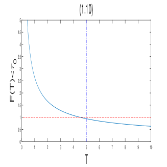
(a)

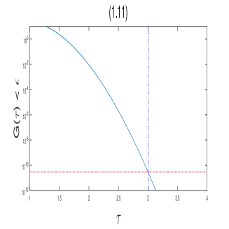
(b)

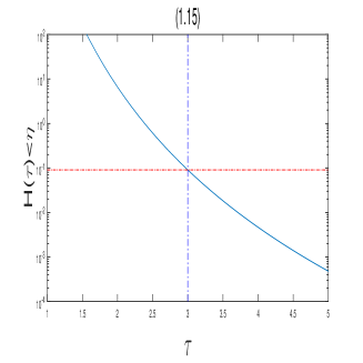
(c)

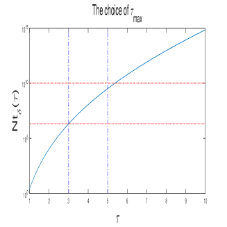
(d)

Figure 1: Computing the trusted frequency region $[\tau_{0},\tau_{max}]$ for $f(t)=t^{2}$: (a) $F(T)$ (b) $G(\tau)$ (c) $H(\tau)$ (d) $N_{t}^{\delta}(\tau)$.

4.2 Trusted frequency region for $f(t)=t^{r},r=0,1,2$ : Numerical computation

The plots presented In Figure 1 enabled us to theoretically investigate the trusted frequency region with error bound 0.017. In this subsection, we numerically investigate the trusted frequency region with an error less than 0.01, (0.1 when $f(t)=1,t$), in Sections 4.2 and 4.3. $T=5$ is fixed as in the previous section. The frequency is specified in increments 0.5 starting from 1, i.e. $1,1.5,2,\cdots$.

At first, in Figure 2(a), we fixed $a=1,N=10^{3},f(t)=t^{2}$ and computed the trusted frequency region with an error bound of 0.01 depending on $N_{t}=10^{3},10^{4},10^{5},10^{6}$. The regions are as follows:

• $N_{t}=10^{3}:\;\;[2.0,5.0]$

• $N_{t}=10^{4}:\;\;[2.0,8.0]$

• $N_{t}=10^{5}:\;\;[2.0,11.0]$

• $N_{t}=10^{6}:\;\;[2.0,15.0]$

This trusted frequency region is larger than the trusted frequency region that was theoretically determined in Section 4.1, even though $N_{t}$ is less than $10^{1}0$ and the error bound is less than $0.017$. The trusted frequency region for the same error bound becomes larger as $N_{t}$ increases.

Next, in Figure 2(b), we fixed $a=1,N=10^{3},N_{t}=10^{3}$ and computed the trusted frequency region with an error bound of 0.1 depending on $f(t)=1,t,t^{2}$. The regions are as follows:

• $f(t)=t^{2}:\;\;[1.0,6.0]$

• $f(t)=t:\;\;[1.0,2.0]$

• $f(t)=1:\;\;$ None

Here, the trusted frequency region becomes larger as $r$ increases. Note that $f(t)=t^{2}$ satisfies the assumption $f(0)=0,f^{\prime}(0)=0$ in Theorem 1.2, whereas $f(t)=1$ and $f(t)=t$ does not.

In Figure 2(c), we fixed $N=10^{3},N_{t}=10^{4},f(t)=t^{2}$ and computed the trusted frequency region with an error bound of 0.01 depending on $a=1,2,3,4$. The regions are as follows:

• $a=1:\;\;[2.0,8.0]$

• $a=2:\;\;[2.0,4.5]$

• $a=3:\;\;[2.5,3.5]$

• $a=4:\;\;[2.5,2.5]$

In this way, we established that the trusted frequency region becomes smaller as $a$ increases.

(a)

(b)

(c)

Figure 2: The approximation $a_{N_{t}}$ of true value $a$ with respect to $\tau$ depending on (a) the number of divisions for the time interval $N_{t}=10^{3},10^{4},10^{5},10^{6}$ when $a=1,N=10^{3},f(t)=t^{2}$ are fixed, (b) the right side function $f(t)=1,t,t^{2}$, when $a=1,N=10^{3},N_{t}=10^{3}$ are fixed, and (c) the true value $a=1,2,3,4$, when $N=10^{3},N_{t}=10^{4},f(t)=t^{2}$ are fixed.

4.3 Trusted frequency region for $f(t)=t^{2}e^{-2t}$ : Numerical computation

We also fixed $a=1,T=5,$ and $N=10^{2}$ in this subsection. We use (2.16) with $\nu=2$ for $u_{N}$, instead of (2.17) which is used when $f(t)=t^{r}$. Figure 3 (a) shows a plot of $e^{2}f(t)$, in which $f(t)$ is normalised for the maximum value to be 1.

In Figure 3(b), we fixed $a=1,N=10^{3},f(t)=t^{2}e^{2-25}$ and computed the trusted frequency region with an error bound of 0.01 depending on $N_{t}=10^{3},10^{4},10^{5},10^{6}$. The regions are as follows:

• $N_{t}=10^{3}:\;\;[2.0,5.0]$

• $N_{t}=10^{4}:\;\;[2.0,8.0]$

• $N_{t}=10^{5}:\;\;[2.0,9.0]$

• $N_{t}=10^{6}:\;\;[2.0,9.0]$

The trusted frequency region becomes larger as $N_{t}$ increases as in the case $f(t)=t^{2}$ in Figure 2(a); however. the region is slightly smaller than that of $f(t)=t^{2}$, especially for $N_{t}=10^{5},10^{6}$. Moreover, the result for $N_{t}=10^{6}$ is slightly better than that of $N_{t}=10^{5}$, although this was not discernable in the figure. The fact that the result for $f(t)=t^{2}$ is better than that for $f(t)=t^{2}e^{-2t}$ comes from the approximation $u_{N}$ in (2.17), where the use of the Reimann-Zeta function improves the result compard to (2.16), where this function was not used. This inference can be verified by the order of convergence $O(N^{-3})$ for $f(t)=t^{2}e^{-2t}$ and $O(N^{-5})$ (with hyperconvergence $O(2^{-N}N^{-3})$ for nonsmall $t$ ) for $f(t)=t^{2}$, which is shown in Lemma 2.6 and Lemma 2.7, respectively.

(a)

(b)

Figure 3: (a) Neumann data $f(t)=t^{2}e^{2-2t}$ at $x=0$ and (b) the approximation of $a=1$, when $f(t)=t^{2}e^{2-2t},N=10^{3},N_{t}=10^{3},10^{4},10^{5},10^{6}$

   

Acknowledgements

This work was partially supported by Grant-in-Aid for Scientific Research (C)(No. 25400155) of Japan Society for the Promotion of Science. KK was also supported by the National Research Foundation of Korea (NRF) funded by the Ministry of Education (NRF-2013R1A1A2010624).