Non-interacting single-impurity Anderson model:
solution without using the equation-of-motion method

Abstract

2015201510.1002andp.20150025952711-12112015794805abstract Ground-state properties of the non-interacting symmetric single-impurity Anderson model (SIAM) are derived from the corresponding eigenenergy equation. Explicit formulae are given for the ground-state energy, the hybridization, and the momentum distribution that are essential quantities for variational approaches to the interacting model. Various spectral functions, e.g., the total density of states, the phase shift function, and the impurity spectral function, are shown to agree with those obtained from the equation-of-motion method (see supplementary material). For a constant hybridization strength and a semi-elliptic host density of states it is seen that the impurity spectral function builds up weight at the band edges.

1 Introduction

The single-impurity Anderson model [1] is one of the fundamental many-body problems in condensed-matter theory. Even its non-interacting limit poses a non-trivial single-particle problem because the electrons on a single site hybridize with those from a conduction band with a large (or infinite) number of degrees of freedom.

The non-interacting single-impurity Anderson model can be solved exactly [1, 2]. Usually, we are interested in the ground-state energy, the density of states, and single-particle Green functions at zero temperature. In textbooks [2, 3], these single-particle properties are calculated from the equation-of-motion approach for the single-particle Green functions. In this communication, we derive them directly from the exact eigenstates and eigenenergies. Apart from being instructive for beginners in many-body theory, the direct approach facilitates a comparison with numerical approaches and covers all general cases (finite bandwidth of the conduction band, bound and anti-bound states). Moreover, ground-state expectation values are important for variational approaches such as the Gutzwiller wave function, see, e.g., [4, 5], so that it is important to have general expressions available for the hybridization and momentum distribution functions. To simplify the discussion, we focus on the symmetric single-impurity Anderson model.

Our work is organized as follows. In chapter 2, we introduce the model Hamiltonian. In chapter 3 we discuss the single-particle Green functions and some of their properties. In chapter 4, we solve the Schrödinger equation where we treat bound/anti-bound states and scattering states separately; we shall take the thermodynamic limit where appropriate. In chapter 5 we derive a variety of ground-state quantities, namely the total energy, the impurity occupancy, the hybridization energy, and the momentum distribution. In chapter 6 we consider the single-particle spectral properties and derive the density of states, the phase shift function, and the impurity spectral function. For comparison, in the supplementary material we re-derive all expressions from the standard equation-of-motion approach. Short conclusions, chapter 7, close our presentation.

2 Model and physical quantities

The Hamiltonian of the single-impurity Anderson model consists of three parts, the host kinetic energy $\hat{T}$, the impurity level $\hat{I}$, and the hybridization $\hat{V}$,

$$\hat{H}=\hat{H}_{0}+\hat{I}\quad,\quad\hat{H}_{0}=\hat{T}+\hat{V}\;.$$ (1)

The eigenstates of the model are denoted by $|\psi_{n}\rangle$. Their energy is $E_{n}$,

$$\hat{H}|\psi_{n}\rangle=E_{n}|\psi_{n}\rangle\;,$$ (2)

and $|\psi_{0}\rangle$ is the ground state with energy $E_{0}$.

2.1 Host electrons

We consider a host system of non-interacting electrons that is described by the host density of states $\rho_{0}(\epsilon)$ in the thermodynamic limit. Since the thermodynamic limit can be delicate for a single impurity in a bath, we discretize the bath levels and describe the host electrons by their kinetic energy

$$\hat{T}=\sum_{k,\sigma}\epsilon(k)\hat{c}_{k,\sigma}^{+}\hat{c}_{k,\sigma}^{\vphantom{+}}\;,$$ (3)

where $\hat{c}_{k,\sigma}^{+}$ ($\hat{c}_{k,\sigma}^{\vphantom{+}}$) creates (annihilates) a spin-$\sigma$ electron in the quantum state $k$ ($\sigma=\uparrow,\downarrow$). For a finite system with $L$ states we have $k=0,1,2,\ldots,(L-1)$, and we choose $L$ to be an odd number for convenience. The thermodynamic limit corresponds to $L\to\infty$.

The band energies are given by the dispersion relation

$$\epsilon(k)=f(-W/2+kW/(L-1))\;,$$ (4)

where $f(-\varepsilon)=-f(\varepsilon)$ is an odd, differentiable and monotonously increasing function that defines the symmetric host density of states $\rho_{0}(\epsilon)=\rho_{0}(-\epsilon)$,

$$\rho_{0}(\epsilon)=\frac{1}{f^{\prime}\left(f^{-1}(\epsilon)\right)}\;.$$ (5)

Later, we shall work with dispersion relations that satisfy

$$f(\pm W/2)=\pm W/2$$ (6)

so that $W>0$ defines the host electron bandwidth. In the following we shall use $W\equiv 1$ as our energy unit. Note that $f(0)=0$, i.e., there is a host state at $k=(L-1)/2$ with zero kinetic energy, $\epsilon((L-1)/2)=0$, and that the completely filled host band has total energy zero, $\sum_{k}\epsilon(k)=0$ because $\epsilon(L-1-k)=-\epsilon(k)$.

Later, we shall give explicit results for a semi-elliptic density of states,

$$\rho_{0}^{\rm se}(\epsilon)=\frac{4}{\pi}\sqrt{1-\left(2\epsilon\right)^{2}\,}\quad,\quad|\epsilon|\leq 1/2$$ (7)

with

$$\int_{-1/2}^{1/2}{\rm d}\epsilon\rho_{0}^{\rm se}(\epsilon)=1\;.$$ (8)

The function $f_{\rm se}(\varepsilon)$ that leads to the semi-elliptic density of states (7) solves the implicit equation

$$\pi\varepsilon=2f_{\rm se}(\varepsilon)\sqrt{1-4[f_{\rm se}(\varepsilon)]^{2}}+\sin^{-1}[2f_{\rm se}(\varepsilon)]\;,$$ (9)

where $\sin^{-1}(z)={\rm arcsin}(z)$ is the inverse sine function. In some cases we shall also give the result for a constant density of states, $f_{\rm cons}(\varepsilon)=\varepsilon$, $\rho_{0}^{\rm cons}(\epsilon)=1$ for $|\epsilon|\leq 1/2$. Note, however, that the constant density of states has some pathological features, e.g., a jump discontinuity at the band edges.

2.2 Impurity level

The impurity level is described by the Hamiltonian

$$\hat{I}=E_{\rm d}\sum_{\sigma}\hat{d}_{\sigma}^{+}\hat{d}_{\sigma}^{\vphantom{+}}+U\hat{d}_{\uparrow}^{+}\hat{d}_{\uparrow}^{\vphantom{+}}\hat{d}_{\downarrow}^{+}\hat{d}_{\downarrow}^{\vphantom{+}}\;.$$ (10)

Here, $E_{\rm d}$ is the energy of the impurity level, and $U$ is the $d$-electrons’ Hubbard interaction. For the symmetric single-impurity Anderson model, we place the impurity level at the particle-hole symmetric energy

$$E_{\rm d}=-U/2\;.$$ (11)

Later we only address the non-interacting case, $U=0$.

2.3 Hybridization

The host electrons and the impurity level can hybridize via

$$\hat{V}=\sqrt{\frac{1}{L}}\sum_{k,\sigma}\left(V_{k,\sigma}\hat{d}_{\sigma}^{+}\hat{c}_{k,\sigma}^{\vphantom{+}}+V_{k,\sigma}^{*}\hat{c}_{k,\sigma}^{+}\hat{d}_{\sigma}^{\vphantom{+}}\right)\;,$$ (12)

where the amplitude $V_{k,\sigma}$ parameterizes the hybridization strength. We demand that the hybridization is independent of spin, $V_{k,\sigma}\equiv V_{k}$. Since $\epsilon(k)$ is a monotonous function of $k$, we may equally write

$$V_{k}\equiv V(\epsilon(k))\;.$$ (13)

Furthermore, we demand that $V_{k}$ is symmetric, $V_{k}=V_{L-1-k}^{*}$, in order to ensure particle-hole symmetry.

2.4 Particle-hole symmetry

We study the case of half band-filling where the total number of electrons $N=N_{\uparrow}+N_{\downarrow}$ equals the total number of levels in the system, $N=L+1$. For the paramagnetic case of interest, we then have $N_{\uparrow}=N_{\downarrow}=N/2=(L+1)/2$.

The particle-hole transformation is defined by

$$\widetilde{\tau}: \hat{c}_{k,\sigma}^{\vphantom{+}}\mapsto\hat{c}_{L-1-k,\sigma}^{+}\quad,\quad\hat{c}_{k,\sigma}^{+}\mapsto\hat{c}_{L-1-k,\sigma}^{\vphantom{+}}\;,$$ (14)

$$\hat{d}_{\sigma}^{\vphantom{+}}\mapsto-\hat{d}_{\sigma}^{+}\quad,\quad\hat{d}_{\sigma}^{+}\mapsto-\hat{d}_{\sigma}^{\vphantom{+}}\;.$$

The transformation leaves the Hamiltonian invariant, i.e., $\hat{H}\mapsto\hat{H}$, because we have $\epsilon(L-1-k)=-\epsilon(k)$ and $V_{k}=V_{L-1-k}^{*}$. Consequently, the same applies to the ground state, $|\psi_{0}\rangle\stackrel{{\scriptstyle\tilde{\tau}}}{{\mapsto}}|\psi_{0}\rangle$. Therefore, we can derive the following relations at half band-filling for the ground-state expectation values

$$n_{k,\sigma} = \langle\hat{c}_{k,\sigma}^{+}\hat{c}_{k,\sigma}^{\vphantom{+}}\rangle=1-n_{L-1-k,\sigma}\;,$$ (15)

$$\langle\hat{d}_{\sigma}^{+}\hat{c}_{k,\sigma}^{\vphantom{+}}\rangle = \langle\hat{c}_{L-1-k,\sigma}^{+}\hat{d}_{\sigma}^{\vphantom{+}}\rangle\;,$$ (16)

$$n_{{\rm d},\sigma} = \langle\hat{d}_{\sigma}^{+}\hat{d}_{\sigma}^{\vphantom{+}}\rangle=1-n_{{\rm d},\sigma}=\frac{1}{2}\;,$$ (17)

where

$$\langle\hat{A}\rangle=\frac{\langle\psi_{0}|\hat{A}|\psi_{0}\rangle}{\langle\psi_{0}|\psi_{0}\rangle}\;.$$ (18)

Equation (17) proves that the $d$-level is half filled for any dispersion relation and hybridization, $n_{{\rm d},\sigma}=1/2$. Note that the relations (15)–(17) apply to the interacting case, $U\geq 0$.

3 Single-particle Green functions

3.1 Retarded, advanced, and causal Green functions

For Heisenberg operators ($\hbar\equiv 1$)

$$\hat{A}(t)=e^{{\rm i}\hat{H}t}\hat{A}e^{-{\rm i}\hat{H}t}$$ (19)

we consider the causal Green function

$$G_{A,B}^{\rm c}(t)=(-{\rm i})\langle{\cal T}\left(\hat{A}(t)\hat{B}\right)\rangle\;,$$ (20)

where ${\cal T}$ is the time-ordering operator,

$${\cal T}\left(\hat{A}(t)\hat{B}\right)=\left\{\begin{array}[]{@{}lcl@{}}\hphantom{-}\hat{A}(t)\hat{B}&\hbox{for}&t>0\\ -\hat{B}\hat{A}(t)&\hbox{for}&t<0\end{array}\right.\;.$$ (21)

The sign applies for Fermion operators $\hat{A},\hat{B}$. The retarded and advanced Green functions are defined by

$$G_{A,B}^{\rm ret}(t) = (-{\rm i})\Theta(t)\langle\left[\hat{A}(t),\hat{B}\right]_{+}\rangle\;,$$

$$G_{A,B}^{\rm adv}(t) = {\rm i}\Theta(-t)\langle\left[\hat{A}(t),\hat{B}\right]_{+}\rangle\;,$$ (22)

where $\Theta(t)$ is the Heaviside step-function.

3.2 Fourier transformation

For later use we introduce the Fourier transformation (FT)

$$f(t) = \int_{-\infty}^{\infty}\frac{{\rm d}\omega}{2\pi}e^{-\eta|\omega|}e^{-{\rm i}\omega t}\tilde{f}(\omega)\;,$$

$$\tilde{f}(\omega) = \int_{-\infty}^{\infty}{\rm d}te^{-\eta|t|}e^{{\rm i}\omega t}f(t)\;,$$ (23)

where the factors $\exp(-\eta|\omega|)$ and $\exp(-\eta|t|)$ with $\eta=0^{+}$ ensure the convergence of the integrals. They shall be set to zero whenever the convergence of integrals or other expressions is guaranteed at $\eta=0$.

We use a complete set of eigenstates for the Hamiltonian $\hat{H}$, see equation (2), to derive the Lehmann representation of the causal and retarded Green functions,

$$\tilde{G}_{A,B}^{\rm c}(\omega) = \sum_{n}\biggl{[}\frac{\langle\psi_{0}|\hat{A}|\psi_{n}\rangle\langle\psi_{n}|\hat{B}|\psi_{0}\rangle}{E_{0}-E_{n}+\omega+{\rm i}\eta}$$ (24)

$$\hphantom{\sum_{n}\biggl{[}}+\frac{\langle\psi_{0}|\hat{B}|\psi_{n}\rangle\langle\psi_{n}|\hat{A}|\psi_{0}\rangle}{E_{n}-E_{0}+\omega-{\rm i}\eta}\biggr{]}\;,$$

$$\tilde{G}_{A,B}^{\rm ret}(\omega) = \sum_{n}\biggl{[}\frac{\langle\psi_{0}|\hat{A}|\psi_{n}\rangle\langle\psi_{n}|\hat{B}|\psi_{0}\rangle}{E_{0}-E_{n}+\omega+{\rm i}\eta}$$ (25)

$$\hphantom{\sum_{n}\biggl{[}}+\frac{\langle\psi_{0}|\hat{B}|\psi_{n}\rangle\langle\psi_{n}|\hat{A}|\psi_{0}\rangle}{E_{n}-E_{0}+\omega+{\rm i}\eta}\biggr{]}\;.$$

The Lehmann representation shows that the real parts of the causal and retarded Green function agree and that their imaginary parts differ in sign for $\omega<0$. Therefore, we can derive the causal Green function from the retarded Green function by the simple substitution

$$\tilde{G}_{A,B}^{\rm c}(\omega)=\left.\tilde{G}_{A,B}^{\rm ret}(\omega)\right|_{\omega+{\rm i}\eta\to\omega+{\rm i}{\rm sgn}(\omega)\eta}$$ (26)

in frequency space where ${\rm sgn}(u)=\Theta(u)-\Theta(-u)$ is the sign function.

3.3 Spectral function and density of states

Finally, we define the spectral function for the Fermion Green function as

$$D_{A,B}(\omega)=-\frac{1}{\pi}{\rm Im}\left(\tilde{G}_{A,B}^{\rm ret}(\omega)\right)\;.$$ (27)

The Lehmann representation shows that it is positive semi-definite if $\hat{A}=\hat{B}^{+}$.

When we use the operators for single-particle eigenstates of $\hat{H}_{0}$ with eigenenergies $E(m)$, $\hat{A}=\hat{a}_{m,\sigma}^{\vphantom{+}}$ and $\hat{B}=\hat{a}_{m,\sigma}^{+}$, see chapter 4, we find from the Lehmann representation

$$D_{\sigma}(\omega)=\frac{1}{L}\sum_{m}D_{m,\sigma;m,\sigma}(\omega)=\frac{1}{L}\sum_{m}\delta(\omega-E(m))$$ (28)

because we have $E_{m}=E(m)+E_{0}$ ($E_{m}=-E(m)+E_{0}$) for a single-particle (single-hole) excitation of the ground state for non-interacting particles. Apparently, $D_{\sigma}(\omega)$ describes the density of states for single-particle excitations with spin $\sigma$.

4 Solution of the Schrödinger equation

We analyze the non-interacting Hamiltonian $\hat{H}_{0}=\hat{T}+\hat{V}$ for large but finite system sizes $L$. We shall take the thermodynamic limit, $L\to\infty$, where appropriate.

4.1 Derivation of the eigenvalue equation

Since $\hat{H}_{0}$ poses a single-particle problem, we may write

$$\hat{H}_{0}=\sum_{m=0,\sigma}^{L}E(m)\hat{a}_{m,\sigma}^{+}\hat{a}_{m,\sigma}^{\vphantom{+}}\;,$$ (29)

where

$$\hat{a}_{m,\sigma}^{+}=g_{m}^{*}\hat{d}_{\sigma}^{+}+\sqrt{\frac{1}{L}}\sum_{n=0}^{L-1}\lambda_{m}^{*}(n)\hat{c}_{n,\sigma}^{+}$$ (30)

is the Fermion creation operator for an exact eigenmode with energy $E(m)$. The $L+1$ energies are labeled in ascending order, $E(m-1)<E(m)$, $m=1,2,\ldots,L$.

The orthonormality condition

$$\left[\hat{a}_{m,\sigma}^{+},\hat{a}_{m^{\prime},\sigma^{\prime}}^{\vphantom{+}}\right]_{+}=\delta_{\sigma,\sigma^{\prime}}\delta_{m,m^{\prime}}$$ (31)

implies

$$1=|g_{m}|^{2}+\frac{1}{L}\sum_{n=0}^{L-1}|\lambda_{m}(n)|^{2}\;.$$ (32)

Equation (29) can only hold if

$$\left[\hat{H}_{0},\hat{a}_{m,\sigma}^{+}\right]_{-}=E(m)\hat{a}_{m,\sigma}^{+}\;.$$ (33)

To express this equation in terms of the original operators, see equation (30), we use

$$\left[\hat{T},\hat{a}_{m,\sigma}^{+}\right]_{-} = \sqrt{\frac{1}{L}}\sum_{n=0}^{L-1}\lambda_{m}^{*}(n)\epsilon(n)\hat{c}_{n,\sigma}^{+}\;,$$ (34)

$$\left[\hat{V},\hat{a}_{m,\sigma}^{+}\right]_{-} = \sqrt{\frac{1}{L}}g_{m}^{*}\sum_{n=0}^{L-1}V_{n}\hat{c}_{n,\sigma}^{+}+\left(\frac{1}{L}\sum_{n=0}^{L-1}V_{n}\lambda_{m}^{*}(n)\right)\hat{d}_{\sigma}^{+}\;.$$

A comparison with equation (33) leads to the conditions

$$E(m)g_{m}^{*} = \frac{1}{L}\sum_{n=0}^{L-1}V_{n}\lambda_{m}^{*}(n)\;,$$ (36)

$$E(m)\lambda_{m}^{*}(n) = \epsilon(n)\lambda_{m}^{*}(n)+g_{m}^{*}V_{n}^{*}\;.$$ (37)

We thus find

$$\lambda_{m}(n)=g_{m}\frac{V_{n}}{E(m)-\epsilon(n)}$$ (38)

with the energies from the eigenenergy equation [1, 3]

$$E(m)=\frac{1}{L}\sum_{n=0}^{L-1}\frac{|V_{n}|^{2}}{E(m)-\epsilon(n)}\;.$$ (39)

The solutions of the eigenenergy equation provide all the information about the finite-size system. The normalization condition (32) reduces to

$$|g_{m}|^{2}=|g(E(m))|^{2}=\left(1+\frac{1}{L}\sum_{n=0}^{L-1}\frac{|V_{n}|^{2}}{(E(m)-\epsilon(n))^{2}}\right)^{-1}\;.$$ (40)

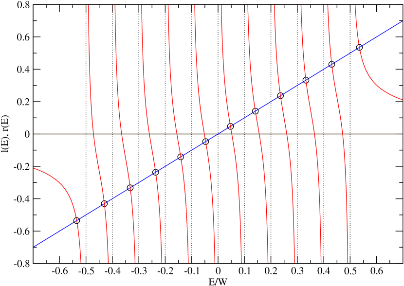
Figure 1: Graphical solution of the eigenenergy equation (39) for $L=11$, $V_{n}^{2}/L=0.01$, and a linear dispersion relation, $\epsilon(n)=-1/2+n/(L-1)$. The left-hand-side of equation (39), $l(E)=E$, is shown as a straight, blue line, the right-hand-side of equation (39), $r(E)=\sum_{n=0}^{L-1}(V_{n}^{2}/L)/[E-\epsilon(n)]$, is shown by the red lines. Their intersections, $l(E(m))=r(E(m))$, the eigenenergies, are encircled. For $E<-1/2$ ($E>1/2$) we find the (anti-)bound states, the scattering states lie in the interval $|E|<1/2$. The vertical dotted lines indicate the divergences of $r(E)$ at $E=\epsilon(n)$, $n=0,\ldots,L-1$.

As an example, in figure 1 we show the graphical solution of the eigenenergy equation (39) for $L=11$ and $V_{n}^{2}/L=0.01$ and a linear dispersion relation, $\epsilon(k)=-1/2+k/(L-1)$ (bandwidth $W=1$). The figure displays particle-hole symmetry, and bound/anti-bound states as well as scattering states, as we discuss in the remainder of this section.

4.2 Particle-hole symmetry

If $E(m)$ is a solution of the eigenenergy equation (39), $[-E(m)]$ also is a solution. This is easily shown with the help of particle-hole symmetry,

$$\frac{1}{L}\sum_{n=0}^{L-1}\frac{|V_{n}|^{2}}{-E(m)-\epsilon(n)} = -\frac{1}{L}\sum_{n=0}^{L-1}\frac{|V_{n}|^{2}}{E(m)+\epsilon(n)}$$ (41)

$$= -\frac{1}{L}\sum_{n=0}^{L-1}\frac{|V_{L-1-n}|^{2}}{E(m)+\epsilon(L-1-n)}$$

$$= -\frac{1}{L}\sum_{n=0}^{L-1}\frac{|V_{n}|^{2}}{E(m)-\epsilon(n)}=-E(m)\;,$$

where we used the symmetry conditions $V_{n}=V_{L-1-n}^{*}$ and $\epsilon(n)=-\epsilon(L-1-n)$. Therefore, using our energy labeling, we find $E(L-m)=-E(m)$ for $m=0,1,\ldots,L$.

4.3 Bound/anti-bound states

Outside the band edges, bound and anti-bound states can form. In the thermodynamic limit, their energies $E_{\rm b}<-1/2$ ($E_{\rm ab}>1/2$) are obtained from the solution of the integral equation

$$E_{\rm b/ab}=\int_{-1/2}^{1/2}{\rm d}\epsilon\rho_{0}(\epsilon)\frac{|V(\epsilon)|^{2}}{E_{\rm b/ab}-\epsilon}\;.$$ (42)

Their existence depends on the shape of the host density of states $\rho_{0}(\epsilon)$ and of the hybridization $V(\epsilon)$. If the density of states continuously goes to zero at the band edges and the hybridization is well-behaved, there are no bound/anti-bound states in the limit of small hybridization, $|V(\epsilon)|^{2}\ll 1$.

For example, when we use the semi-elliptic density of states (7) and a constant hybridization in equation (42) we find the condition

$$\frac{1}{4V^{2}}=2-\sqrt{4-\frac{1}{(E_{\rm b/ab}^{\rm se})^{2}}}\;.$$ (43)

For $V<1/4$, the semi-elliptic density of states does not support bound/anti-bound states. For $V>1/4$, the bound/anti-bound levels lie at $E_{\rm b/ab}^{\rm se}=\pm 4V^{2}/\sqrt{16V^{2}-1}$. In contrast, for a constant density of states and a constant hybridization, equation (42) leads to

$$E_{\rm a/ab}^{\rm cons}=V^{2}\ln\left|\frac{1+2E_{\rm a/ab}^{\rm cons}}{1-2E_{\rm a/ab}^{\rm cons}}\right|\;.$$ (44)

For small $V<1/4$, the bound/anti-bound levels lie at $E_{\rm b/ab}^{\rm cons}\approx\pm(1/2+\exp[-1/(2V^{2})])$. The (anti-)binding energy is exponentially small but finite for small $V$.

The existence of (anti-)bound states influences the energy levels in the vicinity of the band edges. Although these effects often are negligibly small, in the following we restrict ourselves to situations where bound/anti-bound states are absent as for the semi-elliptic density of states for a constant, small hybridization $V<1/4$.

4.4 Scattering states

For all other states, the impurity scattering induces energy shifts of the order of $1/L$. Therefore, in equation (39) we set

$$E(m)=\epsilon(m)+\frac{x(\epsilon(m))}{L}\quad,\quad|x(\epsilon(m))|={\cal O}\left(1\right)\;,$$ (45)

where $x(\epsilon(m))$ quantifies the scattering energy shift introduced by the impurity. Note that $x(\epsilon)<0$ ($x(\epsilon)>0$) for $\epsilon<0$ ($\epsilon>0$) because the impurity level at energy $\epsilon=0$ repels the host energy levels. We shall show that $x(0^{+})=1/(2\rho_{0}(0))$ so that $x(\epsilon)$ is discontinuous at $\epsilon=0$.

In order to solve the eigenvalue equation (39) for large systems we start with the observation that the Taylor expansion for finite $r\ll L$ leads to the following approximation

$$L(\epsilon(m+r)-\epsilon(m))\approx rf^{\prime}\left(f^{-1}(\epsilon(m))\right)=\frac{r}{\rho_{0}(\epsilon(m))}\;,$$ (46)

with corrections of the order $1/L$, see equations (4), (5). In the limit of large system size and not infinitesimally close to the band edges, we can write

$$\sum_{n=0}^{L-1}\frac{|V(\epsilon(n))|^{2}/L}{E(m)-\epsilon(n)} = \lim_{R\to\infty}\sum_{r=-R}^{R}\!\frac{|V(\epsilon(m+r))|^{2}}{x(\epsilon(m))-L(\epsilon(m+r)-\epsilon(m))}$$ (47)

$$+\Lambda_{V}(E(m))\;,$$

where

$$\Lambda_{V}(E)={\cal P}\int_{-1/2}^{1/2}{\rm d}\epsilon\rho_{0}(\epsilon)\frac{|V(\epsilon)|^{2}}{E-\epsilon}\;,$$ (48)

and ${\cal P}$ denotes the Cauchy principal value integral. For constant hybridization and the semi-elliptic density of states we have for $|E|<1/2$

$$\Lambda_{V}^{\rm se}(E)=8V^{2}E\;.$$ (49)

This particularly simple form permits explicit calculations, see below.

For the derivation of equation (47) we singled out the region $|m-n|\leq R$ ($1\ll R\ll L$) from the sum over $n$ before we employed the Euler-Maclaurin sum formula,

$$\sum_{n=N_{a}}^{N_{b}}h(n)=\int_{N_{a}}^{N_{b}}{\rm d}nh(n)+\frac{1}{2}\left(h(N_{a})+h(N_{b})\right)+\ldots$$ (50)

that generates the contribution $\Lambda_{V}(E)$ in equation (47). For the first term in equation (47) we use equation (46)

$$\sum_{r=-\infty}^{\infty}\frac{|V(\epsilon(m+r))|^{2}}{x(\epsilon(m))-L(\epsilon(m+r)-\epsilon(m))}\approx|V(\epsilon(m))|^{2}\rho_{0}(\epsilon(m))$$

$$\times\sum_{r=-\infty}^{\infty}\frac{1}{x(\epsilon(m))\rho_{0}(\epsilon(m))-r}\;.$$

Using equation (1.421,3) of Ref. [6] we find

$$\sum_{r=-\infty}^{\infty}\frac{|V(\epsilon(m+r))|^{2}}{x(\epsilon(m))-L(\epsilon(m+r)-\epsilon(m))}\approx\pi\rho_{0}(\epsilon(m))|V(\epsilon(m)|^{2}$$

$$\times\cot\left[\pi\rho_{0}(\epsilon(m))x(\epsilon(m))\right]\;.$$

(52)

Here we used the fact that $V(\epsilon)$ is a smooth function so that $|V(\epsilon(m+r))|^{2}\approx|V(\epsilon(m))|^{2}+{\cal O}(1/L)$. To leading order in $1/L$, the eigenvalue equation (39) leads to

$$x(\epsilon)=\frac{1}{\pi\rho_{0}(\epsilon)}\cot^{-1}\left[\frac{\epsilon-\Lambda_{V}(\epsilon)}{\pi|V(\epsilon)|^{2}\rho_{0}(\epsilon)}\right]\;.$$ (53)

This is the desired equation for the scattering energy shifts; for a constant density of states, the derivation can be found as equation (I-12) in Ref. [7].

For later use, we define

$$x(\epsilon) = \frac{1}{2\rho_{0}(\epsilon)}\left(\Theta(\epsilon)-\Theta(-\epsilon)\right)-y(\epsilon)\;,$$

$$y(\epsilon) = \frac{1}{\pi\rho_{0}(\epsilon)}\tan^{-1}\left[\frac{\epsilon-\Lambda_{V}(\epsilon)}{\pi|V(\epsilon)|^{2}\rho_{0}(\epsilon)}\right]\;.$$ (54)

Note that, for a smooth hybridization $V(\epsilon)$, the function $y(\epsilon)$ is continuous in the interval $|\epsilon|\leq 1/2$.

5 Ground-state expectation values

According to equation (29) the ground state of $\hat{H}_{0}$ is given by

$$|\psi_{0}\rangle=\prod_{\sigma}\prod_{m=0}^{(L-1)/2}\hat{a}_{m,\sigma}^{+}|\hbox{vac}\rangle\;.$$ (55)

5.1 Ground-state energy

We are interested in the change $\Delta E$ of the ground-state energy due to the hybridization of the impurity and the host electrons. In the absence of bound/anti-bound states, it is given by

$$\frac{\Delta E}{2}=\sum_{m=0}^{(L-1)/2}\left[E(m)-\epsilon(m)\right]\;.$$ (56)

Here we took into account that the $(L+1)/2$ states lowest in energy are occupied for each spin species. Moreover, $\epsilon((L-1)/2)=0$ and the impurity level is at $E_{\rm d}=0$ so that they do not contribute in the case of vanishing hybridization.

The Euler-Maclaurin formula (50) and the definition of the host density of states (5) lead to

$$\frac{\Delta E}{2}=\int_{-1/2}^{0}{\rm d}\epsilon\rho_{0}(\epsilon)x(\epsilon)=\int_{-1/2}^{0}\frac{{\rm d}\epsilon}{\pi}\cot^{-1}\left[\frac{\epsilon-\Lambda_{V}(\epsilon)}{\pi|V(\epsilon)|^{2}\rho_{0}(\epsilon)}\right]$$ (57)

in the thermodynamic limit where we inserted the scattering energy shifts from equation (53).

Equation (57) can be evaluated further in the limit of vanishingly small hybridization. We set $V(\epsilon)=Vv(\epsilon)$ with $v(0)=1$ and consider $V\to 0$. Then,

$$\frac{\Delta E}{2}\approx\frac{V^{2}}{\pi}\int_{-1/2}^{-cV^{2}}{\rm d}\epsilon\frac{\pi|v(\epsilon)|^{2}\rho_{0}(\epsilon)}{\epsilon}$$ (58)

with a low-energy cut-off, $c={\cal O}(1)$. To leading order in $V^{2}\ln(1/V^{2})$ we then find

$$\frac{\Delta E}{2}(V\to 0)=-\rho_{0}(0)V^{2}\ln\left(\frac{1}{V^{2}}\right)+{\cal O}\left(V^{2}\right)\;.$$ (59)

For a constant hybridization and the semi-elliptic density of states we find for all $|V|<1/4$

$$\frac{(\Delta E)^{\rm se}(V)}{2}=-\frac{\alpha}{2\pi}\frac{\tanh^{-1}\left[\sqrt{1-\alpha^{2}}\right]}{\sqrt{1-\alpha^{2}}}\quad,\quad\alpha=\frac{8V^{2}}{1-8V^{2}}\;.$$ (60)

For small $V$ this can be approximated as ($\ln(e)=1$)

$$\frac{(\Delta E)^{\rm se}(V)}{2} = -\frac{4}{\pi}V^{2}\left[\ln\left(\frac{1}{4V^{2}}\right)+8V^{2}\ln\left(\frac{1}{4eV^{2}}\right)\right]$$

$$+{\cal O}\left(V^{6}\ln(V^{2})\right)$$

$$= -\frac{\Gamma}{\pi}\left[\ln\left(\frac{1}{\Gamma}\right)+8V^{2}\ln\left(\frac{1}{e\Gamma}\right)\right]+{\cal O}\left(V^{6}\ln(V^{2})\right)\;,$$

$$\Gamma = \pi\rho_{0}(0)V^{2}\;.$$ (61)

For a constant hybridization and a constant density of states, the small-$V$ expansion of the ground-state energy shift is given by

$$\frac{(\Delta E)^{\rm cons}(V)}{2} = -V^{2}\left[\ln\left(\frac{e}{2\pi V^{2}}\right)+4V^{2}\ln\left(\frac{1}{V^{2}}\right)\right]+{\cal O}\left(V^{4}\right)$$

$$= -\frac{\Gamma}{\pi}\left[\ln\left(\frac{e}{2\Gamma}\right)+4V^{2}\ln\left(\frac{\pi}{\Gamma}\right)\right]+{\cal O}\left(V^{4}\right)\;.$$

The comparison with the general low-$V$ expansion (59) shows that the correction of the order ${\cal O}(V^{2})$ depends on the shape of the host density of states.

5.2 Impurity occupancy

With the help of

$$\left[\hat{d}_{\sigma}^{+}\hat{d}_{\sigma}^{\vphantom{+}},\hat{a}_{m,\sigma^{\prime}}^{+}\right]_{-}=\delta_{\sigma,\sigma^{\prime}}g_{m}^{*}\hat{d}_{\sigma}^{+}$$ (62)

we find that

$$\langle\hat{d}_{\sigma}^{+}\hat{d}_{\sigma}^{\vphantom{+}}\rangle=\sum_{m=0}^{(L-1)/2}|g_{m}|^{2}\;.$$ (63)

Equation (40) shows that $|g_{L-m}|^{2}=|g_{m}|^{2}$ so that

$$\sum_{m=0}^{L}|g_{m}|^{2}=2\sum_{m=0}^{(L-1)/2}|g_{m}|^{2}=2\langle\hat{d}_{\sigma}^{+}\hat{d}_{\sigma}^{\vphantom{+}}\rangle\;.$$ (64)

The expression on the left-hand side corresponds to the probability to find the $d$-level occupied in a completely filled system,

$$\sum_{m=0}^{L}|g_{m}|^{2}=1\;.$$ (65)

Therefore we find the result

$$\langle\hat{d}_{\sigma}^{+}\hat{d}_{\sigma}^{\vphantom{+}}\rangle=\frac{1}{2}$$ (66)

as a consequence of particle-hole symmetry, in agreement with equation (17).

It is instructive to derive equation (66) explicitly. From equation (45) we find up to terms of ${\cal O}(1)$

$$\sum_{n=0}^{L-1}\frac{|V(n)|^{2}/L}{(E(m)-\epsilon(n))^{2}}=-\frac{\partial}{\partial x(\epsilon(m))}\left[\sum_{n=0}^{L-1}\frac{|V(n)|^{2}}{E(m)-\epsilon(n)}\right]\;,$$ (67)

so that from equation (52) we find

$$\sum_{n=0}^{L-1}\frac{|V(n)|^{2}/L}{(E(m)-\epsilon(n))^{2}}=L\frac{[\pi\rho_{0}(\epsilon(m)|V(\epsilon(m))|]^{2}}{\sin^{2}[\pi\rho_{0}(\epsilon(m))x(\epsilon(m))]}\;.$$ (68)

Therefore, equations (40) and (53) give

$$|g_{m}|^{2} = \frac{1}{L}|g(\epsilon(m))|^{2}\;,$$

$$|g(\epsilon)|^{2} = \frac{|V(\epsilon)|^{2}}{[\pi\rho_{0}(\epsilon)|V(\epsilon)|^{2}]^{2}+[\epsilon-\Lambda_{V}(\epsilon)]^{2}}\;,$$ (69)

where we used equation (53) for $x(E)$. Then, from equation (63)

$$\langle\hat{d}_{\sigma}^{+}\hat{d}_{\sigma}^{\vphantom{+}}\rangle = \int_{-1/2}^{0}{\rm d}E\rho_{0}(E)|g(E)|^{2}$$ (70)

$$= \int_{-1/2}^{0}{\rm d}E\frac{\rho_{0}(E)|V(E)|^{2}}{[\pi\rho_{0}(E)|V(E)|^{2}]^{2}+[E-\Lambda_{V}(E)]^{2}}\;.$$

Using $\rho_{0}(-E)=\rho_{0}(E)$, $|V(-E)|^{2}=|V(E)|^{2}$, and $\Lambda_{V}(-E)=-\Lambda_{V}(E)$ due to particle-hole symmetry, we can write

$$2\langle\hat{d}_{\sigma}^{+}\hat{d}_{\sigma}^{\vphantom{+}}\rangle=\int_{-1/2}^{1/2}{\rm d}E\frac{\rho_{0}(E)|V(E)|^{2}}{[\pi\rho_{0}(E)|V(E)|^{2}]^{2}+[E-\Lambda_{V}(E)]^{2}}=1$$ (71)

because the integral in equation (71) gives the result for a completely filled band. Therefore, we find $\langle\hat{d}_{\sigma}^{+}\hat{d}_{\sigma}^{\vphantom{+}}\rangle=1/2$ again.

5.3 Hybridization

With the help of

$$\left[\hat{c}_{k,\sigma}^{+}\hat{d}_{\sigma}^{\vphantom{+}},\hat{a}_{m,\sigma^{\prime}}^{+}\right]_{-}=\delta_{\sigma,\sigma^{\prime}}g_{m}^{*}\hat{c}_{k,\sigma}^{+}$$ (72)

we find that

$$\langle\hat{c}_{k,\sigma}^{+}\hat{d}_{\sigma}^{\vphantom{+}}\rangle = \sqrt{\frac{1}{L}}\sum_{m=0}^{(L-1)/2}g_{m}^{*}\lambda_{m}(k)$$ (73)

$$= \sqrt{\frac{1}{L}}\sum_{m=0}^{(L-1)/2}|g_{m}|^{2}\frac{V_{k}}{E(m)-\epsilon(k)}\;.$$

In the thermodynamic limit, this expression can be transformed into

$$\langle\hat{c}_{k,\sigma}^{+}\hat{d}_{\sigma}^{\vphantom{+}}\rangle \equiv \frac{V_{k}}{\sqrt{L}}\left[G(\epsilon(k))+H(\epsilon(k))\right]\;,$$ (74)

$$G(\epsilon) = \Theta(-\epsilon)|g(\epsilon)|^{2}\frac{\left[\epsilon-\Lambda_{V}(\epsilon)\right]}{|V(\epsilon)|^{2}}$$ (75)

$$= \Theta(-\epsilon)\frac{\epsilon-\Lambda_{V}(\epsilon)}{\left[\pi\rho_{0}(\epsilon)|V(\epsilon)|^{2}\right]^{2}+\left[\epsilon-\Lambda_{V}(\epsilon)\right]^{2}}\;,$$

$$H(\epsilon) = \int_{-1/2}^{0}\frac{{\rm d}E}{E-\epsilon}\frac{\rho_{0}(E)|V(E)|^{2}}{[\pi\rho_{0}(E)|V(E)|^{2}]^{2}+[E-\Lambda_{V}(E)]^{2}}\;,$$

where the integral on the right-hand side of equation (LABEL:eq:Hintegral) must be understood as a principal value integral when $-1/2<\epsilon<0$. The derivation of $G(\epsilon)$ proceeds along the lines developed in Sect. 4.4.

In general, $H(\epsilon)$ cannot be calculated analytically. In the limit of vanishing hybridization, $V(\epsilon)=Vv(\epsilon)$ with $v(0)=1$ and $V\to 0$, we find

$$H(\epsilon,V\to 0) \approx \int_{-\infty}^{0}{\rm d}E\frac{V^{2}\rho_{0}(0)}{[\pi\rho_{0}(0)V^{2}]^{2}+E^{2}}\frac{1}{E-\epsilon}$$ (77)

$$= -\frac{\epsilon}{2[(\pi\rho_{0}(0)V^{2})^{2}+\epsilon^{2}]}$$

$$+\rho_{0}(0)V^{2}\frac{\ln\left(|\epsilon|/(\pi\rho_{0}(0)V^{2})\right)}{(\pi\rho_{0}(0)V^{2})^{2}+\epsilon^{2}}\;.$$

Apparently, the hybridization matrix element is logarithmically divergent near $\epsilon=0$. This does not cause any problems because $\langle\hat{c}_{k,\sigma}^{+}\hat{d}_{\sigma}^{\vphantom{+}}\rangle\sim[G(\epsilon(k))+H(\epsilon(k))]/\sqrt{L}$ remains bounded since the smallest accessible values for $\epsilon(k)$ is of the order of $1/L$. For a constant hybridization and the semi-elliptic density of states, $H^{\rm se}(\epsilon)$ can be calculated analytically. The lengthy expressions agree very well with $H(\epsilon,V\to 0)$ for all $V<0.1$.

The contribution of the hybridization to the ground-state energy per spin is given by

$$\frac{\langle\hat{V}\rangle}{2}=2\int_{-1/2}^{1/2}{\rm d}\epsilon\rho_{0}(\epsilon)|V(\epsilon)|^{2}\left[H(\epsilon)+G(\epsilon)\right]\;.$$ (78)

In the limit of vanishingly small hybridization, $H(\epsilon)$ does not contribute to the hybridization energy. The first term of $H(\epsilon)$ in equation (77) is odd and thus cancels out when integrated over the whole band. The second term apparently is of the order $V^{4}\ln(V^{2})$ and thus smaller by a factor of $V^{2}$ than the leading-order term. Therefore, we have

$$\frac{\langle\hat{V}\rangle}{2}(V\to 0) \approx 2\int_{-cV^{2}}^{0}{\rm d}\epsilon\frac{\rho_{0}(0)V^{2}\epsilon}{\left[\pi\rho_{0}(0)V^{2}\right]^{2}+\epsilon^{2}}$$ (79)

$$= -2\frac{\Gamma}{\pi}\ln\left(\frac{1}{\Gamma}\right)+{\cal O}\left(V^{2}\right)=2\frac{\Delta E}{2}(V\to 0)\;,$$

see equation (61). The energy gain through the hybridization is twice as large as the energy loss due to the distortion of the Fermi sea, as we show next.

5.4 Momentum distribution

With the help of

$$\left[\hat{c}_{k,\sigma}^{+}\hat{c}_{k,\sigma}^{\vphantom{+}},\hat{a}_{m,\sigma^{\prime}}^{+}\right]_{-}=\delta_{\sigma,\sigma^{\prime}}\sqrt{\frac{1}{L}}\lambda_{m}^{*}(k)\hat{c}_{k,\sigma}^{+}$$ (80)

we find that

$$\langle\hat{c}_{k,\sigma}^{+}\hat{c}_{k,\sigma}^{\vphantom{+}}\rangle = \frac{1}{L}\sum_{m=0}^{(L-1)/2}|\lambda_{m}(k)|^{2}$$ (81)

$$= \frac{1}{L}\sum_{m=0}^{(L-1)/2}|g_{m}|^{2}\frac{|V_{k}|^{2}}{(E(m)-\epsilon(k))^{2}}\;.$$

The thermodynamic limit is more subtle than for the hybridization matrix element because terms of order unity appear next to terms of order $1/L$. Proceeding along the lines of Sect. 4.4 we find to leading order

$$\langle\hat{c}_{k,\sigma}^{+}\hat{c}_{k,\sigma}^{\vphantom{+}}\rangle^{(0)}\equiv n^{(0)}(\epsilon(k))=\Theta\left(-\epsilon(k)\right)\;.$$ (82)

The $1/L$ corrections are obtained as

$$L\langle\hat{c}_{k,\sigma}^{+}\hat{c}_{k,\sigma}^{\vphantom{+}}\rangle^{(1)} \equiv n^{(1)}(\epsilon(k))$$ (83)

$$= |V_{k}|^{2}\frac{\partial}{\partial u}\left[\sum_{m=0}^{(L-1)/2}|g_{m}|^{2}\frac{1}{E(m)-u}\right]_{u=\epsilon(k)}$$

$$= |V_{k}|^{2}\left[G^{\prime}(\epsilon(k))+H^{\prime}(\epsilon(k))\right]$$

with $G(\epsilon)$ and $H(\epsilon)$ from equations (75) and (LABEL:eq:Hintegral), respectively. The total momentum distribution is given by $n(\epsilon(k))=n^{(0)}(\epsilon(k))+n^{(1)}(\epsilon(k))/L$.

Our analysis of the function $H(\epsilon)$ in the previous subsection shows that the momentum distribution develops a $1/\epsilon$ singularity for $\epsilon\to 0$ because $H(\epsilon)\sim\ln(|\epsilon|)$ so that $H^{\prime}(\epsilon)\sim 1/\epsilon$ for $\epsilon\to 0$. However, its strength is proportional to $V^{4}/L$ for small $V$ so that, for the smallest accessible value for $\epsilon(k)$, the contribution to the momentum distribution actually remains small.

The contribution of the host electrons to the ground-state energy is given by

$$\frac{\Delta T}{2}=\frac{\langle\hat{T}\rangle-T_{0}}{2} = \int_{-1/2}^{1/2}{\rm d}\epsilon\epsilon\rho_{0}(\epsilon)L\left(n(\epsilon)-\Theta(-\epsilon)\right)$$

$$= \int_{-1/2}^{1/2}{\rm d}\epsilon\epsilon\rho_{0}(\epsilon)|V(\epsilon)|^{2}\left[G^{\prime}(\epsilon)+H^{\prime}(\epsilon)\right]\;,$$

where

$$T_{0}=2L\int_{-1/2}^{0}{\rm d}\epsilon\epsilon\rho_{0}(\epsilon)$$ (85)

is the energy of the undisturbed host band. As for the hybridization energy, the function $G(\epsilon)$ gives the dominant contribution in the limit of small hybridizations. We find after a partial integration

$$\frac{\Delta T}{2}(V\to 0) \approx V^{2}\rho_{0}(0)\int_{-cV^{2}}^{0}{\rm d}\epsilon G(\epsilon)$$ (86)

$$= V^{2}\rho_{0}(0)\int_{-cV^{2}}^{0}{\rm d}\epsilon\frac{\epsilon}{(\pi\rho_{0}(0)V^{2})^{2}+\epsilon^{2}}$$

$$= \frac{\Gamma}{\pi}\ln\left(\frac{1}{\Gamma}\right)=-\frac{E_{0}}{2}(V\to 0)\;,$$

including only the leading-order terms, of the order of ${\cal O}\left(V^{2}\ln(1/V^{2})\right)$. Equation (86) shows that, indeed, the host electrons’ loss in energy is half of the gain due to their hybridization with the impurity, compare equation (79).

6 Spectral properties

In this chapter we derive the single-particle spectral properties. In the supplementary material, we use the equation-of-motion approach to derive the Green functions and ground-state expectation values.

6.1 Density of states

We start with the density of states for the system without hybridization. It is given by

$$D_{0}(\omega) = D_{{\rm imp},0}(\omega)+D_{\rm host}(\omega)\;,$$

$$D_{{\rm imp},0}(\omega) = \delta(\omega)\;,$$

$$D_{\rm host}(\omega) = \sum_{n=0}^{L-1}\delta\left(\omega-\epsilon(n)\right)\;,$$ (87)

where we simply added the contributions from the impurity and the host electrons, see equation (28). Altogether there are $L+1$ energy levels,

$$\int_{-\infty}^{\infty}{\rm d}\omega D_{0}(\omega)=L+1\;.$$ (88)

Using the Euler-Maclaurin formula (50) we readily find in the thermodynamic limit

$$D_{\rm host}(\omega) = \int_{0}^{L-1}{\rm d}n\delta\left(\omega-\epsilon(n)\right)$$

$$+\frac{1}{2}\left[\delta(\omega-\epsilon(0))+\delta(\omega-\epsilon(L-1)\right]$$

$$= (L-1)\rho_{0}(\omega)+\frac{1}{2}\left[\delta(\omega+1/2)+\delta(\omega-1/2)\right]\;.$$

Note that in $D_{0}(\omega)$ we have to keep all corrections to order unity.

From equation (28) we have for finite hybridization

$$D_{\sigma}(\omega)=\sum_{m=0}^{L}\delta\left(\omega-E(m)\right)\;.$$ (89)

The same steps as above lead to

$$D_{\sigma}(\omega) = \delta(\omega)+\frac{1}{2}\left[\delta(\omega+1/2)+\delta(\omega-1/2)\right]$$ (90)

$$+(L-1)\left(\int_{-1/2}^{0^{-}}+\int_{0^{+}}^{1/2}\right){\rm d}\epsilon\rho_{0}(\epsilon)\delta(E(\epsilon)-\omega)\;,$$

where we took special care of the step discontinuity of $x(\epsilon)$ at $\epsilon=0$, see equation (54). Now that

$$E(\epsilon)=\epsilon+\frac{x(\epsilon)}{L}\quad,\quad{\rm d}\epsilon={\rm d}E\left(1-\frac{x^{\prime}(\epsilon)}{L}\right)+{\cal O}\left(1/L\right)\;,$$ (91)

we find up to corrections in $1/L$

$$D_{\sigma}(\omega) = (L-1)\left(\int_{-1/2}^{0^{-}}+\int_{0^{+}}^{1/2}\right){\rm d}E\delta(E-\omega)$$ (92)

$$\hphantom{\left(\int_{-1/2}^{0^{-}}+\int_{0^{+}}^{1/2}\right)}\times\rho_{0}(E-x(E)/L)(1-x^{\prime}(E)/L)$$

$$+\delta(\omega)+\frac{1}{2}\left[\delta(\omega+1/2)+\delta(\omega-1/2)\right]$$

$$= (L-1)\rho_{0}(\omega)+\frac{1}{2}\left[\delta(\omega+1/2)+\delta(\omega-1/2)\right]$$

$$+\delta(\omega)-\frac{{\rm d}}{{\rm d}\omega}\left(\rho_{0}(\omega)x(\omega)\right)$$

$$= D_{\rm host}(\omega)+D_{{\rm imp},\sigma}(\omega)\;.$$

Since $x(\omega)$ is discontinuous at $\omega=0$, we find from (54)

$$D_{{\rm imp},\sigma}(\omega)=\delta(\omega)-\frac{{\rm d}}{{\rm d}\omega}\left(\rho_{0}(\omega)x(\omega)\right)=\frac{{\rm d}}{{\rm d}\omega}\left(\rho_{0}(\omega)y(\omega)\right)\;.$$ (93)

Apparently, the $\delta$-Peak of the uncoupled impurity level broadens into a line of finite width.

Indeed, in the limit of small hybridizations $V(\omega)=Vv(\omega)$ with $V\to 0$ and $v(0)=1$, we find from equation (93) using equation (54)

$$D_{{\rm imp},\sigma}(\omega)\approx\frac{1}{\pi}\frac{\Gamma}{\omega^{2}+\Gamma^{2}}\quad,\quad\Gamma=\pi V^{2}\rho_{0}(0)\;.$$ (94)

The impurity contribution to the density of states is a Lorentzian line of half width $\Gamma$ at half maximum, see equation (61). For the semi-elliptic density of states and constant hybridization, we can give an explicit result for all hybridization strengths,

$$D_{{\rm imp},\sigma}^{\rm se}(\omega) = \frac{\rho_{0}^{\rm se}(0)}{\rho_{0}^{\rm se}(\omega)}\frac{1}{\sqrt{1-\alpha^{2}}}\left(\frac{1}{\pi}\frac{\Delta}{\omega^{2}+\Delta^{2}}\right)\quad,\quad|\omega|<1/2\;,$$ (95)

$$\Delta=\frac{\alpha}{2\sqrt{1-\alpha^{2}}}\quad,\quad\alpha=\frac{8V^{2}}{1-8V^{2}}\;.$$

This example shows that the Lorentzian line shape is cut off by the band edges. In order to guarantee the sum rule in the presence of a finite band-width, weight accumulates close to the band edges. In the case of the semi-elliptic density of states, the impurity density of states displays square-root divergences at the band edges, see figure 2.

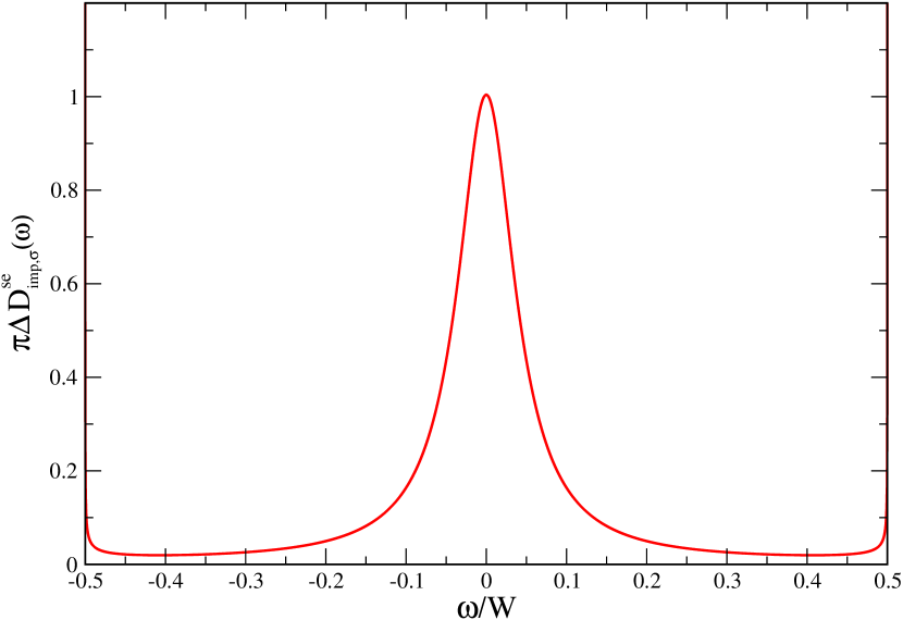
Figure 2: Impurity spectral function for a semi-elliptic density of states at $V=0.1W$ ($W\equiv 1$). The dominant Lorentzian line-shape around $\omega=0$ turns into square-root divergences at the band edges.

6.2 Phase shift function and Friedel sum rule

In scattering theory, the phase shift function $\eta(\epsilon)$ and the excess density of states are related by [2]

$$\Delta\rho(\epsilon)=\frac{1}{\pi}\frac{\partial\eta(\epsilon)}{\partial\epsilon}$$ (96)

with the boundary condition $\eta(-\infty)=0$. In our case, $\Delta\rho(\epsilon)=D_{{\rm imp},\sigma}(\epsilon)$ and we see from equations (54), (93) that

$$\eta(\epsilon)=\frac{\pi}{2}+\tan^{-1}\left[\frac{\epsilon-\Lambda_{V}(\epsilon)}{\pi|V(\epsilon)|^{2}\rho_{0}(\epsilon)}\right]\;.$$ (97)

This equation shows that the Friedel sum-rule is fulfilled, $\eta(E_{\rm F})=(\pi/2)n_{\rm d}$, where $E_{\rm F}=0$ is the Fermi energy and $n_{\rm d}=2n_{{\rm d},\sigma}=1$ is the impurity occupancy at half band-filling.

6.3 Impurity spectral function

For non-interacting electrons, the $d$-electron Green function is readily calculated from the Lehmann representation (25). For $\hat{A}=\hat{d}_{\sigma}^{\vphantom{+}}$ and $\hat{B}=\hat{d}_{\sigma}^{+}$ only the eigenstates $|\psi_{m}^{\rm p}\rangle=\hat{a}_{m,\sigma}^{+}|\psi_{0}\rangle$ and $|\psi_{m}^{\rm h}\rangle=\hat{a}_{m,\sigma}^{\vphantom{+}}|\psi_{0}\rangle$ contribute. We use for a particle excitation $E_{m}^{\rm p}=E(m)+E_{0}$

$$\langle\psi_{0}|\hat{d}_{\sigma}^{\vphantom{+}}\hat{a}_{m,\sigma}^{+}|\psi_{0}\rangle=\langle\psi_{0}|\left[\hat{d}_{\sigma}^{\vphantom{+}},\hat{a}_{m,\sigma}^{+}\right]_{+}|\psi_{0}\rangle=g_{m}^{*}\;,$$ (98)

and likewise for a hole excitation with $E_{m}^{\rm h}=-E(m)+E_{0}$ to find

$$\tilde{G}_{d,d}^{\rm ret}(\omega)=\frac{1}{L}\sum_{m}\frac{|g(E(m))|^{2}}{\omega-E(m)+{\rm i}\eta}$$ (99)

for the retarded $d$-electron Green function. It is the sum over poles in the lower complex plane at the exact excitation energies $E(m)$ with weight $|g_{m}|^{2}$.

The corresponding impurity spectral function follows from the definition (27) as

$$D_{d,d}(\omega)=\frac{1}{L}\sum_{m}|g(E(m))|^{2}\delta(\omega-E(m))\;.$$ (100)

To get further insight into the spectral function, we reconsider the eigenenergy equation (39),

$$E(m) = \widetilde{\Lambda}_{V}(E(m))\;,$$

$$\widetilde{\Lambda}_{V}(\omega) = \frac{1}{L}\sum_{p}\frac{|V_{p}|^{2}}{\omega-\epsilon(p)}\;,$$

$$\widetilde{\Lambda}_{V}^{\prime}(\omega) = -\left(\frac{1}{|g(\omega)|^{2}}-1\right)\;,$$ (101)

where we used equation (40). In the vicinity of an eigenenergy $E(m)=\widetilde{\Lambda}_{V}(E(m))$ we Taylor expand

$$\omega-\widetilde{\Lambda}_{V}(\omega) \approx E(m)+(\omega-E(m))$$ (102)

$$-\widetilde{\Lambda}_{V}(E(m))-\widetilde{\Lambda}_{V}^{\prime}(E(m))(\omega-E(m))\;,$$

so that

$$\frac{1}{\omega-\widetilde{\Lambda}_{V}(\omega)}=\frac{1}{1-\widetilde{\Lambda}_{V}^{\prime}(E(m))}\frac{1}{\omega-E(m)}=\frac{|g_{m}|^{2}}{\omega-E(m)}\;,$$ (103)

where we used equations (100) and (101). Therefore, we can equally write

$$D_{d,d}(\omega)=-\frac{1}{\pi}{\rm Im}\left(\frac{1}{\omega-\widetilde{\Lambda}_{V}(\omega)}\right)$$ (104)

for the impurity density of states. With the help of equation (69) we can explicitly evaluate equation (100) in the thermodynamic limit,

$$D_{d,d}(\omega) = \int_{-1/2}^{1/2}{\rm d}\epsilon\rho_{0}(\epsilon)|g(\epsilon)|^{2}\delta(\epsilon-\omega)$$ (105)

$$= \frac{\rho_{0}(\omega)|V(\omega)|^{2}}{(\pi\rho_{0}(\omega)|V(\omega)|^{2})^{2}+(\omega-\Lambda_{V}(\omega))^{2}}\;,$$

which is the well-known result for the impurity spectral function for the non-interacting single-impurity Anderson model.

7 Conclusions

In this work we started from the eigenvalue equations to derive ground-state properties for the non-interacting symmetric single-impurity Anderson model. We derived the ground-state energy, the hybridization and momentum distribution functions, and various spectral functions such as the density of states, the phase-shift function and the impurity spectral function. For comparison, in the supplementary material we used the standard equation-of-motion approach to derive the Green functions and ground-state expectation values.

For a finite host bandwidth $W$, we demonstrate that the impurity spectral function can display a finite weight at the band edges. For a semi-elliptic density of states and a constant hybridization, we give an explicit expression for the impurity spectral function for all hybridization strengths $V<W/4$, where no bound and anti-bound states exists. The usual Lorentzian spectrum is recovered in the weak-hybridization limit, $V/W\to 0$.

Our work closes a gap in the analytical treatment of the single-impurity Anderson model. Moreover, our explicit expressions for ground-state expectation values will be useful for variational approaches such as the Gutzwiller wave function.

8 Supporting information

In the supporting information, we derive the Green functions for the non-interacting single-impurity Green function from the equation-of-motion method. Using the Green functions, we calculate the total density of states and ground-state expectation values. The results agree with those obtained from the direct calculations in the previous sections.

8.1 Equation-of-motion approach

8.1.1 Time domain

We study the four retarded Green functions

$$G_{k,p}^{\rm ret}(t) = (-{\rm i})\Theta(t)\langle\left[\hat{c}_{k,\sigma}^{\vphantom{+}}(t),\hat{c}_{p,\sigma}^{+}\right]_{+}\rangle\;,$$ (106)

$$G_{d,p}^{\rm ret}(t) = (-{\rm i})\Theta(t)\langle\left[\hat{d}_{\sigma}^{\vphantom{+}}(t),\hat{c}_{p,\sigma}^{+}\right]_{+}\rangle\;,$$ (107)

$$G_{k,d}^{\rm ret}(t) = (-{\rm i})\Theta(t)\langle\left[\hat{c}_{k,\sigma}^{\vphantom{+}}(t),\hat{d}_{\sigma}^{+}\right]_{+}\rangle\;,$$ (108)

$$G_{d,d}^{\rm ret}(t) = (-{\rm i})\Theta(t)\langle\left[\hat{d}_{\sigma}^{\vphantom{+}}(t),\hat{d}_{\sigma}^{+}\right]_{+}\rangle\;,$$ (109)

Taking the time derivative leads to

$${\rm i}\dot{G}^{\rm ret}_{k,p}(t) = \delta(t)\delta_{k,p}+(-{\rm i})\Theta(t)\langle\left[\left[\hat{c}_{k,\sigma}^{\vphantom{+}}(t),\hat{H}_{0}\right]_{-},\hat{c}_{p,\sigma}^{+}\right]_{+}\rangle$$ (110)

$$= \delta(t)\delta_{k,p}+\epsilon(k)G_{k,p}^{\rm ret}(t)+\frac{V_{k}^{*}}{\sqrt{L}}G_{d,p}^{\rm ret}(t)\;,$$

$${\rm i}\dot{G}_{d,p}^{\rm ret}(t) = (-{\rm i})\Theta(t)\langle\left[\left[\hat{d}_{\sigma}^{\vphantom{+}}(t),\hat{H}_{0}\right]_{-},\hat{c}_{p,\sigma}^{+}\right]_{+}\rangle$$ (111)

$$= \sum_{k}\frac{V_{k}}{\sqrt{L}}G_{k,p}^{\rm ret}(t)\;,$$

$${\rm i}\dot{G}_{k,d}^{\rm ret}(t) = (-{\rm i})\Theta(t)\langle\left[\left[\hat{c}_{k,\sigma}^{\vphantom{+}}(t),\hat{H}_{0}\right]_{-},\hat{d}_{\sigma}^{+}\right]_{+}\rangle$$ (112)

$$= \epsilon(k)G_{k,d}^{\rm ret}(t)+\frac{V_{k}^{*}}{\sqrt{L}}G_{d,d}^{\rm ret}(t)\;,$$

$${\rm i}\dot{G}_{d,d}^{\rm ret}(t) = \delta(t)+(-{\rm i})\Theta(t)\langle\left[\left[\hat{d}_{\sigma}^{\vphantom{+}}(t),\hat{H}_{0}\right]_{-},\hat{d}_{\sigma}^{+}\right]_{+}\rangle$$ (113)

$$= \delta(t)+\sum_{k}\frac{V_{k}}{\sqrt{L}}G_{k,d}^{\rm ret}(t)\;.$$

Here, we used the anticommutation relations of the Fermi operators and the commutation relations

$$\left[\hat{c}_{k,\sigma}^{\vphantom{+}},\hat{T}\right]_{-}=\epsilon(k)\hat{c}_{k,\sigma}^{\vphantom{+}} \;,\; \left[\hat{d}_{\sigma}^{\vphantom{+}},\hat{T}\right]_{-}=0\;,$$

$$\left[\hat{c}_{k,\sigma}^{\vphantom{+}},\hat{V}\right]_{-}=\frac{V_{k}^{*}}{\sqrt{L}}\hat{d}_{\sigma}^{\vphantom{+}} \left[\hat{d}_{\sigma}^{\vphantom{+}},\hat{V}\right]_{-}=\sum_{k}\frac{V_{k}}{\sqrt{L}}\hat{c}_{k,\sigma}^{\vphantom{+}}\;.$$ , (114)

For non-interacting electrons, the equations of motion lead to a closed set of differential equations (110)–(113).

8.1.2 Fourier transformation of time derivatives

The equation-of-motion method works in the frequency domain. The Fourier transformation of the time derivative of retarded Green functions are given by

$${\rm FT}\left\{{\rm i}\dot{G}_{A,B}^{\rm ret}(t)\right\}(\omega) = \int_{-\infty}^{\infty}{\rm d}te^{-\eta|t|}e^{{\rm i}\omega t}\left({\rm i}\dot{G}_{A,B}(t)\right)$$ (115)

$$= {\rm i}\biggl{[}\left.G_{A,B}^{\rm ret}(t)e^{-\eta|t|}e^{{\rm i}\omega t}\right|_{-\infty}^{\infty}$$

$$-\int_{0}^{\infty}{\rm d}tG_{A,B}^{\rm ret}(t)\frac{{\rm d}}{{\rm d}t}\left(e^{-\eta t}e^{{\rm i}\omega t}\right)\biggr{]}$$

$$= (\omega+{\rm i}\eta)\int_{-\infty}^{\infty}{\rm d}tG_{A,B}^{\rm ret}(t)e^{-\eta|t|}e^{{\rm i}\omega t}$$

$$= (\omega+{\rm i}\eta)\tilde{G}_{A,B}^{\rm ret}(\omega)\;,$$

where we used partial integration in the first step and the fact that $G_{A,B}^{\rm ret}(t<0)=0$.

The Fourier transformation of a Green function’s time derivative can also be done using contour integration. By definition of the Fourier transformation, we have

$${\rm i}\dot{G}_{A,B}^{\rm ret}(t)=\int_{-\infty}^{\infty}\frac{{\rm d}\lambda}{2\pi}e^{-\eta_{2}|\lambda|}e^{-{\rm i}\lambda t}\lambda\tilde{G}_{A,B}^{\rm ret}(\lambda)\;.$$ (116)

To find the Fourier transformation of the left-hand side we multiply both sides with ${\rm exp}(-\eta t+{\rm i}\omega t)$ and integrate over $t$ from zero to infinity. Thus,

$${\rm FT}\Bigl{\{}{\rm i}\dot{G}_{A,B}^{\rm ret}(t)\Bigr{\}}(\omega) = \int_{-\infty}^{\infty}\frac{{\rm d}\lambda}{2\pi}e^{-\eta_{2}|\lambda|}\lambda\tilde{G}_{A,B}^{\rm ret}(\lambda)$$

$$\times\int_{0}^{\infty}{\rm d}te^{-{\rm i}\lambda t}e^{{\rm i}\omega t-\eta t}$$

$$= \int_{-\infty}^{\infty}\frac{{\rm d}\lambda}{2\pi{\rm i}}\tilde{G}_{A,B}^{\rm ret}(\lambda)e^{-\eta_{2}|\lambda|}\frac{\lambda}{\lambda-\omega-{\rm i}\eta}$$

$$= (\omega+{\rm i}\eta)\int_{-\infty}^{\infty}\frac{{\rm d}\lambda}{2\pi{\rm i}}\frac{\tilde{G}_{A,B}^{\rm ret}(\lambda)e^{-\eta_{2}|\lambda|}}{\lambda-\omega-{\rm i}\eta}\;,$$

where we used the fact that $G^{\rm ret}_{A,B}(t=0^{-})=0$ in the last step. Now that $\tilde{G}_{A,B}^{\rm ret}(\lambda)$ has only poles in the lower half of the complex plane, we extend the integral over the real axis in equation (LABEL:eq:FTrealaxis) to a contour integral with an arc of infinite radius in the upper half of the complex plane. Since $G_{A,B}^{\rm ret}(\omega)\sim 1/\omega$ as seen from the Lehmann representation, the arc does not give a finite contribution. Then, the integral can be evaluated using the residue theorem. The pole of strength unity at $\lambda=\omega+{\rm i}\eta$ gives, letting $\eta_{2}=0$, $\eta=0$ where appropriate,

$${\rm FT}\left\{{\rm i}\dot{G}_{A,B}^{\rm ret}(t)\right\}(\omega)=(\omega+{\rm i}\eta)\tilde{G}_{A,B}^{\rm ret}(\omega)\;,$$ (118)

and we recover equation (115).

8.1.3 Explicit solution in the frequency domain

To solve the equations (110)–(113) we transformation them into frequency space. We find

$$\left(\omega+{\rm i}\eta\right)\tilde{G}_{k,p}^{\rm ret}(\omega) = \delta_{k,p}+\epsilon(k)\tilde{G}_{k,p}^{\rm ret}(\omega)+\frac{V_{k}^{*}}{\sqrt{L}}\tilde{G}_{d,p}^{\rm ret}(\omega)\;,$$

$$\left(\omega+{\rm i}\eta\right)\tilde{G}_{d,p}^{\rm ret}(\omega) = \sum_{k}\frac{V_{k}}{\sqrt{L}}\tilde{G}_{k,p}^{\rm ret}(\omega)\;,$$ (120)

$$\left(\omega+{\rm i}\eta\right)\tilde{G}_{k,d}^{\rm ret}(\omega) = \epsilon(k)\tilde{G}_{k,d}^{\rm ret}(\omega)+\frac{V_{k}^{*}}{\sqrt{L}}\tilde{G}_{d,d}^{\rm ret}(\omega)\;,$$ (121)

$$\left(\omega+{\rm i}\eta\right)\tilde{G}_{d,d}^{\rm ret}(\omega) = 1+\sum_{k}\frac{V_{k}}{\sqrt{L}}\tilde{G}_{k,d}^{\rm ret}(\omega)\;.$$ (122)

Since we have obtained algebraic equations as a function of $\omega$, we are now in the position to transform the retarded to the causal Green function, i.e., the equations of motion for the causal Green function in frequency space are obtained by replacing $\eta$ by $\eta{\rm sgn}(\omega)$ in eqs. (LABEL:eq:GFdot1om)–(122).

The resulting set of equations is readily solved. We define the retarded and causal hybridization functions

$$\Delta^{\rm ret}(\omega) = \frac{1}{L}\sum_{k}\frac{|V_{k}|^{2}}{\omega-\epsilon(k)+{\rm i}\eta}\;,$$

$$\Delta^{\rm c}(\omega) = \frac{1}{L}\sum_{k}\frac{|V_{k}|^{2}}{\omega-\epsilon(k)+{\rm i}\eta{\rm sgn}(\omega)}\;,$$ (123)

and find

$$\tilde{G}_{k,p}^{\rm c}(\omega) = \frac{1}{\omega-\epsilon(k)+{\rm i}\eta{\rm sgn}(\omega)}\biggl{(}\delta_{k,p}$$

$$+\frac{1}{L}\frac{V_{p}V_{k}^{*}}{(\omega-\epsilon(p)+{\rm i}\eta{\rm sgn}(\omega))(\omega-\Delta^{\rm c}(\omega))}\biggr{)}\;,$$

$$\tilde{G}_{d,p}^{\rm c}(\omega)=\sqrt{\frac{1}{L}}\frac{V_{p}}{(\omega-\epsilon(p)+{\rm i}\eta{\rm sgn}(\omega))(\omega-\Delta^{\rm c}(\omega))}\;,$$ (125)

$$\tilde{G}_{k,d}^{\rm c}(\omega)=\sqrt{\frac{1}{L}}\frac{V_{k}^{*}}{(\omega-\epsilon(k)+{\rm i}\eta{\rm sgn}(\omega))(\omega-\Delta^{\rm c}(\omega))}\;,$$ (126)

and

$$\tilde{G}_{d,d}^{\rm c}(\omega)=\frac{1}{\omega-\Delta^{\rm c}(\omega)}\;.$$ (127)

The equations for the retarded Green functions are obtained by replacing $\eta{\rm sgn}(\omega)$ by $\eta$.

8.2 Spectral properties

8.2.1 Impurity spectral function

First, we re-derive the impurity spectral function from the impurity Green function (127). We have

$$\Delta^{\rm ret}(\omega) = \int_{-1/2}^{1/2}{\rm d}\epsilon\frac{\rho_{0}(\epsilon)|V(\epsilon)|^{2}}{\omega-\epsilon+{\rm i}\eta}$$ (128)

$$= \Lambda_{V}(\epsilon)-{\rm i}\pi\rho_{0}(\omega)|V(\omega)|^{2}\;.$$

The definition of the spectral function immediately gives

$$D_{d,d}(\omega) = -\frac{1}{\pi}{\rm Im}\left(\frac{1}{\omega-\Delta^{\rm ret}(\omega)}\right)$$ (129)

$$= \frac{\rho_{0}(\omega)|V(\omega)|^{2}}{(\pi\rho_{0}(\omega)|V(\omega)|^{2})^{2}+(\omega-\Lambda_{V}(\omega))^{2}}\;,$$

as derived in Sect. 6.

8.2.2 Density of states

We write the density of states in the form

$$D_{\sigma}(\omega) = -\frac{1}{\pi}{\rm Im}\biggl{(}\sum_{m}\langle\hat{a}_{m,\sigma}^{+}\frac{1}{\omega-(\hat{H}_{0}-E_{0})+{\rm i}\eta}\hat{a}_{m,\sigma}^{\vphantom{+}}\rangle$$ (130)

$$\hphantom{-\frac{1}{\pi}}+\langle\hat{a}_{m,\sigma}^{\vphantom{+}}\frac{1}{\omega-(\hat{H}_{0}-E_{0})+{\rm i}\eta}\hat{a}_{m,\sigma}^{+}\rangle\biggr{)}\,,$$

where we used the fact that $\hat{a}_{m,\sigma}^{+}$ ($\hat{a}_{m,\sigma}^{\vphantom{+}}$) creates (annihilates) an electron with energy $E(m)$ in the ground state. The sum over all $m$ runs over all single-particle excitations of the ground state and thus represents the trace over all single-particle eigenstates,

$$D_{\sigma}(\omega)=-\frac{1}{\pi}{\rm Im}{\rm Tr}_{1}\Bigl{(}\frac{1}{\omega-(\hat{H}_{0}-E_{0})+{\rm i}\eta}\Bigr{)}\;.$$ (131)

We can equally use the excitations $\hat{c}_{k,\sigma}^{+}|\psi_{0}\rangle$, $\hat{c}_{k,\sigma}^{\vphantom{+}}|\psi_{0}\rangle$, and $\hat{d}_{\sigma}^{+}|\psi_{0}\rangle$, $\hat{d}_{\sigma}^{\vphantom{+}}|\psi_{0}\rangle$, respectively, to perform the trace over the single-particle excitations of the ground state. Therefore, we may write

$$D_{\sigma}(\omega) = -\frac{1}{\pi}{\rm Im}\biggl{[}\sum_{k}\biggl{(}\langle\hat{c}_{k,\sigma}^{+}\frac{1}{\omega-(\hat{H}_{0}-E_{0})+{\rm i}\eta}\hat{c}_{k,\sigma}^{\vphantom{+}}\rangle$$ (132)

$$\hphantom{-\frac{1}{\pi}{\rm Im}\biggl{(}\sum_{k}}+\langle\hat{c}_{k,\sigma}^{\vphantom{+}}\frac{1}{\omega-(\hat{H}_{0}-E_{0})+{\rm i}\eta}\hat{c}_{k,\sigma}^{+}\rangle\biggr{)}$$

$$\hphantom{-\frac{1}{\pi}{\rm Im}\biggl{(}}+\langle\hat{d}_{\sigma}^{+}\frac{1}{\omega-(\hat{H}_{0}-E_{0})+{\rm i}\eta}\hat{d}_{\sigma}^{\vphantom{+}}\rangle$$

$$\hphantom{-\frac{1}{\pi}{\rm Im}\biggl{(}}+\langle\hat{d}_{\sigma}^{\vphantom{+}}\frac{1}{\omega-(\hat{H}_{0}-E_{0})+{\rm i}\eta}\hat{d}_{\sigma}^{+}\rangle\biggr{]}$$

$$= -\frac{1}{\pi}{\rm Im}\biggl{[}\sum_{k}G_{k,k}^{\rm ret}(\omega)+G_{d,d}^{\rm ret}(\omega)\biggr{]}\;.$$

Equation (LABEL:eq:EOMimpurityGF1) shows that the band Green function consists of the undisturbed host Green function for $V_{k}\equiv 0$ and a $1/L$ correction due to the hybridization. Therefore, using eqs. (LABEL:eq:EOMimpurityGF1) and (127), the contribution due to a finite hybridization is given by

$$D_{{\rm imp},\sigma}(\omega) = -\frac{1}{\pi}{\rm Im}\biggl{[}\frac{1}{\omega-\Delta^{\rm ret}(\omega)}$$ (133)

$$\hphantom{-\frac{1}{\pi}{\rm Im}}\times\left(1+\sum_{k}\frac{|V_{k}|^{2}/L}{(\omega-\epsilon(k)+{\rm i}\eta)^{2}}\right)\biggr{]}$$

$$= -\frac{1}{\pi}{\rm Im}\left[\frac{1-(\partial\Delta^{{\rm ret}}(\omega))/(\partial\omega)}{\omega-\Delta^{\rm ret}(\omega)}\right]$$

$$= -\frac{1}{\pi}\frac{\partial}{\partial\omega}{\rm Im}\left[\ln\left(\omega-\Delta^{\rm ret}(\omega)\right)\right]\;.$$

We use equation (128) and find from the complex logarithm

$$D_{{\rm imp},\sigma}(\omega) = -\frac{1}{\pi}\frac{\partial}{\partial\omega}\left[\tan^{-1}\left(\frac{\pi\rho_{0}(\omega)|V(\omega)|^{2}}{\omega-\Lambda_{V}(\omega)}\right)\right]$$ (134)

$$= \frac{\partial}{\partial\omega}\left[\rho_{0}(\omega)y(\omega)\right]\;,$$

as derived in Sect. 6.

8.3 Ground-state expectation values

Lastly, we re-derive the ground-state expectation values for the $d$-occupancy, the hybridization matrix element, and the momentum distribution from the Green function approach.

8.3.1 Expectation values from Green functions

The Green functions permit the calculation of ground-state expectation values. By definition, we have ($\eta=0^{+}$)

$$\langle\hat{B}\hat{A}\rangle = (-{\rm i})G_{A,B}(t=-\eta)$$ (135)

$$= \int_{-\infty}^{\infty}\frac{{\rm d}\omega}{2\pi{\rm i}}e^{-\eta_{2}|\omega|}e^{{\rm i}\eta\omega}\tilde{G}_{A,B}^{\rm c}(\omega)\;.$$

We extend the integral over the real axis into a contour integral in the complex plane where the closed contour $C$ runs over the real axis and an arc with infinite radius in the upper complex plane. Due to the factor $\exp[{\rm i}\eta({\rm Re}(z)+{\rm i}{\rm Im}(z)]$, the arc does not contribute because ${\rm Im}(z)\to+\infty$ on the arc. Therefore, we have

$$\langle\hat{B}\hat{A}\rangle=\oint_{C}\frac{{\rm d}z}{2\pi{\rm i}}\tilde{G}_{A,B}^{\rm c}(z)e^{{\rm i}z\eta}\;.$$ (136)

It is not always easy to do the integral because the Green functions display branch cuts in the complex plane.

8.3.2 Ground-state energy

The ground-state energy can immediately be calculated using the density of states,

$$\frac{\Delta E}{2}=\int_{-1/2}^{0}{\rm d}\omega\omega D_{{\rm imp},\sigma}(\omega)\;.$$ (137)

The result for the impurity density of states (134) and a partial integration directly lead to the desired result for the ground-state energy.

8.3.3 Impurity occupancy

For the $d$-electron occupancy, $\hat{A}=\hat{d}_{\sigma}^{\vphantom{+}}$, $\hat{B}=\hat{d}_{\sigma}^{+}$, we find

$$\langle\hat{d}_{\sigma}^{+}\hat{d}_{\sigma}^{\vphantom{+}}\rangle=\oint_{C}\frac{{\rm d}z}{2\pi{\rm i}}e^{{\rm i}\eta z}\frac{1}{z-\Delta^{\rm c}(z)}\;.$$ (138)

$\Delta^{\rm c}(z)$ has a branch cut on the real axis that is infinitesimally above the real axis for ${\rm Re}(z)=\omega<0$ and infinitesimally below the real axis for $\omega>0$. Since $1/(z-\Delta^{\rm c}(z))$ is otherwise analytic in the complex plane, we can deform the contour $C$ to $\tilde{C}$ where $\tilde{C}$ encloses the branch cut for $-1/2<\omega<0$ at infinitesimal distance $\xi$. The corners of $\tilde{C}$ provide a vanishingly small contribution and only the integrals below and above the branch cut remain finite for $\xi\to 0$,

$$\langle\hat{d}_{\sigma}^{+}\hat{d}_{\sigma}^{\vphantom{+}}\rangle = \oint_{\tilde{C}}\frac{{\rm d}z}{2\pi{\rm i}}\frac{1}{z-\Delta^{\rm c}(z)}$$

$$= \int_{-1/2}^{0}\frac{{\rm d}\omega}{2\pi{\rm i}}\frac{1}{\omega-\Lambda_{V}(\omega)-{\rm i}\rho_{0}(\omega)|V(\omega)|^{2}}$$

$$+\int_{0}^{-1/2}\frac{{\rm d}\omega}{2\pi{\rm i}}\frac{1}{\omega-\Lambda_{V}(\omega)+{\rm i}\rho_{0}(\omega)|V(\omega)|^{2}}\;,$$

where we used

$$\Delta^{\rm c}(\omega-{\rm i}\xi) = \Lambda_{V}(\omega)+{\rm i}\pi\rho_{0}(\omega)|V(\omega)|^{2}\;,$$

$$\Delta^{\rm c}(\omega+{\rm i}\xi) = \Lambda_{V}(\omega)-{\rm i}\pi\rho_{0}(\omega)|V(\omega)|^{2}$$ (140)

infinitesimally below and above the branch cut. From equation (LABEL:eq:GFdoccupancy) we readily recover $\langle\hat{d}_{\sigma}^{+}\hat{d}_{\sigma}^{\vphantom{+}}\rangle=1/2$.

8.3.4 Hybridization

The derivation of the hybridization matrix element proceeds along the same lines. We have

$$\langle\hat{c}_{k,\sigma}^{+}\hat{d}_{\sigma}^{\vphantom{+}}\rangle=\oint_{C}\frac{{\rm d}z}{2\pi{\rm i}}\frac{1}{z-\epsilon(k)+{\rm i}{\rm sgn}(\epsilon(k))}\frac{1}{z-\Delta^{\rm c}(z)}\;.$$ (141)

For $0<\epsilon(k)<1/2$, there is a pole in the lower complex plane that does not give a contribution to the contour integral. Following the same lines as for the impurity occupancy we thus find

$$\langle\hat{c}_{k,\sigma}^{+}\hat{d}_{\sigma}^{\vphantom{+}}\rangle = \frac{V_{k}}{\sqrt{L}}\int_{-1/2}^{0}{\rm d}\omega\frac{1}{\omega-\epsilon(k)}$$ (142)

$$\hphantom{\frac{V_{k}}{\sqrt{L}}}\times\frac{\rho_{0}(\omega)|V(\omega)|^{2}}{[\omega-\Lambda_{V}(\omega)]^{2}+[\pi\rho_{0}(\omega)|V(\omega)|^{2}]^{2}}$$

$$= \frac{V_{k}}{\sqrt{L}}H(\epsilon(k))$$

for $\epsilon(k)>0$ with $H(\epsilon)$ from the main text. This contribution is also present for $-1/2<\epsilon(k)<0$ but the integral must be understood as principal value integral to circumvent the singularity at $\omega=\epsilon(k)$. For $-1/2<\epsilon(k)<0$, our contour $\tilde{C}$ also encloses the pole at $z=\epsilon+{\rm i}\eta$. The pole contributes at the real value $\omega=\epsilon(k)$, i.e., on the branch cut itself where

$${\rm Re}\left(\frac{1}{\omega-\Delta^{\rm c}(\omega)}\right)=\frac{\omega-\Lambda_{V}(\omega)}{[\omega-\Lambda_{V}(\omega)]^{2}+[\pi\rho_{0}(\omega)|V(\omega)|^{2}]^{2}}\;.$$ (143)

Thus, we find

$$\langle\hat{c}_{k,\sigma}^{+}\hat{d}_{\sigma}^{\vphantom{+}}\rangle = \frac{V_{k}}{\sqrt{L}}H(\epsilon(k))$$ (144)

$$+\frac{(V_{k}/\sqrt{L})\rho_{0}(\epsilon(k))|V(\epsilon(k))|^{2}}{[\epsilon(k)-\Lambda_{V}(\epsilon(k))]^{2}+[\pi\rho_{0}(\epsilon(k))|V(\epsilon(k))|^{2}]^{2}}$$

$$= \frac{V_{k}}{\sqrt{L}}\left[H(\epsilon(k))+G(\epsilon(k))\right]$$

for $\epsilon(k)<0$ with $G(\epsilon)$ from Sect. 5.

8.3.5 Momentum distribution

The calculation of the momentum distribution $n_{k,\sigma}=n_{k,\sigma}^{(0)}+n_{k,\sigma}^{(1)}/L$ requires the elementary integral

$$n_{k,\sigma}^{(0)}=\oint_{C}\frac{{\rm d}z}{2\pi{\rm i}}e^{{\rm i}\eta z}\frac{1}{z-\epsilon(k)+{\rm i}{\rm sgn}(\epsilon(k))}=\Theta(-\epsilon(k))\;.$$ (145)

Here, we used the fact that there is a pole in the upper complex plane of strength unity for $\epsilon(k)<0$ only. Moreover,

$$n_{k,\sigma}^{(1)} = |V_{k}|^{2}\int_{-\infty}^{\infty}\frac{{\rm d}\omega}{2\pi{\rm i}}e^{{\rm i}\eta\omega}\frac{1}{\omega-\Delta^{\rm c}(\omega)}$$ (146)

$$\hphantom{|V_{k}|^{2}\int_{-\infty}^{\infty}}\times\frac{1}{[\omega-\epsilon(k)+{\rm i}\eta{\rm sgn}(\omega)]^{2}}$$

$$= |V_{k}|^{2}\frac{\partial}{\partial\epsilon(k)}\left[G(\epsilon(k))+H(\epsilon(k))\right]$$

$$= |V_{k}|^{2}\left[G^{\prime}(\epsilon(k))+H^{\prime}(\epsilon(k))\right]\;,$$

as derived in Sect. 5.

- [1] P. W. Anderson, Phys. Rev. 124, 41 (1961).
- [2] A. C. Hewson, The Kondo Problem to Heavy Fermions, Cambridge Studies in Magnetism, Vol. 2 (Cambridge University Press, Cambridge, 1997).
- [3] J. Sólyom, Fundamentals of the Physics of Solids, Vol. 3 (Springer, Heidelberg, 2010).
- [4] K. Schönhammer, Phys. Rev. B 42, 2591 (1990).
- [5] F. Gebhard, Phys. Rev. B 44, 992 (1991).
- [6] I. S. Gradshteyn and I. M. Ryzhik, Table of Integrals, Series and Products, eighth edition, ed. by D. Zwillinger and V. Moll (Academic Press, Amsterdam, 2015).
- [7] J. von Delft and H. Schoeller, Ann. Phys. 7, 225–305 (1998).