A Characteristic Transmission Spectrum dominated by H₂O applies to the majority of HST/WFC3 exoplanet observations

Abstract

Currently, 19 transiting exoplanets have published transmission spectra obtained with the Hubble/WFC3 G141 near-IR grism. Using this sample, we have undertaken a uniform analysis incorporating measurement-error debiasing of the spectral modulation due to H₂O, measured in terms of the estimated atmospheric scale height, ${H_{s}}$. For those planets with a reported H₂O detection (10 out of 19), the spectral modulation due to H₂O ranges from 0.9 to 2.9 ${H_{s}}$ with a mean value of 1.8 $\pm$ 0.5 ${H_{s}}$. This spectral modulation is significantly less than predicted for clear atmospheres. For the group of planets in which H₂O has been detected, we find the individual spectra can be coherently averaged to produce a characteristic spectrum in which the shape, together with the spectral modulation of the sample, are consistent with a range of H₂O mixing ratios and cloud-top pressures, with a minimum H₂O mixing ratio of 17 ${}^{+12}_{-6}$ ppm corresponding to the cloud-free case. Using this lower limit, we show that clouds or aerosols must block at least half of the atmospheric column that would otherwise be sampled by transmission spectroscopy in the case of a cloud-free atmosphere. We conclude that terminator-region clouds, with sufficient opacity to be opaque in slant-viewing geometry, are common in hot Jupiters.

1. Introduction

The search for H₂O in exoplanet atmospheres has been dominated by transmission measurements obtained with space-based instruments. Although the early detections of H₂O in an exoplanet atmosphere were made with the Hubble and Spitzer instruments STIS, IRAC, and NICMOS (Barman, 2008; Tinetti et al., 2007; Swain et al., 2008; Grillmair et al., 2008), the leading instrument in this area is NASA’s Hubble Space Telescope (HST) Wide Field Camera 3 (WFC3) using the G141 IR grism (1.1–1.7 $\mu$m), to obtain spectra of the transit event. The scope of the collective work is impressive and constitutes the largest collection, 19, of similarly-observed exoplanets presently available. These 19 transmission spectra are drawn from 16 papers by 13 authors, a majority (10 of 19) of which report a detection of H₂O (Table 1; Deming et al., 2013; Ehrenreich et al., 2014; Fraine et al., 2014; Huitson et al., 2013; Knutson et al., 2014a, b; Kreidberg et al., 2014a, b, 2015; Line et al., 2013b; Mandell et al., 2013; McCullough et al., 2014; Ranjan et al., 2014; Sing et al., 2015; Wakeford et al., 2013; Wilkins et al., 2014). As a whole, this sample represents a heterogeneous collection of data reduction methods, spectral resolution, observational, and model interpretation approaches. Given these differences, we focus our analysis on the H₂O absorption feature, which occurs in the near-infrared at $\sim$ 1.2–1.6  $\mu$m. Here we report the trends for both spectral modulation and spectral shape and discuss the possible implications of these findings.

2. Methods

Table 1HST/WFC3 IR exoplanet transmission observations used in this analysis

Object	Teff	Planetary	Derived Spectral	Derived Spectral	Spectral
Name	Calculated (K)	Scale Height (km)	Modulation (ppm)	Modulation (Hs)	Channels	Source
H2O-detection Reported
HAT-P-1b	1304$\pm 40$	544$\pm 58$	430$\pm 178$	2.8$\pm 1.2$	28	Wakeford et al. (2013)
HAT-P-11b	870$\pm 16$	269$\pm 33$	127$\pm 47$	2.2$\pm 0.8$	29	Fraine et al. (2014)
HD 189733b	1199$\pm 21$	197$\pm 14$	222$\pm 63$	2.0$\pm 0.6$	28	McCullough et al. (2014)
HD 209458b	1445$\pm 19$	558$\pm 25$	241$\pm 38$	1.5$\pm 0.2$	28	Deming et al. (2013)
WASP-12b	2581$\pm 90$	951$\pm 106$	280$\pm 21$	1.5$\pm 0.1$	8	Kreidberg et al. (2015)
WASP-17b	1546$\pm 58$	1000$\pm 152$	587$\pm 232$	1.5$\pm 0.6$	19	Mandell et al. (2013)
WASP-19b	2064$\pm 46$	502$\pm 29$	306$\pm 86$	1.5$\pm 0.4$	6	Huitson et al. (2013)
WASP-31b	1572$\pm 35$	1140$\pm 105$	359$\pm 270$	1.1$\pm 0.8$	25	Sing et al. (2015)
WASP-43b	1374$\pm 78$	97$\pm 15$	99$\pm 66$	1.4$\pm 0.9$	22	Kreidberg et al. (2014b)
XO-1b	1206$\pm 29$	275$\pm 31$	292$\pm 110$	2.7$\pm 1.0$	29	Deming et al. (2013)
Non-H2O-detection Reported
CoRoT-1b	1897$\pm 81$	598$\pm 95$	845$\pm 959$	4.1$\pm 4.6$	10	Ranjan et al. (2014)
CoRoT-2b	1537$\pm 39$	144$\pm 10$	95$\pm 77$	1.3$\pm 1.0$	11	Wilkins et al. (2014)
GJ 436b	649$\pm 58$	183$\pm 20$	49$\pm 44$	0.5$\pm 0.5$	28	Knutson et al. (2014a)
GJ 1214b	560$\pm 29$	226$\pm 46$	16$\pm 28$	0.0$\pm 0.1$	22	Kreidberg et al. (2014a)
GJ 3470b	651$\pm 55$	294$\pm 88$	3$\pm 31$	0.0$\pm 0.2$	107	Ehrenreich et al. (2014)
HAT-P-12b	957$\pm 17$	603$\pm 47$	0$\pm 373$	0.0$\pm 1.1$	23	Line et al. (2013b)
HD 97658b	733$\pm 23$	169$\pm 28$	22$\pm 18$	1.1$\pm 0.9$	28	Knutson et al. (2014b)
TrES-2b	1497$\pm 32$	269$\pm 22$	286$\pm 162$	3.0$\pm 1.7$	10	Ranjan et al. (2014)
TrES-4b	1784$\pm 40$	861$\pm 95$	524$\pm 451$	3.9$\pm 3.4$	10	Ranjan et al. (2014)

Given a heterogeneous collection of measurements presently, we adopt a template-fitting approach to determine the spectral modulation due to H₂O opacity. We define spectral modulation as the amplitude of the H₂O feature between 1.2–1.4 $\mu$m. We generate H₂O template spectra that include the opacities due to Rayleigh scattering and H₂/H₂ and H₂/He collisionally induced absorption, using the CHIMERA forward model routine for transmission spectra (Line et al., 2013a; Swain et al., 2014; Kreidberg et al., 2014b, 2015) over the spectral range of the G141 grism (1.1–1.7 $\micron$). These H₂O templates cover abundances from 0.1 to 100 ppm, the range over which the $shape$ of the H₂O spectral modulation changes. H₂O mixing ratios below 0.1 ppm are difficult to detect and abundances above 100 ppm produce spectra that have nearly the same shape when normalized. These templates are then fit to the HST/WFC3 data (Fig. 1) with a Levenburg-Markwardt least-squares minimization routine (e.g., Markwardt, 2009), by linearly scaling the model amplitudes and vertical offsets. This exercise is carried out in order to debias the estimate for spectral modulation from single point outliers and to create a consistent method to treat data reported spectral resolutions that differ by $\sim$5.

To facilitate further analysis, all of the HST/WFC3 data and their corresponding best-fit radiative transfer models are converted to units of planetary scale height $H_{s}$:

$$H_{s}=\frac{k_{B}T_{eq}}{\mu g}.$$ (1)

where $k_{B}$ is the Boltzmann constant, $\mu$ is the mean molecular weight of an atmosphere in solar composition ($\mu$ = 2.3 amu), $g$ is the surface gravity, and $T_{eq}$ is the calculated equilibrium temperature. We adopt the planetary parameters listed on exoplanets.org (Han et al., 2014) for all of these variables except the equilibrium temperature. Assuming efficient heat redistribution from the dayside to the nightside and an albedo of zero, we calculate the equilibrium temperature for each planet via the equation (Mendez, 2014):

$$T_{eq}=\frac{T_{*}{f^{{}^{\prime}\frac{1}{4}}}}{(a/R_{*})^{\frac{1}{2}}}\sqrt{1+\left(\frac{8}{\pi^{2}}-1\right)e^{\frac{5}{2}}}$$ (2)

where $T_{*}$ and $R_{*}$ are the stellar temperature and radius, $a$ is the semi-major axis, and $e$ is the eccentricity.

The modulation of each planet’s H₂O feature ($\sim$1.2–1.4 $\micron$) is determined by the amplitude of the best fit model template to prevent any outliers in each dataset from skewing the spectral fit. This parameter is then plotted versus the data uncertainty, defined as the mean uncertainty in each spectra scaled by the square root of the change in resolution. The error bars on the spectral modulation are defined as the standard deviation of the residuals of the best-fit template model, (Fig. 2) and all values here are in units of H_s.

The major outlying points of TrES-2b, TrES-4b and CoRoT-1b show a large uncertainty in their spectra as well as significant spectral modulation (Fig. 2). However, their poor fit to the water templates indicate that caution should be used in interpreting modulation results for these planets.

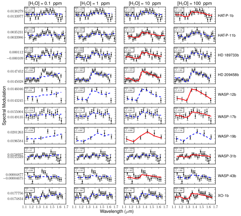
Figure 1.— The 10 published HST/WFC3 IR transmission spectra of exoplanets with a H₂O detection (black points; Table 1) are fit to a grid of cloud-free H₂O models with abundances of 0.1, 1, 10, and 100 ppm (blue dashed line) by scaling the models’ offsets and amplitudes. The standard deviation of the residuals (SDR) in units of scale height and the reduced chi squared ($\chi^{2}_{r}$) are noted for each case, where the minimum $\chi^{2}_{r}$ (as well as SDR) indicates the best-fit model for each target (solid red line). This analysis allows us to debias the estimate of the spectral modulation amplitude of the H₂O feature from outlying data points.

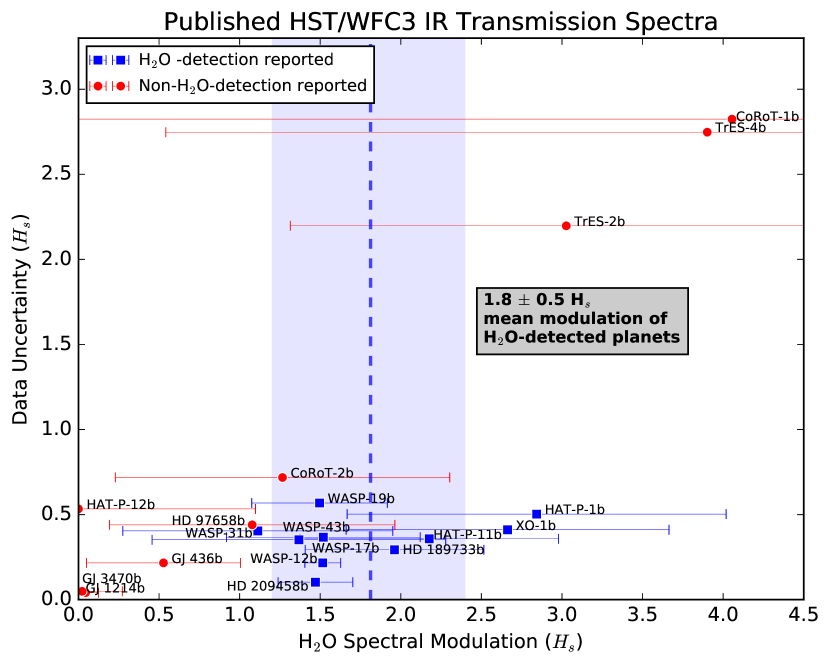
Figure 2.— The H₂O spectral modulation in scale heights of the 19 published HST/WFC3+G141 transiting exoplanet transmission spectra are plotted here versus the uncertainty of the data. The horizontal error bars are standard deviation of the residuals of the cloud-free H₂O model fits (see Fig. 1). The exoplanets with reported H₂O detections are depicted with blue squares while reported non-H₂O-detections are red circles. We find that the H₂O-detected planets (blue) have a mean spectral modulation of 1.8 $\pm$ 0.5 H_s; this value is smaller than the predicted spectral modulation for a clear atmosphere, suggesting that these planets have a cloud deck.

We then search for a “representative” spectrum shared among the exoplanets published with H₂O detections. A similar approach to analyze Spitzer data is used by Schwartz & Cowan (2015). We construct a cumulative H₂O-detection transmission spectrum by normalizing the 10 published H₂O-detected spectra between 0 and 1, linearly interpolating them to a common wavelength grid, and then combining them with a weighted average. Unbiased uncertainties of this weighted average spectrum are calculated using the standard expression for the error in the weighted mean. The resultant spectrum (Fig. 3) has a characteristic shape that is representative of this group of HST/WFC3 planets, with H₂O as the dominating feature.

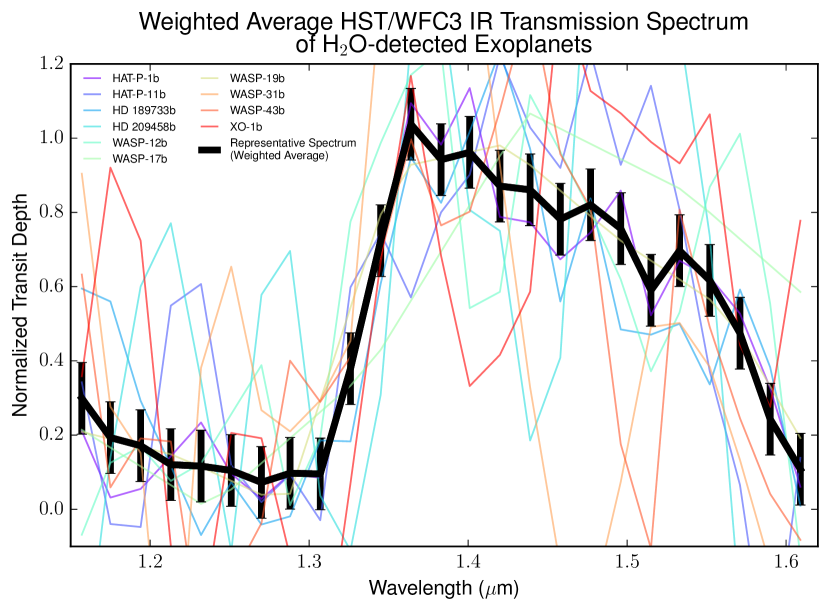
Figure 3.— The normalized HST/WFC3 IR transmission spectra of the 10 exoplanets with reported H₂O-detections (thin lines) are combined with a weighted mean to create a representative spectrum of H₂O-bearing exoplanets (thick black line).

3. Results and Analysis

To test the validity of this H₂O-detected “representative” spectrum, and to understand the emerging patterns pertaining to this group, we compare it with four single-planet clear (cloud and haze-free) atmosphere models with H₂O abundances of 0.1, 1, 10, and 100 ppm. We include Rayleigh scattering and H₂/H₂ and H₂/He collisionally induced absorption as additional opacity sources in these models, as the planets in our sample are predominantly hot Jupiters with hydrogen and helium atmospheres. These models are also normalized between 0 and 1 to facilitate the comparison of their shape to that of the representative spectrum (Fig. 4, Top). We find that the amplitude of the representative spectrum is consistent with H₂O abundances of 10 to 100 ppm.

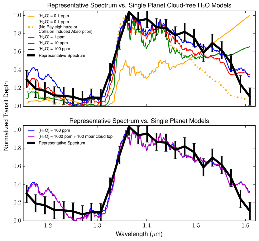
Figure 4.— Single planet models with Rayleigh haze slope of 1 (computed using Equation 1 of Lecavelier Des Etangs et al., 2008) with the CHIMERA routine (Line et al., 2013a; Swain et al., 2014; Kreidberg et al., 2014b, 2015) and assuming H₂/H₂ and H₂/He collisionally induced absorption in addition to the following: Top: Cloud-free forward models of varying H₂O abundances (thin multi-color lines) compared to the representative spectrum (thick black line, see Fig. 3). The increase in transit depth at longer wavelengths for the [H₂O] = 0.1 ppm model is due to H₂/H₂ and H₂/He collisionally induced absorption. We illustrate this effect with an [H₂O] = 0.1 ppm model without these opacity sources (yellow dashed line). Higher H₂O abundance models have enough H₂O to mask these features, yielding a similar spectral shape when normalized. Bottom: Two forward models, one cloud-free with [H₂O] = 100 ppm (thin blue line) and the other with [H₂O] = 1000 ppm and a cloud top at 100 mbar (thin purple line), are compared to the representative spectrum (thick black line). These two models are nearly identical and as such fit the representative spectrum similarly well, illustrating the degeneracy of the cloud-top pressure and the water abundance.

Additionally, we also explore the effect of clouds on the H₂O spectral modulation amplitude to explain the shape of the representative spectrum. We compare the representative spectrum to a forward model with [H₂O] = 1000 ppm and a cloud top at 100 mbar, alongside a cloud-free model with [H₂O] = 100 ppm (Fig. 4, Bottom). The choice of H₂O mixing ratio and cloud-top pressure were selected to match best to the representative spectrum. Both models show a good qualitative fit relative to the representative spectrum indicating a degeneracy between the cloud-free and cloudy solutions.

To explore the range of values for the water mixing ratio that are consistent with the data, we perform a $\Delta\chi^{2}$ search of the parameter space by computing forward models and comparing their shape with the representative spectrum (Fig. 5, left). To generate these forward models, we use parameters of a ‘representative planet’ by computing the average T_eq, R_p, R_s and log(g) of all the water hosting planets in our sample. Cloud-free models with cloud-top pressure of $\geq$1 bar, where they do not interact with the transmission spectrum can be consistent with the data. Larger values for the H₂O mixing ratio can also be consistent with the data, but are degenerate with cloud-top pressure (Benneke, 2015; Kreidberg et al., 2015). However, we can estimate the degree to which clouds block portions of the atmosphere that would otherwise be sampled in a transmission spectrum. Using the representative spectrum’s best-fit cloud-free water abundance of 17 ${}^{+12}_{-6}$ ppm (Fig. 5, left), we compute the spectral modulation for all the planets in our sample in the following way. We run 1000 Monte-Carlo iterations per planet to generate cloud free forward models with [H₂O] abundance sampled from the asymmetrical distribution (Fig. 5, left). Planet parameters of T_eq, R_p, R_s and log(g) unique to each planet are used in the CHIMERA radiative transfer code (Line et al., 2013a; Swain et al., 2014; Kreidberg et al., 2014b, 2015). We then calculate the theoretical cloud-free H₂O spectral modulation derived from the MC for each planet, which is plotted against the measured spectral modulation (Fig. 5, right). By averaging the results for the water-detected planets, we find that clouds likely remove at least half, and possibly more, of the observable atmospheric modulation from participating in a transit measurement.

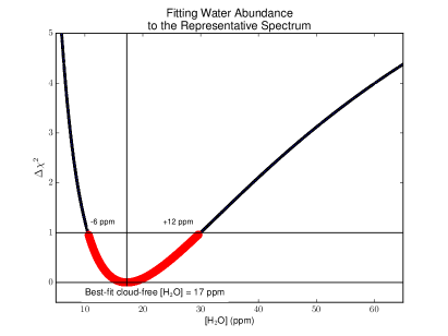
Figure 5.— Left: 10,000 synthetic cloud-free spectra are generated with H₂O abundances between 1 and 1000 ppm. Each spectrum is normalized between 0 and 1 and compared to the representative spectrum (Fig. 3) with a $\Delta\chi^{2}$ calculation. The best fit $\Delta\chi^{2}$ between the synthetic data and the representative spectrum has a [H₂O] = 17 ${}^{+12}_{-6}$ ppm. Right: Clouds typically prevent at least half the potentially measurable atmospheric annulus from being sampled in a transit measurement. We illustrate this by computing the spectral modulation for a cloud free atmosphere using an [H₂O] abundance of 17 ${}^{+12}_{-6}$ ppm. Cloud-free forward models are generated for each HST/WFC3 planet and the observed H₂O spectral modulation is plotted versus the theoretical pure-H₂O modulation derived from the forward models. As a whole, the H₂O-detection reported planets (blue squares) have a mean observed modulation of 1.8$\pm 0.5$ H_s (Fig. 2) compared to a theoretical modulation of 3.20${}^{+0.27}_{-0.30}$ H_s. The ratio of these values represents a maximum value ($\sim$2 H_s) of potentially view-able atmospheric column sampled by the transmission spectrum.

4. Discussions

The H₂O spectral modulation of the HST/WFC3 H₂O-detected exoplanets spans 0.9 to 2.9 $H_{s}$ with a mean modulation of 1.8 $\pm$ 0.5 $H_{s}$. This mean value differs significantly from expectations for the cloud-free H₂O spectral modulation as compared with idealized models which predict $\sim$7 scale heights of spectral modulation (Seager & Sasselov, 2000; Brown, 2001). This reduced H₂O modulation implies the presence of some additional opacity source, such as clouds or aerosol haze, to reduce the true spectral modulation due to H₂O. Aerosol haze has been reported in the atmosphere of the H₂O-hosting hot Jupiter HD 189733b (Lecavelier Des Etangs et al., 2008; Pont et al., 2008; Sing et al., 2009) and clouds have been discussed by Brown (2001) and Morley et al. (2012). Quite literally, we are likely seeing the effects of H₂O above the haze/clouds which are opaque for transit viewing geometry, but may not be so for vertical paths observed during eclipse. This hypothesis agrees with recent findings for some of the planets in our sample by Benneke (2015), Kreidberg et al. (2015) and Sing et al. (2016).

The presence of a cloud deck as a common feature of the hot Jupiter H₂O-hosting planets has implications for recent work which found a measurable difference ($\sim$100$\times$) in the H₂O mixing ratio for the dayside and terminator regions of HD 189733b (Line et al., 2014; Madhusudhan et al., 2014). The spectral modulation due to H₂O in the terminator region is 2.0 $\pm$ 0.5 $H_{s}$. In a scenario where terminator-region clouds are ubiquitous, the dayside measurement can be understood as probing a region in which dayside perpendicular viewing potentially samples 1.3 $H_{s}$ of additional atmospheric path in deeper, higher-pressure regions of the atmosphere. This geometry allows for more H₂O opacity to be present in the emission spectrum and a correspondingly large value is determined for the H₂O mixing ratio.

5. Conclusions

Although we now possess the observational evidence to support the conclusion that H₂O is a common constituent of the atmospheres of hot Jupiter exoplanets, much of the water these atmospheres contain may be hidden beneath clouds. When the spectral modulation due to H₂O is measured in units of the atmospheric scale height, we find that the average H₂O-induced modulation is 1.8 $\pm$ 0.5 $H_{s}$ and never exceeds 2.9 $H_{s}$. The shape of the spectral modulation is also inconsistent with extremely low H₂O abundances and suggests that a cloud layer may obscure a significant portion of the otherwise observable atmosphere. We also find that the sample of H₂O-hosting planets possesses a representative spectral shape dominated by opacity due to H₂O. The fact that the individual spectra coherently average to a consistent shape for the H₂O-hosting planets, which is reproducible with simple forward models, gives confidence that there is a representative spectrum for at least a significant portion of the hot Jupiter exoplanet population.

6. Acknowledgements

We are grateful to Dr. Yan Betremieux, Dr. David Crisp, Dr. Wladimir Lyra, and Dr. Yuk L. Yung for several insightful discussions on our analysis and suggestions for edits on the paper draft.

This research is based on observations made with the NASA/ESA Hubble Space Telescope, obtained from the Data Archive at the Space Telescope Science Institute, which is operated by the Association of Universities for Research in Astronomy, Inc., under NASA contract NAS 5-26555.

We thank the JPL Exoplanet Science Initiative for partial support of this work. The research was carried out at the Jet Propulsion Laboratory, California Institute of Technology, under a contract with the National Aeronautics and Space Administration. $\copyright$ 2015. All rights reserved.

This research has made use of the Exoplanet Orbit Database and the Exoplanet Data Explorer at exoplanets.org.

We thank the anonymous referee for their helpful comments.

References

- Barman (2008) Barman, T. S. 2008, ApJ, 676, L61
- Benneke (2015) Benneke, B. 2015, ArXiv e-prints
- Brown (2001) Brown, T. M. 2001, ApJ, 553, 1006
- Deming et al. (2013) Deming, D., Wilkins, A., McCullough, P., Burrows, A., Fortney, J. J., Agol, E., Dobbs-Dixon, I., Madhusudhan, N., Crouzet, N., Desert, J.-M., Gilliland, R. L., Haynes, K., Knutson, H. A., Line, M., Magic, Z., Mandell, A. M., Ranjan, S., Charbonneau, D., Clampin, M., Seager, S., & Showman, A. P. 2013, ApJ, 774, 95
- Ehrenreich et al. (2014) Ehrenreich, D., Bonfils, X., Lovis, C., Delfosse, X., Forveille, T., Mayor, M., Neves, V., Santos, N. C., Udry, S., & Ségransan, D. 2014, A&A, 570, A89
- Fraine et al. (2014) Fraine, J., Deming, D., Benneke, B., Knutson, H., Jordán, A., Espinoza, N., Madhusudhan, N., Wilkins, A., & Todorov, K. 2014, Nature, 513, 526
- Grillmair et al. (2008) Grillmair, C. J., Burrows, A., Charbonneau, D., Armus, L., Stauffer, J., Meadows, V., van Cleve, J., von Braun, K., & Levine, D. 2008, Nature, 456, 767
- Han et al. (2014) Han, E., Wang, S. X., Wright, J. T., Feng, Y. K., Zhao, M., Fakhouri, O., Brown, J. I., & Hancock, C. 2014, PASP, 126, 827
- Huitson et al. (2013) Huitson, C. M., Sing, D. K., Pont, F., Fortney, J. J., Burrows, A. S., Wilson, P. A., Ballester, G. E., Nikolov, N., Gibson, N. P., Deming, D., Aigrain, S., Evans, T. M., Henry, G. W., Lecavelier des Etangs, A., Showman, A. P., Vidal-Madjar, A., & Zahnle, K. 2013, MNRAS, 434, 3252
- Knutson et al. (2014a) Knutson, H. A., Benneke, B., Deming, D., & Homeier, D. 2014a, Nature, 505, 66
- Knutson et al. (2014b) Knutson, H. A., Dragomir, D., Kreidberg, L., Kempton, E. M.-R., McCullough, P. R., Fortney, J. J., Bean, J. L., Gillon, M., Homeier, D., & Howard, A. W. 2014b, ApJ, 794, 155
- Kreidberg et al. (2014a) Kreidberg, L., Bean, J. L., Désert, J.-M., Benneke, B., Deming, D., Stevenson, K. B., Seager, S., Berta-Thompson, Z., Seifahrt, A., & Homeier, D. 2014a, Nature, 505, 69
- Kreidberg et al. (2014b) Kreidberg, L., Bean, J. L., Désert, J.-M., Line, M. R., Fortney, J. J., Madhusudhan, N., Stevenson, K. B., Showman, A. P., Charbonneau, D., McCullough, P. R., Seager, S., Burrows, A., Henry, G. W., Williamson, M., Kataria, T., & Homeier, D. 2014b, ApJ, 793, L27
- Kreidberg et al. (2015) Kreidberg, L., Line, M. R., Bean, J. L., Stevenson, K. B., Desert, J.-M., Madhusudhan, N., Fortney, J. J., Barstow, J. K., Henry, G. W., Williamson, M., & Showman, A. P. 2015, ArXiv e-prints
- Lecavelier Des Etangs et al. (2008) Lecavelier Des Etangs, A., Pont, F., Vidal-Madjar, A., & Sing, D. 2008, A&A, 481, L83
- Line et al. (2013b) Line, M. R., Knutson, H., Deming, D., Wilkins, A., & Desert, J.-M. 2013b, ApJ, 778, 183
- Line et al. (2014) Line, M. R., Knutson, H., Wolf, A. S., & Yung, Y. L. 2014, ApJ, 783, 70
- Line et al. (2013a) Line, M. R., Wolf, A. S., Zhang, X., Knutson, H., Kammer, J. A., Ellison, E., Deroo, P., Crisp, D., & Yung, Y. L. 2013a, ApJ, 775, 137
- Madhusudhan et al. (2014) Madhusudhan, N., Crouzet, N., McCullough, P. R., Deming, D., & Hedges, C. 2014, ApJ, 791, L9
- Mandell et al. (2013) Mandell, A. M., Haynes, K., Sinukoff, E., Madhusudhan, N., Burrows, A., & Deming, D. 2013, ApJ, 779, 128
- Markwardt (2009) Markwardt, C. B. 2009, in Astronomical Society of the Pacific Conference Series, Vol. 411, Astronomical Data Analysis Software and Systems XVIII, ed. D. A. Bohlender, D. Durand, & P. Dowler, 251
- McCullough et al. (2014) McCullough, P. R., Crouzet, N., Deming, D., & Madhusudhan, N. 2014, ApJ, 791, 55
- Mendez (2014) Mendez, A. 2014, in Habitable Worlds Across Time and Space, proceedings of a conference held April 28-May 1 2014 at the Space Telescope Science Institute. Online at href=”http://www.stsci.edu/institute/conference/habitable-worlds”, id.32, 32
- Morley et al. (2012) Morley, C. V., Fortney, J. J., Marley, M. S., Visscher, C., Saumon, D., & Leggett, S. K. 2012, ApJ, 756, 172
- Pont et al. (2008) Pont, F., Knutson, H., Gilliland, R. L., Moutou, C., & Charbonneau, D. 2008, MNRAS, 385, 109
- Ranjan et al. (2014) Ranjan, S., Charbonneau, D., Désert, J.-M., Madhusudhan, N., Deming, D., Wilkins, A., & Mandell, A. M. 2014, ApJ, 785, 148
- Schwartz & Cowan (2015) Schwartz, J. C., & Cowan, N. B. 2015, MNRAS, 449, 4192
- Seager & Sasselov (2000) Seager, S., & Sasselov, D. D. 2000, ApJ, 537, 916
- Sing et al. (2009) Sing, D. K., Désert, J.-M., Lecavelier Des Etangs, A., Ballester, G. E., Vidal-Madjar, A., Parmentier, V., Hebrard, G., & Henry, G. W. 2009, A&A, 505, 891
- Sing et al. (2016) Sing, D. K., Fortney, J. J., Nikolov, N., Wakeford, H. R., Kataria, T., Evans, T. M., Aigrain, S., Ballester, G. E., Burrows, A. S., Deming, D., Désert, J.-M., Gibson, N. P., Henry, G. W., Huitson, C. M., Knutson, H. A., Etangs, A. L. d., Pont, F., Showman, A. P., Vidal-Madjar, A., Williamson, M. H., & Wilson, P. A. 2016, Nature, 529, 59
- Sing et al. (2015) Sing, D. K., Wakeford, H. R., Showman, A. P., Nikolov, N., Fortney, J. J., Burrows, A. S., Ballester, G. E., Deming, D., Aigrain, S., Désert, J.-M., Gibson, N. P., Henry, G. W., Knutson, H., Lecavelier des Etangs, A., Pont, F., Vidal-Madjar, A., Williamson, M. W., & Wilson, P. A. 2015, MNRAS, 446, 2428
- Swain et al. (2014) Swain, M. R., Line, M. R., & Deroo, P. 2014, ApJ, 784, 133
- Swain et al. (2008) Swain, M. R., Vasisht, G., & Tinetti, G. 2008, Nature, 452, 329
- Tinetti et al. (2007) Tinetti, G., Vidal-Madjar, A., Liang, M.-C., Beaulieu, J.-P., Yung, Y., Carey, S., Barber, R. J., Tennyson, J., Ribas, I., Allard, N., Ballester, G. E., Sing, D. K., & Selsis, F. 2007, Nature, 448, 169
- Wakeford et al. (2013) Wakeford, H. R., Sing, D. K., Deming, D., Gibson, N. P., Fortney, J. J., Burrows, A. S., Ballester, G., Nikolov, N., Aigrain, S., Henry, G., Knutson, H., Lecavelier des Etangs, A., Pont, F., Showman, A. P., Vidal-Madjar, A., & Zahnle, K. 2013, MNRAS, 435, 3481
- Wilkins et al. (2014) Wilkins, A. N., Deming, D., Madhusudhan, N., Burrows, A., Knutson, H., McCullough, P., & Ranjan, S. 2014, ApJ, 783, 113