Smoothed Dissipative Particle Dynamics model for mesoscopic multiphase flows in the presence of thermal fluctuations

Abstract

Thermal fluctuations cause perturbations of fluid-fluid interfaces and highly nonlinear hydrodynamics in multiphase flows. In this work, we develop a novel multiphase smoothed dissipative particle dynamics model. This model accounts for both bulk hydrodynamics and interfacial fluctuations. Interfacial surface tension is modeled by imposing a pairwise force between SDPD particles. We show that the relationship between the model parameters and surface tension, previously derived under the assumption of zero thermal fluctuation, is accurate for fluid systems at low temperature but overestimates the surface tension for intermediate and large thermal fluctuations. To analyze the effect of thermal fluctuations on surface tension, we construct a coarse-grained Euler lattice model based on the mean field theory and derive a semi-analytical formula to directly relate the surface tension to model parameters for a wide range of temperatures and model resolutions. We demonstrate that the present method correctly models the dynamic processes, such as bubble coalescence and capillary spectra across the interface.

I Introduction

Thermal fluctuations originating from molecular interactions can profoundly affect the behavior of multiphase fluid systems, resulting in emergent phenomena reflected on the hydrodynamic length scale. Consistent coupling of the molecular and hydrodynamic scales is at the heart of mesoscale framework development. At the fluid-fluid interface, capillary waves generated by thermal fluctuations result in stochastic and highly nonlinear interfacial dynamics Ortiz de Zárate et al. (2004). This dynamics plays an important role in many physical and biological processes, such as spreading of nano droplets Davidovitch et al. (2005), breakup of nano-jets Moseler and Landman (2000), Rayleigh-Taylor instabilities Kadau et al. (2007), and protein mobility within membranes Quemeneur et al. (2014). Numerical modeling of such processes must accurately account for fluid momentum transport in bulk and interfacial dynamics under thermal fluctuations.

Traditionally, thermally driven mesoscale flows are described by so-called fluctuating hydrodynamics (FHD) (also known as Landau-Lifshitz-Navier-Stokes (LLNS)) equations Landau and Lifshitz (1987). These equations extend the hydrodynamic Navier-Stokes (NS) description by adding spatiotemporal delta-function-correlated random stress in the NS equations with the stress covariance determined from the fluctuation-dissipation theorem. Several numerical methods have been developed to solve LLNS equations, including finite difference Atzberger et al. (2007); Atzberger (2011); Voulgarakis and Chu (2009), finite volume Serrano and Español (2001); Bell et al. (2007); Donev et al. (2010, 2011), and Lattice-Boltzmann methods Ladd (1993). Extending these grid-based methods to mesoscale multiphase and/or multicomponent flows requires coupling FHD with additional thermodynamic equations or appropriate boundary conditions at the interface between two fluids Español and Thieulot (2003); Shang et al. (2011). Specifically, the interface between two fluids yields the FHD equations highly nonlinear, and it is nontrivial to numerically solve them with grid-based methods. Recently, grid-based methods have been used to solve coupled LLNS-free energy equations to model multiphase mesoscale flows (i.e., liquid and gas phases of the same fluid). For example, Shang et al. Shang et al. (2011) solved the FHD equations coupled with the Ginzburg-Landau free energy model by using a heuristic correction for the observed unphysical negative density fluctuations across the interface. Donev et al. Chaudhri et al. (2014) solved the FHD equations coupled with a free energy model based on van der Waals equations. In this work, the surface tension is imposed through Korteweg stress, which requires further parameter calibration and can be sensitive to spatial discretization.

In this paper, we present a rescaled Pairwise-Force Smoothed Dissipative Particle Dynamics (rPF-SDPD) method for mesoscale multicomponent flows. The rPF-SDPD model combines the Pairwise-Force Smoothed Particle Hydrodynamics (PF-SPH) method for multiphase multicomponent flows in the absence of thermal fluctuations Tartakovsky and Meakin (2005a); Tartakovsky and Panchenko (2015) with the Smoothed Dissipative Particle Dynamics (SDPD) Español and Revenga (2003); Grmela and Öttinger (1997); Öttinger and Grmela (1997) method. The major difference between PF-SPH and the present rPF-SDPD model is that rPF-SDPD accounts for the effect of interfacial thermal fluctuations on the interfacial surface tension and, therefore, can be used to study mesoscale multicomponent flows. The SDPD model can be derived from the Smoothed Particle Hydrodynamics method (SPH) Gingold and Monaghan (1977); Lucy (1977); Monaghan (2005) by adding random forces, satisfying the fluctuation-dissipation theorem. Both SPH and SDPD are fully Lagrangian particle methods. In both methods, the fluid domain is discretized with a set of points (also refereed to as fluid particles). Due to their Lagrangian nature, the SDPD and SPH methods are well suited for multicomponent flow simulations because they do not require any interface tracking schemes to evolve the interface between different fluid components. In these methods, each fluid is represented by its own set of particles with positions advected by fluid velocities.

The SPH method has been extensively used for multicomponent and multiphase simulations. There are two main SPH approaches for imposing surface tension at fluid-fluid interfaces that can be extended to SDPD. The first approach is based on the Continuum Surface Force (CSF) method Brackbill et al. (1992); Hu and Adams (2006) and requires estimating the local normal vectors and curvatures at the interface by means of a color function Morris (2000); Hu and Adams (2006, 2009). Accurate estimation of these variables requires sufficient resolution at the interface, i.e., the radii of the largest curvature corresponding to interfacial roughness should be much larger than the SPH smoothing parameter $h$, which plays the same role as grid size in grid-based methods. It has been demonstrated that the CSF-SDPD method yields accurate results for macroscopic multiphase flows where thermally induced interface oscillations are not pronounced Hu and Adams (2006). For problems with large front oscillations, the effect of interfacial roughness on the CSF-SDPD accuracy requires additional investigations.

The second approach is the PF-SPH method, where pairwise molecular-like forces are added into the SPH momentum conservation equation to produce surface tension at the fluid-fluid interface Tartakovsky and Meakin (2005a); Tartakovsky and Panchenko (2015). Unlike the CSF-based SPH method, the PF-SPH method does not require estimates of the normal and curvature of the interface.

In this paper, we focus on moderate thermal fluctuations and their effects on the oscillations of the interface between fluids. Starting with the PF-SPH method, developed for low-temperature smooth interfaces (radii of curvature much greater than $h$), we analyze the effect of thermal-fluctuation-induced interface roughness by constructing a coarse-grained lattice model based on a mean field theory. The coarse-grained model enables us to extract a universal scaling relationship between surface tension and the thermal fluctuations for various model resolutions (i.e., $h$) and construct a semi-analytical relationship between the surface tension and model parameters. We demonstrate that the numerical values of the surface tension imposed by the proposed method agree well with the theoretical predictions based on the correct rescaled formulation. We also show that the structure factor of the perturbed interface correctly scales with the wave number.

In this work, we distinguish between macroscopic (in the absence of thermal fluctuations) and mesoscopic (in the presence of fluctuations) surface tensions and use the following notation:

• $\sigma$ – mesoscopic surface tension across a nearly flat interface with local roughness induced by fluctuations due to the thermal energy $k_{B}T$

• $\sigma_{0}$ – macroscopic surface tension across flat and smooth interface (without local roughness)

• $\tilde{\sigma}(R,k_{B}T)$ – mesoscopic surface tension across the interface with curvature radii R and local roughness induced by fluctuations due to the thermal energy $k_{B}T$

• $\sigma^{N}$ – numerical value of surface tension obtained from a direct simulation

• $\sigma^{F}$ – surface tension obtained from numerical fitting to the scaling relationship.

The paper is organized as follows. Section II introduces the governing equations of the multiphase flow and their discrete SDPD counterparts. In Section III, we show that the “zero-thermal fluctuations” relationship between the surface tension and force parameters overestimates the surface tension of mesoscale fluids in the presence of thermal fluctuations. To accurately account for the effect of thermal fluctuations, we introduce a coarse-grained lattice model based on the mean field theory. We establish a semi-analytical relationship between the temperature-dependent surface tension and model parameters through proper scaling among different model resolutions. In Section IV, we demonstrate that the present method yields consistent thermodynamic properties and further show that the present method captures the correct dynamic processes in multiphase flow, such as bubble coalescence dynamics and capillary wave spectra of an interface with and without external gravity field. Conclusions are given in Section V.

II Numerical model

II.1 Governing equations

We consider the flow of $\alpha$ and $\beta$ fluid components, occupying the domains $\Omega_{\alpha}(t)$ and $\Omega_{\beta}(t)$, respectively, with a sharp boundary $\Gamma(t)=\Omega_{\alpha}(t)\cap\Omega_{\beta}(t)$ separating the two fluids. We assume that at the mesoscale, flow of these fluids can be described by the isothermal stochastic Navier-Stokes equations Ortiz de Zárate et al. (2004), including the continuity equation

$$\frac{D\rho_{l}}{Dt}=-{\rho_{l}}\left({\bm{\nabla}\cdot\bm{v}}_{l}\right),\quad\mathbf{x}\in\Omega_{l},\quad l=\alpha,\beta$$ (1)

and the momentum conservation equation

$$\frac{D\bm{v}_{l}}{Dt}=-\frac{1}{\rho_{l}}\bm{\nabla}P_{l}+\frac{1}{\rho_{l}}\bm{\nabla}\cdot\bm{\tau}_{l}+\bm{g}+\frac{1}{\rho_{l}}\bm{\nabla}\cdot\bm{s}_{l},\quad\mathbf{x}\in\Omega_{l},\quad l=\alpha,\beta.$$ (2)

Here $D/Dt=\partial/\partial t+\bm{v}_{l}\cdot\bm{\nabla}$ is the total derivative; $\rho_{l}$, $\bm{v}_{l}$, and $P_{l}$ are the density, velocity, and pressure; and $\bm{g}$ is the body force. The components of the viscous stress $\bm{\tau}_{l}$ are given by

$$\tau^{ik}_{l}= \mu_{l}\left(\frac{\partial v^{i}_{l}}{\partial x^{k}}+\frac{\partial v^{k}_{l}}{\partial x^{i}}\right),$$ (3)

where $\mu_{l}$ is the (shear) viscosity ($l=\alpha,\beta$) and the bulk viscosity of the $l$-fluid component is assumed to be equal to $\frac{2}{3}\mu_{l}$.

Fluctuations in velocity are caused by the random stress tensor

$$\bm{s}_{l}=\gamma_{l}\bm{\xi},$$ (4)

where $\bm{\xi}$ is a random symmetric tensor (which components are random Gaussian variables), and $\gamma_{l}$ is the strength of the noise. The random stress is related to the viscous stress by the fluctuation-dissipation theorem Landau and Lifshitz (1987). For incompressible and low-compressible fluids, the covariance of the stress components is:

$$\overline{{s^{in}_{l}(\mathbf{x}_{1},t_{1})s^{jm}(\mathbf{x}_{2},t_{2})}}=\gamma^{2}_{l}\delta(\mathbf{x}_{1}-\mathbf{x}_{2})\delta(t_{1}-t_{2})\hskip 14.22636pt\gamma^{2}_{l}=2\mu_{l}k_{B}T\delta^{ij}\delta^{nm},$$ (5)

where $k_{B}$ is the Boltzmann constant, $T$ denotes the temperature, $\delta(z)$ is the Dirac delta function, and $\delta^{ij}$ is the Kronecker delta function.

For generality, we treat the fluids as compressible and prescribe an equation of state $P_{l}=f(\rho_{l})$ for each phase to close Eqs. (1) and (2). Eqs. (1) and (2) are subject to the no-slip boundary conditions for the fluid velocity at the fluid-solid boundary

$$v_{l,n}=0\hskip 14.22636pt\text{and}\hskip 14.22636ptv_{l,\tau}=0,\quad l=\alpha,\beta,$$ (6)

and the dynamic Young-Laplace boundary condition for pressure and velocity at the fluid-fluid-interface

$$(P_{\alpha}-P_{\beta})\mathbf{n}=(\bm{\tau}_{\alpha}-\bm{\tau}_{\beta})\cdot\mathbf{n}+\kappa\sigma\mathbf{n},\quad\mathbf{x}\in\Gamma,$$ (7)

where $v_{l,n}$ and $v_{l,\tau}$ are the normal and tangent components of velocity; $\kappa$ is the curvature of the interface; and $\sigma$ is the surface tension between $\alpha$ and $\beta$ fluids. The normal vector $\bf n$ is pointed away from the non-wetting phase. In this work, we are interested in the dynamics of fluid-fluid interfaces, so we will only consider cases not involving fluid-fluid-solid interfaces. Otherwise, the contact angle at the fluid-fluid-solid interface would also need to be prescribed. Eqs. (1) and (2) are subject to the initial conditions

$$\mathbf{v}_{l}(\mathbf{x},t=0)=\mathbf{v}_{l}^{0}(\mathbf{x}),\quad\Omega_{l}(t=0)=\Omega^{0}_{l},\quad\rho_{l}(\mathbf{x},t)=\rho_{l}^{0},\quad l=\alpha,\beta.$$ (8)

II.2 Smoothed Dissipative Particle Hydrodynamics

In the SDPD method, the computational domains $\Omega_{\alpha}$ and $\Omega_{\beta}$ are discretized with $N_{\alpha}$ and $N_{\beta}$ points (usually referred to as particles) with initial positions $\mathbf{r}_{i}^{0}$. It is convenient, but not necessary, to initially put particles on a Cartesian mesh with grid size $\Delta$ discretizing the domain $\Omega=\Omega_{\alpha}\cup\Omega_{\beta}$. The particles within domains $\Omega_{\alpha}^{0}$ and $\Omega_{\beta}^{0}$ can then be labeled as $\alpha$ and $\beta$ particles, respectively, and the particles are assigned the viscosities of the corresponding fluids. The mass of particle $i$ in domain $\Omega_{l}$ is set to $m_{i}=\rho^{0}_{l}\Delta^{d}$, and the initial particle density of particle $i$ is $n_{i}^{0}=n_{eq}=\Delta^{-d}$, where $d$ is the number of spatial dimensions. Eq. (2) is approximated as

$$\frac{D\mathbf{r}_{i}}{Dt}=\mathbf{v}_{i},\quad m_{i}\frac{D\mathbf{v}_{i}}{Dt}=\sum_{j=1}^{N}\left(\mathbf{F}_{ij}^{P}+\mathbf{F}^{visc}_{ij}+\mathbf{F}_{ij}^{S}\right)+\mathbf{F}_{i}^{b},$$ (9)

where $N=N_{\alpha}+N_{\beta}$ and the summation is over all particles,

$$\mathbf{F}_{ij}^{P}=-\left(\frac{P_{j}}{n_{j}^{2}}+\frac{P_{i}}{n_{i}^{2}}\right)\frac{\mathbf{r}_{ij}}{r_{ij}}\frac{dW(r_{ij},h)}{dr_{ij}},$$ (10)

$$\mathbf{F}^{visc}_{ij}=\frac{5(\mu_{i}+\mu_{j})}{6n_{i}n_{j}}\frac{1}{r_{ij}}\frac{dW(r_{ij},h)}{dr_{ij}}\left[\mathbf{v}_{ij}+\left(\mathbf{v}_{ij}\cdot\frac{\mathbf{r}_{ij}}{r_{ij}}\right)\frac{\mathbf{r}_{ij}}{r_{ij}}\right],$$ (11)

and $\mathbf{F}_{ij}^{S}$ is

$$\mathbf{F}_{ij}^{S}=B_{ij}\frac{\mathbf{r}_{ij}}{r_{ij}}d\tilde{\bm{\mathcal{W}}}_{ij},$$ (12)

where ${\bf r}_{ij}={\bf r}_{i}-{\bf r}_{j}$ and $r_{ij}=|{\bf r}_{ij}|$. In Eq. (12),

$$B_{ij}=\sqrt{-\frac{20}{6}k_{B}T\frac{(\mu_{i}+\mu_{j})}{n_{i}n_{j}}\frac{1}{r_{ij}}\frac{dW(r_{ij},h)}{dr_{ij}}},$$ (13)

$d\tilde{\bm{\mathcal{W}}}_{ij}=(d\bm{\mathcal{W}}_{ij}+\bm{\mathcal{W}}_{ij}^{T})$, and $\bm{\mathcal{W}}_{ij}$ is the matrix of independent increments of the Wiener process.

The random number $\tilde{\zeta}^{l}_{ij}=\tilde{\zeta}^{l}_{ji}$ has a Gaussian distribution with zero mean and unit variance, and superscript $l$ denotes $l$-component of vectors. $\mathbf{F}_{i}^{b}$ is the body (e.g., gravitational) force acting on particle $i$. In the preceding expressions, $W$ is the ”smoothed” Dirac delta function with compact support $h$, which integrates to one, and in the limit of $h\to 0$ approaches the Dirac delta function. In this work, we use $W$ in the form of the fourth-order spline function Morris (1997):

$$W(r,h)=\frac{81}{359\pi h^{3}}\left\{\begin{array}[]{l l r l l}\left(3-\frac{3|\bm{r}|}{h}\right)^{5}-6\left(2-\frac{3|\bm{r}|}{h}\right)^{5}+15\left(1-\frac{3|\bm{r}|}{h}\right)^{5}&&0\leq|\bm{r}|&<\frac{1}{3}&h\\ \left(3-\frac{3|\bm{r}|}{h}\right)^{5}-6\left(2-\frac{3|\bm{r}|}{h}\right)^{5}&&\frac{1}{3}h\leq|\bm{r}|&<\frac{2}{3}&h\\ \left(3-\frac{3|\bm{r}|}{h}\right)^{5}&&\frac{2}{3}h\leq|\bm{r}|&<&h\\ 0&&|\bm{r}|&>&h\end{array}\right.$$ (18)

In Eq. (9), $\sum_{j=1}^{N}{F}_{ij}^{P}$ and $\sum_{j=1}^{N}\mathbf{F}^{visc}_{ij}$ terms are obtained using the SPH discretization of the $\nabla P$ and $\mu\nabla^{2}\mathbf{v}$ terms in the NS equation, respectively. The $\mathbf{F}_{ij}^{S}$ force is derived from the expression (11) of the viscous/dissipative force using the fluctuation-dissipation theorem instead of directly discretizing the $\nabla\cdot\mathbf{s}$ term in Eq. (2). The number density $n_{i}=\rho_{i}/m_{i}$ can be computed by integrating an ordinary differential equation (ODE) obtained from the SPH discretization of the continuity equation (1), but it is more common in SDPD to compute density as

$$n_{i}=\sum_{j}W(r_{ij},h).$$ (19)

In this work, we use the equation of state

$$P=\frac{c^{2}\rho_{0}}{7}\left[\left(\frac{\rho}{\rho_{0}}\right)^{7}-1\right],$$ (20)

where $c$ is the speed of sound and $\rho_{0}$ is the equilibrium density.

II.3 Pairwise-Force Smoothed Dissipative Particle Hydrodynamics for low-temperature multicomponent flows

To impose the boundary condition (7), we add the pairwise interaction forces

$${\bf{F}}_{ij}^{int}={\bf{F}}^{int}(\mathbf{r}_{ij})=-s_{ij}\phi(r_{ij})\frac{\mathbf{r}_{ij}}{r_{ij}}$$ (21)

into the momentum equation,

$$m_{i}\frac{D\mathbf{v}_{i}}{Dt}=\sum_{j=1}^{N}\left(\mathbf{F}_{ij}^{P}+\mathbf{F}^{visc}_{ij}+\mathbf{F}_{ij}^{S}+\mathbf{F}^{int}_{ij}\right)+\mathbf{F}_{i}^{b},$$ (22)

where $\phi(r_{ij})$ is the so-called shape factor, to be defined later, and

$$s_{ij}=\left\{{\begin{array}[]{*{20}{c}}s_{\alpha\beta},&\;\mathbf{r}_{i}\in\Omega_{\alpha}\quad\text{and}\quad\mathbf{r}_{j}\in\Omega_{\beta},\\ s_{\alpha\alpha},&\;\mathbf{r}_{i}\in\Omega_{\alpha}\quad\text{and}\quad\mathbf{r}_{j}\in\Omega_{\alpha},\\ s_{\beta\beta},&\;\mathbf{r}_{i}\in\Omega_{\beta}\quad\text{and}\quad\mathbf{r}_{j}\in\Omega_{\beta}.\\ \end{array}}\right.$$ (23)

The force ${\bf{F}}_{ij}^{int}$ is a molecular-like pairwise interaction force acting between particle $i$ of the $\alpha$ phase and particle $j$ of the $\beta$ phase. The shape function $\phi$ is selected such that ${\bf{F}}_{ij}^{int}$ behaves as a pairwise molecular force, i.e., ${\bf{F}}_{ij}^{int}$ is short-range repulsive ($F_{\alpha,\beta}(r_{ij}\leq r^{*})<0$, $r^{*}<h$) and long-range attractive ($F_{\alpha,\beta}(r^{*}<r_{ij}\leq h)>0$). For computational efficiency, $\phi$ should be zero (or decay rapidly) for $r_{ij}\geq h$. A similar approach to impose the boundary conditions (7) has been used in an SPH multiphase flow model Tartakovsky and Meakin (2005a, b); Tartakovsky et al. (2009); Gouet-Kaplan et al. (2009); Kordilla et al. (2013); Tartakovsky and Panchenko (2015).

Various forms of $\phi$ have been proposed in literature, and it has been shown that $\phi$ affects particle distribution. Here, we use

$$\phi=r_{ij}\left[-Ae^{-\frac{r_{ij}^{2}}{2{r_{a}}^{2}}}+e^{-\frac{r_{ij}^{2}}{2{r_{b}}^{2}}}\right],$$ (24)

where $r_{a}=r_{b}/2=\Delta/2$, which we found to result in a relatively uniform particle distribution for a given surface tension value.

It has been demonstrated that, in the absence of thermal fluctuations (i.e., for $\mathbf{F}_{ij}^{S}=0$), the parameters in ${\bf{F}}_{ij}^{int}$ can be related to the “macroscopic” surface tension $\sigma_{0}$ as

$$s_{\alpha\alpha}=s_{\beta\beta}=10^{k}s_{\alpha\beta}=\frac{1}{2(1-10^{-k})}n^{-2}_{eq}\frac{\sigma_{0}}{\lambda},$$ (25)

where $k>1$ and

$$\lambda=\frac{\pi}{8}\int\limits_{0}^{\infty}z^{4}\phi(z)dz=\pi(-A\varepsilon_{0}^{6}+\varepsilon^{6}).$$ (26)

The expression (25) is obtained using the Gibbs treatment Rowlinson and Widom (2002), where $\sigma$ is related to the total fluid stress as

$$\sigma(\mathbf{x})=\int_{-\infty}^{+\infty}[T_{\tau}(z)-T_{n}(z)]dz,\quad\mathbf{x}\in\Gamma.$$ (27)

Here, $T_{n}(z)=T_{zz}(z)$ and $T_{\tau}(z)$ are the normal and tangent components of the stress, and the integration is done along the line crossing $\Gamma$ in the normal direction at point $\mathbf{x}$.

The stress $\mathbf{T}$ can be found in terms of the forces acting between SDPD particles according to the Hardy formula (Hardy, 1982):

$${\mathbf{T}}(\mathbf{x})={\mathbf{T}}_{(c)}(\mathbf{x})+{\mathbf{T}}_{(int)}(\mathbf{x}),$$ (28)

where ${\mathbf{T}}_{(c)}(\mathbf{x})$ is the convection stress,

$${\mathbf{T}}_{(c)}(\mathbf{x})=-\sum_{j=1}^{N}m_{j}(\overline{\mathbf{v}}(\mathbf{x})-\mathbf{v}_{j})\otimes(\overline{\mathbf{v}}(\mathbf{x})-\mathbf{v}_{j})\tilde{\psi}_{\eta}(\mathbf{x}-\mathbf{r}_{j}),$$ (29)

and ${\mathbf{T}}_{(int)}(\mathbf{x})$ is the interaction stress,

$$\mathbf{T}_{(int)}(\mathbf{x})=\frac{1}{2}\sum_{i=1}^{N}\sum_{j=1}^{N}\mathbf{f}_{ij}\otimes(\mathbf{r}_{j}-\mathbf{r}_{i})\int_{0}^{1}\tilde{\psi}_{\eta}(\mathbf{x}-s\mathbf{r}_{i}-(1-s)\mathbf{r}_{j})ds,$$ (30)

where $\overline{\mathbf{v}}(\mathbf{x})=\sum_{j}m_{j}\mathbf{v}_{j}\tilde{\psi}_{\eta}(\mathbf{x}-\mathbf{r}_{j})\left(\sum_{j}m_{j}\tilde{\psi}_{\eta}(\mathbf{x}-\mathbf{r}_{j})\right)^{-1}$ is the average velocity and $\mathbf{f}_{ij}=\mathbf{F}_{ij}^{P}+\mathbf{F}^{visc}_{ij}+\mathbf{F}_{ij}^{S}+\mathbf{F}^{int}_{ij}$ is the total force acting between a pair of $i$ and $j$ particles. The summation here is over all particles, and $\otimes$ denotes a dyadic product of vectors. The weighting function $\tilde{\psi}(\mathbf{x})$ is a “smooth” approximation of the Dirac delta function and can be chosen fairly arbitrary. Here, we assume that $\tilde{\psi}(\mathbf{x})$ is the product of one-dimensional functions $\psi_{\eta,l}=\frac{1}{\eta}\psi\left(\mathbf{x}_{(l)}\right)$, where $l=1,2,3$ denotes a vector component. The function $\psi_{\eta,l}(\mathbf{x})$ has compact support $\eta$, or becomes sufficiently small for $|\mathbf{r}|>\eta$. In our calculations, we set $\eta=h$.

The surface tension between any two fluids only depends on the properties of the two fluids and (weakly depends) on the radii of the interface curvature, but not on the fluid velocities. As shown in Sec. IV.2, the modeled surface tension in our model is independent of curvature smaller than $\frac{1}{2h}$ for a wide range of temperatures. To derive the relationship between ${\bf{F}}_{ij}^{int}$ and $\sigma$, we first assume the two fluids are separated by an interface with the radii of curvature much larger than $\eta$ (and $h$). The dependence of surface tension on large curvatures will be addressed in Section IV.2. Under the assumption of small curvature, the interface can be locally treated as flat. Because the surface tension is independent of flow conditions, without loss of generality, we consider the system at equilibrium. It should be noted that in the presence of thermal fluctuations, SDPD particles move, even at equilibrium. However, in the following derivations, we disregard the mesoscale effects and compute the macroscale surface tension $\sigma_{0}$, i.e., we assume that $\mathbf{F}^{visc}_{ij}+\mathbf{F}_{ij}^{S}$ and $\mathbf{T}_{(c)}$ have zero net contribution to $\sigma_{0}$. Furthermore, it was demonstrated in Tartakovsky and Panchenko (2015) that if the same average particle density is used to discretize both fluid phases, then the $\mathbf{F}_{ij}^{P}$ has exactly zero contribution to the surface tension. Finally, Eq. (27) can be replaced with

$$\sigma_{0}(\mathbf{x})=\int_{-\infty}^{+\infty}[\tilde{T}_{\tau}(z)-\tilde{T}_{n}(z)]dz,\quad\mathbf{x}\in\Gamma$$ (31)

where $\tilde{T}_{n}(z)=\tilde{T}_{zz}(z)$ and $\tilde{T}_{\tau}(z)$ are the normal and tangent components of the stress

$$\tilde{\mathbf{T}}_{(int)}(\mathbf{x})=\frac{1}{2}\sum_{i=1}^{N}\sum_{j=1}^{N}\mathbf{F}_{ij}^{int}\otimes(\mathbf{r}_{j}-\mathbf{r}_{i})\int_{0}^{1}\tilde{\psi}_{\eta}(\mathbf{x}-s\mathbf{r}_{i}-(1-s)\mathbf{r}_{j})ds.$$ (32)

The next step in deriving Eq. (25) and (26) is to approximate Eq. (32) with

$$\tilde{\mathbf{T}}_{(int)}(\mathbf{x})=-\frac{1}{2}n^{2}_{eq}\int_{\Omega}\int_{\Omega}g(\mathbf{r}^{\prime},\mathbf{r}^{\prime\prime})\mathbf{F}^{int}(\mathbf{r}^{\prime}-\mathbf{r}^{\prime\prime})\otimes(\mathbf{r}^{\prime}-\mathbf{r}^{\prime\prime})\int_{0}^{1}\tilde{\psi}_{\eta}(\mathbf{x}-s\mathbf{r}^{\prime}-(1-s)\mathbf{r}^{\prime\prime})dsd\mathbf{r}^{\prime}d\mathbf{r}^{\prime\prime},$$ (33)

where $g(\mathbf{r}^{\prime},\mathbf{r}^{\prime\prime})$ is the pair distribution function Allen and Tildesley (1989). Assuming that

$$g(\mathbf{r}^{\prime},\mathbf{r}^{\prime\prime})=\left\{{\begin{array}[]{*{20}{c}}g_{\alpha\beta}(\left|\mathbf{r}^{\prime}-\mathbf{r}^{\prime\prime}\right|),&\;\mathbf{r}^{\prime}\in\Omega_{\alpha}\quad\text{and}\quad\mathbf{r}^{\prime\prime}\in\Omega_{\beta},\\ g_{\alpha\alpha}(\left|\mathbf{r}^{\prime}-\mathbf{r}^{\prime\prime}\right|),&\;\mathbf{r}^{\prime}\in\Omega_{\alpha}\quad\text{and}\quad\mathbf{r}^{\prime\prime}\in\Omega_{\alpha},\\ g_{\beta\beta}(\left|\mathbf{r}^{\prime}-\mathbf{r}^{\prime\prime}\right|),&\;\mathbf{r}^{\prime}\in\Omega_{\beta}\quad\text{and}\quad\mathbf{r}^{\prime\prime}\in\Omega_{\beta},\\ \end{array}}\right.$$ (34)

substituting Eq. (33) in Eq. (31) and integrating the latter yields

$$\sigma_{0}=s_{\alpha\alpha}\frac{\pi}{8}n_{eq}^{2}\int_{0}^{\infty}g_{\alpha\alpha}(r)\phi(r)r^{4}dr+s_{\beta\beta}\frac{\pi}{8}n_{eq}^{2}\int_{0}^{\infty}g_{\beta\beta}(r)\phi(r)r^{4}dr-2s_{\alpha\beta}\frac{\pi}{8}n_{eq}^{2}\int_{0}^{\infty}g_{\alpha\beta}(r)\phi(r)r^{4}dr.$$ (35)

Eq. (35) is an extension of an expression for the surface tension of a single-component multiphase molecular system (an $\alpha$-liquid in equilibrium with its gas phase) given in Rowlinson and Widom (2002). This expression assumes that molecules are interacting via a pairwise force $s_{\alpha\alpha}\tilde{\phi}(r)$, $s_{\beta\beta}=s_{\alpha\beta}=0$, and $n_{eq}$ is the particle density of the liquid phase. To make expression (35) computable, $g_{kl}(r)$ ($(k,l)=\alpha,\beta$) must be defined. A simple approximation is $g(r)=1$, which is equivalent to treating Eq. (32) as a Riemann sum. This reduces Eq. (33) to an expression obtained by Rayleigh Rayleigh (1964) for a surface tension between two fluids made of molecules interacting via the pairwise force $s_{kl}\tilde{\phi}(r)$ ($(k,l)=\alpha,\beta$). Under the assumption $g(r)=1$, Eqs. (25) and (26) follow directly from Eq. (35). The details of integration in Eq. (35) in two spatial dimensions are given in Tartakovsky and Panchenko (2015), and the extension to the three-dimensional case is straightforward.

Remark II.1

We emphasize that Eqs. (25) and (35) are derived with the assumption that the interface between $\Omega_{\alpha}$ and $\Omega_{\beta}$ is flat, and that these equations should hold for any interface with the radii of the largest curvature much larger than $h$, the range of the SDPD forces. In the next section, we show that Eqs. (25) and (35) accurately describe the relationship between the surface tension and pairwise forces for macroscopic systems (where thermal fluctuations are relatively small or absent) characterized by $\sigma_{0}$. For a mesoscale fluid system, the interfacial roughness, induced by thermal fluctuations, may affect the surface tension $\sigma$. In the following section, we quantify the relationship between $\sigma$, $\sigma_{0}$, $k_{B}T$, and other model parameters.

III Effect of thermal fluctuations: mean field theory analysis and numerical error quantification

In this section, we study temperature dependence of the surface tension for the model introduced in Section II. First, we validate the method by comparing the surface tension from direct simulation with the value prescribed by Eq. (25). Here, we prescribe “low” temperatures (to be rigorously defined in Secton III.4) to keep thermally induced fluctuations small and the fluid interface essentially flat. In this context, the low temperature refers to the macroscopic limit of the SDPD model, where thermal fluctuations are negligible, rather than the absolute low state of thermal energy.

Next, we demonstrate that, for higher temperatures, Eq. (25) overestimates the surface tension by a value further dependent on $n_{eq}$.

To explore the effect of thermal fluctuations on the surface tension, we construct an Euler lattice model based on mean field theory and obtain a universal scaling relationship that accounts for the effect of interfacial roughness for various thermal fluctuations and model resolutions. We then propose a semi-analytical formula to relate the surface tension to model parameters and quantify the numerical error for different temperatures and model resolutions.

III.1 Low temperature

We numerically compute the surface tension between two fluids separated by a nearly flat interface using Eq. (27). We model a layer of one fluid surrounded by two layers of another fluid with $n_{eq}=27$, $46.656$, $64$, and $91.125$. In all of these simulations, the temperature, speed of sound, and surface tension are set to $k_{B}T=0.001$, $c=6.0$, and $\sigma_{0}=2.1$, respectively. The parameters $s_{\alpha\alpha}$, $s_{\beta\beta}$, and $s_{\alpha\beta}$ are found from Eq. (25). The temperature is chosen so the fluid interface remains essentially flat. The simulation domain size is $10\times 10\times 16$ with fluid $\alpha$ placed between $-3<z<3$ and fluid $\beta$ occupying the rest of the domain. The periodic boundary conditions are used in all directions.

Figure 1(a) shows an example of the normal and tangent stresses across the interface for $n_{eq}=27$. Similar computations are conducted for other number densities. For each combination of parameters, $10$ independent simulations are performed, and $T_{\tau}$ and $T_{n}$ are computed using the simulation data from the last $10000$ time steps. Figure 1(b) shows the relative numerical error, $\varepsilon=|1-\sigma^{N}/\sigma_{0}|$, for different $n_{eq}$. Here, $\sigma^{N}$ is the surface tension obtained from direct simulations using Eq. (27). As $n_{eq}$ increases from $27$ to $64$, $\varepsilon$ decreases from $4.7\%$ to $2.4\%$, respectively. However, $\varepsilon$ does not further decrease as $n_{eq}$ increases from 64 to $91.125$. One possible reason for this plateau result is the uniform distribution assumption, $g(r)\equiv 1$, in the derivation of Eq. (25), which is not fully satisfied even for large $n_{eq}$. Nevertheless, for all considered $n_{eq}$, the error is less than $5\%$.

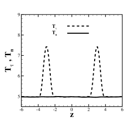
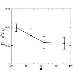
Figure 1: (a) Normal and tangential hardy stress $T_{n}$ and $T_{\tau}$ computed across the interface of the two-phase fluid layer located at $z=-3.0$ and $z=3.0$. (b) Numerical error of imposed surface tension versus $n_{eq}$ at $k_{B}T=0.001$.

III.2 Effect of thermal fluctuations

In this section, we model the multiphase system, described in Section III.1, with different temperatures. Figure 2 shows the computed surface tension for different $n_{eq}$, with $k_{B}T$ between $0$ and $0.06$. As $k_{B}T$ increases, the interfacial roughness gets more pronounced (also see Sec. IV.4), and the surface tension decreases accordingly. Eq. (25) accurately predicts the surface tension at the low temperature, but it overestimates the surface tension at higher temperatures. Moreover, we observe that the simulated surface tension values, obtained at different $k_{B}T$, further depend on $n_{eq}$. Given the same value at the low-temperature limit, the surface tension exhibits different temperature-dependent behaviors for different $n_{eq}$. For low resolutions (e.g., $n_{eq}=27$), the surface tension shows weak dependence on $T$, while for high resolutions, the surface tension decreases more rapidly as $T$ increases. To model multiphase flow with thermal fluctuations, we need to understand the relationship between $\sigma$ and $\sigma_{0}$, $k_{B}T$, and $n_{eq}$.

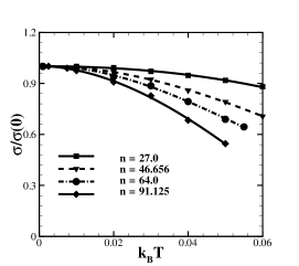
Figure 2: Surface tension between the two-phase flow computed at different temperatures.

III.3 Coarse-grained lattice model

To quantify the effect of thermal fluctuation on the surface tension, we coarse grain the system by replacing the present Lagrangian particle system with a Euler lattice, similar to the work of Widom (1984); Rowlinson and Widom (2002); Dawson (1987). Figure 3 shows a sketch of the mapping process. For each model resolution with $n_{eq}=\Delta^{-3}$ (in three spacial dimensions), we map the system on the lattice with the lattice size $\Delta$. For each lattice unit, we define the number density of each lattice $(i,j,k)$ as $n^{L}_{ijk}$. Given a flat interface, $n^{L}=1$ within the $\alpha$ fluid region and $0$, otherwise.

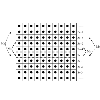
Figure 3: A sketch of the coarse-grained lattice model, where the Lagrangian-based particle model is mapped into a discrete lattice. The lattice layer $z_{0}$ (e.g., the one between the horizontal dashed lines) interacts with the neighboring layers $z_{0}\pm 1$, $z_{0}\pm 2$, $\ldots$, $z_{0}\pm L$ with interaction energy $M_{1}$, $M_{2}$, $\ldots$, $M_{L}$, respectively.

For each lattice unit, we assume the energy can be approximated by a mean field, i.e., $u^{L}=\epsilon n^{L}$, where $\epsilon$ is the potential energy of the lattice filled with an SDPD particle

$$\epsilon=\int_{0}^{\infty}4\pi u(r)g(r)r^{2}dr\approx\int_{0}^{\infty}4\pi u(r)r^{2}dr,$$ (36)

where $u(r)$ is the potential energy between two fluid particles due to the interaction force, $du(r)/dr=s_{\alpha\alpha}\phi(r)$. Similar to Ref. Rowlinson and Widom (2002), we define the activity $\zeta(n^{L},k_{B}T)$ for each lattice unit, such that the probability to fill the lattice with an SDPD particle is

$$n^{L}/\zeta=(1-n^{L})e^{-u^{L}/k_{B}T}.$$ (37)

Therefore, the activity of each lattice unit is given by

$$\zeta(n^{L},k_{B}T)=\frac{n^{L}}{1-n^{L}}e^{\epsilon n^{L}/k_{B}T}.$$ (38)

Under equilibrium conditions, the equilibrium activity $\zeta$ satisfies the equal area rule Rowlinson and Widom (2002)

$$\int_{n^{L}_{g}}^{n^{L}_{l}}\ln\left[\frac{\zeta(n^{\prime},k_{B}T)}{\zeta}\right]dn^{\prime}=0,~{}~{}\zeta(n^{L}_{g})=\zeta(n^{L}_{l})$$ (39)

where $n^{L}_{g}$ and $n^{L}_{l}$ are the nontrivial solutions ($\neq 0.5$) corresponding to the coexisting densities of the gas and liquid phases. This gives the equilibrium activity $\zeta$ by

$$\zeta=e^{\epsilon/2k_{B}T}.$$ (40)

Next, we consider the inhomogeneous fluid system. Without loss of generality, we assume the interface is normal to $z$ direction and denote the lattice number density as $n^{L}(z)$. As shown in Figure 3, the lattice unit at layer $z_{0}$ interacts with the neighboring layers $z_{0}-L,z_{0}-L+1,\ldots,z_{0},\ldots,z_{0}+L-1,z_{0}+L$, where $L$ is determined by the cut-off distance of pairwise force interaction $h$ and lattice unit length $\Delta$ by

$$L=\left\lceil\frac{h}{\Delta}\right\rceil.$$ (41)

The energy $u^{L}(z_{0})$ of a lattice unit at layer $z_{0}$ is determined by the interaction energy with the neighboring layers, which is given by

$$\begin{split}&u^{L}(z_{0})=\epsilon n^{L}(z_{0})+\sum_{l=1}^{L}M_{l}\Delta_{l}^{2}n^{L}(z_{0})\\ &\Delta_{l}^{2}n^{L}(z_{0})=n^{L}(z_{0}+l)+n^{L}(z_{0}-l)-2n^{L}(z_{0}),\end{split}$$ (42)

where $\epsilon n^{L}(z_{0})$ represents the energy of the lattice unit under homogeneous assumption, $M_{l}$ represents the interaction energy between two layers of homogeneous fluid with distance $l\Delta$, and $M_{l}(n^{L}(z_{0}+l)-n^{L}(z_{0}))$ represents the change of potential energy if the number density of the $(z_{0}+l)th$ layer is changed from homogeneous assumption to $n^{L}(z_{0}+l)$.

$M_{l}$ is related to the forces acting between SDPD particles, including ${\bf{F}}_{ij}^{int}$, and can be determined in an iterative manner. As shown in Figure 3, we first consider the interaction between layer $z_{0}$ and $z_{0}+L$. For a single particle in layer $z_{0}+L$ with distance $z$ to the upper layer $z_{0}$, the attractive force is

$$\psi(z)=\int_{z}^{\infty}2\pi z^{\prime}n_{eq}u(z)dz^{\prime}.$$ (43)

Therefore, the total interaction force between layers $z_{0}$ and $z_{0}+l$ is

$$\theta(z)=\int_{(L-1)\Delta}^{\infty}\psi(z^{\prime})n_{eq}dz^{\prime},$$ (44)

and the interaction energy $M_{L}$ between layers $z_{0}$ and $z_{0}+L$ is

$$W_{L}=\int_{(L-1)\Delta}^{\infty}\theta(z^{\prime})dz^{\prime},M_{L}=W_{L}.$$ (45)

Next, we consider the interaction energy $W_{L-1}$ between the layers $\left[z_{0}-1,z_{0}\right]$ and $\left[z_{0}+L-1,z_{0}+L\right]$. We note that the interaction energy between layer $z_{0}$ and $z_{0}+L$, as well as layer $z_{0}-1$ and $z_{0}+L-1$, is $M_{L}$. Analysis, similar to Eqs. (44) and (45), gives

$$W_{L-1}=\int_{(L-2)\Delta}^{\infty}\theta(z^{\prime})dz^{\prime},~{}~{}2M_{L}+M_{L-1}=W_{L-1}.$$ (46)

Repeating the preceding process, $M_{l}$ can be obtained as

$$\begin{split}\sum_{k=l}^{L}(k-l+1)M_{k}=W_{l}\\ W_{l}=\int_{(l-1)\Delta}^{\infty}\theta(z^{\prime})dz^{\prime},\end{split}$$ (47)

where $M_{l+1},\ldots,M_{L}$ are found iteratively.

Combining Eqs. (36), (40), and (47), we can rewrite Eq. (37) as Widom (1984)

$$\begin{split}&-\sum_{l=1}^{L}M_{l}\Delta_{l}^{2}n^{L}(z)=F^{\prime}\left[n^{L}(z)\right],\\ &F^{\prime}\left[n^{L}(z)\right]=-\epsilon\left(\frac{1}{2}-n^{L}(z)\right)+k_{B}T\ln\left[n^{L}/(1-n^{L})\right].\end{split}$$ (48)

This is the governing equation for the inhomogeneous density $n^{L}(z)$ of the coarse-grained lattice model, with asymptotic solutions $n^{L}(-\infty)=n^{L}_{g}$ and $n^{L}(\infty)=n^{L}_{l}$ satisfying

$$F^{\prime}(n^{L}_{g})=F^{\prime}(n^{L}_{l})=0.$$ (49)

By solving Eq. (48), we can explore the intrinsic relationship between the Lagrangian particle model and the coarse-grained lattice model, as well as quantify the effect of the thermal fluctuations of the surface tension for different $n_{eq}$, as discussed in Section III.4.

III.4 Effect of thermal fluctuations: scaling and error analysis

The numerical solution of Eq. (48) is complicated by a stiff nonlinear term $k_{B}T\ln\left[n^{L}/(1-n^{L})\right]$. To simplify the problem, we introduce the change of variables

$$n^{L}(z)=\frac{e^{x(z)}}{1+e^{x(z)}},$$ (50)

rewrite Eq. (48) as

$$\begin{split}&-\sum_{l=1}^{L}M_{l}\delta_{l}^{2}{x(z)}=-\epsilon\left(\frac{1}{2}-\frac{e^{x(z)}}{1+e^{x(z)}}\right)+k_{B}T{x(z)},\\ &\delta_{l}^{2}{x(z)}=\frac{e^{x(z+l)}}{1+e^{x(z+l)}}+\frac{e^{x(z-l)}}{1+e^{x(z-l)}}-\frac{2e^{x(z)}}{1+e^{x(z)}},\end{split}$$ (51)

and solve it using the Newton-Raphson method on the discrete lattice plane at $z=\ldots,-3/2,-1/2,1/2,3/2,\ldots$. The surface tension of the lattice model can be determined as

$$\begin{split}\sigma=\sum_{z=-\infty}^{\infty}\left\{F\left[n^{L}(z)\right]+\frac{1}{2}\sum_{l=1}^{L}M_{l}\left[\Delta_{l}n^{L}(z)\right]^{2}\right\}\\ \Delta_{l}n^{L}(z)=n^{L}(z+l)-n^{L}(z),~{}~{}F(n)=\int_{n^{L}_{g}}^{n^{L}_{l}}F^{\prime}(n)dn.\end{split}$$ (52)

To explore the effect of thermal fluctuations on the modeled surface tension, we map the Lagrangian SDPD particles with different $n_{eq}$ on a discrete lattice following the procedure introduced in Section III.3. For each $n_{eq}$, we choose $\sigma=2.1$ at $k_{B}T=0.001$ similar to Section III.1 and solve Eq. (48) numerically with $\epsilon$ and $M_{l}$ obtained from Eqs. (36) and (47), respectively.

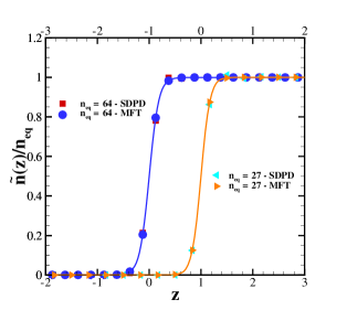
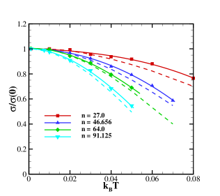
Figure 4: (a) Normalized interfacial density profile $\tilde{n}(z)$ obtained from both the direct SDPD simulation and the mean field theory from Eq. (48) at $k_{B}T=0.03$. For the SDPD model, $\tilde{n}(z)$ is defined as the number density of the SDPD particle with the binning size as $\Delta$ along the $z$ direction. (b) Temperature-dependent surface tension obtained from the direct simulation and the present lattice model. $\sigma(0)$ represents the numerical value of the surface tension at $k_{B}T=0.001$.

Figure 4(a) compares the density profiles obtained from the the direct simulations and the lattice model with $n_{eq}=27$ and 64 and $k_{B}T=0.03$. In the lattice model, we numerically solve Eq. (51) with $\epsilon$ and $M_{l}$, obtained from Eqs. (36) and (47), respectively. Good agreement is achieved for both $n_{eq}=27$ and $n_{eq}=64$. Figure 4(b) shows the surface tensions obtained from the SDPD lattice models for different $k_{B}T$ values. It can be seen that the lattice model successfully captures the modeled surface tension’s dependence on $k_{B}T$ and $n_{eq}$. The difference in $\sigma$ obtained from the lattice model and SDPD is mainly due to the mean field approximation of the energy in Eqs. (36) and (42). As $n_{eq}$ increases, the agreement between the two models improves. This result not only validates the intrinsic relationship between the present method and the coarse-grained lattice model, established through Eqs. (36), (47), and (42), but also indicates that the lattice model is a convenient tool for studying the effect of thermal fluctuations on the surface tension in the present model.

Inspired by the lattice model, we revisit Eq. (39). It is possible to define the transition temperature

$$-\epsilon^{L}/(k_{B}T_{c})^{L}=4,$$ (53)

above which only the trivial solution exists. Here, the superscript “$L$” represents the unit lattice length scale $\Delta$. With $k_{B}T=k_{B}T_{c}^{L}$, Eq. (39) only has the trivial solution $n^{L}_{g}=n^{L}_{l}=0.5$, and the surface tension decays to $0$.

We compute $\epsilon$ from Eq. (36) for different $n_{eq}$ and represent the results in the lattice model units. Because $\epsilon$ and $k_{B}T$ scale with length unit $\left[L\right]$ as $\epsilon\sim\left[L\right]^{5}$ and $k_{B}T\sim\left[L\right]^{2}$, where $\left[L\right]$ represents the length unit of the lattice model, we have

$$-\frac{\epsilon/(\Delta)^{5}}{k_{B}T_{c}/(\Delta)^{2}}=4.$$ (54)

For $n_{eq}=27$, $46.656$, $64$, and $91.125$, the predicted transition temperature $k_{B}T_{c}$ is $0.198$, $0.135$, $0.108$, and $0.087$, respectively.

These results indicate that although the particle model of different spatial resolution yields the same surface tension when $k_{B}T$ approaches zero, the transition temperature of the corresponding lattice model is different, leading to different temperature-dependent surface tensions for large $k_{B}T$. Another way to understand this is to note that the SDPD fluid of different $n_{eq}$ modeled by Eq. (25) yields the same interaction energy (i.e., $\sum_{l=1}^{L}lM_{l}$) and, therefore, the same surface tension between neighboring layers. However, the total energy $\epsilon^{L}$ varies for different $n_{eq}$, leading to a dependence of $\sigma$ on $n_{eq}$. In particular, smaller $n_{eq}$ yields larger $\epsilon^{L}$, leading to a smaller response to interfacial fluctuations. Therefore, $\sigma$ decays more slowly for low $n_{eq}$ when $k_{B}T$ increases.

Based on the preceding analysis, we propose a scaling relationship that relates the surface tension to the model parameters for different $n_{eq}$, i.e.,

$$\sigma(k_{B}T,n_{eq},\epsilon)=f\left(\frac{k_{B}T}{n_{eq}\epsilon}\right),$$ (55)

where $\epsilon$ is determined by Eq. (36) and the functional form of $f$ depends on the form of $\mathbf{F}^{int}_{ij}$.

Eq. (55) is the main theoretical result of this study. It suggests that the imposed surface tension at $k_{B}T$, $\sigma(k_{B}T)$ can be related to the parameters of the rPF-SDPD model, including $k_{B}T$, $n_{eq}$, and surface tension at the “macroscopic” interface with zero thermal fluctuations, $\sigma_{0}$, through a unified scaling relationship. For the $\mathbf{F}^{int}_{ij}$ given by Eq. (24) and used in this study, we propose an approximate form for $f$

$$\sigma^{F}(k_{B}T,n_{eq},\epsilon)=\sigma_{0}\left(1-b\left(\frac{k_{B}T}{n_{eq}\epsilon}\right)^{2}\right)^{2},$$ (56)

where $b=12.4$ is a fitting parameter.

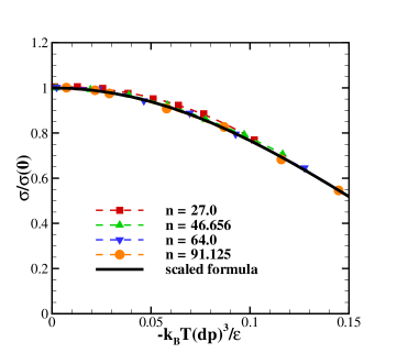
Figure 5: Surface tension with respect to $-\frac{k_{B}T\Delta^{3}}{\epsilon}$ obtained from the direct simulation and Eq. (56). $\sigma(0)$ represents the numerical value of the surface tension at $k_{B}T=0.001$.

Figure 5 shows the surface tension values $\sigma$ obtained from the rPF-SDPD model and the scaling formula Eq. (56) as a function of $\frac{k_{B}T\Delta^{3}}{\epsilon}$. The simulation results agree well with the scaling formula for all considered $n_{eq}$, with agreement improving with increasing $n_{eq}$.

Table 1 shows the relative differences $\varepsilon=\left|1-\sigma^{N}(k_{B}T)/\sigma^{F}(k_{B}T)\right|$, where $\sigma^{N}$ and $\sigma^{F}$ are the surface tension values obtained from direct simulation of rPF-SDPD and fitting to scaling relationship Eq. (55) through Eq. (56), respectively. For all cases, $\varepsilon$ is less than $5.7\%$ and decreases with increasing $n_{eq}$. This shows that Eq. (56) accurately describes the relationship between the surface tension and $\mathbf{F}^{int}_{ij}$, $n_{eq}$, and $k_{B}T$. In the next section, we demonstrate the accuracy and capabilities of rPF-SDPD by applying it to several mesoscale multicomponent systems.

$n$	$k_{B}T=0.001$	$k_{B}T=0.01$	$k_{B}T=0.02$	$k_{B}T=0.03$	$k_{B}T=0.04$	$k_{B}T=0.05$	$\left<\varepsilon\right>$
$27.0$	$3.80\%$	$4.23\%$	$4.71\%$	$4.57\%$	$4.96\%$	$5.64\%$	$4.88\%$
$46.656$	$3.02\%$	$3.19\%$	$3.57\%$	$3.68\%$	$3.40\%$	$4.67\%$	$3.61\%$
$64.0$	$2.15\%$	$2.75\%$	$1.45\%$	$2.44\%$	$1.63\%$	$1.47\%$	$2.17\%$
$91.125$	$2.09\%$	$1.98\%$	$1.47\%$	$0.80\%$	$2.59\%$	$3.17\%$	$1.49\%$

Table 1: Relative error $\varepsilon=\left|1-\sigma^{N}(k_{B}T)/\sigma^{F}(k_{B}T)\right|$ between the direct simulated surface tension $\sigma^{N}(k_{B}T)$ and the prediction $\sigma^{F}(k_{B}T)$ from the scaling relation Eq. (55) and Eq. (56). $\left<\varepsilon\right>$ represents the average relative error for the different $k_{B}T$ presented here.

Remark III.1

In the lattice model, we use the transition temperature $T_{c}$ to construct a scaling relationship, but we do not simulate the regime of large thermal fluctuations near $T_{c}$. In practice, we note that for $-\frac{k_{B}T\Delta^{3}}{\epsilon}>0.18$, SDPD particles of one fluid phase begin escaping into the fluid region of the other phase, i.e., the interface between the fluids diffuses, which is outside of the present study’s scope. In this work, we consider mesoscale immiscible multicomponent flow, i.e., the flow with a fluctuating but clearly defined interface.

Remark III.2

The scaling expression (56) provides an accurate approximation of direct simulation results as demonstrated in Table 1. However, it is not necessarily a unique expression. Other formulas in terms of $\frac{k_{B}T\Delta^{3}}{\epsilon}$ may be obtained.

Remark III.3

In the present study, we assume the interface has a radius of curvature much larger than $h$ and can be locally approximated as flat. For an interface with a smaller radii of curvature, the surface tension may also depend on the local curvature. We will address this issue in the next section.

IV Numerical examples

Here, we study the accuracy of the rPF-SDPD model. First, we show that rPF-SDPD yields consistent thermodynamic properties for bulk flow with thermal fluctuation. Next, we simulate a droplet of one fluid surrounded by another fluid and quantify the curvature dependence of the modeled surface tension. Finally, we study the dynamics of bubble coalescence and fluctuations of the fluid interface with and without gravity.

IV.1 Thermodynamic properties

We first demonstrate that the present model accurately captures the thermodynamic properties of a bulk fluid, i.e., that in the presence of the pairwise forces $\mathbf{F}_{ij}^{int}$, the probability density function (PDF) of the $x$, $y$, and $z$ velocity components are in good agreement with the Maxwell-Boltzmann distribution,

$$f_{v}(v_{k})=\left(\frac{m}{2\pi k_{B}T}\right)^{\frac{3}{2}}\exp\left(-\frac{mv_{k}^{2}}{2k_{B}T}\right)\quad k=x,y,z,$$ (57)

and the local density fluctuations satisfy

$$\frac{\delta n(d)}{\langle n(d)\rangle}=\sqrt{\frac{k_{B}T}{\langle n(d)\rangle c^{2}d^{3}}},$$ (58)

where $\delta n(d)$ and $\langle n(d)\rangle$ are the standard deviation of density and average density within a cubic domain $\Omega_{d}$ with the edge size $d$, $d^{3}$ is the volume of $\Omega_{d}$, and $c$ is the speed of sound of the bulk fluid.

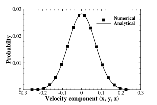
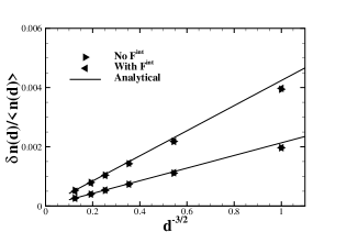
Figure 6: Testing of the mesoscopic method: (a) Probability distribution of the velocity components of an individual mesoscopic particle with $k_{B}T=0.005$. (b) Fluid density fluctuations within different volumes with $k_{B}T=0.005$ and $k_{B}T=0.02$.

We simulate a single-component fluid in a three-dimensional $30\times 30\times 30h^{3}$ box in the absence of gravity. The simulations are initialized by placing particles on a Cartesian mesh with the grid size $\Delta=0.25h$. The initial particle velocity is set to zero, and the fluid density is set to $n_{eq}=64h^{-3}$. The pairwise forces are chosen to be the same as the numerical example presented in Section III.1. At each time step, we compute the PDFs of the velocity components and local density $n(d)$ as

$$n(d)=\frac{\sum_{i}n_{i}\mathrm{I}_{i\in\Omega_{d}}}{\sum_{i}\mathrm{I}_{i\in\Omega_{d}}},$$ (59)

where $\mathrm{I}_{i\in\Omega_{d}}$ is an indicator function equal to $1$ if particle $i$ is inside domain $\Omega_{d}$ and $0$ otherwise; and $n_{i}$, is found from Eq. (19).

Simulations with and without $\mathbf{F}^{int}$ are performed. Figures 6(a) and 6(b) show that $f_{v}(v_{k})$ ($k=x,y,z$) and $\delta n(d)/\langle n(d)\rangle$, obtained from the simulations with and without $\mathbf{F}^{int}$, agree well with the theoretical results given by Eqs. (57) and (58), respectively.

For $d=h$, $\delta n(d)/\langle n(d)\rangle$ is about $6\%$ smaller than the theoretical prediction from Eq. (58). This difference arises because $n_{i}$ in Eq. (59) is defined as a smoothed density with a smoothing length $h$. Therefore, for a small volume $\Omega_{d}$ with $d$ comparable to $h$, the effective volume is a bit larger than $d^{3}$, leading to an underestimation of density fluctuations. Nevertheless, a good agreement is achieved for $d>1.6h$. These results demonstrate that rPF-SDPD yields consistent thermodynamic properties for the nearly incompressible fluids considered in this study.

IV.2 Effect of interfacial curvature: surface tension of a droplet

In this section, we compute the surface tension of a three-dimensional droplet of fluid $\alpha$ immersed in fluid $\beta$. Previous studies show that on the molecular scale, surface tension depends on the curvature of the interface for the radius of curvature comparable with the molecular size (e.g., see Ref. Kashchiev (2003).) Since the interaction forces in rPF-SDPD are similar to molecular forces, it is natural to expect the surface tension in rPF-SDPD to depend on the curvature for the radius of the curvature comparable with the particle size or $h$. In the following, we denote the surface tension of the droplet of radius $R$ as $\tilde{\sigma}(R,k_{B}T)$ and explore the dependence of $\tilde{\sigma}$ on $R$ for various temperatures $k_{B}T$ and number densities $n_{eq}$.

First, we simulate droplets with radii $2.5h$, $3.2h$ and $4.0h$, $k_{B}T=0.001$, and $n_{eq}=64.0h^{-3}$. The computational domain is $14\times 14\times 14h^{3}$ with the periodic boundary conditions in the $x$, $y$, and $z$ directions. The droplet is initially placed in the center of the domain. Pairwise-force parameters are chosen so the surface tension corresponding to the flat interface approximation is $\sigma_{0}=2$. We compute the surface tension using two approaches, Eq. (27) and the Young-Laplace equation

$$\Delta P=\frac{2\tilde{\sigma}(R)}{R},$$ (60)

where $\Delta P$ is the difference between the pressure inside and outside of the droplet. Figures 7(a) and 7(b) show $\Delta P$ and the stress components $T_{n}$ and $T_{\tau}$ for the droplet radii greater than $2h$. For all three cases, the numerical values of $\tilde{\sigma}(R)$ agree well with with the theoretical $\sigma$. These results show that for large radii $R$, $\tilde{\sigma}(R,k_{B}T)$ converges to the surface tension between two layers discussed in Section III, i.e., $\tilde{\sigma}(\infty,k_{B}T)=\sigma(k_{B}T)$.

Next, we compute the surface tension of the droplets with radii smaller than $4h$ for $n_{eq}=27$, $46.656$, and $64.0$ at low temperature ($k_{B}T=0.001$). Figure 7(c) depicts the simulation results. For all $n_{eq}$ and $R<2h$, $\sigma(R)$ decreases with decreasing $R$. This behavior is similar to that of the surface tension of nanoscale droplets, which can be approximated by Kashchiev (2003):

$$\tilde{\sigma}(R)=\sigma\left[1-\exp(-R/R_{0})\right],$$ (61)

where $R_{0}$ is a radius with the magnitude on the order of several fluid molecule diameters. In numerical models, including rPF-SDPD, $\tilde{\sigma}(R)$ is affected by the resolution when the radius of the curvature is of the same order as the spacial model resolution. In the present study, $R_{0}$ should be on the order of $h$ or the size of an SDPD particle. In particular, $\tilde{\sigma}(R)$ converges more quickly to $\sigma$ for larger spatial resolution $n_{eq}$, and, for all considered $n_{eq}$, $\tilde{\sigma}(R)$ approaches to $\sigma$ for $R=2.0h$.

We also examine the effect of thermal fluctuations on the curvature dependence of the surface tension. Figure 7(d) shows the size-dependent surface tension of a droplet $\tilde{\sigma}(R,k_{B}T)$ with $n_{eq}=64$ and $k_{B}T=0.001$, $0.03$, and $0.05$ for $\sigma(k_{B}T)=2.0$, $1.85$, and $1.43$. The parameters $s_{\alpha\beta}$ in the pairwise force are found from Eqs. (25) and (56). As $k_{B}T$ increases, $\tilde{\sigma}(R,k_{B}T)$ shows convergence to $\sigma(k_{B}T)$ at a slower rate than observed in Figure 7(c). This result is not unexpected, and can be understood qualitatively as follows: as $k_{B}T$ increases, the instantaneous interface exhibits larger deviation from the equilibrium spherical interface due to larger thermal fluctuations, leading to more pronounced curvature dependence of the surface tension $\tilde{\sigma}(R,k_{B}T)$.

Finally, we perform additional simulations with various $n_{eq}$ and observe that $\tilde{\sigma}(R,k_{B}T)$ converged to $\sigma$ for the radii of curvature $R$ satisfying

$$R\geq 2h+10\left(\frac{k_{B}T}{\sigma(k_{B}T)}\right)^{\frac{1}{2}}.$$ (62)

To simplify the notation, we use $\sigma$ to represent $\tilde{\sigma}$ in the remaining part of the manuscript (if not otherwise specified).

Remark IV.1

We note that Eq. (62) is an empirical criterion to impose the prescribed surface tension $\sigma(k_{B}T)$ for interface with finite curvature. Theoretical analysis of thermal fluctuation effects on $\tilde{\sigma}(R,k_{B}T)$ is out of scope of the present study. The implications of Eq. (62) on numerics will be discussed in Section V.

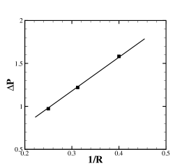
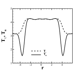
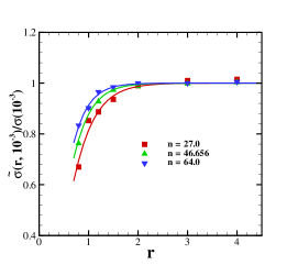
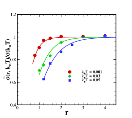
Figure 7: (a) Pressure difference between the inside and outside domain of the droplet of radius $R=2.5$, $3.2$, and $4.0$ with $n_{eq}=64.0$ and $k_{B}T=0.001$. The solid line represents the analytical prediction from the Young-Laplace relationship with $\tilde{\sigma}(R)=\sigma=2.0$. (b) Normal and tangential hardy stress along the radial direction of the droplet of radius $R=4.0$. (c) Surface tension $\tilde{\sigma}(R)$ computed from droplets of different radius $R$ with $k_{B}T=0.001$. The imposed flat interface surface tension $\sigma=2.0$. (d) Surface tension $\tilde{\sigma}(R,k_{B}T)$ computed from droplets of different radius $R$ and $k_{B}T$ with spatial resolution $n=64.0$. The imposed flat interface surface tension is $\sigma(k_{B}T)=2.0$, $1.85$, and $1.43$, respectively.

IV.3 Bubble coalescence

Next, we study the dynamic process of bubble coalescence in a two-phase fluid system similar to Ref. Paulsen et al. (2014). Two bubbles of radius $R=4.0h$ are placed in a simulation domain $24\times 12\times 12h^{3}$ with the centers of the bubbles located at at $[-4.25h,0,0]$ and $[4.25h,0,0]$. The periodic boundary condition is used in the simulations. The spatial resolution $n_{eq}$ and speed of sound $c$ are set to $64.0h^{-3}$ and $6.0$ for both the bubbles ($\alpha$ fluid) and surrounding $\beta$ fluid. The mass density $\rho$ is $0.064$ for $\alpha$ fluid and $64.0$ for $\beta$ fluid. The viscosity $\mu$ is $0.005$ for $\alpha$ fluid and $0.5$ for $\beta$ fluid. As shown in Figure 8(a), we define the instantaneous neck radius $R_{neck}$ of the bubble coalescence region by

$$R_{neck}(t)=\frac{1}{2\pi}\int_{0}^{2\pi}d\theta\int_{0}^{\infty}dr\delta\left(n^{\alpha}(\mathbf{r},t)-\frac{n^{\alpha}_{bulk}}{2}\right),~{}~{}~{}~{}\mathbf{r}=(0,r\cos\theta,r\sin\theta),$$ (63)

where $n^{\alpha}(\mathbf{r},t)$ is the (time-dependent) smoothed number density of fluid $\alpha$ at point $\mathbf{r}$ and $n^{\alpha}_{bulk}$ is the bulk number density of $\alpha$ fluid.

Under such conditions, the rate of bubble coalescence is controlled by the surface tension $\sigma$ between $\alpha$ and $\beta$ fluids  Paulsen et al. (2014):

$$R_{neck}(t)=D_{1}(\sigma R/\rho_{out})^{1/4}t^{1/2}=Kt^{1/2},$$ (64)

where $D_{1}$ is a dimensionless pre-factor, $R$ is the radius of the bubble, and $K$ is the growth rate. We simulate the coalescence process with the surface tension in the range $0.74<\sigma<3.88$. The radius of the largest curvature satisfies Eq. (62) in all of these cases.

Figure 8(b-c) shows the instantaneous neck radius $R_{neck}$ for $k_{B}T=0.003$. The growth rate $K$ depends linearly on $\sigma^{1/4}$, which is consistent with Eq. (64). We also simulate the coalescence process with larger thermal fluctuations corresponding to $k_{B}T=0.03$. In particular, we impose surface tension following two approaches: the low-temperature limit given by Eq. (25) and the thermal fluctuation scaling in Eq. (56). The resulting growth rates are shown in Fig. 8(d). For large surface tensions, both models yield consistent growth rates. However, when $-\frac{k_{B}T\Delta^{3}}{\epsilon}$ is large, Eq. (25) underestimates surface tension and results in slower growth rate. On the other hand, the scaling relation Eq. (56) yields a growth rate consistent with the theoretical result given by Eq. (64) for both $k_{B}T=0.003$ and $k_{B}T=0.03$.

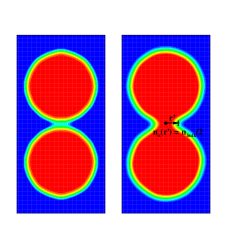
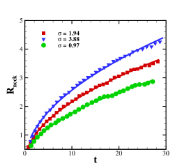
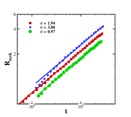
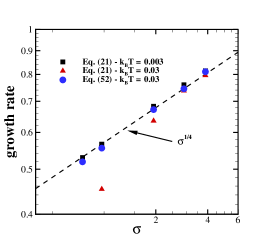
Figure 8: (a) Sketch of the bubble coalescence procedure at initial (left) and intermediate (right) stage. For a specific radial direction $\theta$, $r^{\prime}$ represents the radial distance from center such that $n_{\alpha}(r^{\prime},\theta)=n_{bulk}/2$. (b) The instantaneous neck radius $R_{neck}(t)$ at $k_{B}T=0.003$. (c) $R_{neck}(t)$ plotted in log-log scale. (d) The growth rate measured with different surface tensions and $k_{B}T=0.003$ and $k_{B}T=0.03$.

IV.4 Capillary waves

Finally, we examine the interfacial capillary waves in a two-component fluid system. The entire domain is $[-7,7]\times[-7,7]\times[-10,10]h^{3}$ with fluid $\alpha$ placed between $-5h<z<5h$ and fluid $\beta$ occupying the rest of the domain. The initial particle density is set to $n_{eq}=64h^{-3}$, and the speed of sound is set to $c=6.0$. In the following, we present results at the interface located at $z=5h$. The results for the interface at $z=-5h$ are identical. Because of thermal fluctuations, the interface between fluids $\alpha$ and $\beta$ deviates from a flat plane with the instantaneous height $\eta(x,y)$ defined by

$$n^{\alpha}(x,y,\eta(x,y))=\frac{n^{\alpha}_{bulk}}{2},$$ (65)

where $n^{\alpha}(x,y,z)$ is the smoothed density of phase $\alpha$ at point $(x,y,z)$ and $n^{\alpha}_{bulk}$ is the number density of $\alpha$ fluid in bulk.

For a fluid system in the absence of gravity, the capillary wave theory (CWT) Buff et al. (1965); Evans (1979) predicts that the Fourier modes (a.k.a. the capillary wave spectra) $\hat{\eta}(\mathbf{q})$ of $\eta(x,y)$ are given by

$$\left<\hat{\eta}(\mathbf{q})^{2}\right>=\frac{k_{B}T}{\sigma\left|\mathbf{q}\right|^{2}L^{2}},$$ (66)

where $L\times L$ is the lateral interface domain. With the external gravity field $g$, acting along the $z$ direction, there is an additional potential energy change due to the interface fluctuations, e.g., the work of exchanging the mass density of the lower fluid $\rho_{\alpha}$ to $\rho_{\beta}$. For each $\mathbf{q}$, the contribution to the potential energy difference $\Delta H_{g}$ is given by

$$\Delta H_{g}=\frac{1}{2}\left|\hat{\eta}(\mathbf{q})\right|^{2}(\rho_{\alpha}-\rho_{\beta})gL^{2}.$$ (67)

Therefore, the variance of $\hat{\eta}(\mathbf{q})$ of the fluctuating interface in the presence of gravity $g$ is given by

$$\left<\hat{\eta}(\mathbf{q})^{2}\right>=\frac{k_{B}T}{\sigma\left|\mathbf{q}\right|^{2}L^{2}+(\rho_{\alpha}-\rho_{\beta})gL^{2}}$$ (68)

First, we study the zero-gravity ($g=0$) capillary wave spectra $\hat{\eta}(\mathbf{q})$ with $\rho_{\alpha}=\rho_{\beta}=64.0$ and varying thermal fluctuations. The surface tension $\sigma=2.0$ is imposed, following Eq. (56). Figures 9(a) and 9(b) show $\eta(x,y)$ with $k_{B}T=0.004$, and $0.01$. As expected, $k_{B}T=0.01$ yield larger interfacial fluctuations. Figure 9(c) shows the spectra $\hat{\eta}(\mathbf{q})$ at $k_{B}T=0.004$, $0.01$, $0.03$, and $0.05$. For all $k_{B}T$, $\hat{\eta}(\mathbf{q})$ agrees well with Eq. (66) for low wave numbers and deviates from the CWT prediction for $\left|\mathbf{q}\right|\geq\frac{2\pi}{5h}$, where $h$ is the support of the kernel $W$. This discrepancy is primarily due to the continuum assumption in CWT, where the interfacial energy is modeled as an increased surface area multiplied by the constant surface tension. However, for small length scales, local interfacial energy also depends on the local curvature and interactions between the SDPD particles (also shown in Section IV.2). Therefore, the CWT prediction is not valid for high wave numbers (also see Lei et al. (2015)). Remarkably, for $k_{B}T=0.05$, we also present the spectrum obtained by imposing surface tension directly from Eq. (25); $\left|\hat{\eta}(\mathbf{q})\right|^{2}$ deviates from CWT prediction for all $\mathbf{q}$ due to numerically overestimated interfacial surface tension at high temperatures.

Next, we examine the interfacial fluctuations with a non-zero gravity field and $k_{B}T=0.01$. We consider two cases: (i@) $\rho_{\alpha}=64.0$, $\rho_{\beta}=32.0$, and $g=0.04$. (ii@) $\rho_{\alpha}=32.0$, $\rho_{\beta}=64.0$, and $g=7.5\times 10^{-3}$. Figures. 10(a) and 10(b) show the instantaneous interface $g(x,y)$ for cases (i@) and (ii@), respectively. For case (i@), the lower fluid has larger mass density than the upper fluid. Contributions from the change of gravity potential in Eq. (67) are positive, leading to dampened interfacial fluctuations in Figure 10(a) compared to Figure 9(b). In contrast, in case (ii@), the gravity contribution from Eq. (67) is negative, leading to increased interfacial fluctuations in Figure 10(b) compared to Figure 9(b).

Figure 10(c) shows $\hat{\eta}(\mathbf{q})$ for cases (i@) and (ii@). Numerical results are in good agreement with the predictions from Eq. (68) for $|\mathbf{q}|\leq\frac{2\pi}{5h}$. At high wave numbers, $\hat{\eta}(\mathbf{q})$ deviates from Eq. (68) in a manner similar to the neutral case in Figure 9(c). For case (ii@), we choose $g$ and $\sigma$, satisfying

$$\sigma q_{0}^{2}>(\rho_{\beta}-\rho_{\alpha})g,$$ (69)

where $q_{0}=\frac{2\pi}{L}$ is the lowest wave number such that Rayleigh instability cannot be established. In contrast, if Eq. (69) is violated (e.g., $g=0.014$ and $\sigma=2.0$) Rayleigh instability will be develop as shown in Figure 10(d).

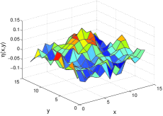
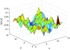
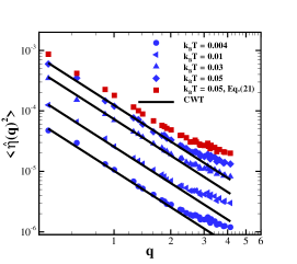
Figure 9: (a) Instantaneous fluid height near the interface at $k_{B}T=0.004$. (b) Instantaneous fluid height near the interface at $k_{B}T=0.01$. (c) The capillary wave spectra measured at different temperatures. For $k_{B}T=0.05$, spectrum with surface tension determined directly from Eq. (25) is also presented.

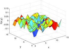
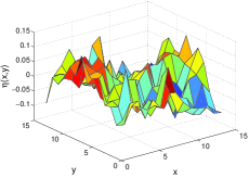
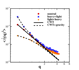
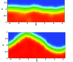
Figure 10: (a) Instantaneous fluid height near the interface with $\rho_{\alpha}=32.0$ and $\rho_{\beta}=64.0$ at $k_{B}T=0.01$. (b) Instantaneous fluid height near the interface with $\rho_{\alpha}=64.0$ and $\rho_{\beta}=32.0$ at $k_{B}T=0.01$. (c) The capillary wave spectra measured at different gravity. (d) Instantaneous density field $n_{\alpha}$ near the fluctuation interface for $g=0.0075$ (upper) and $g=0.014$ (lower). For $g=0.0075$, the two-phase fluid keeps stable fluctuation interface with spectrum shown in (c). For $g=0.014$, Rayleigh instability is established and accompanied by giant fluctuation across the interface.

V Discussion

In this study, we proposed the rescaled Pairwise-Force Smoothed Dissipative Particle Hydrodynamics (rPF-SDPD) method, a fully Lagrangian stochastic particle method designed to model mesoscopic multicomponent immiscible flow with thermal fluctuations. In the rPF-SDPD model, the surface tension between different fluid components is modeled via pairwise interaction forces added to the SDPD momentum conservation equation similar to the PF-SPH model Tartakovsky and Panchenko (2015). In PF-SPH, a relationship between the surface tension and pairwise-force parameters (similar to Eq. (25)) is derived under a locally flat interface assumption. In this work, we demonstrated that, under moderate thermal fluctuations, the modeled surface tension deviates from the analytical result given by Eq. (25) and also depends on the model resolution. To accurately model fluids interfaces, we derived a universal scaling relationship between model parameters (macroscopic surface tension in the absence of thermal fluctuations, temperature, model resolution, and pairwise interaction force) and the surface tension. To establish this relation, we constructed a coarse-grained Euler lattice model by mapping the SDPD particles on a discrete lattice based on a mean field theory. We demonstrated that the numerical results obtained from the present rPF-SDPD model agree well with the theoretical prediction based on the scaling relationship with deviation less than $5\%$.

Furthermore, we demonstrated that the rPF-SDPD model yields consistent thermodynamic properties of the bulk fluid under thermal fluctuations. Moreover, it accurately captures the dynamic processes, such as the bubble coalescence and the capillary wave spectrum under external gravity fields. These results suggest that the present method is wellsuited for a wide application on multiphase immiscible flow on the mesoscopic scale where thermal fluctuations are pronounced, including nanoscale transport processes.

Finally, we observed that for interfaces with radii of curvature less than $2h$, the surface tension decreases with decreasing radii of curvature. Similar results are experimentally observed for real fluids, where the surface tension shows dependence on the radii of curvature for the radii on the order of the molecular size. We note that this length-scale-dependent surface tension (presented in Section IV.2) raises some important issues that require future investigation. In most mesoscopic numerical methods (e.g., see Refs. Hu and Adams (2006, 2009); Chaudhri et al. (2014)) for multiphase and multicomponent flows, the interfacial energy is imposed as the interface area multiplied by a prescribed surface tension coefficient. The implicit assumption therein is that the surface tension is a macroscopic property independent of local interface curvature, i.e., it remains constant as the spatial resolution of the interface increases. This assumption works well for most macroscopic (and many mesoscopic) multiphase flow systems. It also can be achieved for the present method by choosing proper scaling parameters so Eq. (62) is satisfied. However, additional consistency is required when we consider a multiphase flow system on the nanoscale. At this scale, arbitrarily increasing model resolution leads to numerical divergence of interfacial fluctuations, i.e., $\sim\displaystyle{\lim_{{q_{h}}\to\infty}\int_{q_{l}}^{q_{h}}\frac{1}{q^{2}}d^{2}q=\infty}$. On this length scale, surface tension also depends on the local curvature Lum et al. (1999); Huang et al. (2001) with behavior similar to Figure 7. For such systems, accurate fluctuation hydrodynamics modeling requires introduction of molecular fidelity in the form of an effective particle size and local compressibility, as discussed in Ref. Lei et al. (2015). Such use of additional collective variables will be explored in future work.

References

References

- Ortiz de Zárate et al. (2004) J. M. Ortiz de Zárate, F. Peluso, and J. V. Sengers, The European physical journal. E, Soft matter 15, 319 (2004), ISSN 1292-8941.
- Davidovitch et al. (2005) B. Davidovitch, E. Moro, and H. Stone, Physical Review Letters 95, 244505 (2005).
- Moseler and Landman (2000) M. Moseler and U. Landman, Science 289, 1165 (2000).
- Kadau et al. (2007) K. Kadau, C. Rosenblatt, J. L. Barber, T. C. Germann, Z. Huang, P. Carlès, and B. J. Alder, Proceedings of the National Academy of Sciences 104, 7741 (2007).
- Quemeneur et al. (2014) F. Quemeneur, J. K. Sigurdsson, M. Renner, P. J. Atzberger, P. Bassereau, and D. Lacoste, Proceedings of the National Academy of Sciences 111, 5083 (2014).
- Landau and Lifshitz (1987) L. D. Landau and E. M. Lifshitz, Fluid Mechanics: Volume 6 (Course Of Theoretical Physics) (Butterworth-Heinemann, 1987).
- Atzberger et al. (2007) P. J. Atzberger, P. R. Kramer, and C. S. Peskin, Journal of Computational Physics 224, 1255 (2007).
- Atzberger (2011) P. J. Atzberger, Journal of Computational Physics 230, 2821 (2011).
- Voulgarakis and Chu (2009) N. K. Voulgarakis and J.-W. Chu, The Journal of Chemical Physics 130, 134111 (2009).
- Serrano and Español (2001) M. Serrano and P. Español, Phys. Rev. E 64, 046115 (2001).
- Bell et al. (2007) J. B. Bell, A. L. Garcia, and S. A. Williams, Phys. Rev. E 76, 016708 (2007).
- Donev et al. (2010) A. Donev, E. Vanden-Eijnden, A. L. Garcia, and J. B. Bell, Commun. Appl. Math. Comput. Sci. 5, 149 (2010).
- Donev et al. (2011) A. Donev, J. B. Bell, A. de la Fuente, and A. L. Garcia, Phys. Rev. Lett. 106, 204501 (2011).
- Ladd (1993) A. J. C. Ladd, Phys. Rev. Lett. 70, 1339 (1993).
- Español and Thieulot (2003) P. Español and C. Thieulot, The Journal of Chemical Physics 118, 9109 (2003).
- Shang et al. (2011) B. Z. Shang, N. K. Voulgarakis, and J.-W. Chu, The Journal of Chemical Physics 135, 044111 (2011).
- Chaudhri et al. (2014) A. Chaudhri, J. B. Bell, A. L. Garcia, and A. Donev, Physical Review E 90, 033014 (2014).
- Tartakovsky and Meakin (2005a) A. M. Tartakovsky and P. Meakin, Physical Review E 72, 026301 (2005a).
- Tartakovsky and Panchenko (2015) A. Tartakovsky and A. Panchenko, Journal of Computational Physics (2015).
- Español and Revenga (2003) P. Español and M. Revenga, Phys. Rev. E 67, 026705 (2003).
- Grmela and Öttinger (1997) M. Grmela and H. Öttinger, Physical Review E 56, 6620 (1997).
- Öttinger and Grmela (1997) H. Öttinger and M. Grmela, Physical Review E 56, 6633 (1997).
- Gingold and Monaghan (1977) R. A. Gingold and J. J. Monaghan, Mon. Not. R. Astron. Soc. 181, 375 (1977).
- Lucy (1977) L. B. Lucy, Astronomical Journal 82, 1013 (1977).
- Monaghan (2005) J. J. Monaghan, Reports on Progress in Physics 68, 1703 (2005).
- Brackbill et al. (1992) J. Brackbill, D. Kothe, and C. Zemach, Journal of Computational Physics 100, 335 (1992), ISSN 00219991.
- Hu and Adams (2006) X. Y. Hu and N. A. Adams, Journal of Computational Physics 213, 844 (2006).
- Morris (2000) J. P. Morris, International Journal for Numerical Methods in Fluids 33, 333 (2000).
- Hu and Adams (2009) X. Hu and N. Adams, Journal of Computational Physics 228, 2082 (2009).
- Morris (1997) J. P. Morris, Journal of Computational Physics 136, 214 (1997), ISSN 00219991.
- Tartakovsky and Meakin (2005b) A. M. Tartakovsky and P. Meakin, Vadose Zone Journal 4, 848 (2005b), ISSN 1539-1663.
- Tartakovsky et al. (2009) A. M. Tartakovsky, P. Meakin, and A. L. Ward, Transport in Porous Media 76, 11 (2009), ISSN 0169-3913.
- Gouet-Kaplan et al. (2009) M. Gouet-Kaplan, A. M. Tartakovsky, and B. Berkowitz, Water Resources Research 45, 1 (2009), ISSN 0043-1397.
- Kordilla et al. (2013) J. Kordilla, A. M. Tartakovsky, and T. Geyer, Advances in Water Resources 59, 1 (2013), ISSN 03091708.
- Rowlinson and Widom (2002) J. J. S. Rowlinson and B. Widom, Molecular theory of capillarity, vol. 8 (Courier Dover Publications, 2002).
- Hardy (1982) R. J. Hardy, The Journal of Chemical Physics 76, 622 (1982).
- Allen and Tildesley (1989) M. Allen and D. Tildesley, Computer Simulation of Liquids (Clarendon Press, Oxford, 1989), ISBN 0198556454.
- Rayleigh (1964) L. Rayleigh, On the theory of surface forces. In Collected Papers, vol. 3, Art. 176, pp. 397–425 (Dover, New York, 1964).
- Widom (1984) B. Widom, The Journal of Physical Chemistry 88, 6508 (1984).
- Dawson (1987) K. Dawson, Physical Review A 35, 1766 (1987).
- Kashchiev (2003) D. Kashchiev, The Journal of chemical physics 118, 9081 (2003).
- Paulsen et al. (2014) J. D. Paulsen, R. Carmigniani, A. Kannan, J. C. Burton, and S. R. Nagel, Nature Communications 5, 3182 (2014).
- Buff et al. (1965) F. P. Buff, R. A. Lovett, and F. H. Stillinger, Phys. Rev. Lett. 15, 621 (1965).
- Evans (1979) R. Evans, Advances in Physics 28, 143 (1979).
- Lei et al. (2015) H. Lei, C. J. Mundy, G. K. Schenter, and N. K. Voulgarakis, The Journal of Chemical Physics 142, 194504 (2015).
- Lum et al. (1999) K. Lum, D. Chandler, and J. D. Weeks, The Journal of Physical Chemistry B 103, 4570 (1999).
- Huang et al. (2001) D. M. Huang, P. L. Geissler, and D. Chandler, The Journal of Physical Chemistry B 105, 6704 (2001).