Floquet Weyl Phases in a Three Dimensional Network Model

Abstract

We study the topological properties of 3D Floquet bandstructures, which are defined using unitary evolution matrices rather than Hamiltonians. Previously, 2D bandstructures of this sort have been shown to exhibit anomalous topological behaviors, such as topologically-nontrivial zero-Chern-number phases. We show that the bandstructure of a 3D network model can exhibit Weyl phases, which feature “Fermi arc” surface states like those found in Weyl semimetals. Tuning the network’s coupling parameters can induce transitions between Weyl phases and various topologically distinct gapped phases. We identify a connection between the topology of the gapped phases and the topology of Weyl point trajectories in $k$-space. The model is feasible to realize in custom electromagnetic networks, where the Weyl point trajectories can be probed by scattering parameter measurements.

I Introduction

Topological Weyl semimetals are three-dimensional (3D) topological phases XGWan2011 ; ZFang2011 ; LLu2013 marked by the existence of quasiparticle states that behave as massless relativistic particles Weyl1929 . They were recently observed in TaAs Hasan2015 ; ZFang2015 , as well as in photonic crystals with parity-broken electromagnetic bandstructures LLu2015 . A realization using acoustic lattices has also been proposed XiaoM2015 . The key feature of these bandstructures is the existence of linear band-crossing points, known as Weyl points, which carry topological charges and are thus stable against perturbations. The Weyl points are also tied to the existence of topologically-protected “Fermi arc” surface states SMYoung ; Fermi_note .

This paper introduces a method for realizing 3D Weyl phases in Floquet lattices. Such lattices, which include coherent wave networks and periodically-driven lattices, are governed by evolution matrices rather than Hamiltonians. Previous studies have shown that Floquet lattice bandstructures can host a variety of phases, including topological insulator phases with protected surface states Tanaka2010 ; Kitagawa2010 ; Lindner2011 ; Gong2012 ; MLevin2013 ; Titum2015 . Most interestingly, there exist 2D “anomalous” Floquet insulator phases that are topologically distinct from conventional insulators, despite all bands having vanishing Chern numbers Kitagawa2010 ; MLevin2013 ; Gong2014 ; this is unique to Floquet lattices, and cannot be understood in the framework of static Hamiltonians. There is also the intriguing possibility, raised by Lindner et al., of turning a conventionally insulating material into a Floquet topological insulator using a driving field Lindner2011 . Topologically non-trivial 2D Floquet systems have been experimentally demonstrated using optical waveguide lattices Rechtsman , microwave networks Liang ; Liang2014 ; Yidong2014 ; Yidong2015 ; Gao , and cold atom lattices Jotzu . Some groups have also performed theoretical studies of Floquet bandstructures in 3D Lindner2013 ; RWang2014 ; Calvo2015 ; Narayan2015 ; Bomantara2016 ; ZouLiu2016 . For instance, Wang et al. proposed using an electromagnetic field to convert a topological insulator into a Weyl semimetal RWang2014 ; that Weyl phase, however, lacked the Floquet-specific features that we will see in this paper. No 3D Floquet system has been experimentally realized to date.

Here, we describe a Floquet bandstructure arising in the context of an experimentally feasible 3D network model ChalkerCo . The network model approach differs from descriptions of Floquet systems in terms of time-dependent Hamiltonians Tanaka2010 ; Kitagawa2010 ; Lindner2011 ; Gong2012 ; MLevin2013 , but cover a similar range of phenomena (indeed, many network models can be formally mapped to discrete-time quantum walks). A network model is described by a unitary matrix representing the scattering of a Bloch wave off one unit cell Yidong2014 ; the phases of the matrix eigenvalues determine the network’s “quasienergy” band spectrum. Network models originated as a tool for studying localization transitions in disordered 2D quantum Hall systems ChalkerCo , but have also proven useful for describing lattices of coupled electromagnetic waveguides, such as ring resonator lattices Hafezi ; Hafezi2 ; Yidong2009 and microwave networks Yidong2014 ; Yidong2015 ; Gao . Notably, microwave systems have been used to realize 2D anomalous Floquet insulators experimentally Yidong2015 ; Gao . The 3D network models discussed in this paper can be implemented using similar experimental setups.

The Floquet bandstructure of our 3D network exhibits Weyl phases, which possess the usual topological bulk-edge correspondence giving rise to Fermi arc surface states Fermi_note . There exist two pairs of Weyl points: one pair in each quasienergy gap, which is the minimum topologically allowed and achievable only in time-reversal ($\mathcal{T}$) symmetry broken systems LLu2013 . The quasienergy spectrum is completely gapless in the Weyl phase (i.e., there are Bloch states at every possible quasienergy), similar to critical Floquet bandstructures in 2D Yidong2014 ; Tauber . The Weyl points can be measured in the form of phase singularities in the reflection coefficient, which provides an experimental route for demonstrating their topological robustness.

Our model also provides new insights into how Weyl phases serve as “intermediate phases” separating topologically-distinct insulators Murakami . Apart from Weyl phases, the network model also possesses conventional insulator phases and different $\mathcal{T}$-broken 3D “weak topological insulator” phases. Each of the weak topological insulator phases can be interpreted as a stack of weakly-coupled 2D anomalous Floquet insulators, similar to a 3D network model previously studied by Chalker and Dohmen ChalkerDohmen . We show that the topological invariants of the various insulator phases are related to the $k$-space windings of Weyl point trajectories in the intermediate Weyl phases separating those insulators; in other words, the topology of Weyl point trajectories is tied to the topology of the Floquet bandstructures. (A similar relationship has previously been found in 3D quantum spin Hall systems Murakami2008 .) This provides a highly distinctive experimental signature which can be probed in future realizations of the network model.

II 3D Network Model

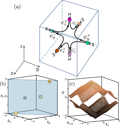
Figure 1: (Color online) (a) One unit cell of the 3D network model. The thick black lines are directed links, with the arrows indicating the directions of wave propagation. The colored circles represent coupling nodes, lying at the center of each face of the cube. The incident wave amplitudes are labeled $\psi_{\mu}^{\pm}$. (b) Weyl point positions in $k$-space, for $\theta_{x}=\theta_{y}=\pi/8$, $\theta_{z}=3\pi/8$. The Weyl points consist of two pairs, at $\phi=0$ and $\phi=\pi$, all lying on the plane $k_{x}=k_{y}$ (shaded region). Each Weyl point is labeled by its topological charge. (c) The quasienergy bandstructure plotted along the $k$-space cross section $k_{x}=k_{y}$.

The network model of interest is shown schematically in Fig. 1(a). It consists of directed links along which waves can propagate, joined by coupling nodes. The links and nodes form a periodic 3D cubic lattice, with six links per unit cell. The links terminate at nodes located at the center of the various faces of the cube. Each node thus connects two incoming links, from adjacent unit cells, to two outgoing links. The wave amplitude at each point along a link is given by a complex scalar.

This 3D network generalizes the 2D square-lattice network model originally introduced by Chalker and Coddington for studying quantum Hall systems ChalkerCo . For the 2D network in the weak-coupling limit, the links in each unit cell form a closed directed loop, analogous to the cyclotron orbits of 2D electrons in a magnetic field. In this 3D network, the links likewise form a directed chiral loop in the 3D unit cell, in a way that treats the $x$, $y$, and $z$ directions on similar footing. In 2D, Ho and Chalker have previously shown that the Floquet bandstructure exhibits 2D Dirac states when tuned to a critical point HoChalker ; analogously, the 3D network model exhibits Weyl phases.

Chalker and Dohmen ChalkerDohmen have previously studied a 3D network model consisting of stacked 2D Chalker-Coddington networks. For weak inter-layer coupling, their network model behaves as a 3D generalization of a quantum Hall insulator, which would nowadays be called a $\mathcal{T}$-broken weak topological insulator. We shall show that our model possesses several different insulator phases, which can be interpreted as either conventional insulators or distinct Chalker-Dohmen insulators with different choices of weak axis. The relationships between these insulator phases, and the Weyl phases separating them, will be explored in Section IV.

Within a given unit cell, let $\psi_{\mu}^{\pm}$ denote the wave amplitude incident on a node located along the $\mu$ direction, where $\mu\in\{x,y,z\}$ and $\pm$ denotes the node on the positive or negative side of axis $\mu$. These are labeled in Fig. 1(a). Likewise, let $\varphi_{\mu}^{\pm}$ denotes the wave amplitude exiting the node located on the $\pm\mu$ axis. Let each of the links be associated with an equal line delay $\phi/3$, so that

$$\psi_{z}^{+}=e^{i\phi/3}\varphi_{y}^{-},\;\;\psi_{x}^{-}=e^{i\phi/3}\varphi_{z}^{+},\;\;\mathrm{etc.}$$ (1)

For an infinite network, propagating waves can be decomposed into Bloch modes. At each node, the incoming and outgoing wave amplitudes are related by a $2\times 2$ unitary coupling relation

$$\begin{pmatrix}\varphi_{\mu}^{-}\,e^{ik_{\mu}}\\ \varphi_{\mu}^{+}\\ \end{pmatrix}=\begin{pmatrix}\sin\theta_{\mu}&i\cos\theta_{\mu}\\ i\cos\theta_{\mu}&\sin\theta_{\mu}\\ \end{pmatrix}\begin{pmatrix}\psi_{\mu}^{+}\\ \psi_{\mu}^{-}e^{ik_{\mu}}\\ \end{pmatrix},$$ (2)

where $k_{\mu}\in[-\pi,\pi)$ is the quasimomentum, in units of the inverse lattice period. For convenience, we use simple unitary $2\times 2$ coupling matrices corresponding to couplers that are symmetric under $180^{\circ}$ rotations Liang ; Liang2014 . The angle parameter $\theta_{\mu}\in[-\pi,\pi)$ denotes the coupling strength along the $\mu$ direction; $\theta_{\mu}=0$ corresponds to decoupling adjacent cells. (As discussed in Appendix A, generalizing the coupling matrix to a full $2\times 2$ unitary matrix, by including three more Euler angles, leads to trivial translations of the bands.)

Combining Eqs. (1)–(2) yields the eigenvalue problem

$$U(k)\Psi(k)=e^{-i\phi(k)}\Psi(k),$$ (3)

where $\Psi=[\psi_{z}^{+},\psi_{z}^{-}]^{\text{T}}$, and $U$ is a $2\times 2$ unitary matrix depending on $\{k_{\mu},\theta_{\mu}\}$. Details are given in Appendix A.

We regard $\phi(k)$ as a quasienergy HoChalker ; Liang ; Yidong2014 , analogous to the band energy of a crystal except that it is an angle with $2\pi$ periodicity. If the network is realized using electromagnetic waveguides for the links Liang ; Yidong2014 ; Yidong2015 ; Gao , the quasienergy is fixed by the phase delay of the waveguides; this is analogous to probing one single frequency in a photonic crystal, or one energy (e.g. the Fermi level) in an electronic system. Depending on the experimental realization, it may also be possible to vary $\phi$ continuously, e.g. by tuning the operating frequency to alter the phase delay in the waveguides. Alternatively, $U(k)$ can also be derived as the Floquet operator of a 3D discrete-time quantum walk, as described in Appendix C. In the quantum walk context, $\phi(k)$ describes the temporal periodicity of a Floquet eigenmode Tanaka2010 ; Kitagawa2010 ; Lindner2011 ; Gong2012 ; MLevin2013 ; it is usually difficult to select a specific quasienergy, and instead one excites a specific quasimomentum or lattice position, which generates a superposition of Floquet eigenmodes Rechtsman .

By analytically diagonalizing $U$, we find that the 3D parameter space $(\theta_{x},\theta_{y},\theta_{z})$ is divided into three sets of phases: (a) an octahedron with vertices at $(\pm\frac{\pi}{2},\pm\frac{\pi}{2},\pm\frac{\pi}{2})$, corresponding to a conventional insulator; (b) eight tetrahedra with bases lying on each face of the (a) octahedron and vertices at $\theta_{\mu}=\pm\pi$, corresponding to gapless Weyl phases; and (c) the regions outside (a) and (b), which form three octahedra (modulo $\pi$ in the $\theta_{\mu}$ parameters), and turn out to be weak topological insulators. We first focus on the Weyl phases; the insulator phases will be explored in Section IV.

In each Weyl phase, the bandstructure is completely gapless: the quasienergy bands are connected by simultaneous band-crossing points, such that there is no gap at any quasienergy $\phi\in[-\pi,\pi)$. (A similar phenomenon has previously been seen in critical 2D Floquet bandstructures Yidong2014 ; Tauber .) There are two pairs of band-crossing points. One pair occurs at quasienergy $\phi=\pi$ and $k=\pm\bar{k}$; the analytic expressions for $\{\bar{k}_{x},\bar{k}_{y},\bar{k}_{z}\}$ in terms of $\{\theta_{x},\theta_{y},\theta_{z}\}$ are given in Appendix A. The other pair occurs at quasienergy $\phi=0$ and $k=\pm(\bar{k}-\pi)$. Fig. 1(b) shows the $k$-space positions of the band-crossing points (Weyl points) for $\theta_{x}=\theta_{y}=\pi/8$, $\theta_{z}=3\pi/8$, and Fig. 1(c) shows the quasienergy bandstructure.

Near the Weyl point at $\bar{k}$, we can expand the evolution matrix as $U(\bar{k}+\kappa)=e^{-iH_{\text{eff}}}$, where

$$H_{\text{eff}}(\kappa)=\nu_{ij}\kappa_{i}\sigma_{j},\;\;\;\nu_{ij}\in\mathbb{R}.$$ (4)

This is the Weyl Hamiltonian describing a massless relativistic particle; similar expansions can be performed around each of the other three Weyl points. The $\nu$ matrix satisfies

$$\det[\nu_{ij}]=-\sin\theta_{z}\sin{\bar{k}_{z}}\\ \times\left(\cos\theta_{y}\sin\theta_{z}\cos{\bar{k}_{z}}+\cos\theta_{z}\sin\theta_{y}\cos{\bar{k}_{y}}\right)\\ \times\left(\cos\theta_{x}\sin\theta_{z}\cos{\bar{k}_{z}}+\cos\theta_{z}\sin\theta_{x}\cos{\bar{k}_{x}}\right).$$ (5)

Each Weyl point is associated with a topological charge, consisting of the Berry flux of a band integrated over a $k$-space sphere surrounding the point. This takes values ${\text{sgn}}(\det[\nu_{ij}])=\pm 1$, representing the chirality of the Weyl particles Hosur2013 . (It is also necessary to choose which band’s Berry flux to put into the calculation; we adopt the convention of using the band below each Weyl point.) Each two Weyl points at the same quasienergy have opposite chiralities, consistent with the principle that the total chirality sums to zero (the Nielsen-Ninomiya theorem) Nielsen1981a ; Nielsen1981b .

The locations and chiralities of the Weyl points are constrained by the symmetries of $U(k)$. According to Kitagawa et al.’s classification of Floquet operator symmetries Kitagawa2010 , a system is time-reversal ($\mathcal{T}$) symmetric if $U^{\dagger}=\mathcal{Q}\,U^{*}\,\mathcal{Q}^{\dagger}$, where $\mathcal{Q}$ is some unitary operator; and it is particle-hole symmetric if $U=\mathcal{P}U^{*}\mathcal{P}^{\dagger}$ for some unitary $\mathcal{P}$. Our network model breaks $\mathcal{T}$ due to the directed nature of the network (Fig. 1), and this can be verified from the fact that $U^{\dagger}$ and $U^{*}$ have different spectra. On the other hand,

$$U(k)=\sigma_{y}U^{*}(k)\sigma_{y},$$ (6)

corresponding to a particle-hole symmetry with $\mathcal{P}=i\sigma_{y}$. For every eigenstate at quasienergy $\phi$ and momentum $k$, there is an eigenstate at $-\phi$ at the same $k$. Thus, Weyl points can only occur at $\phi=0$ and $\phi=\pi$. We can also conclude that chiral symmetry is broken Ryu2010 .

The network model also satisfies inversion symmetry:

$$U(-k)=\sigma_{x}U(k)\sigma_{x}.$$ (7)

This explains why the Weyl points occur in pairs, at $k$ and $-k$, with opposite chiralities.

There is one more interesting symmetry of $U(k)$:

$$U(k)=-\sigma_{z}\,U\!\left(k+[\pi,\pi,\pi]\right)\,\sigma_{z}.$$ (8)

Thus, for every eigenstate at quasienergy $\phi$ and momentum $k$, there is an eigenstate at $\phi+\pi$ and $k+[\pi,\pi,\pi]$. This, together with the particle-hole symmetry, guarantees that Weyl points at $\phi=0$ and $\phi=\pi$ occur simultaneously. (A similar phenomenon occurs in the 2D network model Tauber , though in 2D the gap-closings occur only at critical points.) Thus, the Weyl point at $\phi=\pi$ and $k=\bar{k}$ has the same chirality as the one at $\phi=0$ and $k=-(\bar{k}-[\pi,\pi,\pi])$, and likewise for the other pair.

Eqs. (6)–(8) hold for a network in which the node couplings have the highly symmetric form given by Eq. (2). Adopting more general node couplings will shift the bandstructure in $\phi$ and/or $k$, as discussed in Appendix A. This correspondingly modifies the symmetry relations; in particular, the Weyl points may move away from the special quasienergies ($\phi=0$ and $\phi=\pi$) and $k$-space plane on which they were previously constrained, without lifting the band degeneracies of the Weyl points themselves.

III Fermi arc surface sates

Weyl points in a bulk bandstructure have a topological correspondence with the existence, in a truncated lattice, of “Fermi arc” surface states. At a given energy, these surface states lie along an open arc in the projected 2D $k$-space, connecting a pair of Weyl cones ZFang2011 ; SMYoung . This is fundamentally different from ordinary 2D bands, which must form closed $k$-space loops, and is possible only because the surface states lie on the boundary of a 3D bulk.

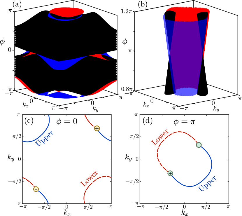
Figure 2: (Color online) (a) Quasienergy bandstructure for the 3D network in a slab geometry with thickness $N=16$. The coupling parameters are $\theta_{x}=\theta_{y}=\pi/8$, $\theta_{z}=3\pi/8$. (b) Close-up view of the bandstructure near $\phi=\pi$, showing bulk Weyl cones and Fermi arc surface states. (c)–(d) Cross sections of the bandstructure at (c) $\phi=0$, and (d) $\phi=\pi$; circles indicate Weyl points with positive ($+$) and negative ($-$) topological charges, calculated using the Berry flux on the band below each Weyl point.

To confirm that the gapless phases of the network model are Weyl phases, we have numerically calculated the surface states and observed the presence of Fermi arcs. Details of the calculation are given in Appendix B. Essentially, we impose a “slab” geometry by truncating the 3D network to $N$ periods along $z$, while keeping it infinite and periodic in $x$ and $y$ directions with quasimomentum $(k_{x},k_{y})$. Wave amplitudes in adjacent cells are related by

$$M\begin{pmatrix}\varphi_{z}^{-}(j)\\ \psi_{z}^{-}(j)\\ \end{pmatrix}=\begin{pmatrix}\varphi_{z}^{-}(j+1)\\ \psi_{z}^{-}(j+1)\\ \end{pmatrix},$$ (9)

where $j$ is the position index along $z$, and $M$ is a transfer matrix that depends on $(k_{x},k_{y})$, $\phi$, and $\{\theta_{\mu}\}$. We impose Dirichlet boundary conditions by setting $\psi_{z}^{-}=\varphi_{z}^{-}$ on cell $j=1$ (the bottom surface), and $\psi_{z}^{+}=\varphi_{z}^{+}$ on cell $j=N$ (the upper surface). We then calculate the bandstructure by searching for values of $\phi$ consistent with the boundary conditions, for each $(k_{x},k_{y})$ in the 2D Brillouin zone.

The results are shown in Fig. 2. Fig. 2(a) shows the entire bandstructure, with bulk bands plotted in black and the surface state bands for the upper (lower) surface plotted in blue (red). Fig. 2(b) represents the portion of the bandstructure near $\phi=\pi$, clearly showing the existence of two Weyl cones, to which the surface states are attached along Fermi arcs. Fig. 2(c) and (d) plot cross-sections taken at the Weyl point quasienergies $\phi=0$ and $\phi=\pi$, showing how each Fermi arc connects a pair of Weyl points with opposite chiralities.

In the condensed matter setting, Fermi arc states have been predicted to exhibit novel behaviors, including quantum oscillations in magnetotransport and quantum interference effects in tunneling spectroscopy Hosur2013 ; Burkov2015 . If the present model is implemented using a electromagnetic network, however, most of the previously-identified experimental signatures will be unavailable due to the absence of a Fermi level. In the next section, we discuss a different approach to probing the topological structure of the Weyl phase, based on reflection measurements.

IV Topological Invariants

In order to clarify the nature of the gapped phases, we seek to formulate topological invariants for the various phases of the network model. A standard way to characterize gapped 3D phases is to calculate a triplet of Chern numbers obtained by integrating the Berry flux across sections of the 3D Brillouin zone corresponding to the $yz$, $zx$ and $xy$ planes Avron1983 ; Moore2007 ; HasanRMP2010 . For example, integrating across the $yz$ plane gives

$$\nu_{x}^{n}=\frac{1}{2\pi}\oiint B_{n}(k)\cdot ds_{yz},$$ (10)

where $B_{n}(k)=\nabla_{k}\times A(k)$ is the Berry curvature and $A_{n}(k)=i\langle\Psi_{nk}|\nabla_{k}|\Psi_{nk}\rangle$ is the Berry connection evaluated on band $n$, computed using bulk Bloch functions. By the Gauss-Bonnet theorem, any such integral taken over a closed 2D surface must give an integer.

For all the gapped phases of the network model, we find that $\nu_{x}^{n}=\nu_{y}^{n}=\nu_{z}^{n}=0$, which ordinarily indicates that these phases are topologically trivial. However, Chern number invariants can be misleading in characterizing Floquet bandstructures. In 2D, it has previously been shown that an anomalous Floquet insulator phase can exist which is topologically non-trivial but has zero Chern numbers in all bands Kitagawa2010 ; MLevin2013 ; Yidong2014 , with the topological non-triviality verified by the existence of protected edge states. Roughly speaking, the anomalous Floquet insulator phase arises by applying band inversions in every gap of the conventional insulator, including the gap which “wraps around” the quasienergy $\phi$ (which is an angle variable). This phenomenon is unique to Floquet systems, and cannot occur with static Hamiltonians. As we now argue, a similar phenomenon occurs in the 3D network model, so that there are actually four topologically distinct gapped phases which cannot be distinguished using Chern number triplets.

To characterize these gapped phases, we introduce a “topological pumping” process Brouwer1998 ; Brouwer2011 ; Fulga ; Fulga2015 . As originally introduced by Brouwer et al. Brouwer1998  for 2D systems, the idea is to roll a lattice into a cylinder with tunable phase slip $k$ along the azimuthal direction, and attach scattering leads to the ends of the cylinder. When the cylinder length greatly exceeds the attenuation length for the bulk gap, the scattering matrix reduces to two unitary blocks, $r_{\pm}$, which are the reflection matrices off each end. The topological invariant is the integer winding number of the reflection phase,

$$-i\ln\left[\det{r_{\pm}}\right],$$

as $k$ advances through $2\pi$. This concept can be applied directly to 2D network models, and has been used to experimentally distinguish between topological phases of a microwave network Yidong2015 .

We apply the topological pumping procedure to the 3D network model in the following way: consider the slab geometry from Section III, with $N$ cells stacked in the $z$ direction and wave-vector $(k_{x},k_{y})$. Using the transfer matrix relation in Eq. (9), we derive a scattering relation

$$\mathcal{S}(k_{x},k_{y},\phi,N)\begin{pmatrix}\psi_{z}^{+}(N)\\ \psi_{z}^{-}(1)\\ \end{pmatrix}=\begin{pmatrix}\varphi_{z}^{+}(N)\\ \varphi_{z}^{-}(1)\\ \end{pmatrix},$$ (11)

which relates the wave amplitudes on the upper and lower surfaces. In the large-$N$ limit, if $\phi$ falls into a quasienergy gap, the scattering matrix becomes purely reflecting:

$$\mathcal{S}\rightarrow\begin{pmatrix}e^{i\omega_{+}}&0\\ 0&e^{i\omega_{-}}\end{pmatrix}.$$ (12)

We then pick one of the diagonal entries, say the one corresponding to reflection off the lower surface, and determine how its phase winds with $k_{x}$ and $k_{y}$. (The other surface will have the opposite windings.) This process can be repeated for slabs taken perpendicular to the $x$ and $y$ directions.

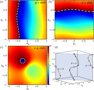
Figure 3: (Color online) (a)–(c) Heat maps of the reflection phase $\omega_{-}$ in a gapped phase. We take $\theta_{x}=\theta_{y}=3\pi/8$ and $\theta_{z}=\pi/8$ [green star in Fig. 5(a)], and quasienergy $\phi=\pi$. The slab is taken in the (a) $y$-$z$, (b) $x$-$z$, and (c) $x$-$y$ planes. Dashed lines are contours of $\omega_{-}=0$. (d) Trajectory of the Weyl points when traversing a Weyl phase from a $(0,0,0)$ conventional insulator phase to a $(0,0,1)$ weak topological insulator phase, along the path indicated in Fig. 5(a).

Fig. 3(a)–(c) shows the reflection phase $\omega_{-}$ versus $k_{\mu}$, using the parameters $\theta_{x}=\theta_{y}=3\pi/8$ and $\theta_{z}=\pi/8$. The $y$-$z$ slab exhibits winding number $+1$ in the $k_{y}$ direction, and the $x$-$z$ slab exhibits winding number $-1$ in the $k_{x}$ direction. The winding in the $k_{z}$ direction is zero for these slabs, and for the $x$-$y$ slab it is zero in both $k_{x}$ and $k_{y}$. The reflection phase on the upper surface, $\omega_{+}$, has opposite windings from what is shown here.

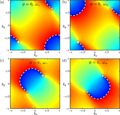
Figure 4: (Color online) Heat maps of the reflection phases $\omega_{\pm}$ in a Weyl phase. We take $\theta_{x}=\theta_{y}=\pi/8$ and $\theta_{z}=3\pi/8$ [blue star in Fig. 5(a)], and an $x$-$y$ slab. In (a) and (b), we fix the quasienergy at $\phi=0$ and plot (a) the reflection phase $\omega_{-}$ off the lower surface, and (b) the reflection phase $\omega_{+}$ off the upper surface. In (c) and (d), we fix the quasienergy at $\phi=\pi$ and plot (c) $\omega_{-}$ and (d) $\omega_{+}$. The projection of each Weyl point onto the plane coincides with a phase singularity; the circles labeled $\pm$ indicate the Weyl point’s topological charge. The dashed lines are contours of $\omega_{\pm}=0$.

The topological pumping process can also be carried out in the Weyl phase. We can fix $\phi$ at quasienergy $0$ or $\pi$, corresponding to one pair of Weyl points, and plot the reflection phase map. Fig. 4 shows the results for $\theta_{x}=\theta_{y}=\pi/8$ and $\theta_{z}=3\pi/8$, and an $x$-$y$ slab. At two specific $k$ points, corresponding to the projection of the Weyl points onto the plane, the system is gapless, and Eq. (12) breaks down since the slab is not purely reflecting. Everywhere else in the 2D Brillouin zone, the system is gapped and Eq. (12) holds, so that $\omega_{\pm}$ is well-defined. In the resulting reflection phase map, the $k$ points corresponding to the Weyl point projections are associated with phase singularities; the phase winds by $\pm 2\pi$ around each singularity, and is ill-defined at the singularity itself. For $\omega_{+}$ (reflection off the upper surface), the winding number of each phase singularity—using right-handed coordinates, and treating anti-clockwise winding as positive—is equal to the Weyl point’s topological charge as computed from its Berry flux (Section II). For $\omega_{-}$ (the lower surface), the winding numbers and topological charges have opposite signs. This holds at both Weyl point quasienergies.

The reflection phase singularities are intimately related to the phenomenon of Fermi arcs. The phase singularities can be joined by equal-phase contours, and the contours for $\omega_{\pm}=0$ (shown as dashes in Fig. 4) exactly match the Fermi arc surface states plotted in Fig. 2(c)–(d). This is because the Fermi arc surface states arise from Dirichlet boundary conditions that are equivalent to setting $\omega_{\pm}=0$ in the topological pump.

Based on the above discussion, the windings of the reflection phase in each gapped phase can be characterized by an integer triplet, the “pumping invariant” $\vec{n}=(n_{x},n_{y},n_{z})$. This is defined as follows: for the slab with normal vector $\hat{s}$,

$$(\text{winding in direction}\;\hat{\mu})\;=\;\pm\,(\hat{s}\times\vec{n})\cdot\hat{\mu},$$ (13)

where $\pm$ corresponds to the choice of $\omega_{\pm}$ (i.e., upper or lower surface). Both quasienergy gaps give the same value for $(n_{x},n_{y},n_{z})$.

Fig. 5 shows the topological phase diagram of the network model, with the gapped phases classified using the pumping invariants. For ease of visualization, we have reduced the parameter space to 2D by taking the section $\theta_{x}=\theta_{y}$ in Fig. 5(a), and $\theta_{z}=\pi/4$ in Fig. 5(b). The white regions are gapped phases with invariants $(0,0,0)$, corresponding to conventional insulators. The pink regions are topologically non-trivial gapped phases, which fall into three groups with either $n_{x}$, $n_{y}$, or $n_{z}$ non-zero. The cyan regions are the Weyl phases. Note that any transition between different gapped phases requires passing through a Weyl phase.

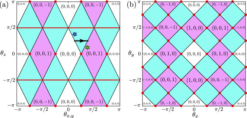
Figure 5: (Color online) Phase diagram of the 3D network for two different sections of the parameter space $\{\theta_{x},\theta_{y},\theta_{z}\}$: (a) $\theta_{x}=\theta_{y}$ and (b) $\theta_{z}=\pi/4$. The white regions are conventional insulator phases; the pink regions are $\mathcal{T}$-broken weak topological insulator phases characterized by nonzero winding number triplets $(n_{x},n_{y},n_{z})$; and the cyan regions are gapless Weyl phases. Along the red lines and dots, the band-touching points form line nodes. The dotted line is the path producing the Weyl point trajectories in Fig. 3(d). Green and blue stars indicate the parameters for Fig. 3 and Fig. 4, respectively.

Consider the $(0,0,1)$ phase. It has a topologically protected surface state if the slab is taken in the $x$-$z$ or $y$-$z$ direction. This follows from the fact that $\omega_{\pm}=0$ corresponds to the Dirichlet boundary conditions for a surface state calculation (see Section III). This behavior is reminiscent of “weak topological insulator” phases Fu2007 , and hence we refer to the topologically nontrivial gapped phases as such. (Note, however, that the “weak topological insulator” terminology was originally introduced in the context of $\mathcal{T}$ symmetric materials, whereas $\mathcal{T}$ is broken in this model.) The gapped phase can be adiabatically continued to a stack of 2D sheets, similar to the Chalker-Dohmen model ChalkerDohmen . In fact, each sheet is a 2D anomalous Floquet topological insulator Kitagawa2010 ; MLevin2013 ; Yidong2014 , which has the unique feature that the winding-number invariant is the same in all quasienergy gaps Yidong2014 . This is consistent with above-mentioned finding that the $(n_{x},n_{y},n_{z})$ invariant is gap-independent.

The pumping invariant $(n_{x},n_{y},n_{z})$ was derived in terms of the winding numbers of the reflection phase in the 2D Brillouin zone. However, they can also be related to the winding numbers of the Weyl point trajectories. We can regard the gapped phases as being “generated” via Weyl phases by the mutual annihilation of Weyl points. In this view, the different types of trajectories undertaken by the Weyl points, between creation and annihilation, give rise to the various topologically-distinct gapped phases Murakami2008 .

To illustrate this, consider a parameter-space trajectory from a $(0,0,0)$ conventional insulator to a $(0,0,1)$ weak topological insulator, transiting through a Weyl phase as indicated by the dotted arrow in Fig. 5(a). The trajectories of the Weyl points under this parameter evolution are plotted in Fig. 3(d). Throughout, the Weyl points lie in the plane $k_{x}=k_{y}$. At the boundary with the conventional insulator, a pair of Weyl points with opposite chiralities is generated at $k=[0,0,0]$ with quasienergy $\phi=\pi$, and another pair is generated at $k=[\pi,\pi,\pi]$ with quasienergy $\phi=0$. As the system transits through the Weyl phase, the Weyl points move across the Brillouin zone and recombine once the system reaches the phase boundary with the $(0,0,1)$ phase.

Based on this, we can define a net winding number

$$\Delta n_{\mu}=-\frac{1}{2\pi}\sum_{c\in\pm 1}c\int_{0}^{1}d\lambda\,\frac{dk^{\mu}_{c}}{d\lambda},$$ (14)

where $k^{\mu}_{c}(\lambda)$ denotes the $k$-space position of the Weyl point with topological charge $c$, and $\lambda\in[0,1]$ is a path parameter whose endpoints correspond to phase boundaries with gapped phases. Assuming $\lambda=0$ is a conventional insulator, $(\Delta n_{x},\Delta n_{y},\Delta n_{z})$ is precisely equal to the pumping invariant $(n_{x},n_{y},n_{z})$ for the gapped phase at $\lambda=1$. This follows from the earlier observation that a Weyl point with topological charge $c$ produces a phase singularity with winding number $\pm c$ (on the $\pm$ surface).

A similar sort of winding behavior was previously noted by Murakami and Kuga Murakami2008 , in the context of 3D quantum spin Hall systems. They found that crossing a Weyl phase between two spin Hall insulators, such as a weak and strong topological insulator, produced a $k$-space motion of two pairs of Weyl points. Rather than wrapping around the Brillouin zone, as in the present network model, the Weyl points encircled a time-reversal invariant momentum point, and the net winding could be linked to a $Z_{2}$ topological number Murakami2008 .

V Discussion

In this paper, we have described a 3D network model exhibiting Weyl, conventional insulator, and $\mathcal{T}$-broken weak topological insulator phases. The 3D model is closely related to previously-studied 2D network models Liang ; Yidong2014 ; Yidong2015 ; Tauber ; specifically, the weak topological insulator phases can be adiabatically continued to a stack of decoupled 2D anomalous Floquet insulators (which are “anomalous” because their bandstructures are topologically non-trivial despite all bands having zero Chern number Kitagawa2010 ; MLevin2013 ; Gong2014 ). Our study relied in part on the “topological pumping” invariant, which relates bandstructure topology to reflection coefficients Brouwer1998 ; Brouwer2011 ; Fulga ; Fulga2015 . Though this method was originally developed with topological insulators in mind, we have shown that it has interesting applications to Weyl phases: the Weyl points produce phase singularities in the reflection spectrum, associated with the Fermi arc surface states SMYoung ; Fermi_note . From this, we found an intriguing correspondence between the topology of the insulator phases, and the $k$-space topology of Weyl point trajectories as they wind around the Brillouin zone. In this view, the various insulator phases are generated through the creation and annihilation of Weyl point pairs with different $k$-space windings.

A promising route to realizing the network model is to use coupled microwave components, similar to the experiment reported in Ref. Yidong2015, which realized a 2D topological pump acting on an anomalous Floquet insulator. The network links would be microwave lines (e.g. coaxial cables), with line delays fixed at $\phi=0$ or $\phi=\pi$ (the Weyl point quasienergies). The nodes would be four-port couplers, with isolators to enforce directionality. Rather than implementing a large slab, tunable phase-shifters can simulate Bloch boundary conditions Yidong2015 , using two sets of phase-shifters corresponding to (e.g.) $k_{x}$ and $k_{y}$. The key experimental signatures would be the phase singularities, and their $k$-space trajectories, as discussed in Section IV. Although an electromagnetic Weyl phase has previously been realized LLu2013 , that photonic crystal-based experiment was unable to probe the topological features of the Weyl points. Our proposed approach would demonstrate the topological robustness of the Weyl points through their association with phase singularities. This requires measuring complex wave parameters (i.e., including phase information), which is achievable with microwave vector network analyzers Yidong2015 ; Gao .

The network model that we have chosen to study is, in a sense, the simplest non-trivial design that generalizes the Chalker-Coddington 2D network model to 3D, while maintaining similar network topology in the $x$, $y$, and $z$ directions. We have focused on studying various interesting properties of the disorder-free network; however, it is worth noting that the original motivation of network models was to provide a computationally efficient method for studying the effects of disorder ChalkerCo . In future work, we intend to investigate whether such 3D network models can be used to model disordered Weyl semimetals. 3D network models with more complicated network topologies may also exhibit other topological phases remaining to be explored. It might also be interesting to realize static (non-Floquet) Hamiltonian models that can exhibit the phenomenon of Weyl point trajectories winding around the Brillouin zone.

We thank W. Hu, D. Leykam, C. Huang, P. Chen, B. Zhang, and L. Lu for helpful comments. This research was supported by the Singapore National Research Foundation under grant No. NRFF2012-02, and by the Singapore MOE Academic Research Fund Tier 3 grant MOE2011-T3-1-005.

Appendix A 3D network bandstructure

This appendix describes the derivation of the evolution matrix characterizing the network model introduced in Section II. As previously discussed, in each unit cell the amplitudes entering the nodes are $\psi_{\mu}^{\pm}$, and those leaving the nodes are $\varphi_{\mu}^{\pm}$. For Bloch modes, the scattering relations are given in Eq. (2). This can be re-arranged as

$$\begin{pmatrix}\varphi_{\mu}^{-}\\ \varphi_{\mu}^{+}\\ \end{pmatrix}=\begin{pmatrix}e^{-ik_{\mu}}\sin\theta_{\mu}&i\cos\theta_{\mu}\\ i\cos\theta_{\mu}&e^{ik_{\mu}}\sin\theta_{\mu}\\ \end{pmatrix}\begin{pmatrix}\psi_{\mu}^{+}\\ \psi_{\mu}^{-}\\ \end{pmatrix}\;.$$ (15)

On the other hand, the wave amplitudes are also related by the fact that traversing each link incurs a phase delay of $\phi/3$. Thus (referring to Fig. 1):

$$\begin{pmatrix}\psi_{z}^{+}\\ \psi_{z}^{-}\\ \end{pmatrix} =e^{i\frac{\phi}{3}}\begin{pmatrix}\varphi_{y}^{-}\\ \varphi_{y}^{+}\\ \end{pmatrix}$$ (16)

$$\begin{pmatrix}\psi_{y}^{+}\\ \psi_{y}^{-}\\ \end{pmatrix} =e^{i\frac{\phi}{3}}\begin{pmatrix}\varphi_{x}^{-}\\ \varphi_{x}^{+}\\ \end{pmatrix}$$ (17)

$$\begin{pmatrix}\psi_{x}^{+}\\ \psi_{x}^{-}\\ \end{pmatrix} =e^{i\frac{\phi}{3}}\begin{pmatrix}\varphi_{z}^{-}\\ \varphi_{z}^{+}\\ \end{pmatrix}\;.$$ (18)

Combining Eqs. (15)–(18) gives $U\Psi=e^{-i\phi}\Psi$, where

$$\begin{aligned} U&=U_{z}U_{y}U_{x},\\ U_{\mu}&\equiv\begin{pmatrix}e^{-ik_{\mu}}\sin\theta_{\mu}&i\cos\theta_{\mu}\\ i\cos\theta_{\mu}&e^{ik_{\mu}}\sin\theta_{\mu}\\ \end{pmatrix}.\end{aligned}$$ (19)

From its eigenvalues, we find the quasienergies

$$\begin{aligned} \phi=\pm\cos^{-1}\Big{[}&\cos(k_{x}+k_{y}+k_{z})\sin\theta_{x}\sin\theta_{y}\sin\theta_{z}\\ &-\cos k_{x}\sin\theta_{x}\cos\theta_{y}\cos\theta_{z}\\ &-\cos k_{y}\cos\theta_{x}\sin\theta_{y}\cos\theta_{z}\\ &-\cos k_{z}\cos\theta_{x}\cos\theta_{y}\sin\theta_{z}\Big{]}.\end{aligned}$$ (20)

The band-crossing points are determined by the degeneracies of the multiple-valued arc cosine, so either $\phi=\pi$ or $\phi=0$. For $\phi=\pi$, degeneracies occur at $\pm\bar{k}_{\mu}$, where

$$\begin{aligned} \bar{k}_{x}&=s_{x}\cos^{-1}\left(\frac{-\cos^{2}\theta_{x}+\cos^{2}\theta_{y}+\cos^{2}\theta_{z}}{2\sin\theta_{x}\cos\theta_{y}\cos\theta_{z}}\right)\\ \bar{k}_{y}&=s_{y}\cos^{-1}\left(\frac{\cos^{2}\theta_{x}-\cos^{2}\theta_{y}+\cos^{2}\theta_{z}}{2\cos\theta_{x}\sin\theta_{y}\cos\theta_{z}}\right)\\ \bar{k}_{z}&=-s_{z}\cos^{-1}\left(\frac{\cos^{2}\theta_{x}+\cos^{2}\theta_{y}-\cos^{2}\theta_{z}}{2\cos\theta_{x}\cos\theta_{y}\sin\theta_{z}}\right),\end{aligned}$$ (21)

where $s_{\mu}\equiv\text{sgn}(\sin 2\theta_{\mu})$. For $\phi=0$, degeneracies occur at $\pm(\bar{k}-[\pi,\pi,\pi])$.

Using Eqs. (19)–(21), we expand the evolution matrix in the vicinity of the Weyl point $\bar{k}$, as $U\approx e^{-iH_{\text{eff}}}$. To leading order in the displacement $\kappa=k-\bar{k}$, we find that $H_{\text{eff}}=\nu_{ij}\kappa_{i}\sigma_{j}$, with coefficients

$$\begin{array}[]{ll}\nu_{xx}&=-g_{yz}\sin\bar{k}_{x}\\ \nu_{xy}&=\;\;\;g_{yz}\cos\bar{k}_{x}\\ \nu_{xz}&=\;\;\;g_{yz}\tan\theta_{x}\\ \end{array},\quad\begin{array}[]{ll}\nu_{yx}&=-g_{xz}\sin\bar{k}_{y}\\ \nu_{yy}&=-g_{xz}\cos\bar{k}_{y}\\ \nu_{yz}&=\;\;\;g_{xz}\tan\theta_{y}\\ \end{array}$$

$$\;\nu_{zx}\;=-\left[f_{x}\sin(\bar{k}_{y}+\bar{k}_{z})+f_{y}\sin(\bar{k}_{x}+\bar{k}_{z})\right]$$

$$\;\nu_{zy}\;=-\left[f_{x}\cos(\bar{k}_{y}+\bar{k}_{z})-f_{y}\cos(\bar{k}_{x}+\bar{k}_{z})\right]$$

$$\;\nu_{zz}\;=-\cos\theta_{x}\cos\theta_{y}\sin\theta_{z}\cos\bar{k}_{z}$$

$$\quad\qquad-\sin\theta_{x}\sin\theta_{y}\sin\theta_{z}\cos(\bar{k}_{x}+\bar{k}_{y}+\bar{k}_{z}),$$

where

$$\begin{aligned} g_{\mu\nu}&\equiv\sin\theta_{x}\sin\theta_{y}\sin\theta_{z}\left(\frac{\cos\bar{k}_{\nu}}{\tan\theta_{\mu}}+\frac{\cos\bar{k}_{\mu}}{\tan\theta_{\nu}}\right)\\ f_{\mu}&\equiv\frac{\sin\theta_{x}\sin\theta_{y}\sin\theta_{z}}{\tan\theta_{\nu}}.\end{aligned}$$ (22)

From this, Eq. (5) can be derived via direct substitution.

We have thus far assumed that the coupling matrices at the nodes have the simple form given in Eq. (2), corresponding to couplers with $180^{\circ}$ rotational symmetry Liang ; Liang2014 . The discussion can be generalized to arbitrary $2\times 2$ unitary coupling matrices of the form

$$\mathcal{U}_{c}=e^{i\Phi_{3}^{\mu}}\begin{pmatrix}\sin\theta_{\mu}e^{-i(\Phi_{1}^{\mu}+\Phi_{2}^{\mu})}&i\cos\theta_{\mu}e^{i(\Phi_{1}^{\mu}-\Phi_{2}^{\mu})}\\ i\cos\theta_{\mu}e^{-i(\Phi_{1}^{\mu}-\Phi_{2}^{\mu})}&\sin\theta_{\mu}e^{i(\Phi_{1}^{\mu}+\Phi_{2}^{\mu})}\\ \end{pmatrix},$$ (23)

where $\{\Phi_{1}^{\mu},\Phi_{2}^{\mu},\Phi_{3}^{\mu}\}$ are additional Euler angles which had previously been ignored (set to zero). With this generalization, the preceding results (15)–(22) still hold, subject to the replacement

$$\begin{aligned} \phi&\rightarrow\phi+\Phi_{3}^{x}+\Phi_{3}^{y}+\Phi_{3}^{z}\\ k_{x}&\rightarrow k_{x}-\Phi_{1}^{x}-\Phi_{2}^{x}-\Phi_{1}^{y}+\Phi_{2}^{y}+\Phi_{1}^{z}-\Phi_{2}^{z}\\ k_{y}&\rightarrow k_{y}+\Phi_{1}^{x}-\Phi_{2}^{x}-\Phi_{1}^{y}-\Phi_{2}^{y}-\Phi_{1}^{z}+\Phi_{2}^{z}\\ k_{z}&\rightarrow k_{z}-\Phi_{1}^{x}+\Phi_{2}^{x}+\Phi_{1}^{y}-\Phi_{2}^{y}-\Phi_{1}^{z}-\Phi_{2}^{z}.\end{aligned}$$ (24)

In other words, the Euler angles $\Phi_{1}^{\mu}$ and $\Phi_{2}^{\mu}$ translate the quasienergy bandstructure in $k$-space, whereas the Euler angle $\Phi_{3}^{\mu}$ translates it in $\phi$ (thus, for $\Phi_{2}^{\mu}\neq 0$, Weyl points would no longer occur at $\phi=0$ and $\phi=\pi$). Such translations do not, however, alter the topological properties of the network bandstructure.

Appendix B Bandstructures of finite-thickness slabs

To obtain the bandstructure of a finite-thickness slab (Section III), and the topological pumping invariants (Section IV), we need to calculate the transfer matrix for crossing the network in each direction. Consider the transfer matrix in $z$ (the other two transfer matrices are worked out similarly): the network is infinite and periodic in $x$ and $y$ directions, with quasimomenta $(k_{x},k_{y})$. The transfer matrix across one unit cell in the $z$ direction is defined by

$$M\begin{pmatrix}\varphi_{z}^{-}(j)\\ \psi_{z}^{-}(j)\\ \end{pmatrix}=\begin{pmatrix}\varphi_{z}^{-}(j+1)\\ \psi_{z}^{-}(j+1)\\ \end{pmatrix},$$ (25)

where $j$ and $j+1$ are adjacent cell indices along $z$. We can find $M$ using the network model definitions, as follows. Firstly, based on Eq. (2), we can relate the amplitudes at the bottom of cell $j+1$ to those at the top of cell $j$ by

$$\begin{aligned} M^{\prime}\begin{pmatrix}\psi_{z}^{+}(j)\\ \varphi_{z}^{+}(j)\end{pmatrix}&=\begin{pmatrix}\varphi_{z}^{-}(j+1)\\ \psi_{z}^{-}(j+1)\end{pmatrix},\\ \mathrm{where}\;\;M^{\prime}&\equiv\begin{pmatrix}\csc\theta_{z}&i\cot\theta_{z}\\ -i\cot\theta_{z}&\csc\theta_{z}\end{pmatrix}.\end{aligned}$$ (26)

Next, we use Eqs. (15)–(18) to relate $[\varphi_{z}^{+}(j),\psi_{z}^{+}(j)]^{\text{T}}$ to $[\varphi_{z}^{-}(j),\psi_{z}^{-}(j)]^{\text{T}}$, the amplitudes at the bottom of cell $j$. This introduces the phase delay $\phi/3$. The result is

$$M=\frac{1}{\chi}\begin{pmatrix}e^{i\phi}+\xi\cos\theta_{z}&i\left(e^{-i\phi}\cos\theta_{z}+\xi^{*}\right)\\ -i\left(e^{i\phi}\cos\theta_{z}+\xi\right)&e^{-i\phi}+\xi^{*}\cos\theta_{z}\end{pmatrix},$$

where

$$\xi \equiv e^{-ik_{x}}\sin\theta_{x}\cos\theta_{y}+e^{ik_{y}}\cos\theta_{x}\sin\theta_{y}$$

$$\chi \equiv\left[e^{i(k_{x}+k_{y})}\sin\theta_{x}\sin\theta_{y}-\cos\theta_{x}\cos\theta_{y}\right]\sin\theta_{z}.$$

From the one-cell transfer matrix $M$, we can calculate the transfer matrix across a stack of $N$ cells:

$$\mathcal{M}(N)=\left(M^{\prime}\right)^{-1}M^{N}.$$ (27)

This transfer matrix depends on the coupling parameters $\{\theta_{\mu}\}$, the transverse quasimomenta $(k_{x},k_{y})$, and the quasienergy $\phi$.

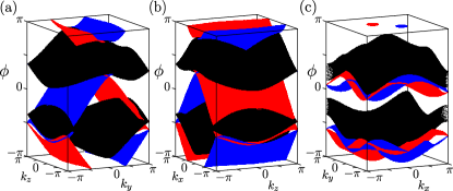
Figure 6: (Color online) Quasienergy bandstructure for the 3D network in various slab geometries: (a) $y$-$z$, (b) $x$-$z$, and (c) $x$-$y$. In all cases, the slab thickness is $N=16$, and the couplings are $\theta_{x}=\theta_{y}=3\pi/8$ and $\theta_{z}=\pi/8$, indicated by the green star in the phase diagram, i.e. a $(0,0,1)$ gapped phase.

To calculate the bandstructure of the slab, we search numerically for combinations of $\{\phi,k_{x},k_{y}\}$ such that $[1,1]^{\text{T}}$ is an eigenvector of $\mathcal{M}$, which corresponds to the Dirichlet boundary conditions described in Section III. The results are as shown in Fig. 2 for the Weyl phase, revealing the existence of Fermi arc surface states. For contrast, the bandstructure in a weak topological insulator phase is shown in Fig. 6.

We can also use $\mathcal{M}(N)$ to derive the scattering matrix

$$\mathcal{S}=\frac{1}{\mathcal{M}_{11}}\begin{pmatrix}\mathcal{M}_{21}&1\\ \det(\mathcal{M})&-\mathcal{M}_{12}\end{pmatrix},$$ (28)

which relates the wave amplitudes that are entering the lower and upper surfaces of the slab to the outgoing wave amplitudes. From this, we can calculate the winding-number variant described in Section IV.

Appendix C Discrete-time quantum walks

The 3D network model is described by a unitary matrix, $U(k,\theta_{x},\theta_{y},\theta_{z})$, which is determined by the node couplings and the connectivity of the network links. The same matrix can be derived from a discrete-time quantum walk (DTQW), i.e. the discrete-time quantum dynamics generated from a stepwise time-dependent Hamiltonian. DTQWs can be implemented using ultra-cold atoms in optical lattices QWrealization . In 2D, DTQWs can also be realized using coupled optical waveguide arrays waveguides , but this requires using a third spatial dimension (the waveguide axis) to play the role of time, so 3D quantum walks can not be implemented this way.

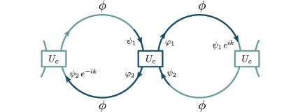
Figure 7: (Color online) Schematic of a 1D network model.

To begin, we consider the 1D network model shown in Fig. 7. At a typical node in the network, there is an input-output relation

$$\mathcal{U}_{c}\begin{pmatrix}\psi_{1}\\ \psi_{2}\end{pmatrix}=\begin{pmatrix}\varphi_{1}\\ \varphi_{2}\end{pmatrix},$$ (29)

where $\psi_{1}$, $\psi_{2}$, $\varphi_{1}$, and $\varphi_{2}$ are the complex wave amplitudes at the positions indicated in the figure, and $\mathcal{U}_{c}$ is a fixed $2\times 2$ unitary coupling matrix. For a Bloch state with quasimomentum $k$, the wave amplitudes are further related by $\varphi_{1}=e^{-i\phi}e^{ik}\psi_{1}$ and $\varphi_{2}=e^{-i\phi}\,e^{-ik}\psi_{2}$, where $\phi$ is the link delay. The $k$-space evolution matrix is

$$U(k)=e^{-ik\sigma_{z}}\,\mathcal{U}_{c}.$$ (30)

Note that $\mathcal{U}_{c}$ is independent of $k$. We can map $U(k)$ onto the evolution matrix for a DTQW for a particle in a 1D lattice, with internal “spin up” ($\uparrow$) and “spin down” ($\downarrow$) degrees of freedom. The DTQW is divided into two steps. In the first step, we apply $U_{c}$ on every lattice site. In the second step, we perform a spin-dependent translation that moves $\uparrow$ one site to the left, and $\downarrow$ one site to the right:

$$\sum_{j}|j-1\rangle\langle j|\otimes|\uparrow\;\rangle\langle\;\uparrow|+|j+1\rangle\langle j|\otimes|\downarrow\;\rangle\langle\;\downarrow|\\ =\int_{-\pi}^{\pi}dk\;e^{-ik\sigma_{z}}\otimes|k\rangle\langle k|\;.$$ (31)

Then, for each $k$, the evolution operator over one period of the DTQW reduces to Eq. (30).

We can similarly map our 3D network model to a 3D DTQW. Start from the scattering at a given node, which is described by the unitary scattering relation (15). To relate this to the quantum walk, observe that

$$\begin{aligned} \begin{pmatrix}e^{-ik_{\mu}}&0\\ 0&1\end{pmatrix}&=e^{-ik_{\mu}/2}e^{-ik_{\mu}\sigma_{z}/2}\\ \begin{pmatrix}1&0\\ 0&e^{ik_{\mu}}\end{pmatrix}&=e^{ik_{\mu}/2}e^{-ik_{\mu}\sigma_{z}/2}\\ \begin{pmatrix}\sin\theta_{\mu}&i\cos\theta_{\mu}\\ i\cos\theta_{\mu}&\sin\theta_{\mu}\end{pmatrix}&=e^{-i(\theta_{\mu}-\frac{\pi}{2})\sigma_{x}}.\end{aligned}$$ (32)

We can combine these operations to obtain

$$U_{\mu}=e^{-ik_{\mu}\sigma_{z}/2}e^{-i(\theta_{\mu}-\frac{\pi}{2})\sigma_{x}}e^{-ik_{\mu}\sigma_{z}/2},$$ (33)

where $U_{\mu}$ has the form given in (19). Hence, we can generate the Floquet evolution matrix $U=U_{z}U_{y}U_{x}$. The DQTW protocol thus consists of three steps, one for each direction $\{x,y,z\}$, where each step consists of two spin rotations and one spin-dependent translation along the chosen direction.

Other periodic network models with more complicated configurations can also be mapped onto DTQWs, but the mapping may require more than two internal degrees of freedom. Consider a periodic network of arbitrary dimension, where each unit cell contains an arbitrary configuration of coupling nodes, joined by links of equal phase delay $\phi$, with some of the links connecting to adjacent unit cells. As described in Ref. Yidong2014, , the whole set of node couplings in one unit cell can be described by

$$\mathcal{U}_{c}\,\vec{\psi}=\vec{\varphi},$$ (34)

where $\vec{\psi}=[\psi_{1},\dots,\psi_{N}]$ and $\vec{\varphi}=[\varphi_{1},\dots,\varphi_{N}]$ are vectors of wave amplitudes that are incoming and outgoing from the nodes, and $\mathcal{U}_{c}$ is an $N\times N$ unitary matrix. The $\vec{\psi}$ and $\vec{\varphi}$ vectors can always be arranged so that, for each $n$, $\varphi_{n}$ and $\psi_{n}$ lie on the opposite ends of equivalent links, either in the same unit cell or another unit cell (refer again to Fig. 7 for a 1D example). Then we can write

$$\vec{\varphi}=e^{-i\phi}\mathcal{D}(\vec{k})\,\vec{\psi},$$ (35)

where $\mathcal{D}(\vec{k})$ is a diagonal matrix where each diagonal element has the form $\exp(i\vec{k}\cdot\vec{d}_{n})$, and $\vec{d}_{n}$ is a lattice displacement vector representing the lattice displacement for link $n$. Hence, the periodic network can be described by a $k$-space unitary evolution matrix $U(k)=[\mathcal{D}(k)]^{-1}\,\mathcal{U}_{c}$. This can be implemented as a DTQW, with $[\mathcal{D}(k)]^{-1}$ realized using a translation operation analogous to Eq. (31).

References

- (1) X. Wan, A. M. Turner, A. Vishwanath, and S. Y. Savrasov, Phys. Rev. B83, 205101 (2011).
- (2) G. Xu, H. Weng, Z. Wang, X. Dai, and Z. Fang, Phys. Rev. Lett. 107, 186806 (2011).
- (3) L. Lu, L. Fu, J. D. Joannopoulos, et al. Nature photonics 7, 294 (2013).
- (4) H. Weyl, Z. Phys. 56, 330–352 (1929).
- (5) S. Y. Xu et al., Science 7, 613 (2015).
- (6) B. Q. Lv, H. M. Weng, B. B. Fu, X. P. Wang, H. Miao, J. Ma, P. Richard, X. C. Huang, L. X. Zhao, G. F. Chen, Z. Fang, X. Dai, T. Qian, H. Ding, Phys. Rev. X 5, 031013 (2015).
- (7) L. Lu, Z. Wang, D. Ye, L. Ran, L. Fu, J. D. Joannopoulos, and M. Soljacic, Science 7, 622 (2015).
- (8) M. Xiao, W. J. Chen, W. Y. He, et al. Nature Physics 11, 920 (2015).
- (9) S. M. Young, S. Zaheer, J. C. Y. Teo, C. L. Kane, E. J. Mele, and A. M. Rappe, Phys. Rev. Lett. 108, 140405 (2012).
- (10) Although we refer to “Fermi arcs”, in electromagnetic bandstructures the particles do not obey Fermi statistics.
- (11) J. I. Inoue and A. Tanaka, Phys. Rev. Lett. 105, 017401 (2010).
- (12) N. H. Lindner, G. Refael, and V. Galitski, Nature Physics 7, 490 (2011).
- (13) D. Y. H. Ho and J. B. Gong, Phys. Rev. Lett. 109, 010601 (2012).
- (14) T. Kitagawa, E. Berg, M. Rudner, and E. Demler, Phys. Rev. B82, 235114 (2010).
- (15) M. S. Rudner, N. H. Lindner, E. Berg, and M. Levin, Phys. Rev. X 3, 031005 (2013).
- (16) P. Titum, E. Berg, M. S. Rudner, G. Refael, and N. H. Lindner, arxiv:1506.00650.
- (17) D. Y. H. Ho and J. B. Gong, Phys. Rev. B90, 195419 (2014).
- (18) M. C. Rechtsman, J. M. Zeuner, Y. Plotnik, Y. Lumer, D. Podolsky, F. Dreisow, S. Nolte, M. Segev, and A. Szameit, Nature 496, 196 (2013).
- (19) G. Q. Liang and Y. D. Chong, Phys. Rev. Lett. 110, 203904 (2013).
- (20) G. Q. Liang and Y. D. Chong, Int. J. Mod. Phys. B 28, 1441007 (2014).
- (21) M. Pasek and Y. D. Chong, Phys. Rev. B89, 075113 (2014).
- (22) W. Hu, J. C. Pillay, K. Wu, M. Pasek, P. P. Shum, and Y. D. Chong, Phys. Rev. X 5, 011012 (2015).
- (23) F. Gao et al., arXiv:1504.07809.
- (24) G. Jotzu, M. Messer, R. Desbuquois, M. Lebrat, T. Uehlinger, D. Greif, And T. Esslinger, Nature 515, 237 (2014).
- (25) N. H. Lindner, D. L. Bergman, G. Refael, and V. Galitski, Phys. Rev. B 87, 235131 (2013).
- (26) R. Wang, B. Wang, R. Shen, L. Sheng and D. Y. Xing, Europhys. Lett. 105, 17004 (2014).
- (27) H. L. Calvo, L. E. F. Foa Torres, P. M. Perez-Piskunow, C. A. Balseiro, and G. Usaj, Phys. Rev. B 91, 241404 (2015).
- (28) A. Narayan, Phys. Rev. B 91, 205445 (2015).
- (29) R. W. Bomantara, G. N. Raghava, L. Zhou, and J. Gong, Phys. Rev. E 93, 022209 (2016).
- (30) J.-Y. Zhou and B.-G. Liu, arXiv:1601.04497.
- (31) J. T. Chalker and P. D. Coddington, J. Phys. C 21, 2665 (1988).
- (32) M. Hafezi, E. A. Demler, M. D. Lukin, and J. M. Taylor, Nat. Phys. 7, 907 (2011).
- (33) M. Hafezi, S. Mittal, J. Fan, A. Migdall, and J. M. Taylor, Nat. Photonics 7, 1001 (2013).
- (34) Z. Wang, Y. D. Chong, J. D. Joannopoulos, and M. Soljacic, Nature 461, 7265 (2009).
- (35) C. Tauber and P. Delplace, New J. Phys. 17, 115008 (2015).
- (36) S. Murakami, New J. Phys. 9, 356 (2007).
- (37) J. T. Chalker, and A. Dohmen, Phys. Rev. Lett. 75, 4496 (1995).
- (38) S. Murakami and S. I. Kuga, Phys. Rev. B78, 165313 (2008).
- (39) C.-M. Ho, and J. T. Chalker, Phys. Rev. B54, 8708 (1996).
- (40) P. Hosur, X. Qi, Comptes Rendus Physique 14, 857 (2013).
- (41) H. B. Nielsen, M. Ninomiya, Nuclear Physics B 185, 20 (1981).
- (42) H. B. Nielsen, M. Ninomiya, Nuclear Physics B 193, 173 (1981).
- (43) S. Ryu, A. P. Schnyder, A. Furusaki, and A. W. W. Ludwig, New J. Phys. 12, 065010 (2010).
- (44) A. A. Burkov, J. Phys.: Cond. Mat. 27, 113201 (2015).
- (45) J. E. Avron, R. Seiler, B. Simon, Phys. Rev. Lett. 51, 51 (1983).
- (46) J. E. Moore and L. Balents, Phys. Rev. B75,121306 (2007).
- (47) M. Z. Hasan and C. L. Kane, Rev. Mod. Phys. 82, 3045 (2010).
- (48) P. W. Brouwer, Phys. Rev. B58, R10135 (1998).
- (49) D. Meidan, T. Micklitz, and P. W. Brouwer, Phys. Rev. B 84, 195410 (2011).
- (50) I. C. Fulga, F. Hassler, and A. R. Akhmerov, Phys. Rev. B85, 165409 (2012).
- (51) I. C. Fulga and M. Maksymenko, arxiv:1508.02726.
- (52) L. Fu, C. L. Kane, and E. J. Mele, Phys. Rev. Lett. 98, 106803 (2007).
- (53) M. Karski, L. Frster, J. M. Choi, A. Steffen, W. Alt, D. Meschede, and A. Widera, Science 325, 174 (2009).
- (54) H. De Raedt, A. Lagendijk, and P. de Vries, Phys. Rev. Lett. 62, 47 (1989).