Non-local image deconvolution by Cauchy sequence
Abstract
Abstract: We present the deconvolution between two smooth function vectors as a Cauchy sequence of weight functions. From this we develop a Taylor series expansion of the convolution problem that leads to a non-local approximation for the deconvolution in terms of continuous function spaces. Optimisation of this form against a given measure of error produces a theoretically more exact algorithm. The discretization of this formulation provides a deconvolution iteration that deconvolves images quicker than the Richardson-Lucy algorithm.
Keywords: deconvolution, image processing, Banach spaces, Cauchy sequences, Richardson-Lucy
Introduction
The deconvolution of images is a frequent inverse problem occurring in scientific and engineering applications. In particular, problems involving smooth images and kernels in two or more dimensions are described by:
| (1) |
The objective, given and , is to find the image where is the observed image, is the function to be determined and is the convolving kernel. We explicitly assume in the following analysis that the images are differentiable and noiseless.
Given two continuous integrable images, and that are related by equation (1), it can be shown that there exists a continuous bijection on the complete Banach space of functions that will deconvolve from . Writing:
| (2) |
the solution can be written:
| (3) |
Equation (3) is the Von Neumann series from the general theory of linear operators [1, 3]. However, the convolution integral has additional mathematical structure that can be used to optimise the deconvolution beyond the general iterative process given in equation (3). The approach of this article is to determine an alternative convergent series for equation (1). Section 1 presents an alternative to equation (3). Section 2 develops the series given in section 1. In section 3 the iteration developed in section 2 is accelerated using an auxilliary Richardson-Lucy iteration. Section 4 develops a simple noise suppression strategy for the results of section 3. Section 5 numerically analyses these results by directly deconvolving a discrete test image. Section 6 concludes. Section 7 presents figures. Section 8 cites the most important references used in the development of this work.
1 Existence of an alternative parameterisation
From equation (3) derive a sequence of partial sums . Define the sequence of weight functions from equation (1):. Assuming that in equation (3) and are Cauchy sequences in the Banach space. Note in particular that for problems where is close to the identity operation, the th weight . Next we apply an important result to the sequence :
Lemma 1 The convergent sequence of sums is not unique. Proof: The sequence is by definition absolutely convergent. Therefore the series of some subsequence of is also convergent and rearrangable. Writing generates an arbitrary subsequence of which proves the lemma.
| (5) |
where:
| (6) |
The sequence where is an alternative to the Von Neumann series for , where both and are equal to the solution . In the next section we derive an explicit form for equation (5).
2 Explicit form for an alternative sequence
Given equation (5) note the well known property of convolution integrals, . Together with we have . Expanding about :
| (7) |
| (8) |
where we define the following operator symbols for :
so that , and . The scalar product operator is represented as a vector integral operation on the nabla, . Noting that the antisymmetric moments [8] for together with Stirling’s approximation for leads to a direct representation of the convolution in terms of the weight functions and :
| (9) |
where . The inequality becomes an equality in the limit . The integral moment ratios in equation (9) vary slowly over and in particular for symmetric kernels we have . Using these facts in equation (9) gives :
If the terms of the rightmost sum in equation (9) are negligible beyond then:
| (10) |
represents the convolution well for a fixed value. Inverting this relationship estimates the deconvolution :
| (11) |
By definition:
| (12) |
which implies the approximate iteration formula:
| (13) |
The inverted convolution sequence is bounded by the exponential series in equation (9) and is therefore Cauchy, since equation (12) . Further, since equation (13) considers all the moments in equation (9) to be equal, it appears to be local in the sense of [8]: note however that the division of by in equation (13) negates such a comparision.
The leftmost sum of equation (9) would be better reproduced by iteration (13) when is considered to be an unknown function of , since iteration (13) is an upper bound approximation to the correct sequence . Therefore, given that the convolution problem is not specified by a unique Cauchy sequence (lemma 1), equation (13) can be made optimal relative to some measure of error if we write:
| (14) |
3 Auxilliary acceleration
For large , to a good approximation, we have substitution for on the left hand side of this expression leads to the well known Richardson-Lucy [4] propagator for :
| (15) |
| (16) |
4 Noise suppression
Equation (15) is recognisable as the th iteration of the Richardson-Lucy algorithm without the accompanying right convolution with . Therefore it is prudent to modify equation (15):
| (17) |
Using this in equation (14):
| (18) |
Starting the algorithm with an initial value will generate a nabla term acting on every that generates noise in the solution at every iteration. This build up of noise is proportional to and destroys the convergence properties of the algorithm beyond a certain number of iterations.
The noise statistics of a differential operator exhibit a “random walk” phenomenon in its function space without any overall cancellation in the noise. After a sufficient number of iterations the norm of the derivative is characterised just by the noise function and, . Therefore iteration (18) is no longer representative of the exponential operator series (13) when noise is present, rather the operator diverges as for large values of . It is therefore prudent to normalise the derivative .
This strategy gives good noise suppression as intended, which suggests that the power of in the denominator can be tuned just enough to correct for derivative noise and at the same time optimise the signal propagator so that overall the algorithm converges correctly according to equation (14). Using these developments in equation (18) gives the following iteration for a 2 dimensional image convolved by a symmetric kernel :
| (19) |
where and need to be determined per iteration in order that convergence is optimised - see equation (20).
5 Results and observations
All results are computed with MATLAB© and the algorithm is implemented in discrete form by modifying the MATLAB© “deconvlucy” command in accordance with equation (19) multiplied through by . All norms are taken as root mean square (RMS) values.
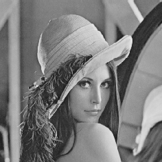
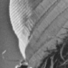
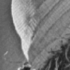
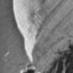
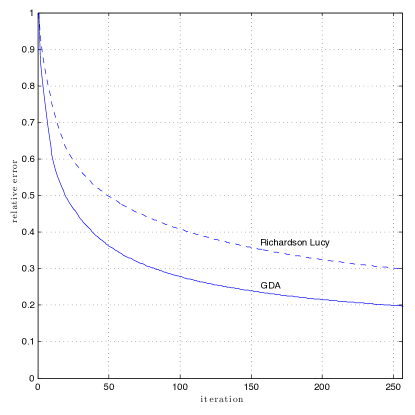
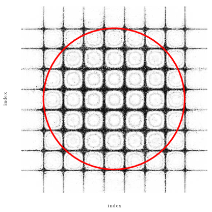
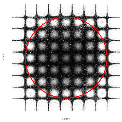
To demonstrate the approach we convolve a noiseless, greyscale, “Lena” image matrix, , by a Gaussian radial kernel of standard deviation 5 pixels clipped at 9 pixels and then reverse the process by using equation (19). We also take the same blurred image and deblur using the original MATLAB© “deconvlucy” command and compare the obtained relative error in the two approaches. The results are given in figures 1 and 3. These show the original image followed by the approximations obtained after 256 iterations of each algorithm. In each case visual convergence is good. However upon closer inspection it can be seen that equation (19) recovers the ridge detail of Lena’s hat per iteration better than the Richardson-Lucy algorithm.
Analysing the relative error, , it is clear that for this kind of image the present algorithm performs better. The form of iteration (14) guarantees this because it, when inverted, tends to reproduce the entire leftmost series expansion (9) for .
Regularisation of the measured image gives an estimate for the relative error function:
| (20) |
The norm of this expression can be minimised at every iteration, to generate an optimal set for equation (14). Equation (14) is then made optimal to the th order with respect to equation (9) in the sense of the Cauchy sequence where is the minimum error.
We remark that the running optimisation procedure for is still the subject of ongoing research. The results presented in this paper are for constant values.
Taking Fourier transforms of the approximate series (11) [5] leads to an expression for the Fourier transform in terms of the Fourier transform of :
| (21) |
which demonstrates that the operator series (11) effectively regularises the sequence starting point by an exponential upper bound. Referring to iteration (13), the amount of exponential regularisation applied to the Cauchy sequence is directly controlled by the convolution moments of the image in frequency space. Equation (21) shows that the impact on the overall “reach” of the algorithm into frequency space of the weight functions is characterised by:
| (22) |
By itself, there is nothing new in an exponential regularisation, it is already well known. The difference here is in how it arises from Cauchy sequences, is used in equation (19) and what it actually influences in the sequence. These features may make the approach useful from both a theoretical as well as practical standpoint.
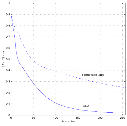
For this reason we also add another test measure, based on the norm of the ratio of the Fourier transforms (FTR) of each image, where is proportional to for large .
From a practical point of view, this is is perhaps the most important number since a value of the FTR indicates that the deconvolution algorithm is inefficient at recovering high frequency detail effectively and acts like a low pass filter. For the theory of this paper, the low pass filter interpretation is supported by the implication of a small value for and consequently a large value for which would tend to invalidate equation (10). In that situation the optimised form of the iteration would then be required to make further progress.
If instead the FTR for a recovered image then the chances are that fine details in the image have been recovered well and the algorithm consequently has good reach into the high frequency components of the Fourier space. Theoretically, this implies that be large and the value consequently small. In this situation the exponential series (10) represents the deconvolution well.
6 Conclusions
The algorithm presented derives the deconvolution operator for images as a possible Cauchy sequence of weight functions in the space of solution images. The initial results verify that there is indeed a measurable advantage to be had in this adopting this approach.
The results here have been deliberately restricted to Cauchy sequences using symmetric kernels, but in principle the equations can be potentially extended to different types of kernel through the use of equation (9).
Furthermore, according to lemma 1, the Cauchy sequence demonstrated in equation (14) is not necessarily unique. It can be shown that a more general , exact form of equation (5) or (11) is:
| (23) |
which can be used if an operator form for is available.
Among the advantages associated with techniques that use convergent sequences like equation (4) is that problems like dimensionality, mathematical representation and the question of continuous or discrete data spaces, become technical issues. Instead, an appreciation of the concepts of convergence and accuracy and their impact on the quality of the image reconstruction become central to the discussion.
This has happened before with the Richardson-Lucy algorithm which subsequently has found a wide range of application everywhere. Specialising the image to a two dimensional series we were able to derive an improved two-step, non-local version of it for this paper, which may be used as a simple but promising alternative.
A related fact is that since deconvolution problems occur frequently, not just in image processing, but are in fact very common to every area of physics and engineering, a closed form series like equation (11) and more generally (23) can potentially be of use in problems such as viscoelasticity, diffraction and quantum mechanics to name but a few other areas of potential application.
From a purely theoretical perspective, the technique of finding an approximate closed form Cauchy deconvolution sequence in direct space mimics the natural one in Fourier space: The Fourier transform of is the ratio of the Fourier transform of and . This commodity is what in principal makes that approach appealing: the formal “rotation” of the problem into Fourier space simplifies it. The iterative summing of the Cauchy sequence as in equation (14) or when applicable (11), provides just such an analogue in direct space once has been found.
7 Figures


8 Bibliography
References
- [1] Halsey G., Blass W. E., “Deconvolution of IR spectra in real time”, Applied Optics, 1977
- [2] Cameron D. H., Kauppinen J. K., Moffatt D. J., Mantsch H. H., “Precision in Condensed Phase Vibrational Spectroscopy”, Applied Spectroscopy, Volume 36, Number 3, 1982v
- [3] Jones A. F., Misell D. L., “The problem of error in deconvolution”,J. Phys. A: Gen. Phys. 3 462, 1970
- [4] Jones R. N., Shimokoshi K., “Some observations on the resolution enhancement of spectral data by the method of self-deconvolution”, Applied Spectroscopy, Volume 37, Number 1, 1983
- [5] Kauppinen J. K., Moffatt D. J., Mantsch H. H., Cameron D. G., “Fourier Transforms in the Computation of Self-Deconvoluted and First-Order Derivative Spectra of Overlapped Band Contours”, American Chemical Society, Anal. Chem. 1981, 53, 1454-1457, 1981
- [6] Shimokoshi K., Kanzaki T., Jones R. N., “Deconvolution of Mossbauer Spectra by the Finite Impulse Response Operator (FIRO) Method”, Applied Spectroscopy, Volume 39, Number 6, 1985
- [7] Shimokoshi K., Jones R. N., “The Resolution Enhancement of Electron Spin Resonance Spectra by Self-deconvolution with a Finite Impulse Response Operator”, Applied Spectroscopy, Volume 37, Number 1, 1983
- [8] Gureyev T. E., Nesterets Y. I., Stevenson A. W., Wilkins S. W., “A method for local deconvolution”, Applied Optics, Vol. 42, No. 32, 10 November 2003
- [9] Lathawer L. D., de Baynast A., “Blind Deconvolution of DS-CDMA Signals by Means of Decomposition in Rank- (1 ; L; L ) Terms”, IEEE Transactions on Signal Processing, Vol. 56, no. 4, April 2008
- [10] Prost R., Gouette R., “Deconvolution When the Convolution Kernel Has No Inverse”, IEEE Transactions on Acoustics, Speech and Signal Processing, Vol. ASSP-25, no. 6 , December 1977
- [11] Raina R. K., Koul C. L., “On convolution of Integral Equations”, Indian J. pure appl Math., 13(3): 362-369, March 1982