Universality Laws for Randomized Dimension Reduction,
with Applications

Abstract.

Dimension reduction is the process of embedding high-dimensional data into a lower dimensional space to facilitate its analysis. In the Euclidean setting, one fundamental technique for dimension reduction is to apply a random linear map to the data. This dimension reduction procedure succeeds when it preserves certain geometric features of the set. The question is how large the embedding dimension must be to ensure that randomized dimension reduction succeeds with high probability.

This paper studies a natural family of randomized dimension reduction maps and a large class of data sets. It proves that there is a phase transition in the success probability of the dimension reduction map as the embedding dimension increases. For a given data set, the location of the phase transition is the same for all maps in this family. Furthermore, each map has the same stability properties, as quantified through the restricted minimum singular value. These results can be viewed as new universality laws in high-dimensional stochastic geometry.

Universality laws for randomized dimension reduction have many applications in applied mathematics, signal processing, and statistics. They yield design principles for numerical linear algebra algorithms, for compressed sensing measurement ensembles, and for random linear codes. Furthermore, these results have implications for the performance of statistical estimation methods under a large class of random experimental designs.

1. Overview of the Universality Phenomenon

This paper concerns a fundamental question in high-dimensional stochastic geometry:

1. Is it likely that a random subspace of fixed dimension does not intersect a given set?

This problem has its roots in the earliest research on spherical integral geometry [San52, San76], and it also arises in asymptotic convex geometry [Gor88]. In recent years, this question has attracted fresh attention [Don06c, RV08, Sto09, DT09b, CRPW12, ALMT14, Sto13, MT13, OH13, OTH13, TOH15, TAH15] because it is central to the analysis of randomized dimension reduction.

This paper establishes that a striking universality phenomenon takes place in the stochastic geometry problem (Q1). For a given set, the answer to this question is essentially the same for every distribution on random subspaces that is induced by a natural model for random linear maps. Universality also manifests itself in metric variants of (Q1), where we ask how far the random subspace lies from the set. We discuss the implications of these results in high-dimensional geometry, random matrix theory, numerical analysis, optimization, statistics, signal processing, and beyond.

1.1. Randomized Dimension Reduction

Dimension reduction is the operation of mapping a set from a large space into a smaller space. Ideally, this action distills the “information” in the set, and it allows us to develop more efficient algorithms for processing that information. In the setting of Euclidean spaces, a fundamental method for dimension reduction is to apply a random linear map to each point in the set. It is important that the random linear map preserve geometric features of the set. In particular, we do not want the linear map to map a point in the set to the origin. Equivalently, the null space of the random linear map should not intersect the set. We see that (Q1) emerges naturally in the context of randomized dimension reduction.

1.2. Technical Setting

Let us introduce a framework in which to study this problem. It is natural to treat (Q1) as a question in spherical geometry because it is scale invariant. Fix the ambient dimension $D$, and consider a closed subset $\Omega$ of the Euclidean unit sphere in $\mathbb{R}^{D}$. For the moment, we also assume that $\Omega$ is spherically convex; that is, $\Omega$ is the intersection of a convex cone with the unit sphere. Construct a random linear map $\bm{\Pi}:\mathbb{R}^{D}\to\mathbb{R}^{d}$, where the embedding dimension $d$ does not exceed the ambient dimension $D$. As we vary the distribution of the random linear map $\bm{\Pi}$, the map $\bm{\Pi}\mapsto\operatorname{null}(\bm{\Pi})$ induces different distributions on the subspaces in $\mathbb{R}^{D}$ with codimension at most $d$. We may now reformulate (Q1) in this language:

1. For a given embedding dimension $d$, what is the probability that $\Omega\cap\operatorname{null}(\bm{\Pi})=\emptyset$? Equivalently, what is the probability that $\bm{0}\notin\bm{\Pi}(\Omega)$?

We say that the random projection succeeds when $\bm{0}\notin\bm{\Pi}(\Omega)$. Conversely, when $\bm{0}\in\bm{\Pi}(\Omega)$, we say that the random projection fails. See Figure 1.1 for an illustration.

We have the intuition that, for a fixed choice of $\Omega$, the projection is more likely to succeed as the embedding dimension $d$ increases. Furthermore, a random linear map $\bm{\Pi}$ with fixed embedding dimension $d$ is less likely to succeed as the size of the set increases. We will justify these heuristics in complete detail.

Figure 1.1. Geometry of a Random Linear Map. We can identify a linear map $\bm{\Pi}:\mathbb{R}^{D}\to\mathbb{R}^{d}$ with an orthogonal projector $\bm{P}:\mathbb{R}^{D}\to\mathbb{R}^{D}$ whose range is the orthogonal complement of $\operatorname{null}(\bm{\Pi})$. In this diagram, $\bm{P}:\mathbb{R}^{2}\to\mathbb{R}^{2}$ is a random orthogonal projector applied to a closed, spherically convex set $\Omega$. The likelihood of a given configuration depends on the statistical dimension $\delta(\Omega)$ of the set. Left: Success Regime. The null space, $\operatorname{null}(\bm{P})$, does not intersect $\Omega$, and the image $\bm{P}(\Omega)$ does not contain the origin. Right: Failure Regime. The null space, $\operatorname{null}(\bm{P})$, intersects the set $\Omega$, and the image $\bm{P}(\Omega)$ contains the origin.

1.3. A Phase Transition for Uniformly Random Partial Isometries

We begin with a case where the literature already contains a comprehensive answer to the question (Q2).

The most natural type of random embedding is a uniformly random partial isometry. That is, $\bm{\Pi}:\mathbb{R}^{D}\to\mathbb{R}^{d}$ is a partial isometry whose null space, $\operatorname{null}(\bm{\Pi})$, is drawn uniformly at random from the Haar measure on the Grassmann manifold of subspaces in $\mathbb{R}^{D}$ with codimension $d$. The invariance properties of the distribution of $\bm{\Pi}$ allow for a complete analysis of its action on $\Omega$, the spherically convex set [SW08, Chap. 6.5]. Recent research [ALMT14, MT14a, GNP14] has shown how to convert the complicated exact formulas into interpretable results.

The modern theory is expressed in terms of a geometric functional $\delta(\Omega)$, called the statistical dimension:

$$\delta(\Omega):=\operatorname{\mathbb{E}}\left[\left(\max_{\bm{t}\in\Omega}\bm{g}\cdot\bm{t}\right)_{+}^{2}\right],\quad\text{where $\bm{g}$ is $\textsc{normal}(\bm{0},\mathbf{I})$.}$$

The statistical dimension is increasing with respect to set inclusion, and its values range from zero (for the empty set) up to $D$ (for the whole sphere). Furthermore, the functional can be computed accurately in many cases of interest. See Section 3.3 for more details.

The statistical dimension demarcates a phase transition in the behavior of a uniformly random partial isometry $\bm{\Pi}$ as the embedding dimension $d$ varies. For a closed, spherically convex set $\Omega$, the results [ALMT14, Thm. I and Prop. 10.2] demonstrate that

$$d \leq\delta(\Omega)-\mathrm{C}\sqrt{\delta(\Omega)}\quad\text{implies}\quad\bm{0}\in\bm{\Pi}(\Omega)\quad\text{with high probability};$$ (1.1)

$$d \geq\delta(\Omega)+\mathrm{C}\sqrt{\delta(\Omega)}\quad\text{implies}\quad\bm{0}\notin\bm{\Pi}(\Omega)\quad\text{with high probability}.$$

The number $\mathrm{C}$ is a positive universal constant. In other terms, a uniformly random projection $\bm{\Pi}(\Omega)$ of a spherically convex set $\Omega$ is likely to succeed precisely when the embedding dimension $d$ is larger than the statistical dimension $\delta(\Omega)$. See Figure 1.2 for a plot of the exact probability that a uniformly random partial isometry annihilates a point in a specific set $\Omega$.

Remark 1.1 (Related Work).

The results [ALMT14, Thm. 7.1] and [MT13, Thm. A] contain good bounds for the probabilities in (1.1). The probabilities can be approximated more precisely by introducing a second geometric functional [GNP14]. These estimates depend on the spherical Crofton formula [SW08, Eqns. (6.62), (6.63)], which gives the exact probabilities in a less interpretable form. Related phase transition results can also be obtained via the Gaussian Minimax Theorem; see [Gor88, Cor. 3.4],  [ALMT14, Rem. 2.9], [Sto13], or [TOH15, Thm. II.1]. See [TH15] for other results on uniformly random partial isometries.

1.4. Other Types of Random Linear Maps?

The research outlined in Section 1.3 delivers a complete account of how a uniformly random partial isometry behaves in the presence of some convexity. In contrast, the literature contains almost no precise information about the behavior of other random linear maps.

Nevertheless, in applications, we may prefer—or be forced—to work with other types of random linear maps. Here is a motivating example. Many algorithms for numerical linear algebra now depend on randomized dimension reduction. In this context, uniformly random partial isometries are expensive to construct, to store, and to perform arithmetic with. It is more appealing to implement a random linear map that is discrete, or sparse, or structured. The lack of detailed theoretical information about how these linear maps behave makes it difficult to design numerical methods with guaranteed performance.

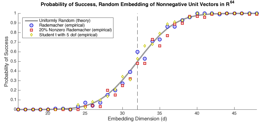
Figure 1.2. Universality of the Embedding Dimension. This plot describes the behavior of four types of random linear maps applied to the set $\Omega$ of unit vectors with nonnegative coordinates: $\Omega:=\{\bm{t}\in\mathbb{R}^{64}:\left\|{\bm{t}}\right\|=1,t_{i}\geq 0\}$. The dashed line marks the statistical dimension of the set: $\delta(\Omega)=32$. The gray curve interpolates the exact probability that a uniformly random partial isometry $\bm{\Pi}:\mathbb{R}^{64}\to\mathbb{R}^{d}$ succeeds (i.e., $\bm{0}\notin\bm{\Pi}(\Omega)$) as a function of the embedding dimension $d$. The markers indicate the empirical probability (over 100 trials) that dimension reduction succeeds for a random linear map with the specified distribution. See Sections 1.4 and 1.9 for further details.

We can, however, use computation to investigate the behavior of other types of random linear maps. Figure 1.2 presents the results of the following experiment. Consider the set $\Omega$ of unit vectors in $\mathbb{R}^{64}$ with nonnegative coordinates:

$$\Omega:=\big{\{}\bm{t}\in\mathbb{R}^{64}:\left\|{\bm{t}}\right\|=1\text{ and }t_{i}\geq 0\text{ for $i=1,\dots,64$}\big{\}}.$$

According to (3.6), below, the statistical dimension $\delta(\Omega)=32$, so the formula (1.1) tells us to expect a phase transition in the behavior of a uniformly random partial isometry when the embedding dimension $d=32$. Using [ALMT14, Ex. 5.3 and Eqn. (5.10)], we can compute the exact probability that a uniformly random partial isometry $\bm{\Pi}:\mathbb{R}^{64}\to\mathbb{R}^{d}$ succeeds as a function of $d$. Against this baseline, we compare the empirical probability (over 100 trials) that a random linear map with independent Rademacher entries succeeds. We also display experiments for a 20% nonzero Rademacher linear map and for a linear map with Student $t_{5}$ entries. See Section 1.9 for more details.

From this experiment, we discover that all three linear maps act almost exactly the same way as a uniformly random partial isometry! This universality phenomenon is remarkable because the four linear maps have rather different distributions. At present, the literature contains no information about when—or why—this phenomenon occurs.

1.5. A Universality Law for the Embedding Dimension

The central goal of this paper is to show that there is a substantial class of random linear maps for which the phase transition in the embedding dimension is universal. Here is a rough statement of the main result.

Let $\Omega$ be a closed, spherically convex set in $\mathbb{R}^{D}$. Suppose that the entries of the matrix of the random linear map $\bm{\Pi}:\mathbb{R}^{D}\to\mathbb{R}^{d}$ are independent, standardized, and symmetric, with a modest amount of regularity. In particular, we may consider random linear maps that have an arbitrarily small, but constant, proportion of nonzero entries. For this class of random linear maps, we will demonstrate that

$$d \leq\delta(\Omega)-o(D)\quad\text{implies}\quad\bm{0}\in\bm{\Pi}(\Omega)\quad\text{with high probability};$$ (1.2)

$$d \geq\delta(\Omega)+o(D)\quad\text{implies}\quad\bm{0}\notin\bm{\Pi}(\Omega)\quad\text{with high probability}.$$

The little-o notation suppresses constants that depend only on the regularity of the random variables that populate $\bm{\Pi}$. See Theorem I in Section 3.4 for a more complete statement.

The result (1.2) states that a random linear map $\bm{\Pi}$ is likely to succeed for a spherically convex set $\Omega$ precisely when the embedding dimension $d$ exceeds the statistical dimension $\delta(\Omega)$ of the set. We learn that the phase transition in the embedding dimension is universal over our class of random linear maps, provided that $\Omega$ is not too small as compared with the ambient dimension $D$. Note that a random linear map $\bm{\Gamma}:\mathbb{R}^{D}\to\mathbb{R}^{d}$ with standard normal entries has the same behavior as a $d\times D$ uniformly random partial isometry because, almost surely, the null space of $\bm{\Gamma}$ is a uniformly random subspace of $\mathbb{R}^{D}$ with codimension $d$. This analysis explains the dominant features of the experiment in Figure 1.2!

Figure 1.3. Geometry of the Restricted Minimum Singular Value. We can identify a partial unitary linear map $\bm{\Pi}:\mathbb{R}^{D}\to\mathbb{R}^{d}$ with an orthogonal projector $\bm{P}:\mathbb{R}^{D}\to\mathbb{R}^{D}$ whose range is the orthogonal complement of $\operatorname{null}(\bm{\Pi})$. In this diagram, $\bm{P}:\mathbb{R}^{2}\to\mathbb{R}^{2}$ is an orthogonal projector applied to a compact convex set $E$. The restricted minimum singular value $\sigma_{\min}(\bm{P};E)$ is the distance from the origin to the image $\bm{P}(E)$.

1.6. A Universality Law for the Restricted Minimum Singular Value

It is also a matter of significant interest to understand the stability of randomized dimension reduction. We quantify the stability of the random linear map $\bm{\Pi}:\mathbb{R}^{D}\to\mathbb{R}^{d}$ on a compact, convex set $E$ in $\mathbb{R}^{D}$ using the restricted minimum singular value:

$$\sigma_{\min}(\bm{\Pi};E):=\min_{\bm{t}\in E}\left\|{\bm{\Pi}\bm{t}}\right\|.$$

When the restricted minimum singular value $\sigma_{\min}(\bm{\Pi};E)$ is large, the random image $\bm{\Pi}(E)$ is far from the origin, so the embedding is very stable. That is, we can deform either the linear map $\bm{\Pi}$ or the set $E$ and still be sure that the embedding succeeds. When the restricted minimum singular value is small, the random dimension reduction map is unstable. When it is zero, the random dimension reduction map fails. See Figure 1.3 for a diagram.

Our second major theorem is a universality law for the restricted minimum singular values of a random linear map. This result is expressed using a geometric functional $\mathscr{E}_{d}(E)$, called the $d$-excess width of $E$:

$$\mathscr{E}_{d}(E):=\operatorname{\mathbb{E}}\min_{\bm{t}\in E}\big{(}\sqrt{d}\left\|{\bm{t}}\right\|+\bm{g}\cdot\bm{t}\big{)},\quad\text{where $\bm{g}$ is $\textsc{normal}(\bm{0},\mathbf{I})$.}$$

The $d$-excess width increases with the parameter $d$, and it decreases with respect to set inclusion. The typical scale of $\mathscr{E}_{d}(E)$ is $O(\sqrt{d})$. In addition, the excess width can be evaluated precisely in many situations of interest. See Section 4.2 for more details.

Now, suppose that the entries of the matrix of $\bm{\Pi}:\mathbb{R}^{D}\to\mathbb{R}^{d}$ are independent, standardized, and symmetric, with a modest amount of regularity. For a compact, convex subset $E$ of the unit ball in $\mathbb{R}^{D}$, we will establish that

$$\sigma_{\min}(\bm{\Pi};E)=\big{(}\mathscr{E}_{d}(E)\big{)}_{+}+o(\sqrt{d})\quad\text{with high probability.}$$ (1.3)

The little-o notation suppresses constants that depend only on the regularity of the random variables. Theorem II in Section 4.3 contains a more detailed statement of (1.3).

In summary, provided that the set $E$ is not too small, the restricted minimum singular value $\sigma_{\min}(\bm{\Pi};E)$ depends primarily on the geometry of the set $E$ and the embedding dimension $d$, rather than on the distribution of the random linear map $\bm{\Pi}$. See Figure 1.4 for a numerical illustration of this fact.

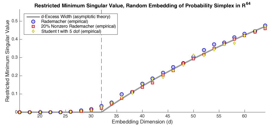
Figure 1.4. Universality of the Restricted Minimum Singular Value. This plot describes the behavior of three types of random linear maps applied to the probability simplex $\Delta_{64}:=\{\bm{t}\in\mathbb{R}^{64}:\sum_{i}t_{i}=1,t_{i}\geq 0\}$. The dashed line marks the minimum dimension $d=32$ where uniformly random embedding of the set $\Delta_{64}$ is likely to succeed. The gray curve interpolates the value of the positive part $\big{(}\mathscr{E}_{d}(\Delta_{64})\big{)}_{+}$ of the $d$-excess width of $\Delta_{64}$, obtained from the asymptotic calculation (4.4). The markers give an empirical estimate (over 100 trials) for the restricted minimum singular value $\sigma_{\min}(\bm{\Pi};\Delta_{64})$ of a random linear map $\bm{\Pi}:\mathbb{R}^{64}\to\mathbb{R}^{d}$ drawn from the specified distribution. See Section 1.9 for more information.

1.7. Applications of Universality

Randomized dimension reduction and, more generally, random matrices have become ubiquitous in the information sciences. As a consequence, the universality laws that we outlined in Section 1.5 and 1.6 have a wide range of implications.

Signal Processing:

The main idea in the field of compressed sensing is that we can acquire information about a structured signal by taking random linear measurements. The literature contains extensive empirical evidence that many types of random measurements behave in an indistinguishable fashion. Our work gives the first explanation of this phenomenon. (Section 5)

Stochastic Geometry:

Our results also indicate that the facial structure of the convex hull of independent random vectors, drawn from an appropriate class, does not depend heavily on the distribution. (Section 5.3.1)

Coding Theory:

Random linear codes provide an efficient way to protect transmissions against error. We demonstrate that a class of random codes is resilient against sparse corruptions. The number of errors that can be corrected does not depend on the specific choice of codebook. (Section 6)

Numerical Analysis:

Our research provides an engineering design principle for numerical algorithms based on randomized dimension reduction. We can select the random linear map that is most favorable for implementation and still be confident about the detailed behavior of the algorithm. This approach allows us to develop efficient numerical methods that also have rigorous performance guarantees. (Section 7)

Random Matrix Theory:

Our work leads to a new proof of the Bai–Yin law for the minimum singular value of a random matrix with independent entries. (Section 7.1)

High-Dimensional Statistics:

The LASSO is a widely used method for performing regression and variable selection. We demonstrate that the prediction error associated with a LASSO estimator is universal across a large class of random designs and statistical error models. We also show that least-absolute-deviation (LAD) regression can correct a small number of arbitrary statistical errors for a wide class of random designs. (Section 8 and Remark 6.2)

Neuroscience:

Our universality laws may even have broader scientific significance. It has been conjectured, with some experimental evidence, that the brain may use dimension reduction to compress information [GG15]. Our universality laws suggest that many types of uncoordinated (i.e., random) activity lead to dimension reduction methods with the same behavior. This result indicates that the hypothesis of neural dimensionality reduction may be biologically plausible.

1.8. The Scope of the Universality Phenomenon

The universality phenomenon developed in this paper extends beyond the results that we establish, but there are some (apparently) related problems where universality does not hold. Let us say a few words about these examples and non-examples.

First, it does not appear important that the random linear map $\bm{\Pi}$ has independent entries. There is extensive evidence that structured random linear maps also have some universality properties; for example, see [DT09a].

Second, the restricted minimum singular value is not the only type of functional where universality is visible. For instance, suppose that $f$ is a convex, Lipschitz function. Consider the quantity

$$\min_{\bm{t}\in E}\big{(}\left\|{\bm{\Pi}\bm{t}}\right\|^{2}+f(\bm{t})\big{)}.$$

Optimization problems of this form play a central role in contemporary statistics and machine learning. It is likely that the value of this optimization problem is universal over a wide class of random linear maps. Furthermore, we believe that our techniques can be adapted to address this question. On the other hand, geometric functionals involving non-Euclidean norms need not exhibit universality. Consider the $\ell_{1}$ restricted minimum singular value

$$\min_{\bm{t}\in E}\left\|{\bm{\Pi}\bm{t}}\right\|_{\ell_{1}}.$$ (1.4)

There are nontrivial sets $E$ where the value of the optimization problem (1.4) varies a lot with the choice of the random linear map $\bm{\Pi}$. For instance, let $\mathbf{e}_{1}\in\mathbb{R}^{D}$ be the first standard basis vector, and define the shifted Euclidean ball

$$E_{\alpha}:=\big{\{}\bm{t}\in\mathbb{R}^{D}:\left\|{\bm{t}-\mathbf{e}_{1}}\right\|\leq\alpha\big{\}}\quad\text{for $0\leq\alpha\leq 1$.}$$

Using Theorem I and the calculation [ALMT14, Sec. 3.4] of the statistical dimension of a circular cone, we can verify that there is a universal phase transition for successful embedding of the set $E_{\alpha}$ when the embedding dimension $d=\alpha^{2}D+O(1)$. The result (1.3) implies that the minimum restricted singular value of $E_{\alpha}$ also takes a universal value. At the same time, Figure 1.5 illustrates that the functional (1.4) is not universal for the set $E_{\alpha}$.

Finally, functionals involving maximization do not necessarily exhibit universality. The restricted maximum singular value is defined as

$$\sigma_{\max}(\bm{\Pi};E):=\max_{\bm{t}\in E}\left\|{\bm{\Pi}\bm{t}}\right\|.$$

It is not hard to produce examples where the restricted maximum singular value depends on the choice of the random matrix $\bm{\Pi}$. For instance, Figure 1.6 demonstrates that the random linear map $\bm{\Pi}$ has a substantial impact on the maximum singular value $\sigma_{\max}(\bm{\Pi};\Delta_{D})$ restricted to the probability simplex $\Delta_{D}$ in $\mathbb{R}^{D}$. This observation may surprise researchers in random matrix theory because the ordinary maximum singular value is universal over the class of random matrices with independent entries [BS10, Thm. 3.10].

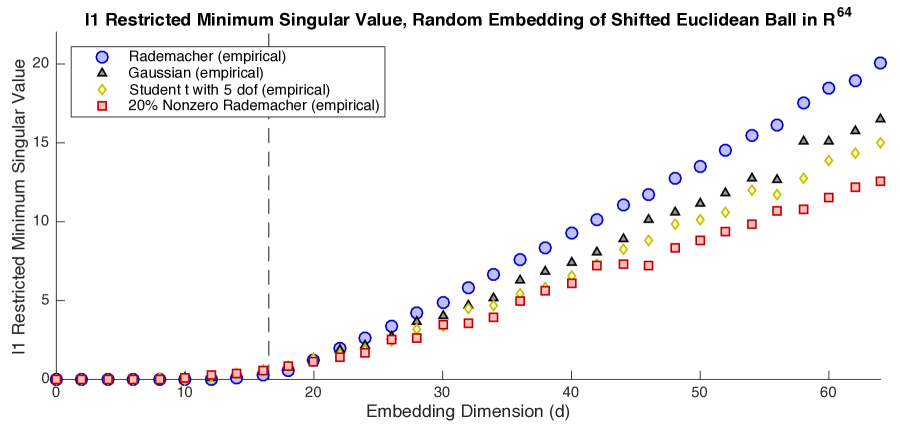
Figure 1.5. Non-Universality of the $\ell_{1}$ Restricted Minimum Singular Value. This plot describes the behavior of four types of random linear maps applied to the set $E_{1/2}:=\{\bm{t}\in\mathbb{R}^{64}:\left\|{\bm{t}-\mathbf{e}_{1}}\right\|\leq 1/2\}$, where $\mathbf{e}_{1}$ is the first standard basis vector. The dashed line stands at the phase transition $d\approx 16$ for the embedding dimension of the set $E_{1/2}$. The markers give an empirical estimate (over 100 trials) for the $\ell_{1}$ restricted minimum singular value $\min_{\bm{t}\in E_{1/2}}\left\|{\bm{\Pi}\bm{t}}\right\|_{\ell_{1}}$ of a random linear map $\bm{\Pi}:\mathbb{R}^{64}\to\mathbb{R}^{d}$ with the specified distribution as a function of the embedding dimension $d$. See Section 1.9 for more details.

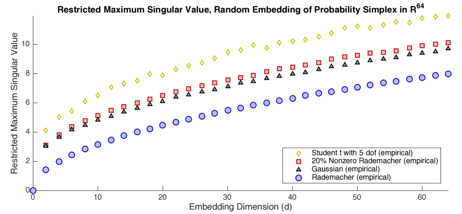
Figure 1.6. Non-Universality of the Restricted Maximum Singular Value. This plot describes the behavior of four types of random linear maps applied to the probability simplex $\Delta_{64}:=\{\bm{t}\in\mathbb{R}^{64}:\sum_{i}t_{i}=1,t_{i}\geq 0\}$. The markers give an empirical estimate (over 100 trials) for the restricted maximum singular value $\sigma_{\max}(\bm{\Pi};\Delta_{64})$ of a random linear map $\bm{\Pi}:\mathbb{R}^{64}\to\mathbb{R}^{d}$ with the specified distribution. See Section 1.9 for more details.

1.9. Reproducible Research

This paper is accompanied by MATLAB code [Tro15a] that reproduces each figure from stored data. This software can also repeat the numerical experiments to obtain new instances of each figure. By modifying the parameters in the code, the reader may explore how changes affect the universality phenomenon. We omit meticulous descriptions of the numerical experiments from the text because these recitations are tiresome for the reader and the code offers superior documentation.

1.10. Roadmap

This paper is divided into five parts. Part I offers a complete presentation of our universality laws, some comments about the proofs, and some prospects for further research. Part II outlines the applications of universality in several disciplines, and it contains more empirical confirmation of our analysis. Part III presents the proof that the restricted minimum singular value exhibits universal behavior; this argument also yields the condition in which randomized embedding is likely to succeed. Part IV contains the proof of the condition in which randomized embedding is likely to fail. Finally, Part V includes background results, the acknowledgments, and the list of works cited.

1.11. Notation

Let us summarize our notation. We use italic lowercase letters (for example, $a$) for scalars, boldface lowercase letters ($\bm{a}$) for vectors, and boldface uppercase letters ($\bm{A}$) for matrices. Uppercase italic letters ($A$) may denote scalars, sets, or random variables, depending on the context. Roman letters ($\mathrm{c}$, $\mathrm{C}$) denote universal constants that may change from appearance to appearance. We sometimes delineate specific constant values with subscripts ($\mathrm{C}_{\rm rad}$).

Given a vector $\bm{a}$ and a set $J$ of indices, we write $\bm{a}_{J}$ for the vector restricted to those indices. In particular, $a_{j}$ is the $j$th coordinate of the vector. Given a matrix $\bm{A}$ and sets $I$ and $J$ of row and column indices, we write $\bm{A}_{IJ}$ for the submatrix indexed by $I$ and $J$. In particular, $a_{ij}$ is the component in the $(i,j)$ position of $\bm{A}$. If there is a single index $\bm{A}_{J}$, it always refers to the column submatrix indexed by $J$.

We always work in a real Euclidean space. The symbol $\mathsf{B}^{n}$ is the unit ball in $\mathbb{R}^{n}$, and $\mathsf{S}^{n-1}$ is the unit sphere in $\mathbb{R}^{n}$. The unadorned norm $\left\|{\cdot}\right\|$ refers to the $\ell_{2}$ norm of a vector or the $\ell_{2}$ operator norm of a matrix. We use the notation $\bm{s}\cdot\bm{t}$ for the standard inner product of vectors $\bm{s}$ and $\bm{t}$ with the same length. We write ^∗ for the transpose of a vector or a matrix.

For a real number $a$, we define the positive-part and negative-part functions:

$$(a)_{+}:=\max\{a,0\}\quad\text{and}\quad(a)_{-}:=\max\{-a,0\}.$$

These functions bind before powers, so $(a)_{+}^{2}$ is the square of the positive part of $a$.

The symbols $\operatorname{\mathbb{E}}$ and $\operatorname{Var}$ refer to the expectation and variance of a random variable, and $\mathbb{P}\left\{{\cdot}\right\}$ returns the probability of an event. We use the convention that powers bind before the expectation, so $\operatorname{\mathbb{E}}X^{2}$ returns the expectation of the square. We write $\mathbb{1}A$ for the 0–1 indicator random variable of the event $A$.

A standardized random variable has mean zero and variance one. A symmetric random variable $X$ has the same distribution as its negation $-X$. We reserve the letter $\gamma$ for a standard normal random variable; the boldface letters $\bm{\gamma},\bm{g},\bm{h}$ are always standard normal vectors; and $\bm{\Gamma}$ is a standard normal matrix. The dimensions are determined by context.

Part I Main Results

This part of the paper introduces two new universality laws, one for the phase transition in the embedding dimension and a second one for the restricted minimum singular values of a random linear map. We also include some high-level remarks about the proofs, but we postpone the details to Parts III and IV.

In Section 2, we introduce two models for random linear maps that we use throughout the paper. Section 3 presents the universality result for the embedding dimension, and Section 4 presents the result for restricted singular values.

2. Random Matrix Models

To begin, we present two models for random linear maps that arise in our study of universality. One model includes bounded random matrices with independent entries, while the second allows random matrices with heavy-tailed entries.

2.1. Bounded Random Matrix Model

Our first model contains matrices whose entries are uniformly bounded. This model is useful for some applications, and it plays a central role in the proofs of our universality results.

Model 2.1 (Bounded Matrix Model).

Fix a parameter $B\geq 1$. A random matrix in this model has the following properties:

• Independence. The entries are stochastically independent random variables.

• Standardization. Each entry has mean zero and variance one.

• Symmetry. Each entry has a symmetric distribution.

• Boundedness. Each entry $X$ of the matrix is uniformly bounded: $\left|{X}\right|\leq B$.

Identical distribution of entries is not required. In some cases, which we will note, the symmetry requirement can be dropped.

This model includes several types of random matrices that appear frequently in practice.

Example 2.2 (Rademacher Matrices).

Consider a random matrix whose entries are independent, Rademacher random variables. This type of random matrix meets the requirements of Model 2.1 with $B=1$. Rademacher matrices provide the simplest example of a random linear map. They are appealing for many applications because they are discrete.

Example 2.3 (Sparse Rademacher Matrices).

Let $\alpha\in(0,1]$ be a thinning parameter. Consider a random variable $X$ with distribution

$$X=\begin{cases}+\alpha^{-1/2},&\text{with probability $\alpha/2$};\\ -\alpha^{-1/2},&\text{with probability $\alpha/2$};\\ 0,&\text{otherwise.}\end{cases}$$

A random matrix whose entries are independent copies of $X$ satisfies Model 2.1 with $B=\alpha^{-1/2}$. These random matrices are useful because we can control the sparsity.

2.2. Heavy-Tailed Random Matrix Model

Next, we introduce a more general class of random matrices that includes heavy-tailed examples. Our main results concern random linear maps from this model.

Model 2.4 ($p$-Moment Model).

Fix parameters $p>4$ and $\nu\geq 1$. A random matrix in this model has the following properties:

• Independence. The entries are stochastically independent random variables.

• Standardization. Each entry has mean zero and variance one.

• Symmetry. Each entry has a symmetric distribution.

• Bounded Moments. Each entry $X$ has a uniformly bounded $p$th moment: $\operatorname{\mathbb{E}}\left|{X}\right|^{p}\leq\nu^{p}$.

Identical distribution of entries is not required.

Model 2.4 subsumes Model 2.1, but it also encompasses many other types of random matrices.

Example 2.5 (Gaussian Matrices).

Consider an $m\times n$ random matrix $\bm{\Gamma}$ whose entries are independent, standard normal random variables. The matrix $\bm{\Gamma}$ satisfies the requirements of Model 2.4 for each $p>4$ with $\nu\leq\sqrt{p}$.

In some contexts, we can use a Gaussian random matrix to study the behavior of a uniformly random partial isometry. Indeed, the null space, $\operatorname{null}(\bm{\Gamma})$, of the standard normal matrix is a uniformly random subspace of $\mathbb{R}^{n}$ with codimension $\min\{m,n\}$, almost surely.

Model 2.4 contains several well-studied classes of random matrices.

Example 2.6 (Subgaussian Matrices).

Suppose that the entries of the random matrix are independent, and each entry $X$ is symmetric, standardized, and uniformly subgaussian. That is, there is a parameter $\alpha>0$ where

$$\left(\operatorname{\mathbb{E}}\left|{X}\right|^{p}\right)^{1/p}\leq\alpha\sqrt{p}\quad\text{for all $p\geq 1$.}$$

These matrices are included in Model 2.4 for each $p>4$ with $\nu\leq\alpha\sqrt{p}$. Rademacher, sparse Rademacher, and Gaussian matrices fall in this category.

Example 2.7 (Log-Concave Entries).

Suppose that the entries of the random matrix are independent, and each entry $X$ is a symmetric, standardized, log-concave random variable. Recall that a real log-concave random variable $X$ has a density $f$ of the form

$$f(x):=\frac{1}{Z}\mathrm{e}^{-h(x)}$$

where $h:\mathbb{R}\to\mathbb{R}$ is convex and $Z$ is a normalizing constant. It can be shown [BGVV14, Thm. 2.4.6] that these matrices are included in Model 2.4 for any $p>4$.

In contrast with most research on randomized dimension reduction, we allow the random linear map to have entries with heavy tails. Here is one such example.

Example 2.8 (Student $t$ Matrices).

Suppose that each entry of the random matrix is an independent Student $t$ random variable with $\alpha$ degrees of freedom, for $\alpha>4$. This matrix also follows Model 2.4 for each $p<\alpha$.

Finally, we present a general construction that takes a matrix from Model 2.4 and produces a sparse matrix that also satisfies the model, albeit with a larger value of the parameter $\nu$.

Example 2.9 (Sparsified Random Matrix).

Let $\bm{\Phi}$ be a random matrix that satisfies Model 2.4 for some value $p>4$ and $\nu\geq 1$. Let $\alpha\in(0,1]$ be a thinning parameter, and construct a new random matrix $\bm{\Phi}^{(\alpha)}$ whose entries $\varphi^{(\alpha)}_{ij}$ are independent random variables with the distribution

$$\varphi^{(\alpha)}_{ij}=\begin{cases}\alpha^{-1/2}\varphi_{ij},&\text{with probability $\alpha$}\\ 0,&\text{with probability $1-\alpha$.}\end{cases}$$

Then the sparsified random matrix $\bm{\Phi}^{(\alpha)}$ still follows Model 2.4 with the same value of $p$ and with a modified value $\nu^{\prime}$ of the other parameter: $\nu^{\prime}=\alpha^{-1/p}\nu$.

3. A Universality Law for the Embedding Dimension

In this section, we present detailed results which show that, for a large class of sets, the embedding dimension is universal over a large class of linear maps.

3.1. Embedding Dimension: Problem Formulation

Let us begin with a more rigorous statement of the problem.

• Fix the ambient dimension $D$.

• Let $E$ be a nonempty, compact subset of $\mathbb{R}^{D}$ that does not contain the origin.

• Let $\bm{\Pi}:\mathbb{R}^{D}\to\mathbb{R}^{d}$ be a random linear map with embedding dimension $d$.

We are interested in understanding the probability that the random projection $\bm{\Pi}(E)$ does not contain the origin. That is, we want to study the following predicate:

$$\bm{0}\notin\bm{\Pi}(E)\quad\text{or, equivalently,}\quad E\cap\operatorname{null}(\bm{\Pi})=\emptyset.$$ (3.1)

We say that the random projection succeeds when the property (3.1) holds; otherwise, the random projection fails.

Our goal is to argue that there is a large class of sets and a large class of random linear maps where the probability that (3.1) holds depends primarily on the choice of the embedding dimension $d$ and an appropriate measure of the size of the set $E$. In particular, the probability does not depend significantly on the distribution of the random linear map $\bm{\Pi}$.

3.2. Some Concepts from Spherical Geometry

The property (3.1) does not reflect the scale of the points in the set $E$. As a consequence, it is appropriate to translate the problem into a question about spherical geometry. We begin with a definition.

Definition 3.1 (Spherical Retraction).

The spherical retraction map $\bm{\theta}:\mathbb{R}^{D}\to\mathbb{R}^{D}$ is defined as

$$\bm{\theta}(\bm{t}):=\begin{cases}\bm{t}/\left\|{\bm{t}}\right\|,&\bm{t}\neq\bm{0}\\ \bm{0},&\bm{t}=\bm{0}.\end{cases}$$

For every set $E$ in $\mathbb{R}^{D}$, we have the equivalence

$$\bm{0}\notin\bm{\Pi}(E)\quad\text{if and only if}\quad\bm{0}\notin\bm{\Pi}(\bm{\theta}(E)).$$ (3.2)

Therefore, we may pass to the spherical retraction $\bm{\theta}(E)$ of the set $E$ without loss of generality.

To obtain a complete analysis of when random projection succeeds or fails, we must restrict our attention to sets that have a convexity property.

Definition 3.2 (Spherical Convexity).

A nonempty subset $\Omega$ of the unit sphere in $\mathbb{R}^{D}$ is spherically convex when the pre-image $\bm{\theta}^{-1}(\Omega)\cup\{\bm{0}\}$ is a convex cone. By convention, the empty set is also spherically convex.

In particular, suppose that $T$ is a compact, convex set that does not contain the origin. Then the retraction $\bm{\theta}(T)$ is compact and spherically convex.

Next, we introduce a polarity operation for spherical sets that supports some crucial duality arguments.

Definition 3.3 (Spherical Polarity).

Let $\Omega$ be a subset of the unit sphere $\mathsf{S}^{D-1}$ in $\mathbb{R}^{D}$. The polar of $\Omega$ is the set

$$\Omega^{\circ}:=\big{\{}\bm{x}\in\mathsf{S}^{D-1}:\bm{x}\cdot\bm{t}\leq 0\text{ for all $\bm{t}\in\Omega$}\big{\}}.$$

By convention, the polar of the empty set is the whole sphere: $\emptyset^{\circ}:=\mathsf{S}^{D-1}$.

This definition is simply the spherical analog of polarity for cones. It can be verified that $\Omega^{\circ}$ is always closed and spherically convex. Furthermore, the polarity operation is an involution on the class of closed, spherically convex sets in $\mathsf{S}^{D-1}$.

3.3. The Statistical Dimension Functional

We have the intuition that, for a given compact subset $E$ of $\mathbb{R}^{D}$, the probability that a random linear map $\bm{\Pi}:\mathbb{R}^{D}\to\mathbb{R}^{d}$ succeeds decreases with the “content” of the set $E$. In the present context, the correct notion of content involves a geometric functional called the statistical dimension.

Definition 3.4 (Statistical Dimension).

Let $\Omega$ be a nonempty subset of the unit sphere in $\mathbb{R}^{D}$. The statistical dimension $\delta(\Omega)$ is defined as

$$\delta(\Omega):=\operatorname{\mathbb{E}}\bigg{[}\bigg{(}\sup_{\bm{t}\in\Omega}\bm{g}\cdot\bm{t}\bigg{)}_{+}^{2}\bigg{]}$$ (3.3)

In addition, define $\delta(\emptyset):=0$. We extend the statistical dimension to a general subset $T$ in $\mathbb{R}^{D}$ using the spherical retraction:

$$\delta(T):=\delta(\bm{\theta}(T)).$$ (3.4)

Recall that the random vector $\bm{g}\in\mathbb{R}^{D}$ has the standard normal distribution.

The statistical dimension has a number of striking properties. We include a short summary; see [ALMT14, Prop. 3.1] and the citations there for further information.

• For a set $T$ in $\mathbb{R}^{D}$, the statistical dimension $\delta(T)$ takes values in the range $[0,D]$.

• The statistical dimension is increasing with respect to set inclusion: $S\subset T$ implies that $\delta(S)\leq\delta(T)$.

• The statistical dimension agrees with the linear dimension on subspaces:

  $$\delta(L)=\dim(L)\quad\text{for each subspace $L$ in $\mathbb{R}^{D}$.}$$

• The statistical dimension interacts nicely with polarity:

  $$\delta(\Omega^{\circ})=D-\delta(\Omega)\quad\text{for each spherically convex set $\Omega\in\mathbb{R}^{D}$.}$$ (3.5)

  The same relation holds if we replace $\Omega$ by a convex cone $K$ in $\mathbb{R}^{D}$ and use conic polarity.

As a specific example of (3.5), we can evaluate the statistical dimension of the nonnegative orthant $\mathbb{R}_{+}^{D}$. Indeed, the orthant is a self-dual cone, so

$$\delta(\mathbb{R}_{+}^{D})=D/2.$$ (3.6)

There is also powerful machinery, developed in [Sto09, OH10, CRPW12, ALMT14, FM14], for computing the statistical dimension of a descent cone of a convex function. Finally, we mention that the statistical dimension can often be evaluated by sampling Gaussian vectors and approximating the expectation in (3.3) with an empirical average.

Remark 3.5 (Gaussian Width).

The statistical dimension is related to the Gaussian width functional. For a bounded set $T$ in $\mathbb{R}^{D}$, the Gaussian width $\mathscr{W}(T)$ is defined as

$$\mathscr{W}(T):=\operatorname{\mathbb{E}}\sup_{\bm{t}\in T}\bm{g}\cdot\bm{t}.$$ (3.7)

For a subset $\Omega$ of the unit sphere in $\mathbb{R}^{D}$, we have the inequalities

$$\mathscr{W}^{2}(\Omega)\leq\delta(\Omega)\leq\mathscr{W}^{2}(\Omega)+1.$$ (3.8)

See [ALMT14, Prop. 10.3] for a proof. The relation (3.8) allows us to pass between the squared width and the statistical dimension.

The Gaussian width of a set is closely related to its mean width [Ver15, Sec. 1.3.5]. The mean width is a canonical functional in the Euclidean setting [Gru07, Sec. 7.3], but it is not quite the right choice for spherical geometry. We have chosen to work with the statistical dimension because it has many geometric properties that the width lacks in the spherical setting.

Remark 3.6 (Convex Cones).

The papers [ALMT14, MT14a] define the statistical dimension of a convex cone using intrinsic volumes. It can be shown that the statistical dimension is the canonical (additive, continuous) extension of the linear dimension to the class of closed convex cones [ALMT14, Sec. 5.6]. Our general definition (3.4) agrees with the original definition on this class.

3.4. Theorem I: Universality of the Embedding Dimension

We are now prepared to state our main result on the probability that a random linear map succeeds or fails for a given set.

Theorem I (Universality of the Embedding Dimension).

Fix the parameters $p>4$ and $\nu\geq 1$ for Model 2.4. Choose parameters $\varrho\in(0,1)$ and $\varepsilon\in(0,1)$. There is a number $N:=N(p,\nu,\varrho,\varepsilon)$ for which the following statement holds. Suppose that

• The ambient dimension $D\geq N$.

• $E$ is a nonempty, compact subset of $\mathbb{R}^{D}$ that does not contain the origin.

• The statistical dimension of $E$ is proportional to the ambient dimension: $\delta(E)\geq\varrho D$.

• The $d\times D$ random linear map $\bm{\Pi}$ obeys Model 2.4 with parameters $p$ and $\nu$.

Then

$$d \geq(1+\varepsilon)\,\delta(E)\quad\text{implies}\quad\mathbb{P}\left\{{\bm{0}\notin\bm{\Pi}(E)}\right\}\geq 1-\mathrm{C}_{p}D^{1-p/4}.$$ (a)

Furthermore, if $$\bm{\theta}(E)$$ is spherically convex, then

$$d \leq(1-\varepsilon)\,\delta(E)\quad\text{implies}\quad\mathbb{P}\left\{{\bm{0}\in\bm{\Pi}(E)}\right\}\geq 1-\mathrm{C}_{p}D^{1-p/4}.$$ (b)

The constant $\mathrm{C}_{p}$ depends only on the parameter $p$ in the random matrix model.

Section 3.5 summarizes our strategy for establishing Theorem I. The detailed proof of Theorem I(a) appears in Section 10.3; the detailed proof of Theorem I(b) appears in Section 17.2. Let us mention that stronger probability bounds hold when the random linear map is drawn from Model 2.1.

For any random linear map $\bm{\Pi}$ drawn from Model 2.4, Theorem I(a) ensures that the random dimension reduction $\bm{\Pi}(E)$ is likely to succeed when the embedding dimension $d$ exceeds the statistical dimension $\delta(E)$. Similarly, Theorem I(b) shows that $\bm{\Pi}(E)$ is likely to fail when the embedding dimension $d$ is smaller than the statistical dimension $\delta(E)$, provided that $\bm{\theta}(E)$ is spherically convex. Note that both of these interpretations require that the statistical dimension $\delta(E)$ is not too small as compared with the ambient dimension $D$.

We have already seen a concrete example of Theorem I at work. In view of the calculation (3.6) of the statistical dimension of the orthant, the theorem provides a satisfying explanation of Figure 1.2!

Remark 3.7 (Prior Work).

When the random linear map $\bm{\Pi}$ is Gaussian, the result Theorem I(a) follows from Gordon [Gor88, Cor. 3.4], while the conclusion (b) seems to be more recent [ALMT14, Thm. I]. To our knowledge, the literature contains no precedent for Theorem I for general sets and for non-Gaussian linear maps. We can identify only a few sporadic special cases. Donoho & Tanner [DT10] studied the problem of recovering a “saturated vector” from random measurements via $\ell_{\infty}$ minimization. Their work can be interpreted as a statement about random embeddings of the set of unit vectors with nonnegative coordinates. They demonstrate that the phase transition in the embedding dimension is universal when the rows of the linear map matrix are independent, symmetric random vectors with a density; this result actually follows from classical work of Schäfli [Sch50] and Wendel [Wen62]. Let us emphasize that this result does not apply to discrete random linear maps.

Bayati et al. [BLM15] have studied the problem of recovering a sparse vector from random measurements via $\ell_{1}$ minimization. Their work can be interpreted as a result on the embedding dimension of the set of descent directions of the $\ell_{1}$ norm at a sparse vector. They showed that, asymptotically, the phase transition in the embedding dimension is universal. Their result requires the linear map matrix to contain independent, subgaussian entries that are absolutely continuous with respect to the Gaussian density. See Section 5.1 for more discussion of this result.

There are also many papers in asymptotic convex geometry and mathematical signal processing that contain theory about the order of the embedding dimension for linear maps from Model 2.4; see [MPTJ07, Men10, Men14, Tro15b, Ver15]. These results do not allow us to reach any conclusions about the existence of a phase transition or its location. There is also an extensive amount of empirical work, such as [DT09a, Sto09, OH10, CSPW11, DGM13, MT14b], that suggests that phase transitions are ubiquitous in high-dimensional signal processing problems, but there has been no theoretical explanation of the universality phenomenon until now.

3.5. Theorem I: Proof Strategy

The proof of Theorem I depends on converting the geometric question to an analytic problem. First, recall the equivalence (3.2), which allows us to pass from the compact set $E$ to its spherical retraction $\Omega:=\bm{\theta}(E)$. Next, we identify two analytic quantities that determine whether a linear map annihilates a point in the set $\Omega$.

Proposition 3.8 (Analytic Conditions for Embedding).

Let $\Omega$ be a nonempty, closed subset of the unit sphere $\mathsf{S}^{D-1}$ in $\mathbb{R}^{D}$, and let $\bm{A}:\mathbb{R}^{D}\to\mathbb{R}^{d}$ be a linear map. Then

$$\min_{\bm{t}\in\Omega}\left\|{\bm{A}\bm{t}}\right\| >0\quad\text{implies}\quad\bm{0}\notin\bm{A}(\Omega).$$ (3.9)

Furthermore, if $$\Omega \operatorname{cone}(\Omega)$$ is spherically convex and is not a subspace,

$$\min_{\left\|{\bm{t}}\right\|=1}\min_{\bm{s}\in\operatorname{cone}(\Omega^{\circ})}\left\|{\smash{\bm{s}-\bm{A}^{*}\bm{t}}}\right\| >0\quad\text{implies}\quad\bm{0}\in\bm{A}(\Omega).$$ (3.10)

Finally, if $$\operatorname{cone}(\Omega) \Omega_{0}\subset\Omega \operatorname{cone}(\Omega_{0}) (\dim(\Omega)-1)$$ is a subspace, select an arbitrary subset with the property that is a -dimensional subspace. Then

$$\min_{\left\|{\bm{t}}\right\|=1}\min_{\bm{s}\in\operatorname{cone}(\Omega_{0}^{\circ})}\left\|{\smash{\bm{s}-\bm{A}^{*}\bm{t}}}\right\| >0\quad\text{implies}\quad\bm{0}\in\bm{A}(\Omega).$$ (3.11)

Recall that $\operatorname{cone}(S)$ is the smallest convex cone containing the set $S$.

Proof.

The implication (3.9) is quite easy to check. At each point $\bm{t}\in\Omega$, we have $\left\|{\bm{A}\bm{t}}\right\|>0$, which implies that $\bm{A}\bm{t}\neq\bm{0}$. In other words, $\bm{0}\notin\bm{A}(\Omega)$.

The second implication (3.10) follows from a spherical duality principle. Suppose that $\Omega$ and $\Upsilon$ are closed and spherically convex, and assume $\operatorname{cone}(\Omega)$ is not a subspace. If $\Omega^{\circ}$ and $-\Upsilon^{\circ}$ do not intersect, then $\Omega$ and $\Upsilon$ must intersect; see [Kle55, Thm (2.7)]. The analytic condition

$$\min_{\left\|{\bm{t}}\right\|=1}\min_{\bm{s}\in\operatorname{cone}(\Omega^{\circ})}\left\|{\smash{\bm{s}-\bm{A}^{*}\bm{t}}}\right\|>0$$

ensures that $\operatorname{cone}(\Omega^{\circ})$ lies at a positive distance from $\bm{\theta}(\operatorname{range}(\bm{A}^{*}))$. It follows that $\Omega^{\circ}$ does not intersect $\bm{\theta}(\operatorname{range}(\bm{A}^{*}))$. By duality, we conclude that $\Omega\cap\bm{\theta}(\operatorname{null}(\bm{A}))\neq\emptyset$, which yields (3.10).

Finally, if $\operatorname{cone}(\Omega)$ is a subspace, we use a dimension counting argument. As before, the analytic condition (3.11) implies that $\Omega_{0}^{\circ}\cap\bm{\theta}(\operatorname{range}(\bm{A}^{*}))=\emptyset$. Since these sets do not intersect, the sum of their dimensions cannot exceed the ambient dimension:

$$D\geq\dim(\Omega_{0}^{\circ})+\dim(\operatorname{range}(\bm{A}^{*})) =(D-\dim(\Omega_{0}))+(D-\dim(\operatorname{null}(\bm{A})))$$

$$=2D+1-\dim(\Omega)-\dim(\operatorname{null}(\bm{A})).$$

We see that $\dim(\Omega)+\dim(\operatorname{null}(\bm{A}))\geq D+1$. As a consequence, the subspace $\operatorname{cone}(\Omega)$ and $\hbox{}(\bm{A})$ must have a nontrivial intersection. ∎

In view of Proposition 3.8, we can establish Theorem I(a) by showing that

$$d\geq(1-\varepsilon)\,\delta(\Omega)\quad\text{implies}\quad\min_{\bm{t}\in\Omega}\left\|{\bm{\Pi}\bm{t}}\right\|>0\quad\text{with high probability.}$$

This condition follows from a universality result, Corollary 10.1, for the restricted minimum singular value. The proof appears in Section 10.3. Similarly, we can establish Theorem I(b) by showing that

$$d\leq(1+\varepsilon)\,\delta(\Omega)\quad\text{implies}\quad\min_{\left\|{\bm{t}}\right\|=1}\min_{\bm{s}\in\operatorname{cone}(\Omega^{\circ})}\left\|{\smash{\bm{s}-\bm{\Pi}^{*}\bm{t}}}\right\|>0\quad\text{with high probability.}$$

This condition follows from a specialized argument that culminates in Corollary 17.1. The proof appears in Section 17.2. We need not lavish extra attention on the case where $\operatorname{cone}(\Omega)$ is a subspace. Indeed, the dimension of $\Omega$ and $\Omega_{0}$ only differ by one, which is invisible in the final results.

3.6. Theorem I: Extensions

It is an interesting challenge to delineate the scope of the universality phenomenon described in Theorem I. We believe that there remain many opportunities for improving on this result.

• Theorem I only shows that the width of the phase transition is $o(D)$. It is known [ALMT14, Thm. 7.1] that the width of the phase transition has order $\min\big{\{}\sqrt{\delta(E)},\sqrt{D-\delta(E)}\big{\}}$ for a linear map with standard normal entries. How wide is the phase transition for more general random linear maps?

• A related question is whether Theorem I holds for those sets $E$ whose statistical dimension $\delta(E)$ is much smaller than the ambient dimension.

• There is empirical evidence that the location of the phase transition is universal over a class wider than Model 2.4. In particular, results like Theorem I may be valid for structured random linear maps.

• Figure 1.2 suggests that the probability of successful embedding is universal. Under what conditions can this observation be formalized?

In summary, Theorem I is just the first step toward a broader theory of universality in high-dimensional stochastic geometry.

4. A Universality Law for the Restricted Minimum Singular Value

This section describes a quantitative universality law for random linear maps. We show that the restricted minimum singular value of a random linear map takes the same value for every linear map in a substantial class. This type of result provides information about the stability of randomized dimension reduction.

4.1. Restricted Minimum Singular Value: Problem Formulation

Let us frame our assumptions:

• Fix the ambient dimension $D$.

• Let $E$ be a nonempty, compact subset of the unit ball $\mathsf{B}^{D}$.

• Let $\bm{\Pi}:\mathbb{R}^{D}\to\mathbb{R}^{d}$ be a random linear map with embedding dimension $d$.

In this section, our goal is to understand the distance from the random projection $\bm{\Pi}(E)$ to the origin. The following definition captures this property.

Definition 4.1 (Restricted Minimum Singular Value).

Let $\bm{A}:\mathbb{R}^{D}\to\mathbb{R}^{d}$ be a linear map, and let $T$ be a nonempty subset of $\mathbb{R}^{D}$. The restricted minimum singular value of $\bm{A}$ with respect to the set $T$ is the quantity

$$\sigma_{\min}(\bm{A};T):=\inf_{\bm{t}\in T}\left\|{\bm{A}\bm{t}}\right\|.$$

More briefly, we write restricted singular value or RSV.

Proposition 3.8 shows that the restricted minimum singular value is a quantity of interest when studying the embedding dimension of a linear map. It is also productive to think about $\sigma_{\min}(\bm{A};T)$ as a measure of the stability of inverting the map $\bm{A}$ on the image $\bm{A}(T)$. In particular, note that the restricted singular value $\sigma_{\min}(\bm{A};T)$ is a generalization of the ordinary minimum singular value $\sigma_{\min}(\bm{A})$, which we obtain from the selection $T=\mathsf{S}^{D-1}$.

4.2. The Excess Width Functional

It is clear that the restricted singular value $\sigma_{\min}(\bm{A};\cdot)$ decreases with respect to set inclusion. In other words, the restricted singular value depends on the “content” of the set $T$. In the case of a random linear map, the following geometric functional provides the correct notion of content.

Definition 4.2 (Excess Width).

Let $m$ be a positive number, and let $T$ be a nonempty, bounded subset of $\mathbb{R}^{D}$. The $m$-excess width of $T$ is the quantity

$$\mathscr{E}_{m}(T):=\operatorname{\mathbb{E}}\inf_{\bm{t}\in T}\big{(}\sqrt{m}\left\|{\bm{t}}\right\|+\bm{g}\cdot\bm{t}\big{)}.$$ (4.1)

Versions of the excess width appear as early as the work of Gordon [Gor88, Cor. 1.1]. It has also come up in recent papers [Sto13, OTH13, TOH15, TAH15] on the analysis of Gaussian random linear maps.

The excess width has a number of useful properties. These results are immediate consequences of the definition.

• For a subset $T$ of the unit ball in $\mathbb{R}^{D}$, the $m$-excess width satisfies the bounds

  $$\sqrt{m}-\sqrt{D}\leq\mathscr{E}_{m}(T)\leq\sqrt{m}.$$

  In particular, the excess width can be positive or negative.

• The $m$-excess width is weakly increasing in $m$. That is, $m\leq n$ implies $\mathscr{E}_{m}(T)\leq\mathscr{E}_{n}(T)$.

• The $m$-excess width is decreasing with respect to set inclusion: $S\subset T$ implies $\mathscr{E}_{m}(S)\geq\mathscr{E}_{m}(T)$.

• The $m$-excess width is absolutely homogeneous: $\mathscr{E}_{m}(\alpha T)=\left|{\alpha}\right|\,\mathscr{E}_{m}(T)$ for $\alpha\in\mathbb{R}$.

• The excess width (4.1) is related to the Gaussian width (3.7):

  $$\mathscr{E}_{m}(\Omega)=\sqrt{m}-\mathscr{W}(\Omega)\quad\text{for $\Omega\subset\mathsf{S}^{D-1}$.}$$ (4.2)

  Using (3.8), we can also relate the excess width to the statistical dimension:

  $$\sqrt{m}-\sqrt{1+\delta(\Omega)}\leq\mathscr{E}_{m}(\Omega)\leq\sqrt{m}-\sqrt{\delta(\Omega)}\quad\text{for $\Omega\subset\mathsf{S}^{D-1}$.}$$ (4.3)

The term “excess width” is not standard, but the formula (4.2) suggests that this moniker is appropriate. According to Theorem I, the sign $(\pm)$ of the excess width $\mathscr{E}_{d}(\Omega)$ indicates that random dimension reduction $\bm{\Pi}(\Omega)$ with embedding dimension $d$ succeeds $(+)$ or fails $(-)$ with high probability.

The papers [Sto13, OTH13, TOH15] develop methods for computing the excess width in a variety of situations. For instance, if $L$ is a $k$-dimensional subspace of $\mathbb{R}^{D}$, then

$$\mathscr{E}_{m}(L\cap\mathsf{S}^{D-1})\approx\sqrt{m}-\sqrt{k}.$$

For a more sophisticated example, consider the probability simplex

$$\Delta_{D}:=\left\{\bm{t}\in\mathbb{R}^{D}:\sum_{i=1}^{D}t_{i}=1,t_{i}\geq 0\text{ for $i=1,\dots,D$}\right\}.$$

We can develop an asymptotic expression for its excess width:

$$\lim_{\begin{subarray}{c}D,d\to\infty\\ D/d=\varrho\end{subarray}}\mathscr{E}_{d}(\Delta_{D})=\inf_{\alpha\geq 0}\bigg{(}\alpha-\inf_{s\in\mathbb{R}}\big{(}s+\alpha\sqrt{\varrho q(s)}\big{)}\bigg{)}\quad\text{where}\quad q(s):=\operatorname{\mathbb{E}}\big{[}(\gamma-s)_{+}^{2}\big{]}.$$ (4.4)

The proof of the formula (4.4) is involved, so we must omit the details; see [TAH15] for a framework for making such computations. See Part II for some other examples. It is also possible to estimate the excess width numerically by approximating the expectation in (4.1) with an empirical average.

4.3. Theorem II: Universality for the Restricted Minimum Singular Value

With this preparation, we can present our main result about the universality properties of the restricted minimum singular value of a random linear map.

Theorem II (Universality for the Restricted Minimum Singular Value).

Fix the parameters $p$ and $\nu$ for Model 2.4. Choose parameters $\lambda\in(0,1)$ and $\varrho\in(0,1)$ and $\varepsilon\in(0,1)$. There is a number $N:=N(p,\nu,\lambda,\varrho,\varepsilon)$ for which the following statement holds. Suppose that

• The ambient dimension $D\geq N$.

• $E$ is a nonempty, compact subset of the unit ball $\mathsf{B}^{D}$ in $\mathbb{R}^{D}$.

• The embedding dimension $d$ is in the range $\lambda D\leq d\leq D^{6/5}$.

• The $d$-excess width of $E$ is not too small: $\mathscr{E}_{d}(E)\geq\varrho\sqrt{d}$.

• The random linear map $\bm{\Pi}:\mathbb{R}^{D}\to\mathbb{R}^{d}$ obeys Model 2.4 with parameters $p$ and $\nu$.

Then

$$\mathbb{P}\left\{{\sigma_{\min}(\bm{\Pi};E)\geq(1-\varepsilon)\big{(}\mathscr{E}_{d}(E)\big{)}_{+}}\right\} \geq 1-\mathrm{C}_{p}D^{1-p/4}.$$ (a)

Furthermore, if $$E$$ is convex, then

$$\mathbb{P}\left\{{\sigma_{\min}(\bm{\Pi};E)\leq(1+\varepsilon)\big{(}\mathscr{E}_{d}(E)\big{)}_{+}}\right\} \geq 1-\mathrm{C}_{p}D^{1-p/4}.$$ (b)

The constant $\mathrm{C}_{p}$ depends only on the parameter $p$ in the random matrix model.

Section 4.4 contains an overview of the argument. The detailed proof of Theorem II appears in Section 10.2. Stronger probability bounds hold when the random linear map is drawn from Model 2.1.

For any random linear map $\bm{\Pi}$ drawn from Model 2.4, Theorem II asserts that the distance of the random projection $\bm{\Pi}(E)$ from the origin is typically not much smaller than the $d$-excess width $\mathscr{E}_{d}(E)$. Similarly, when $E$ is convex, the distance of the random image from the origin is typically not much larger than the $d$-excess width. These conclusions require that the excess width $\mathscr{E}_{d}(E)$ is not too small as compared with the root $\sqrt{d}$ of the embedding dimension.

Theorem II is vacuous when $\mathscr{E}_{d}(E)\leq 0$. Nevertheless, in case $\bm{\theta}(E)$ is spherically convex, the condition $\mathscr{E}_{d}(\bm{\theta}(E))+o(\sqrt{D})\leq 0$ implies that $\sigma_{\min}(\bm{\Pi};E)=0$ with high probability because of (4.3) and Theorem I.

We have already seen an illustration of Theorem II in action. In view of the expression (4.4) for the excess width of the probability simplex, the theorem explains the experiment documented in Figure 1.4!

Remark 4.3 (Prior Work).

When the random linear map $\bm{\Pi}$ is Gaussian, Gordon’s work [Gor88, Cor. 1.1] yields the conclusion Theorem II(a), while the second conclusion (b) appears to be more recent; see [Sto13, OTH13, TOH15, TAH15].

Korada & Montanari [KM11] have established universality laws for some optimization problems that arise in communications. The mathematical challenge in their work is similar to showing that the RSV of a cube is universal for Model 2.4 with $p\geq 6$. We have adopted some of their arguments in our work. On the other hand, the cube does not present any of the technical difficulties that arise for general sets.

For other types of random linear maps and other types of sets, we are not aware of any research that yields the precise value of the restricted singular value, which is required to assert universality. The literature on asymptotic convex geometry and mathematical signal processing, e.g., [MPTJ07, Men10, Men14, Tro15b, Ver15], contains many results on the restricted singular value that provide bounds of the correct order with unspecified multiplicative constants.

4.4. Theorem II: Proof Strategy

One standard template for proving a universality law factors the problem into two parts. First, we compare a general random structure with a canonical structure that has additional properties. Then we use these extra properties to obtain a complete analysis of the canonical structure. Because of the comparison, we learn that the general structure inherits some of the behavior of the canonical structure. This recipe describes Lindeberg’s approach [Lin22] to the central limit theorem; see [Tao12, Sec. 2.2.4]. More recently, similar methods have been directed at harder problems, such as the universality of local spectral statistics of a non-symmetric random matrix [TV15]. Our research is closest in spirit to the papers [MOO10, Cha06, KM11].

Let us imagine how we could apply this technique to prove Theorem II. Suppose that $E$ is a compact, convex set. After performing standard discretization and smoothing steps, we might invoke the Lindeberg exchange principle to compare the restricted singular value of the $d\times D$ random linear map $\bm{\Pi}$ with that of a $d\times D$ standard normal matrix $\bm{\Gamma}$:

$$\operatorname{\mathbb{E}}\sigma_{\min}(\bm{\Pi};E)\approx\operatorname{\mathbb{E}}\sigma_{\min}(\bm{\Gamma};E).$$

To evaluate the restricted minimum singular value of a standard normal matrix, we can use the Gaussian Minimax Theorem, as in [Gor88, Cor. 1.1]:

$$\operatorname{\mathbb{E}}\sigma_{\min}(\bm{\Gamma};E)\gtrapprox\big{(}\mathscr{E}_{d}(E)\big{)}_{+}.$$

Last, we can incorporate a convex duality argument, as in [Sto13, OTH13, TOH15, TAH15], to obtain the reverse inequality:

$$\operatorname{\mathbb{E}}\sigma_{\min}(\bm{\Gamma};E)\lessapprox\big{(}\mathscr{E}_{d}(E)\big{)}_{+}.$$

Unfortunately, this simple approach is not adequate. Our argument ultimately follows a related pattern, but we have to overcome a number of technical obstacles.

Let us explain the most serious issue and our mechanism for handling it. We would like to apply the Lindeberg exchange principle to $\sigma_{\min}(\bm{\Pi};E)$ to replace each entry of $\bm{\Pi}$ with a standard normal variable. The problem is that $E$ may contain a vector $\bm{t}_{0}$ with large entries. If we try to replace the columns of $\bm{\Pi}$ associated with the large components of $\bm{t}_{0}$, we incur an intolerably large error. Moreover, for any given coordinate $j$, the set $E$ may contain a vector $\bm{t}_{j}$ that takes a large value in the distinguished coordinate $j$. This fact seems to foreclose the possibility of replacing any part of the matrix $\bm{\Pi}$.

We address this challenge by dissecting the index set $E$. For each (small) subset $J$ of $\{1,\dots,D\}$, we define the set $E_{J}$ of vectors in $E$ whose components in $J^{c}$ are small. First, we argue that the restricted singular value of a subset does not differ much from the restricted singular value of the entire set:

$$\operatorname{\mathbb{E}}\sigma_{\min}(\bm{\Pi};E)\approx\min\nolimits_{J}\operatorname{\mathbb{E}}\sigma_{\min}(\bm{\Pi};E_{J}).$$

We may now use the Lindeberg method to make the comparison

$$\operatorname{\mathbb{E}}\sigma_{\min}(\bm{\Pi};E_{J})\approx\operatorname{\mathbb{E}}\sigma_{\min}(\bm{\Psi};E_{J}),$$

where the matrix $\bm{\Psi}$ is a hybrid of the form $\bm{\Psi}_{J}=\bm{\Pi}_{J}$ and $\bm{\Psi}_{J^{c}}=\bm{\Gamma}_{J^{c}}$. That is, we only replace the columns of $\bm{\Pi}$ listed in the set $J^{c}$ with independent standard normal variables. At this point, we need to compare the minimum singular value of $\bm{\Psi}$ restricted to the subset $E_{J}$ against the excess width of the full set:

$$\operatorname{\mathbb{E}}\sigma_{\min}(\bm{\Psi};E_{J})\approx\big{(}\mathscr{E}_{d}(E)\big{)}_{+}.$$

In other words, the remaining part $\bm{\Psi}_{J}$ of the original matrix plays a negligible role in determining the restricted singular value. We perform this estimate using the Gaussian Minimax Theorem [Gor85], some convex duality arguments [TOH15], and some coarse results from nonasymptotic random matrix theory [Ver12, Tro15c].

See Part III for detailed statements of the main technical results that support Theorem II and the proofs of these results. Most of the ingredients are standard tools from modern applied probability, but we have combined them in a subtle way. To make the long argument clearer, we have attempted to present the proof in a multi-resolution fashion where pieces from each level are combined explicitly at the level above.

4.5. Theorem II: Extensions

We expect that there are a number of avenues for extending Theorem II.

• Our analysis shows that the error in estimating $\sigma_{\min}(\bm{\Pi};E)$ by the excess width $\mathscr{E}_{d}(E)$ is at most $o(\sqrt{D})$. In case $\bm{\Pi}$ is a standard normal matrix, the error actually has constant order [TOH15, Thm. II.1]. Can we improve the error bound for more general random linear maps?

• A related question is whether the universality of $\sigma_{\min}(\bm{\Pi};E)$ persists when the excess width $\mathscr{E}_{d}(E)$ is very small in comparison with $\sqrt{d}$.

• There is some empirical evidence that the restricted minimum singular value may have universality properties for a class of random linear maps wider than Model 2.4.

• Our proof can probably be adapted to show that other types of functionals exhibit universal behavior. For example, we can study

  $$\min_{\bm{t}\in E}\big{(}\left\|{\bm{\Pi}\bm{t}}\right\|^{2}+f(\bm{t})\big{)}$$

  where $f$ is a convex, Lipschitz function. This type of optimization problem plays an important role in statistics and machine learning.

At the same time, we know that many natural functionals do not exhibit universal behavior. In particular, consider the restricted maximum singular value:

$$\sigma_{\max}(\bm{A};T):=\sup_{\bm{t}\in T}\left\|{\bm{A}\bm{t}}\right\|.$$

There are many sets $T$ where the maximum singular value $\sigma_{\max}(\cdot;T)$ does not take a universal value for linear maps in Model 2.4; for example, see Figure 1.6. It is an interesting challenge to determine the full scope of the universality principle uncovered in Theorem II.

Part II Applications

In this part of the paper, we outline some of the implications of Theorems I and II in the information sciences. We focus on problems involving least squares and $\ell_{1}$ minimization to reduce the number of distinct calculations that we need to perform; nevertheless the techniques apply broadly. In an effort to make the presentation shorter and more intuitive, we have also chosen to sacrifice some precision.

Section 5 discusses structured signal recovery and, in particular, the compressed sensing problem. Section 6 presents an application in coding theory. Section 7 describes how the results allow us to analyze randomized algorithms for numerical linear algebra. Finally, Section 8 gives a universal formula for the prediction error in a sparse regression problem.

5. Recovery of Structured Signals from Random Measurements

In signal processing, dimension reduction arises as a mechanism for signal acquisition. The idea is that the number of measurements we need to recover a structured signal is comparable with the number of degrees of freedom in the signal, rather than the ambient dimension. Given the measurements, we can reconstruct the signal using nonlinear algorithms that take into account our prior knowledge about the structure. The field of compressed sensing is based on the idea that random linear measurements offer an efficient way to acquire structured signals. The practical challenge in implementing this proposal is to find technologies that can perform random sampling.

Our universality laws have a significant implication for compressed sensing. We prove that the number of random measurements required to recover a structured signal does not have a strong dependence on the distribution of the random measurements. This result is important because most applications offer limited flexibility in the type of measurement that we can take. Our theory justifies the use of a broad class of measurement ensembles.

5.1. The Phase Transition for Sparse Signal Recovery

In this section, we study the phase transition that appears when we reconstruct a sparse signal from random measurements via $\ell_{1}$ minimization. For a large class of random measurements, we prove that the distribution does not affect the location of the phase transition. This result resolves a major open question [DT09a] in the theory of compressed sensing.

Let us give a more precise description of the problem. Suppose that $\bm{x}_{\star}\in\mathbb{R}^{n}$ is a fixed vector with precisely $s$ nonzero entries. Let $\bm{\Phi}:\mathbb{R}^{n}\to\mathbb{R}^{m}$ be a random linear map, and suppose that we have access to the image $\bm{y}=\bm{\Phi}\bm{x}_{\star}$. We interpret this data as a list of $m$ samples of the unknown signal.

A standard approach [CDS98, DH01, Tro06, CRT06, Don06a] for reconstructing the sparse signal $\bm{x}_{\star}$ from the data is to solve a convex optimization problem:

$$\underset{\bm{x}\in\mathbb{R}^{n}}{\quad\text{minimize}\quad}\left\|{\bm{x}}\right\|_{\ell_{1}}\quad\text{subject to}\quad\bm{\Phi}\bm{x}=\bm{y}.$$ (5.1)

Minimizing the $\ell_{1}$ norm promotes sparsity in the optimization variable $\bm{x}$, and the constraint ensures that the virtual measurements $\bm{\Phi}\bm{x}$ are consistent with the observed data $\bm{y}$. We say that the optimization problem (5.1) succeeds if it has a unique solution $\widehat{\bm{x}}$ that coincides with $\bm{x}_{\star}$. Otherwise, it fails. In this setting, the following challenge arises.

The Compressed Sensing Problem: Is the optimization problem (5.1) likely to succeed or to fail to recover $\bm{x}_{\star}$ as a function of the sparsity $s$, the number $m$ of measurements, the ambient dimension $n$, and the distribution of the random measurement matrix $\bm{\Phi}$?

This question has been a subject of inquiry in thousands of papers over the last 10 years; see the books [EK12, FR13] for more background and references.

In a series of recent papers [DT09b, Sto09, CRPW12, BLM15, ALMT14, Sto13, OTH13, FM14, GNP14], the compressed sensing problem has been solved completely in the case where the random measurement matrix $\bm{\Phi}$ follows the standard normal distribution. See Remark 5.2 for a narrative of who did what when. In brief, there exists a phase transition function $\psi_{\ell_{1}}:[0,1]\to[0,1]$ defined by

$$\psi_{\ell_{1}}(\varrho):=\inf_{\tau\geq 0}\left(\varrho(1+\tau^{2})+(1-\varrho)\sqrt{\frac{2}{\pi}}\int_{\tau}^{\infty}(\zeta-\tau)^{2}\mathrm{e}^{-\zeta^{2}/2}\,\mathrm{d}{\zeta}\right).$$ (5.2)

The phase transition function is increasing and convex, and it satisfies $\psi_{\ell_{1}}(0)=0$ and $\psi_{\ell_{1}}(1)=1$. When the measurement matrix $\bm{\Phi}$ is standard normal,

$$m/n <\psi_{\ell_{1}}(s/n)-o(1)\quad\text{implies}\quad\text{\eqref{eqn:l1-min} fails with probability $1-o(1)$;}$$ (5.3)

$$m/n >\psi_{\ell_{1}}(s/n)+o(1)\quad\text{implies}\quad\text{\eqref{eqn:l1-min} succeeds with probability $1-o(1)$}.$$

In other words, as the number $m$ of measurements increases, the probability of success jumps from zero to one at the point $n\psi_{\ell_{1}}(s/n)$ over a range of $o(n)$ measurements. The error terms in (5.3) can be improved substantially, but this presentation suffices for our purposes.

Donoho & Tanner [DT09a] have performed an extensive empirical investigation of the phase transition in the $\ell_{1}$ minimization problem (5.1). Their work suggests that the Gaussian phase transition (5.3) persists for many other types of random measurements. See Figure 5.1 for a small illustration. Our universality results provide the first rigorous explanation of this phenomenon for measurement matrices drawn from Model 2.4.

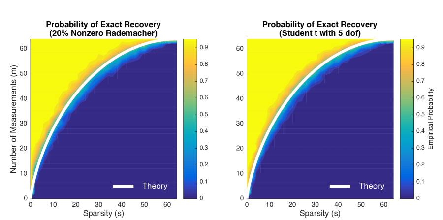
Figure 5.1. Universality of the $\ell_{1}$ Recovery Phase Transition. These plots depict the empirical probability that the $\ell_{1}$ minimization problem (5.1) recovers a vector $\bm{x}_{\star}\in\mathbb{R}^{64}$ with $s$ nonzero entries from a vector of random measurements $\bm{y}=\bm{\Phi}\bm{x}_{\star}\in\mathbb{R}^{m}$. The heatmap indicates the empirical probability, computed over 100 trials. The white curve is the phase transition $n\psi_{\ell_{1}}(s/n)$ promised by Proposition 5.1. Left: The random measurement matrix $\bm{\Phi}$ is a sparse Rademacher matrix with an average of 20% nonzero entries. Right: The random measurement matrix $\bm{\Phi}$ has independent Student $t_{5}$ entries. See Section 1.9 for more details.

Proposition 5.1 (Universality of $\ell_{1}$ Phase Transition).

Assume that

• The ambient dimension $n$ and the number $m$ of measurements satisfy $m\leq n$.

• The vector $\bm{x}_{\star}\in\mathbb{R}^{n}$ has exactly $s$ nonzero entries.

• The random measurement matrix $\bm{\Phi}:\mathbb{R}^{n}\to\mathbb{R}^{m}$ follows Model 2.4 with parameters $p$ and $\nu$.

• We observe the vector $\bm{y}=\bm{\Phi}\bm{x}_{\star}$.

Then, as the ambient dimension $n\to\infty$,

$$m/n <\psi_{\ell_{1}}(s/n)-o(1)\quad\text{implies}\quad\text{\eqref{eqn:l1-min} fails with probability $1-o(1)$;}$$

$$m/n >\psi_{\ell_{1}}(s/n)+o(1)\quad\text{implies}\quad\text{\eqref{eqn:l1-min} succeeds with probability $1-o(1)$.}$$

The little-o suppresses constants that depend only on $p$ and $\nu$.

Proposition 5.1 follows directly from our universality result, Theorem I, and the established calculation (5.3) of the phase transition in the standard normal setting.

Proof.

The approach is quite standard. Let $\Omega$ be the set of unit-norm descent directions of the $\ell_{1}$ norm at the point $\bm{x}_{\star}$. That is,

$$\Omega:=\big{\{}\bm{u}\in\mathsf{S}^{n-1}:\left\|{\bm{x}_{\star}+\lambda\bm{u}}\right\|_{1}\leq\left\|{\bm{x}_{\star}}\right\|_{1}\text{ for some $\lambda>0$}\big{\}}.$$

The primal optimality condition for (5.1) demonstrates that the reconstruction succeeds if and only if $\Omega\cap\operatorname{null}(\bm{\Phi})=\emptyset$. Since the $\ell_{1}$ norm is a closed convex function, the set $\bm{\theta}^{-1}(\Omega)\cup\{\bm{0}\}$ of all descent directions forms a closed, convex cone. Therefore, the set $\Omega$ is closed and spherically convex. It follows from Theorem I that the behavior of (5.1) undergoes a phase transition at the statistical dimension $\delta(\Omega)$ for any random linear map drawn from Model 2.4.

The result [ALMT14, Prop. 4.5] contains the first complete and accurate computation of the statistical dimension of a descent cone of the $\ell_{1}$ norm:

$$n\psi_{\ell_{1}}(s/n)-O(\sqrt{n})\leq\delta(\Omega)\leq n\psi_{\ell_{1}}(s/n).$$ (5.4)

See also [FM14, Prop. 1]. This fact completes the proof. ∎

Note that Proposition 5.1 requires the sparsity level $s$ to be proportional to the ambient dimension $n$ before it provides any information. By refining our argument, we can address the case when $s$ is proportional to $n^{1-\varepsilon}$ for a small number $\varepsilon$ that depends on the regularity of the random linear map. The empirical work [DT09a] of Donoho & Tanner is unable to provide statistical evidence for the universality hypothesis in the regime where $s$ is very small. It remains an open problem to understand how rapidly $s/n$ can vanish before the universality phenomenon fails.

The paper [DT09a] also contains numerical evidence that the $\ell_{1}$ phase transition persists for random measurement systems that have more structure than Model 2.4. It remains an intriguing open question to understand these experiments.

Remark 5.2 (Prior Work).

In early 2005, Donoho [Don06c] and Donoho & Tanner [DT06] observed that there is a phase transition in the number of standard normal measurements needed to reconstruct a sparse signal via $\ell_{1}$ minimization. Using methods from integral geometry, they were able to perform a heuristic computation of the location of the phase transition function (5.2). In subsequent work [DT09b], they proved that the transition (5.3) is valid in some parameter regimes. They later reported extensive empirical evidence [DT09a] that the distribution of the random measurement map has little effect on the location of the phase transition.

In early 2005, Rudelson & Vershynin [RV08] proposed a different approach to studying $\ell_{1}$ minimization by adapting results of Gordon [Gor88] that depend on Gaussian process theory. Stojnic [Sto09] refined this argument to obtain an empirically sharp success condition for standard normal linear maps, but his work did not establish a matching failure condition. Stojnic’s calculations were clarified and extended to other signal recovery problems in the papers [OH10, CRPW12, ALMT14, FM14].

Bayati et al. [BLM15] is the first paper to rigorously demonstrate that the phase transition (5.3) is valid for standard normal measurements. The argument is based on a state evolution framework for an iterative algorithm inspired by statistical physics. This work also gives the striking conclusion that the $\ell_{1}$ phase transition is universal over a class of random measurement maps. This result requires the measurement matrix to have independent, standardized, subgaussian entries that are absolutely continuous with respect to the Gaussian distribution. As a consequence, the paper [BLM15] excludes discrete and heavy-tailed models. Furthermore, it only applies to $\ell_{1}$ minimization. In contrast, Proposition 5.1 and its proof have a much wider compass.

The paper [ALMT14] of Amelunxen et al. contains the first complete integral-geometric proof of (5.3) for standard normal measurements. This work is significant because it established for the first time that phase transitions are ubiquitous in signal reconstruction problems. It also forged the first links between the approach to phase transitions based on integral geometry and those based on Gaussian process theory. The papers [MT14a, GNP14] build on these ideas to obtain precise estimates of the success probability in (5.3).

Subsequently, Stojnic [Sto13] refined the Gaussian process methods to obtain more detailed information about the behavior of the errors in noisy variants of the $\ell_{1}$ minimization problem. His work has been extended in a series [OTH13, TOH15, TAH15] of papers by Abbasi, Oymak, Thrampoulidis, Hassibi, and their collaborators. Because of this research, we now have a very detailed understanding of the behavior of convex signal recovery methods with Gaussian measurements.

To our knowledge, the current paper is the first work that extends the type of general analysis in [ALMT14, OTH13, TAH15] beyond the confines of the standard normal model.

5.2. Other Signal Recovery Problems

The compressed sensing problem is the most prominent example from a large class of related questions. Our universality results have implications for this entire class of problems. We include a brief explanation.

Let $f:\mathbb{R}^{n}\to\mathbb{R}$ be a proper convex function whose value increases with the “complexity” of its argument. The $\ell_{1}$ norm is an example of a complexity measure that is appropriate for sparse signals [CDS98]. Similarly, the Schatten 1-norm is a good complexity measure for low-rank matrices [Faz02].

Let $\bm{x}_{\star}\in\mathbb{R}^{n}$ be a vector with “low complexity.” Draw a random linear map $\bm{\Phi}:\mathbb{R}^{n}\to\mathbb{R}^{m}$, and suppose we have access to $\bm{x}_{\star}$ only through the measurements $\bm{y}=\bm{\Phi}\bm{x}_{\star}$. We can attempt to reconstruct $\bm{x}_{\star}$ by solving the convex optimization problem

$$\underset{\bm{x}\in\mathbb{R}^{n}}{\quad\text{minimize}\quad}f(\bm{x})\quad\text{subject to}\quad\bm{\Phi}\bm{x}=\bm{y}.$$

In other words, we find the vector with minimum complexity that is consistent with the observed data. We say that (5.2) succeeds when it has a unique optimal point that coincides with $\bm{x}_{\star}$; otherwise, it fails.

The paper [ALMT14] proves that there is a phase transition in the behavior of (5.2) when $\bm{\Phi}$ is standard normal. Our universality law, Theorem I, allows us to extend this result to include every random linear map from Model 2.4. Define the set $\Omega$ of unit-norm descent directions of $f$ at the point $\bm{x}_{\star}$:

$$\Omega:=\big{\{}\bm{u}\in\mathsf{S}^{n-1}:f(\bm{x}_{\star}+\lambda\bm{u})\leq f(\bm{x}_{\star})\text{ for some $\lambda>0$}\big{\}}.$$

Then, as the ambient dimension $n\to\infty$,

$$m <\delta(\Omega)-o(n)\quad\text{implies}\quad\text{\eqref{eqn:f-min} fails with probability $1-o(1)$};$$

$$m >\delta(\Omega)+o(n)\quad\text{implies}\quad\text{\eqref{eqn:f-min} succeeds with probability $1-o(1)$}.$$

In other words, there is a phase transition in the behavior of (5.2) when the number $m$ of measurements equals the statistical dimension $\delta(\Omega)$ of the set of descent directions of $f$ at the point $\bm{x}_{\star}$. See the papers [CRPW12, ALMT14, FM14] for some general methods for computing the statistical dimension of a descent cone.

5.3. Complements

We conclude this section with a few additional remarks about the scope of our results on signal recovery. First, we discuss some geometric applications. Second, we mention some other signal processing problems that can be studied using the same methods.

5.3.1. Geometric Implications

Proposition 5.1 can be understood as a statement about the facial structure of a random projection of the $\ell_{1}$ ball. Equivalently, it provides information about the facial structure of the convex hull of random points.

Suppose that $\mathsf{B}_{1}^{n}$ is the $n$-dimensional $\ell_{1}$ ball, and fix an $(s-1)$-dimensional face $F$ of $\mathsf{B}_{1}^{n}$. Let $\bm{\Phi}:\mathbb{R}^{n}\to\mathbb{R}^{m}$ be a random linear map from Model 2.4. We say that $\bm{\Phi}$ preserves the face $F$ when $\bm{\Phi}(F)$ is an $(s-1)$-dimensional face of the projection $\bm{\Phi}(\mathsf{B}_{1}^{n})$. We can reinterpret Proposition 5.1 as saying that

$$m/n <\psi_{\ell_{1}}(s/n)-o(1)\quad\text{implies}\quad\text{$\bm{\Phi}$ is unlikely to preserve $F$;}$$

$$m/n >\psi_{\ell_{1}}(s/n)+o(1)\quad\text{implies}\quad\text{$\bm{\Phi}$ is likely to preserve $F$.}$$

The connection between $\ell_{1}$ minimization and the facial structure of the $\ell_{1}$ ball was identified in [Don06b]; see also [ALMT14, Sec. 10.1.1].

Here is another way of framing the same result. Fix an index set $J\subset\{1,\dots,n\}$ with cardinality $\#J=s$ and a vector $\bm{\eta}\in\mathbb{R}^{n}$ with $\pm 1$ entries. Let $\bm{\varphi}_{1},\dots,\bm{\varphi}_{n}\in\mathbb{R}^{m}$ be independent random vectors, drawn from Model 2.4, and consider the absolute convex hull $E:=\operatorname{conv}\{\pm\bm{\varphi}_{1},\dots,\pm\bm{\varphi}_{n}\}$. The question is whether the set $F:=\operatorname{conv}\{\eta_{j}\bm{\varphi}_{j}:j\in J\}$ is an $(s-1)$-dimensional face of $E$. We have the statements

$$s/n <\psi_{\ell_{1}}^{-1}(m/n)-o(1)\quad\text{implies}\quad\text{$F$ is likely to be an $(s-1)$-dimensional face of $E$;}$$

$$s/n >\psi_{\ell_{1}}^{-1}(m/n)+o(1)\quad\text{implies}\quad\text{$F$ is unlikely to be an $(s-1)$-dimensional face of $E$.}$$

See the paper [DT09b] for more discussion of the connection between the facial structure of polytopes and signal recovery. Some universality results of this type also appear in Bayati et al. [BLM15].

5.3.2. Other Signal Processing Applications

We often want to perform signal processing tasks on data after reducing its dimension. In this section, we have focused on the problem of reconstructing a sparse signal from random measurements. Here are some related problems:

• Detection. Does an observed signal consist of a template corrupted with noise? Or is it just noise?

• Classification. Does an observed signal belong to class A or to class B?

The literature contains many papers that propose methods for solving these problems after dimension reduction; for example, see [DDW⁺07]. The existing analysis is either qualitative or it assumes that the dimension reduction map is Gaussian. Our universality laws can be used to study the precise behavior of compressed detection and classification with more general types of random linear maps. For brevity, we omit the details.

6. Decoding with Structured Errors

One of the goals of coding theory is to design codes and decoding algorithms that can correct gross errors in transmission. In particular, it is common that some proportion of the received symbols are corrupted. In this section, we show that a large family of random codes can be decoded in the presence of structured errors. The number of errors that we can correct is universal over this family. This result is valuable because it applies to random codebooks that are closer to realistic coding schemes.

The result on random decoding can also be interpreted as a statement about the behavior of the least-absolute-deviation (LAD) method for regression. We also discuss how our universality results apply to a class of demixing problems.

6.1. Decoding with Sparse Errors

We work with a random linear code over the real field. Consider a fixed message $\bm{x}_{\star}\in\mathbb{R}^{m}$. Let $\bm{\Phi}\in\mathbb{R}^{n\times m}$ be a random matrix, which is called a codebook in this context. Instead of transmitting the original message $\bm{x}_{\star}$, we transmit the coded message $\bm{\Phi}\bm{x}_{\star}$. Suppose that we receive a version $\bm{y}$ of the message where some number $s$ of the entries are corrupted. That is, $\bm{y}=\bm{\Phi}\bm{x}_{\star}+\bm{z}_{\star}$ where the error vector $\bm{z}_{\star}$ has at most $s$ nonzero entries. For simplicity, we assume that $\bm{z}_{\star}$ does not depend on the codebook $\bm{\Phi}$.

In this setting, one can attempt to decode the message using an $\ell_{1}$ minimization method [DH01, CRTV05, DT06, MT14b]. We solve the optimization problem

$$\underset{\bm{x}\in\mathbb{R}^{m},\bm{z}\in\mathbb{R}^{n}}{\quad\text{minimize}\quad}\left\|{\bm{z}}\right\|_{\ell_{1}}\quad\text{subject to}\quad\bm{y}=\bm{\Phi}\bm{x}+\bm{z}.$$ (6.1)

In other words, we search for a message $\bm{x}$ and a sparse corruption $\bm{z}$ that match the received data. We say that the optimization (6.1) succeeds if it has a unique optimal point $(\widehat{\bm{x}},\widehat{\bm{z}})$ that coincides with $(\bm{x}_{\star},\bm{z}_{\star})$; otherwise it fails.

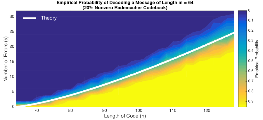
Figure 6.1. Universality of the $\ell_{1}$ Decoding Phase Transition. This plot shows the empirical probability that the $\ell_{1}$ method (6.1) decodes the message $\bm{x}_{\star}\in\mathbb{R}^{64}$ from the received message $\bm{y}=\bm{\Phi}\bm{x}_{\star}+\bm{z}_{\star}\in\mathbb{R}^{n}$ where the corruption $\bm{z}_{\star}\in\mathbb{R}^{n}$ has exactly $s$ nonzero entries. The codebook $\bm{\Phi}\in\mathbb{R}^{n\times 64}$ is a sparse Rademacher matrix with an average of 20% nonzero entries. The heatmap gives the empirical probability of correct decoding, computed over 100 trials. The white curve is the exact phase transition $n\psi_{\ell_{1}}^{-1}(1-64/n)$ promised by Proposition 6.1. See Section 1.9 for more details.

The question is when the optimization problem (6.1) is effective at decoding the received transmission. That is, how many errors $s$ can we correct as a function of the message length $m$ and the code length $n$? The following result gives a solution to this problem for any codebook drawn from Model 2.4.

Proposition 6.1 (Universality of Sparse Error Correction).

Assume that

• The message length $m$ and the code length $n$ satisfy $m\leq n$.

• The message $\bm{x}_{\star}\in\mathbb{R}^{m}$ is arbitrary.

• The error vector $\bm{z}_{\star}\in\mathbb{R}^{n}$ has exactly $s$ nonzero entries, where $s\leq(1-\xi)n$ for some $\xi>0$.

• The random codebook $\bm{\Phi}\in\mathbb{R}^{n\times m}$ follows Model 2.4 with parameters $p$ and $\nu$.

• We observe the vector $\bm{y}=\bm{\Phi}\bm{x}_{\star}+\bm{z}_{\star}$.

Then, as the message length $m\to\infty$,

$$s/n <\psi_{\ell_{1}}^{-1}(1-m/n-o(1))\quad\text{implies}\quad\quad\text{\eqref{eqn:l1-decode} succeeds with probability $1-o(1)$;}$$

$$s/n >\psi_{\ell_{1}}^{-1}(1-m/n+o(1))\quad\text{implies}\quad\quad\text{\eqref{eqn:l1-decode} fails with probability $1-o(1)$.}$$

The function $\psi_{\ell_{1}}$ is defined in (5.2). The little-o suppresses constants that depend only on $\xi$ and $p$ and $\nu$.

This result is significant because it allows us to understand the behavior of this method for a sparse, discrete codebook. This type of code is somewhat closer to a practical coding mechanism than the ultra-random codebooks that have been studied in the past; see Remark 6.3. Figure 6.1 contains an illustration of how the theory compares with the actual performance of this coding scheme.

Proof.

To analyze the decoding problem (6.1), we change variables: $\bm{u}:=\bm{x}-\bm{x}_{\star}$ and $\bm{v}:=\bm{z}-\bm{z}_{\star}$. We obtain the equivalent optimization problem

$$\underset{\bm{u}\in\mathbb{R}^{m},\bm{v}\in\mathbb{R}^{n}}{\quad\text{minimize}\quad}\left\|{\bm{z}_{\star}+\bm{v}}\right\|_{\ell_{1}}\quad\text{subject to}\quad\bm{\Phi}\bm{u}=\bm{v}.$$ (6.2)

The decoding procedure (6.1) succeeds if and only if the unique optimal point $(\widehat{\bm{u}},\widehat{\bm{v}})$ of the problem (6.2) is the pair $(\bm{0},\bm{0})$.

Introduce the set $\Omega$ of unit-norm descent directions of the $\ell_{1}$ norm at $\bm{z}_{\star}$:

$$\Omega:=\big{\{}\bm{v}\in\mathsf{S}^{n-1}:\left\|{\bm{z}_{\star}+\lambda\bm{v}}\right\|_{\ell_{1}}\leq\left\|{\bm{z}_{\star}}\right\|_{\ell_{1}}\text{ for some $\lambda>0$}\big{\}}.$$

The primal optimality condition for (6.2) shows that decoding succeeds if and only if $\Omega\cap\operatorname{range}(\bm{\Phi})=\emptyset$.

Let us compute the statistical dimension of $\Omega^{\circ}$:

$$\delta(\Omega^{\circ})=n-\delta(\Omega)=n-(n\psi_{\ell_{1}}(s/n)+o(n))=n(1-\psi_{\ell_{1}}(s/n)+o(1)).$$ (6.3)

The first relation is the polar identity (3.5) for the statistical dimension, and the value of the statistical dimension appears in (5.4). Since $s\leq(1-\xi)n$, the properties of the function $\psi_{\ell_{1}}$ ensure that $\delta(\Omega^{\circ})\geq\varrho n$ for some $\varrho>0$.

First, we demonstrate that decoding fails when the number $s$ of errors is too large. To do so, we must show that $\Omega\cap\operatorname{range}(\bm{\Phi})\neq\emptyset$. By polarity [Kle55, Thm. (2.7)], it suffices to check that

$$\Omega^{\circ}\cap\operatorname{null}(\bm{\Phi}^{*})=\emptyset.$$

With probability at least $1-o(1)$, this relation follows from Theorem I(a), provided that

$$m>\delta(\Omega^{\circ})+o(n)=n(1-\psi_{\ell_{1}}(s/n))+o(n).$$

Finally, revert the inequality so that it is expressed in terms of $s$.

Last, we must check that decoding succeeds when the number $s$ of errors is sufficiently small. To do so, we must verify that $\Omega\cap\operatorname{range}(\bm{\Phi})=\emptyset$ with high probability. This relation follows from ideas closely related to the proof of Theorem I, but it is not a direct consequence. See Section 17.3 for the details. ∎

Remark 6.2 (Least-Absolute-Deviation Regression).

Proposition 6.1 can also be interpreted as a statement about the performance of the least-absolute deviation method for fitting models with outliers. Suppose that we observe the data $\bm{y}=\bm{X}\bm{\beta}_{\star}+\bm{z}$. Each of the $n$ rows of $\bm{X}$ is interpreted as a vector of $m$ measured variables for an independent subject in an experiment. The vector $\bm{\beta}_{\star}$ lists the coefficients in the true linear model, and the sparse vector $\bm{z}$ contains a small number $s$ of arbitrary statistical errors. The least-absolute deviation method fits a model by solving

$$\underset{\bm{\beta}\in\mathbb{R}^{m}}{\quad\text{minimize}\quad}\left\|{\smash{\bm{X}\bm{\beta}-\bm{y}}}\right\|_{\ell_{1}}.$$

Proposition 6.1 shows that the procedure identifies the true model $\bm{\beta}_{\star}$ exactly, provided that the number $s$ of contaminated data points satisfies $s/n<\psi_{\ell_{1}}^{-1}(1-m/n)-o(1)$.

Remark 6.3 (Prior Work).

The idea of using $\ell_{1}$ minimization for decoding in the presence of sparse errors dates at least as far back as the paper [DH01]. This scheme received further attention in the work [CRTV05]. Later, Donoho & Tanner [DT06] applied phase transition calculations to assess the precise performance of this coding scheme for a standard normal codebook; the least-absolute-deviation interpretation of this result appears in [DT09a, Sec. 1.3]. The paper [MT14b] revisits the coding problem and develops a sharp analysis in the case where the codebook is a random orthogonal matrix. The current paper contains the first precise result that extends to codebooks with more general distributions.

6.2. Other Demixing Problems

The decoding problem (6.1) is an example of a convex demixing problem [MT14b, ALMT14]. Our universality results can be used to study other questions of this species.

Let $f_{0}:\mathbb{R}^{n}\to\mathbb{R}$ and $f_{1}:\mathbb{R}^{n}\to\mathbb{R}$ be proper convex functions that measure the complexity of a signal. Suppose that $\bm{x}_{\star}^{0}\in\mathbb{R}^{n}$ and $\bm{x}_{\star}^{1}\in\mathbb{R}^{n}$ are signals with “low complexity.” Draw random matrices $\bm{\Phi}_{0}:\mathbb{R}^{n}\to\mathbb{R}^{m}$ and $\bm{\Phi}_{1}:\mathbb{R}^{n}\to\mathbb{R}^{m}$ from Model 2.4. Suppose that we observe the vector $\bm{y}=\bm{\Phi}_{0}\bm{x}_{\star}^{1}+\bm{\Phi}_{1}\bm{x}_{\star}^{1}$. We interpret the random matrices as known transformations of the unknown signals. For example, the matrices $\bm{\Phi}_{i}$ might denote dictionaries in which the two components of $\bm{y}$ are sparse.

We can attempt to reconstruct the original signal pair by solving

$$\underset{\bm{z}^{0}\in\mathbb{R}^{n},\bm{z}^{1}\in\mathbb{R}^{n}}{\quad\text{minimize}\quad}\max\big{\{}f_{0}(\bm{z}^{0}),f_{1}(\bm{z}^{1})\big{\}}\quad\text{subject to}\quad\bm{\Phi}_{0}\bm{z}^{0}+\bm{\Phi}_{1}\bm{z}^{1}=\bm{y}.$$ (6.4)

In other words, we witness a superposition of two structured signals, and we attempt to find the lowest complexity pair $(\bm{z}^{0},\bm{z}^{1})$ that reproduces the observed data. The demixing problem succeeds if it has a unique optimal point that equals $(\bm{x}_{\star}^{0},\bm{x}_{\star}^{1})$.

To analyze this problem, we introduce two descent sets:

$$\Omega_{i}:=\big{\{}\bm{u}\in\mathsf{S}^{n-1}:f_{i}(\bm{x}_{\star}^{i}+\lambda\bm{u})\leq f_{i}(\bm{x}_{\star}^{i})\text{ for some $\lambda>0$}\big{\}}\quad\text{for $i=1,2$.}$$

Up to scaling, the descent directions of $\max\{f_{0}(\cdot),f_{1}(\cdot\cdot)\}$ at the pair $(\bm{x}_{\star}^{0},\bm{x}_{\star}^{1})$ coincide with the direct product $\Omega_{0}\times\Omega_{1}$. The statistical dimension of a direct product of two spherical sets satisfies $\delta(\Omega_{0}\times\Omega_{1})=\delta(\Omega_{0})+\delta(\Omega_{1})$. Therefore, Theorem I demonstrates that

$$m <\delta(\Omega_{0})+\delta(\Omega_{1})-o(n)\quad\text{implies}\quad\text{\eqref{eqn:demix} fails with probability $1-o(1)$;}$$

$$m >\delta(\Omega_{0})+\delta(\Omega_{1})+o(n)\quad\text{implies}\quad\text{\eqref{eqn:demix} succeeds with probability $1-o(1)$.}$$

In other words, the amount of information needed to extract a pair of signals from the superposition equals the total complexity of the two signals. This result holds true for a wide class of distributions on $\bm{\Phi}_{0}$ and $\bm{\Phi}_{1}$.

7. Randomized Numerical Linear Algebra

Numerical linear algebra (NLA) is the study of computational methods for problems in linear algebra, including the solution of linear systems, spectral calculations, and matrix approximations. Over the last 15 years, researchers have developed many new algorithms for NLA that exploit randomness to perform these computations more efficiently. See the surveys [Mah11, HMT11, Woo14] for an overview of this field.

In this section, we apply our universality techniques to obtain new results on dimension reduction in randomized NLA. This discussion shows that a broad class of dimension reduction methods share the same quantitative behavior. Therefore, within some limits, we can choose the random linear map that is most computationally appealing when we design numerical algorithms based on dimension reduction.

As an added bonus, the arguments here lead to a new proof of the Bai–Yin limit for the minimum singular value of a random matrix drawn from Model 2.4.

7.1. Subspace Embeddings

In randomized NLA, one of the key primitives is a subspace embedding. A subspace embedding is nothing more than a randomized linear map that does not annihilate any point in a fixed subspace.

Definition 7.1 (Subspace Embedding).

Fix a natural number $k$, and let $L$ be an arbitrary $k$-dimensional subspace. We say that a randomized linear map $\bm{\Pi}:\mathbb{R}^{D}\to\mathbb{R}^{d}$ is an oblivious subspace embedding of order $k$ if

$$\bm{0}\notin\bm{\Pi}\big{(}L\cap\mathsf{S}^{D-1}\big{)}\quad\text{with high probability.}$$

The term “oblivious” indicates that the linear map $\bm{\Pi}$ is chosen without knowledge of the subspace $L$.

In the definition of a subspace embedding, some authors include quantitative bounds on the stability of the embedding. These estimates are useful for analyzing certain algorithms, but we have left them out because they are not essential.

A standard normal matrix provides an important theoretical and practical example of a subspace embedding.

Example 7.2 (Gaussian Subspace Embedding).

For any natural number $k$, a standard normal matrix $\bm{\Gamma}\in\mathbb{R}^{d\times D}$ is a subspace embedding with probability one when the embedding dimension $d\geq k$. In practice, it is preferable to select the embedding dimension $d\geq k+10$ to ensure that the restricted singular value $\sigma_{\min}(\bm{\Gamma};L\cap\mathsf{S}^{D-1})$ is sufficiently positive, which makes the embedding more stable. See [HMT11] for more details.

A Gaussian subspace embedding has superb dimension reduction properties. On the other hand, standard normal matrices are expensive to generate, to store, and to perform arithmetic with. Therefore, in most randomized NLA algorithms, it is better to use subspace embeddings that are discrete or sparse.

Our universality results demonstrate that, in a certain range of parameters, every matrix that follows Model 2.4 enjoys the same subspace embedding properties as a Gaussian matrix.

Proposition 7.3 (Universality for Subspace Embedding).

Suppose that

• The ambient dimension $D$ is sufficiently large.

• The embedding dimension satisfies $d\leq D^{6/5}$.

• The random linear map $\bm{\Pi}:\mathbb{R}^{D}\to\mathbb{R}^{d}$ follows Model 2.4 with parameters $p$ and $\nu$.

Then, for each $k$-dimensional subspace $L$ of $\mathbb{R}^{D}$,

$$\sigma_{\min}(\bm{\Pi};L\cap\mathsf{S}^{D-1})\geq\sqrt{d}-\sqrt{k}-o(\sqrt{D})\quad\text{with probability $1-o(1)$.}$$

In particular, $\bm{\Pi}$ is a subspace embedding of order $k$ whenever $d\geq k+o(D)$. In these expressions, the little-o suppresses constants that depend only on $p$ and $\nu$.

Proof.

Proposition 7.3 is a consequence of Theorem II(a) and (4.3) because

$$\mathscr{E}_{d}(L\cap\mathsf{S}^{D-1})\geq\sqrt{d}-\sqrt{\delta(L\cap\mathsf{S}^{D-1})}=\sqrt{d}-\sqrt{\delta(L)}=\sqrt{d}-\sqrt{k}.$$

The last identity holds because the $k$-dimensional subspace $L$ has statistical dimension $k$. We introduce the error term $o\big{(}\sqrt{D}\big{)}$ to make sure that the stated result is only valid when the hypotheses of Theorem II are in force. ∎

Note that Proposition 7.3 applies to a sparse Rademacher linear map with a fixed, but arbitrarily small, proportion of nonzero entries. This particular example has received extensive attention in recent years [CW13, NN13, KN14, BDN15], although these works typically focus on the regime where the subspace dimension $k$ is small and the sparsity level of the random linear map is a vanishing proportion of the embedding dimension $d$.

Remark 7.4 (Prior Work).

For the simple problem considered in Proposition 7.3, much sharper results are available in the random matrix literature. See the paper [KY14] for a recent analysis, as well as additional references.

Remark 7.5 (The Bai–Yin Limit for the Minimum Singular Value).

One of the most important problems in random matrix theory is to obtain bounds for the extreme singular values of a random matrix. The Bai–Yin law [BY93] gives a near-optimal result in case the entries of the random matrix are independent and standardized. We can reproduce a slightly weaker version of the Bai–Yin law for the minimum singular value by modifying the proof of Proposition 7.3.

Fix an aspect ratio $\varrho\in(0,1)$. For each natural number $d$, define $k:=k(d):=\lfloor\varrho d\rfloor$. Draw a $d\times k$ random matrix $\bm{\Phi}^{(d)}$ from Model 2.4 with fixed parameters $p$ and $\nu$. For each $\varepsilon>0$, we can apply Theorem II(a) with $E=\mathsf{S}^{k-1}$ to see that

$$\mathbb{P}\left\{{d^{-1/2}\sigma_{\min}\big{(}\bm{\Phi}^{(d)}\big{)}\geq 1-\sqrt{\varrho}-\varepsilon}\right\}\to 1\quad\text{as $d\to\infty$}.$$

Here, $\sigma_{\min}$ denotes the $k$th largest singular value of $\bm{\Phi}^{(d)}$.

Under these assumptions, it is known [Yin86] that the empirical distribution of the singular values of $\bm{\Phi}^{(d)}$ converges in probability to the Marčenko–Pastur density, whose support is the interval $1\pm\sqrt{\varrho}$. It follows that

$$\mathbb{P}\left\{{d^{-1/2}\sigma_{\min}\big{(}\bm{\Phi}^{(d)}\big{)}\leq 1-\sqrt{\varrho}+\varepsilon}\right\}\to 1\quad\text{as $d\to\infty$}.$$

Therefore, we may conclude that

$$d^{-1/2}\sigma_{\min}\big{(}\bm{\Phi}^{(d)}\big{)}\to 1-\sqrt{\varrho}\quad\text{in probability.}$$

In comparison, the Bai–Yin law [BY93, Thm. 2] gives the same conclusion almost surely when the entries of $\bm{\Phi}^{(d)}$ have four finite moments. See the recent paper [Tik15] for an optimal result.

7.2. Sketching and Least Squares

In randomized NLA, one of the core applications of dimension reduction is to solve over-determined least-squares problems, perhaps with additional constraints. This idea is attributed to Sarlós [Sar06], and it has been studied intensively over the last decade; see the surveys [Mah11, Woo14] for more information. In this section, we develop sharp bounds for the simplest version of this approach.

Suppose that $\bm{A}$ is a fixed $D\times n$ matrix with full column rank. Let $\bm{y}\in\mathbb{R}^{D}$ be a vector, and consider the over-determined least-squares problem

$$\underset{\bm{x}\in\mathbb{R}^{n}}{\quad\text{minimize}\quad}\left\|{\smash{\bm{A}\bm{x}-\bm{y}}}\right\|^{2}.$$ (7.1)

This problem can be expensive to solve when $D\gg n$. One remedy is to apply dimension reduction. Draw a random linear map $\bm{\Pi}:\mathbb{R}^{D}\to\mathbb{R}^{d}$ from Model 2.4, and consider the compressed problem

$$\underset{\bm{x}\in\mathbb{R}^{n}}{\quad\text{minimize}\quad}\left\|{\smash{\bm{\Pi}(\bm{A}\bm{x}-\bm{y})}}\right\|^{2}.$$ (7.2)

The question is how the quality of the solution of (7.2) depends on the embedding dimension $d$. The following result provides an optimal estimate.

Proposition 7.6 (Randomized Least Squares: Error Bound).

Instate the prevailing notation. Fix parameters $\lambda\in(0,1)$ and $\varrho\in(0,1)$ and $\iota\in(0,1)$. Assume that

• The number $D$ of constraints is sufficiently large as a function of the parameters.

• The embedding dimension $d$ is comparable with the number $D$ of constraints: $\lambda D\leq d\leq D$.

• The embedding dimension $d$ is somewhat larger than the number $n$ of variables: $d\geq(1+\varrho)n$.

With high probability, the solution $\widehat{\bm{x}}$ to the reduced least-squares problem (7.2) satisfies

$$\frac{\left\|{\bm{A}(\widehat{\bm{x}}-\bm{x}_{\star})}\right\|^{2}}{\left\|{\smash{\bm{A}\bm{x}_{\star}-\bm{y}}}\right\|^{2}}\leq\frac{n+\iota d}{d-n},$$ (7.3)

where $\bm{x}_{\star}$ is the solution to the original least-squares problem (7.1). In particular,

$$\frac{\left\|{\smash{\bm{A}\widehat{\bm{x}}-\bm{y}}}\right\|^{2}}{\left\|{\smash{\bm{A}\bm{x}_{\star}-\bm{y}}}\right\|^{2}}\leq(1+\iota)\frac{d}{d-n}$$

In other words, the excess error $\left\|{\bm{A}(\widehat{\bm{x}}-\bm{x}_{\star})}\right\|$ incurred in solving the compressed least-squares problem (7.2) is negligible as compared with the optimal value of the least-squares problem (7.1) if we choose the embedding dimension $d$ sufficiently large. Proposition 7.6 improves substantially on the most recent work [PW15, Cor. 2(a)], both in terms of the error bound and in terms of the assumptions on the randomized linear map.

Let us remark that there is nothing special about ordinary least squares. We can also solve least-squares problems with a convex constraint set by dimension reduction. For this class of problems, we can also obtain optimal bounds by adapting the argument below. For example, see the results in Section 8.

Proof.

Let $\bm{x}_{\star}\in\mathbb{R}^{n}$ be the solution to the original least-squares problem (7.1). Define the optimal residual $\bm{z}_{\star}:=\bm{y}-\bm{A}\bm{x}_{\star}\in\mathbb{R}^{D}$, and recall that $\bm{z}_{\star}$ is orthogonal to $\operatorname{range}(\bm{A})$. Moreover,

$$\min_{\bm{x}\in\mathbb{R}^{n}}\left\|{\smash{\bm{A}\bm{x}-\bm{y}}}\right\|^{2}=\left\|{\smash{\bm{A}\bm{x}_{\star}-\bm{y}}}\right\|^{2}=\left\|{\bm{z}_{\star}}\right\|^{2}.$$

Without loss of generality, we may scale the problem so that $\left\|{\bm{z}_{\star}}\right\|^{2}=1$.

Next, change variables. Define $\bm{w}:=\bm{A}(\bm{x}-\bm{x}_{\star})$, and note that $\bm{w}$ is orthogonal to $\bm{z}_{\star}$. We can write the reduced least-squares problem (7.2) as

$$\underset{\bm{w}\in\operatorname{range}(\bm{A})}{\quad\text{minimize}\quad}\left\|{\bm{\Pi}(\bm{w}-\bm{z}_{\star})}\right\|.$$ (7.4)

When dimension reduction is effective, we expect the solution $\widehat{\bm{w}}$ to (7.4) to be close to zero.

Since $d\geq(1+\varrho)n$, we can use the fact (Proposition 7.3) that $\bm{\Pi}$ is a subspace embedding to obtain an a priori bound $\left\|{\widehat{\bm{w}}}\right\|\leq R_{\infty}$ that holds with high probability. The number $R_{\infty}$ is a constant that depends on nothing but $\varepsilon$. We only need this observation to ensure that we are optimizing over a compact set with constant radius, so we omit the details.

Next, we invoke Theorem II(b) to bound the optimal value of the reduced least-squares problem (7.4). Define the compact, convex set

$$E:=\{\bm{w}\in\operatorname{range}(\bm{A}):\left\|{\bm{w}}\right\|\leq R_{\infty}\}.$$

Let $\varepsilon>0$ be a parameter that will depend on the parameter $\iota$. With high probability,

$$\min_{\bm{w}\in\operatorname{range}(\bm{A})}\left\|{\bm{\Pi}(\bm{w}-\bm{z}_{\star})}\right\|=\min_{\bm{w}\in E}\left\|{\bm{\Pi}(\bm{w}-\bm{z}_{\star})}\right\|\leq(1+\varepsilon)\,\mathscr{E}_{d}(E-\bm{z}_{\star}).$$

By direct calculation, we can bound the excess width above. Let $\bm{P}$ be the orthogonal projector onto the range of $\bm{A}$, and observe that

$$\mathscr{E}_{d}(E-\bm{z}_{\star}) =\operatorname{\mathbb{E}}\inf_{\bm{w}\in E}\big{(}\sqrt{d}\left\|{\bm{w}-\bm{z}_{\star}}\right\|+\bm{g}\cdot(\bm{w}-\bm{z}_{\star})\big{)}$$

$$=\operatorname{\mathbb{E}}\inf_{\bm{w}\in E}\big{(}\sqrt{d}(\left\|{\bm{w}}\right\|^{2}+1)^{1/2}+\bm{g}\cdot\bm{w}\big{)}$$

$$=\operatorname{\mathbb{E}}\inf_{\bm{w}\in E}\big{(}\sqrt{d}(\left\|{\bm{w}}\right\|^{2}+1)^{1/2}-\left\|{\smash{\bm{P}\bm{g}}}\right\|\left\|{\bm{w}}\right\|\big{)}$$

$$\leq\inf_{0\leq\alpha\leq R_{\infty}}\big{(}\sqrt{d}(\alpha^{2}+1)^{1/2}-\sqrt{n}\alpha\big{)}$$

$$=\sqrt{d-n}.$$

The first line is Definition 4.2, of the excess width. Next, simplify via the orthogonality of $\bm{w}$ and $\bm{z}_{\star}$ and the scaling $\left\|{\bm{z}_{\star}}\right\|^{2}=1$. Use translation invariance of the infimum to remove $\bm{z}_{\star}$ from the Gaussian term. Apply Jensen’s inequality to draw the expectation inside the infimum, and note that $\operatorname{\mathbb{E}}\left\|{\smash{\bm{P}\bm{g}}}\right\|\leq\sqrt{n}$ because $\mathrm{rank}(\bm{P})=n$. Then make the change of variables $\alpha=\left\|{\bm{w}}\right\|$, and solve the scalar convex optimization problem. The infimum occurs at the value

$$\alpha_{\rm opt}^{2}:=\frac{n}{d-n}.$$

Since $d\geq(1+\varrho)n$, we may be confident that $\alpha_{\rm opt}<R_{\infty}$.

We have shown that, with high probability,

$$\min_{\bm{w}\in\operatorname{range}(\bm{A})}\left\|{\bm{\Pi}(\bm{w}-\bm{z}_{\star})}\right\|\leq(1+\varepsilon)\sqrt{d-n}.$$ (7.5)

Furthermore, we have evidence that the norm of the minimizer $\left\|{\widehat{\bm{w}}}\right\|\approx\alpha_{\rm opt}$. To prove the main result, we compute the value of the optimization problem (7.4) restricted to points with $\left\|{\bm{w}}\right\|\geq\alpha_{\rm opt}\sqrt{1+\iota_{0}}$, where $\iota_{0}$ is a small positive number to be chosen later. Then we verify that the optimal value of the restricted problem is usually larger than the bound (7.5) for the optimal value of (7.2). This argument implies that $\left\|{\widehat{\bm{w}}}\right\|<\alpha_{\rm opt}\sqrt{1+\iota_{0}}$ with high probability.

To that end, define $R_{+}:=\alpha_{\rm opt}\sqrt{1+\iota_{0}}$, and introduce the compact set

$$E_{+}:=\{\bm{w}\in\operatorname{range}(\bm{A}):R_{+}\leq\left\|{\bm{w}}\right\|\leq R_{\infty}\}.$$

Theorem II(a) shows that, with high probability,

$$\min_{\bm{w}\in E_{+}}\left\|{\bm{\Pi}(\bm{w}-\bm{z}_{\star})}\right\|\geq(1-\varepsilon)\,\mathscr{E}_{d}(E_{+}-\bm{z}_{\star}).$$ (7.6)

Calculating the excess width as before,

$$\mathscr{E}_{d}(E_{+}-\bm{z}_{\star}) =\operatorname{\mathbb{E}}\inf_{R_{+}\leq\alpha\leq R_{\infty}}\big{(}\sqrt{d}(\alpha^{2}+1)^{1/2}-\left\|{\smash{\bm{P}\bm{g}}}\right\|\alpha\big{)}$$ (7.7)

$$\geq\inf_{R_{+}\leq\alpha\leq R_{\infty}}\big{(}\sqrt{d}(\alpha^{2}+1)^{1/2}-\sqrt{n}\alpha\big{)}-R_{\infty}\operatorname{\mathbb{E}}\big{(}\left\|{\smash{\bm{P}\bm{g}}}\right\|-\sqrt{n}\big{)}_{+}$$

$$\geq\big{(}\sqrt{d}(R_{+}^{2}+1)^{1/2}-\sqrt{n}R_{+}\big{)}-R_{\infty}.$$

Add and subtract $\sqrt{n}\alpha$ to reach the second line, and use the fact that $\operatorname{\mathbb{E}}\left\|{\smash{\bm{P}\bm{g}}}\right\|\leq\sqrt{n}$. Then apply the Gaussian variance inequality, Fact A.1, to bound the expectation by one. The infimum occurs at $R_{+}$ because the objective is convex and $R_{+}$ exceeds the unconstrained minimizer $\alpha_{\rm opt}$.

Next, we simplify the expression involving $R_{+}$. Setting $\iota_{0}:=\iota d/n$, we find that

$$\sqrt{d}(R_{+}^{2}+1)^{1/2}-\sqrt{n}R_{+} =\frac{d\sqrt{1+\iota_{0}n/d}-n\sqrt{1+\iota_{0}}}{\sqrt{d-n}}$$ (7.8)

$$=\sqrt{\frac{1+\iota}{d-n}}\left(d-n\sqrt{1+\frac{\iota(d/n-1)}{1+\iota}}\right)$$

$$\geq\sqrt{\frac{1+\iota}{d-n}}\left(d-n-\frac{\iota(d-n)}{2(1+\iota)}\right)=\frac{1+\iota/2}{\sqrt{1+\iota}}\sqrt{d-n}.$$

The inequality follows from the linear upper bound for the square root at one.

Combine (7.6), (7.7), and (7.8) to arrive at

$$\min_{\bm{w}\in E_{+}}\left\|{\bm{\Pi}(\bm{w}-\bm{z}_{\star})}\right\|\geq\frac{(1-\varepsilon)(1+\iota/2)}{\sqrt{1+\iota}}\sqrt{d-n}.$$

Comparing (7.5) with the last display, we discover that the choice $\varepsilon:=\mathrm{c}\iota^{2}$ is sufficient to ensure that, with high probability,

$$\min_{\bm{w}\in E_{+}}\left\|{\bm{\Pi}(\bm{w}-\bm{z}_{\star})}\right\|>\min_{\bm{w}\in E}\left\|{\bm{\Pi}(\bm{w}-\bm{z}_{\star})}\right\|.$$

It follows that the minimum of (7.4) usually occurs on the set $E\setminus E_{+}$. We determine that

$$\left\|{\widehat{\bm{w}}}\right\|^{2}\leq(1+\iota d/n)\,\alpha_{\rm opt}^{2}.$$

Reinterpret this inequality to obtain the stated result (7.3).

We can obtain a matching lower bound for $\left\|{\widehat{\bm{w}}}\right\|$ by considering the set of vectors $E_{-}:=\{\bm{w}\in\operatorname{range}(\bm{A}):\left\|{\bm{w}}\right\|\leq R_{-}\}$ where $R_{-}:=\alpha_{\rm opt}\sqrt{1-\iota_{0}}$. We omit the details. ∎

Remark 7.7 (Prior Work).

The idea of using random linear maps to accelerate the solution of least-squares problems appears in the work of Sarlós [Sar06]. This approach has been extended and refined in the literature on randomized NLA; see the surveys [Mah11, Woo14] for an overview. Most of this research is concerned with randomized linear maps that have favorable computational properties, but the results are much less precise than Proposition 7.6. Recently, Pilanci & Wainright [PW15] have offered a more refined analysis of randomized dimension reduction for constrained least-squares problems, but it still falls short of describing the actual behavior of these methods. Parts of the argument here is adapted from the work of Oymak, Thrampoulidis, and Hassibi [OTH13, TOH15].

8. The Prediction Error for LASSO

Universality results have always played an important role in statistics. The most fundamental example is the law of large numbers, which justifies the use of the sample average to estimate the mean of a general distribution. Similarly, the central limit theorem permits us to build a confidence interval for the mean of a distribution.

High-dimensional statistics relies on more sophisticated methods, often based on optimization, to estimate population parameters. In particular, applied statisticians frequently employ the LASSO estimator [Tib96] to perform regression and variable selection in linear models. It is only recently that researchers have developed theory [KM11, BM12, OTH13, DJM13, JM14, TAH15] that can predict the precise behavior of the LASSO when the data are assumed to be Gaussian. It is a critical methodological challenge to develop universality results that expand the range of models in which we can make confident assertions about the performance of the LASSO.

In this section, we prove the first general universality result for the prediction error using a LASSO model estimate. This theory offers a justification for using a LASSO model to make predictions when the data derives from a sparse model. We expect that further developments in this direction will play an important role in applied statistics.

8.1. The Sparse Linear Model and the LASSO

The LASSO is designed to perform simultaneous regression and variable selection in a linear model. Let us present a simple statistical model in which to study the behavior of the LASSO estimator. Suppose that the random variable $Y$ takes the form

$$Y=\bm{x}\cdot\bm{\beta}_{\star}+\sigma Z$$ (8.1)

where

• The deterministic vector $\bm{\beta}_{\star}\in\mathbb{R}^{p}$ of model parameters has at most $s$ nonzero entries.

• The random vector $\bm{x}\in\mathbb{R}^{p}$ of predictor variables is drawn from Model 2.4.

• The noise variance $\sigma^{2}>0$ is known.

• The statistical error $Z$ is drawn from Model 2.4, independent of $\bm{x}$.

We interpret $\bm{x}=(X_{1},\dots,X_{p})$ as a family of predictor variables that we want to use to predict the value of the response variable $Y$. Only the variables $X_{j}$ where $(\bm{\beta}_{\star})_{j}\neq 0$ are relevant to the prediction, while the others are confounding. The observed value $Y$ of the response is contaminated with a statistical error $\sigma Z$. These assumptions are idealized, but let us emphasize that our analysis holds even when the predictors and the noise are heavy-tailed.

Suppose that we observe independent pairs $(\bm{x}_{1},Y_{1}),\dots,(\bm{x}_{n},Y_{n})$ drawn from the model above, and let $\bm{z}\in\mathbb{R}^{n}$ be the unknown vector of statistical errors. One of the goals of sparse regression is to use this data to construct an estimate $\widehat{\bm{\beta}}\in\mathbb{R}^{p}$ of the model coefficients so that we can predict future responses. That is, given a fresh random vector $\bm{x}_{0}$ of predictor variables, we can predict the (unknown) response $Y_{0}=\bm{x}_{0}\cdot\bm{\beta}_{\star}+\sigma Z_{0}$ using the linear estimate

$$\widehat{Y}_{0}:=\bm{x}_{0}\cdot\widehat{\bm{\beta}}.$$

We want to control the mean squared error in prediction, which is defined as

$$\mathsf{MSEP}:=\operatorname{\mathbb{E}}\big{[}{\left|{\smash{\widehat{Y}_{0}-Y_{0}}}\right|}^{2}\,\big{|}\,\bm{X},\bm{z}\big{]}.$$ (8.2)

Using the statistical model (8.1), it is easy to verify that

$$\mathsf{MSEP}=\operatorname{\mathbb{E}}\big{[}{\left|{\smash{\bm{x}_{0}\cdot(\widehat{\bm{\beta}}-\bm{\beta}_{\star})+\sigma Z_{0}}}\right|}^{2}\,|\,\bm{X},\bm{z}\big{]}=\left\|{\smash{\widehat{\bm{\beta}}-\bm{\beta}_{\star}}}\right\|^{2}+\sigma^{2}.$$ (8.3)

In other words, the prediction error is controlled by the squared error in estimating the model coefficients.

The LASSO uses convex optimization to produce an estimate $\widehat{\bm{\beta}}$ of the model coefficients. The estimator is chosen arbitrarily from the set of solutions to the problem

$$\underset{\bm{\beta}\in\mathbb{R}^{p}}{\quad\text{minimize}\quad}\left\|{\smash{\bm{X}\bm{\beta}-\bm{y}}}\right\|^{2}\quad\text{subject to}\quad\left\|{\smash{\bm{\beta}}}\right\|_{\ell_{1}}\leq\left\|{\smash{\bm{\beta}_{\star}}}\right\|_{\ell_{1}}.$$ (8.4)

In this formula, the rows of the $n\times p$ matrix $\bm{X}$ are the observed predictor vectors $\bm{x}_{i}$. The entries of the vector $\bm{y}\in\mathbb{R}^{n}$ are the measured responses. For simplicity, we also assume that we have the exact side information $\left\|{\smash{\bm{\beta}_{\star}}}\right\|_{\ell_{1}}$.

We can prove the following result on the squared error in the LASSO estimate of the sparse coefficient model. This is the first universal statement that offers a precise analysis for this class of statistical models.

Proposition 8.1 (Universality of LASSO Prediction Error).

Instate the prevailing notation. Choose parameters $\lambda\in(0,1)$ and $\varrho\in(0,1)$ and $\iota\in(0,1)$. Assume that

• The number $n$ of subjects is sufficiently large as a function of the parameters.

• The number $p$ of predictors satisfies $\lambda p\leq n\leq p^{6/5}$.

• The number $n$ of subjects satisfies $n\geq(1+\varrho)\,p\psi_{\ell_{1}}(s/p)$.

With high probability over the observed data, the mean squared error in prediction (8.2) satisfies

$$\mathsf{MSEP}\leq(1+\iota)\frac{\sigma^{2}n}{n-p\psi_{\ell_{1}}(s/p)}.$$ (8.5)

The function $\psi_{\ell_{1}}$ is defined in (5.2). Furthermore, the bound (8.5) is sharp when $n\gg p\psi_{\ell_{1}}(s/p)$ or when $\sigma^{2}\to 0$.

Proposition 8.1 gives an upper bound for the $\mathsf{MSEP}$, which matches the low-noise limit ($\sigma\to 0$) obtained in the Gaussian case [OTH13]. See Figure 8.1 for a numerical experiment that confirms our theoretical predictions. The proof of the result appears below in Section 8.2.

The assumptions in Proposition 8.1 are somewhat restrictive, in that the number $n$ of subjects must be roughly comparable with the number $p$ of predictors. This condition can probably be relaxed, but the error bound in Theorem II does not allow for a stronger conclusion. The argument can also be extended to give even more precise formulas for the $\mathsf{MSEP}$ under the same assumptions. We also note that there is nothing special about the $\ell_{1}$ constraint in (8.4); similar results are valid for many other convex constraints.

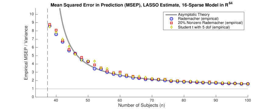
Figure 8.1. Universality of the LASSO Prediction Error. This plot shows the $\mathsf{MSEP}$ (8.2) obtained with the LASSO estimator (8.4), averaged over design matrices $\bm{X}$ and statistical errors $\bm{z}$. In the linear model (8.1), the number of predictors $p=64$; the number of active predictors $s=16$; each nonzero coefficient $(\bm{\beta}_{\star})_{j}$ in the model has unit magnitude; the statistical error $Z$ is Gaussian; the variance $\sigma^{2}=1$; and the number $n$ of subjects varies. The dashed line marks the location of the phase transition for the number of subjects required to identify the model exactly when the noise variance is zero. The gray curve delineates the asymptotic upper bound $n/(n-p\psi_{\ell_{1}}(s/p))$ for the normalized $\mathsf{MSEP}$ from Proposition 8.1. The markers give an empirical estimate (over 100 trials) for the $\mathsf{MSEP}$ when the design matrix $\bm{X}$ has the specified distribution.

8.2. Proof of Proposition 8.1

Without loss of generality, we may assume that the statistical model is scaled so the noise level $\sigma=1$. Define the sublevel set $E$ of the $\ell_{1}$ norm at the true parameter vector $\bm{\beta}_{\star}$:

$$E:=\big{\{}\bm{u}\in\mathbb{R}^{p}:\left\|{\smash{\bm{\beta}_{\star}+\bm{u}}}\right\|_{\ell_{1}}\leq\left\|{\smash{\bm{\beta}_{\star}}}\right\|_{\ell_{1}}\big{\}}.$$

Note that $E$ is a compact, convex set that contains the origin. Define the $n\times(p+1)$ random matrix $\bm{\Phi}:=\begin{bmatrix}\bm{X}&\bm{z}\end{bmatrix}$, and note that $\bm{\Phi}$ also follows Model 2.4. Making the change of variables $\bm{u}:=\bm{\beta}-\bm{\beta}_{\star}$, we can rewrite the LASSO problem (8.4) in the form

$$\underset{\bm{u}\in E}{\quad\text{minimize}\quad}\left\|{\bm{\Phi}\begin{bmatrix}\bm{u}\\ -1\end{bmatrix}}\right\|.$$ (8.6)

This expression depends on the assumption that $\sigma=1$. Let $\widehat{\bm{u}}$ be an optimal point of the problem (8.6). Referring to (8.3), we see that a formula for $\left\|{\widehat{\bm{u}}}\right\|^{2}$ leads to a formula for the $\mathsf{MSEP}$.

It will be helpful to introduce some additional sets. For a parameter $\alpha>0$, define the compact (but typically nonconvex) set

$$E_{\alpha}:=\big{\{}\bm{u}\in E:\left\|{\bm{u}}\right\|=\alpha\big{\}}.$$

We also define the compact and convex set

$$E_{\leq\alpha}:=\big{\{}\bm{u}\in E:\left\|{\bm{u}}\right\|\leq\alpha\big{\}}.$$

Observe that $E_{\alpha}\subset E_{\leq\alpha}$. Furthermore,

$$\alpha\leq\alpha_{+}\quad\text{implies}\quad(1/\alpha_{+})E_{\alpha_{+}}\subset(1/\alpha)E_{\alpha}.$$ (8.7)

The inclusion (8.7) holds because $E$ is convex and contains the origin.

Let $R_{\infty}$ be a constant that depends only on the parameters $\varrho$ and $\iota$. Suppose that $0\leq R\leq R_{+}\leq R_{\infty}$. To prove that $\left\|{\widehat{\bm{u}}}\right\|<R_{+}$, it suffices to establish the inequality

$$\min_{\bm{u}\in E_{\leq R}}\left\|{\bm{\Phi}\begin{bmatrix}\bm{u}\\ -1\end{bmatrix}}\right\|<\min_{\bm{u}\in E_{R_{+}}}\left\|{\bm{\Phi}\begin{bmatrix}\bm{u}\\ -1\end{bmatrix}}\right\|.$$ (8.8)

Indeed, recall that $\widehat{\bm{u}}$ is the minimizer of the objective over $E$, and let $\bm{u}_{0}$ be the point in $E_{\leq R}$ where the left-hand minimum in (8.8) is attained. The objective is a convex function of $\bm{u}$, so it does not decrease as $\bm{u}$ traverses the line segment from $\widehat{\bm{u}}$ to $\bm{u}_{0}$. If $\left\|{\widehat{\bm{u}}}\right\|\geq R_{+}$, this line segment muss pass through $E_{R_{+}}$, which is impossible because the ordering (8.8) forces the objective to decrease on the way from $E_{R_{+}}$ to $\bm{u}_{0}$.

Fix the parameter $R$ in the range $0\leq R\leq R_{\infty}$; we will select a suitable value later. Theorem II(b) demonstrates that, with high probability,

$$\min_{\bm{u}\in E_{\leq R}}\left\|{\bm{\Phi}\begin{bmatrix}\bm{u}\\ -1\end{bmatrix}}\right\|\leq\mathscr{E}_{n}\big{(}E_{\leq R}\times\{-1\}\big{)}+o(\sqrt{n})\leq\mathscr{E}_{n}\big{(}E_{R}\times\{-1\}\big{)}+o(\sqrt{n}).$$

The second relation holds because the excess width decreases with respect to set inclusion. Observe that

$$\mathscr{E}_{n}\big{(}E_{R}\times\{-1\}\big{)} =\operatorname{\mathbb{E}}\inf_{\bm{t}\in E_{R}}\big{(}\sqrt{n}(\left\|{\bm{t}}\right\|^{2}+1)^{1/2}+\bm{g}\cdot\bm{t}\big{)}$$

$$=\sqrt{n}(R^{2}+1)^{1/2}-\operatorname{\mathbb{E}}\sup_{\bm{t}\in E_{R}}\bm{g}\cdot\bm{t}$$

$$=\sqrt{n}(R^{2}+1)^{1/2}-R\,\mathscr{W}\big{(}(1/R)E_{R}\big{)}.$$

The last identity holds when we factor out $\left\|{\bm{t}}\right\|$ and identify the Gaussian width (3.7).

Fix the second parameter $R_{+}$, such that $R\leq R_{+}\leq R_{\infty}$. Theorem II(a) demonstrates that, with high probability,

$$\min_{\bm{u}\in E_{R_{+}}}\left\|{\bm{\Phi}\begin{bmatrix}\bm{u}\\ -1\end{bmatrix}}\right\|\geq\mathscr{E}_{n}\big{(}E_{R_{+}}\times\{-1\}\big{)}-o(\sqrt{n}).$$

Much as before, we calculate the excess width:

$$\mathscr{E}_{n}\big{(}E_{R_{+}}\times\{-1\}\big{)} =\sqrt{n}(R_{+}^{2}+1)^{1/2}-R_{+}\mathscr{W}\big{(}(1/R_{+})E_{R_{+}}\big{)}$$

$$\geq\sqrt{n}(R_{+}^{2}+1)^{1/2}-R_{+}\mathscr{W}\big{(}(1/R)E_{R}\big{)}.$$

The last inequality holds because of (8.7) and the fact that the Gaussian width is increasing with respect to set inclusion.

Combine the last four displays to reach

$$\min_{\bm{u}\in E_{\leq R}}\left\|{\bm{\Phi}\begin{bmatrix}\bm{u}\\ -1\end{bmatrix}}\right\| \leq\sqrt{n}(R^{2}+1)^{1/2}-R\,\mathscr{W}\big{(}(1/R)E_{R}\big{)}+o(\sqrt{n})$$

$$\leq\sqrt{n}(R_{+}^{2}+1)^{1/2}-R_{+}\mathscr{W}\big{(}(1/R)E_{R}\big{)}-o(\sqrt{n})\leq\min_{\bm{u}\in E_{R_{+}}}\left\|{\bm{\Phi}\begin{bmatrix}\bm{u}\\ -1\end{bmatrix}}\right\|.$$

It follows that we can establish (8.8) by finding parameters for which $0\leq R\leq R_{+}\leq R_{\infty}$ and

$$\left[\sqrt{n}(R_{+}^{2}+1)^{1/2}-R_{+}\mathscr{W}\big{(}(1/R)E_{R}\big{)}\right]-\left[\sqrt{n}(R^{2}+1)^{1/2}-R\,\mathscr{W}\big{(}(1/R)E_{R}\big{)}\right]\geq o(\sqrt{n}).$$

To that end, we replace the Gaussian width by a number that does not depend on the parameter $R$:

$$\mathscr{W}^{2}\big{(}(1/R)E_{R}\big{)}\leq\delta\big{(}(1/R)E_{R}\big{)}\leq\delta\big{(}\operatorname{cone}(E)\big{)}\leq p\psi_{\ell_{1}}(s/p)=:d.$$

The first relation is (3.8); the second follows from Definition 3.4; the last is the estimate (5.4). Moreover, these bounds are sharp when $R$ is sufficiently close to zero. Therefore, we just need to verify that

$$\left[\sqrt{n}(R_{+}^{2}+1)^{1/2}-R_{+}\sqrt{d}\right]-\left[\sqrt{n}(R^{2}+1)^{1/2}-R\,\sqrt{d}\right]\geq o(\sqrt{n}).$$ (8.9)

Once we choose $R$ and $R_{+}$ appropriately, we can adapt the analysis in the proof of Proposition 7.6.

For $\alpha\geq 0$, introduce the function

$$f(\alpha):=\sqrt{n}(\alpha^{2}+1)^{1/2}-\alpha\sqrt{d}.$$

As in the proof of Proposition 7.6, by direct calculation, $f$ is minimized at the value

$$R:=\frac{d}{n-d}.$$

Note that $R$ is very close to zero when $n\gg d$, in which case $d$ is an accurate bound for $\mathscr{W}^{2}\big{(}(1/R)E_{R}\big{)}$. Furthermore,

$$f(R)=\sqrt{n-d}.$$ (8.10)

Now, make the selection

$$R_{+}^{2}:=(1+\iota n/d)R^{2}=\frac{d+\iota n}{n-d}.$$ (8.11)

Since $n\geq(1+\varrho)\,d$, we see that $R_{+}$ is bounded by a constant $R_{\infty}$ that depends only on $\iota$ and $\varrho$. Repeating the calculation in (7.8), mutatis mutandis, we have

$$f(R_{+})\geq\frac{1+\iota/2}{\sqrt{1+\iota}}\sqrt{n-d}.$$ (8.12)

Combining (8.10) and (8.12), we determine that

$$f(R_{+})-f(R)\geq\frac{1+\iota/2-\sqrt{1+\iota}}{\sqrt{1+\iota}}\sqrt{n-d}\geq o(\sqrt{n}).$$

The last inequality holds because $\iota$ is a fixed positive constant and we have assumed that $n\geq(1+\varrho)d$.

In conclusion, we have confirmed the claim (8.9) for $R$ and the value $R_{+}$ designated in (8.11). It follows that (8.8) holds with high probability, and so the optimizer of (8.6) satisfies $\left\|{\widehat{\bm{u}}}\right\|\leq R_{+}$ with high probability. Therefore, the formula (8.2) for the mean squared error yields the bound

$$\mathsf{MSEP}=\left\|{\widehat{\bm{u}}}\right\|^{2}+1\leq R_{+}^{2}+1=(1+\iota)\frac{n}{n-d}.$$

Once again, we have used the assumption that $\sigma=1$. By homogeneity, the $\mathsf{MSEP}$ must be proportional to $\sigma^{2}$, which leads to the stated result (8.5). Finally, if we allow $\sigma\to 0$ with the other parameters fixed, the analysis here can be adapted to show that the error bound (8.5) is sharp.

Remark 8.2 (Prior Work).

In the special case of a standard normal design $\bm{X}$ and a standard normal error $\bm{z}$, the result of Proposition 8.1 appeared in the paper [OTH13]. Our extension to more general random models is new. Nevertheless, our proof has a lot in common with the analysis in [OTH13, TAH15].

Part III Universality of the Restricted Minimum Singular Value: Proofs of Theorem II and Theorem I(a)

In this part of the paper, we present a detailed proof of the universality law for the restricted singular value of a random matrix, Theorem II, and the first part of the universality law for the embedding dimension, Theorem I(a).

Section 9 contains our main technical result, which establishes universality for the bounded random matrix model, Model 2.1. Section 10 extends the result for bounded random matrices to the heavy-tailed random matrix model, Model 2.4. In Section 10.2, we obtain Theorem II as an immediate consequence of the result for heavy-tailed matrices. Section 10.3 shows how to derive Theorem I(a) as an additional consequence. The remaining sections in this part lay out the calculations that undergird the result for bounded random matrices.

9. The Restricted Singular Values of a Bounded Random Matrix

The key challenges in establishing universality for the restricted minimum singular value are already present in the case where the random matrix is drawn from the bounded model, Model 2.1. This section presents a universality law for bounded random matrices, and it gives an overview of the calculations that are required to establish this result.

9.1. Theorem 9.1: Main Result for the Bounded Random Matrix Model

The main technical result in this paper is a theorem on the behavior of the restricted minimum singular value of a bounded random matrix.

Theorem 9.1 (RSV: Bounded Random Matrix Model).

Place the following assumptions:

• Let $m$ and $n$ be natural numbers with $m\leq n^{6/5}$.

• Let $T$ be a closed subset of the unit ball $\mathsf{B}^{n}$ in $\mathbb{R}^{n}$.

• Draw an $m\times n$ random matrix $\bm{\Phi}$ from Model 2.1 with bound $B$.

Then the squared restricted singular value $\sigma_{\min}^{2}(\bm{\Phi};T)$ has the following properties:

1. The squared restricted singular value concentrates about its mean on a scale of $B^{2}\sqrt{m+n}$. For each $\zeta\geq 0$,

   $$\mathbb{P}\left\{{\sigma_{\min}^{2}(\bm{\Phi};T)\leq\operatorname{\mathbb{E}}\sigma_{\min}^{2}(\bm{\Phi};T)-\mathrm{C}B^{2}\zeta}\right\} \leq\mathrm{e}^{-\zeta^{2}/m},\quad\text{and}$$

   $$\mathbb{P}\left\{{\sigma_{\min}^{2}(\bm{\Phi};T)\geq\operatorname{\mathbb{E}}\sigma_{\min}^{2}(\bm{\Phi};T)+\mathrm{C}B^{2}\zeta}\right\} \leq\mathrm{C}\mathrm{e}^{-\zeta^{2}/(m+\zeta\sqrt{n})}.$$

2. The expectation of the squared restricted singular value is bounded below in terms of the excess width:

   $$\operatorname{\mathbb{E}}\sigma_{\min}^{2}(\bm{\Phi};T)\geq\big{(}\mathscr{E}_{m}(T)\big{)}_{+}^{2}-\mathrm{C}B^{2}(m+n)^{0.92}.$$

3. If $T$ is a convex set, the squared restricted singular value is bounded above in terms of the excess width:

   $$\operatorname{\mathbb{E}}\sigma_{\min}^{2}(\bm{\Phi};T)\leq\big{(}\mathscr{E}_{m}(T)\big{)}_{+}^{2}+\mathrm{C}B^{4}(m+n)^{0.94}.$$

Furthermore, the entries of $\bm{\Phi}$ need not be symmetric for this result to hold.

The proof of this result will occupy us for the rest of this part of the paper. This section summarizes the required calculations, with cross-references to the detailed arguments.

9.2. Proof of Theorem 9.1(1): Concentration

Theorem 9.1(1) states that the squared restricted singular value $\sigma_{\min}^{2}(\bm{\Phi};T)$ concentrates around its mean. We prove this claim in Proposition 11.1, which appears below. The argument depends on some concentration inequalities that are derived using the entropy method. This approach is more or less standard, so we move on to the more interesting part of the proof.

9.3. Setup for Proof of Theorem 9.1(2) and (3): Dissection of the Index Set

Let us continue with the proof of Theorem 9.1, conclusions (2) and (3). The overall approach is the same in both cases, but some of the details differ.

The first step is to dissect the index set $T$ into appropriate subsets. For each set $J\subset\{1,\dots,n\}$, we introduce a closed subset $T_{J}$ of $T$ via the rule

$$T_{J}:=\big{\{}\bm{t}\in T:\left|{\smash{t_{j}}}\right|\leq(\#J)^{-1/2}\text{ for all $j\in J^{c}$}\big{\}},$$ (9.1)

where $J^{c}:=\{1,\dots,n\}\setminus J$. In other words, $T_{J}$ contains all the vectors in $T$ where the coordinates listed in $J^{c}$ are sufficiently small. Note that convexity of the set $T$ implies convexity of each subset $T_{J}$.

Fix a number $k\in\{1,\dots,n\}$. Since $T$ is a subset of the unit ball $\mathsf{B}^{n}$, every vector $\bm{t}\in T$ satisfies

$$\#\big{\{}j:\left|{\smash{t_{j}}}\right|>k^{-1/2}\big{\}}\leq k.$$

Therefore, $\bm{t}$ belongs to some subset $T_{J}$ where the cardinality $\#J=k$, and we have the decomposition

$$T=\bigcup_{\#J=k}T_{J}.$$ (9.2)

It is clear that the number of subsets $T_{J}$ in this decomposition satisfies

$$\#\{T_{J}:\#J=k\}={n\choose k}\leq\left(\frac{\mathrm{e}n}{k}\right)^{k}.$$ (9.3)

We must limit the cardinality $k$ of the subsets, so we can control the number of subsets we need to examine.

9.4. Proof of Theorem 9.1(2): Lower Bound for the RSV

Let us proceed with the proof of Theorem 9.1(2), the lower bound for the RSV. For the time being, we fix the parameter $k$ that designates the cardinality of the sets $J$. We require that $k\geq m^{2/3}$.

First, we pass from the restricted singular value $\sigma_{\min}(\bm{\Phi};T)$ over the whole set $T$ to a bound that depends on $\sigma_{\min}(\bm{\Phi};T_{J})$ for the subsets $T_{J}$. Proposition 12.2 gives the comparison

$$\operatorname{\mathbb{E}}\sigma_{\min}^{2}(\bm{\Phi};T)\geq\min_{\#J=k}\operatorname{\mathbb{E}}\sigma_{\min}^{2}(\bm{\Phi};T_{J})-\mathrm{C}B^{2}\sqrt{km\log(n/k)}.$$ (9.4)

We have used the decomposition (9.2) and the bound (9.3) on the number of subsets in the decomposition to invoke the proposition. The main ingredient in the proof of this estimate is the concentration inequality for restricted singular values, Proposition 11.1.

Let us focus on a specific subset $T_{J}$. To study the restricted singular value $\sigma_{\min}(\bm{\Phi};T_{J})$, we want to replace the entries of the random matrix $\bm{\Phi}$ with standard normal random variables. Proposition 13.1 allows us to make partial progress toward this goal. Let $\bm{\Gamma}$ be an $m\times n$ standard normal matrix, independent from $\bm{\Phi}$. Define an $m\times n$ random matrix $\bm{\Psi}:=\bm{\Psi}(J)$ where $\bm{\Psi}_{J}=\bm{\Phi}_{J}$ and $\bm{\Psi}_{J^{c}}=\bm{\Gamma}_{J^{c}}$. Then

$$\operatorname{\mathbb{E}}\sigma_{\min}^{2}(\bm{\Phi};T_{J})\geq\operatorname{\mathbb{E}}\sigma_{\min}^{2}(\bm{\Psi};T_{J})-\frac{\mathrm{C}B^{2}m^{1/3}n\log(mn)}{k^{1/2}}.$$ (9.5)

This bound requires the assumption that $k\geq m^{2/3}$. The argument is based on the Lindeberg exchange principle, but we have used this method in an unusual way. For a vector $\bm{t}\in T_{J}$, the definition (9.1) gives us control on the magnitude of the entries listed in $J^{c}$, which we can exploit to replace the column submatrix $\bm{\Phi}_{J^{c}}$ with $\bm{\Gamma}_{J^{c}}$. The coordinates of $\bm{t}$ listed in $J$ may be large, so we cannot replace the column submatrix $\bm{\Phi}_{J}$ without incurring a significant penalty. Instead, we just leave it in place.

Next, we want to compare the expected RSV on the right-hand side of (9.5) with the excess width of the set $T_{J}$. Proposition 14.1 provides the bound

$$\operatorname{\mathbb{E}}\sigma_{\min}^{2}(\bm{\Psi};T_{J})\geq\left(\mathscr{E}_{m}(T_{J})-\mathrm{C}B^{2}\sqrt{k}\right)_{+}^{2}\geq\left(\mathscr{E}_{m}(T)-\mathrm{C}B^{2}\sqrt{k}\right)_{+}^{2}.$$ (9.6)

The second inequality is a consequence of the facts that $T_{J}\subset T$ and that the excess width is decreasing with respect to set inclusion. The calculation in Proposition 14.1 uses the Gaussian Minimax Theorem (see Fact A.3) to simplify the average with respect to the standard normal matrix $\bm{\Gamma}$. We also invoke standard results from nonasymptotic random matrix theory to control the expectation over $\bm{\Phi}_{J}$.

We can obtain a simple lower bound on the last term in (9.6) by linearizing the convex function $(\cdot)_{+}^{2}$ at the point $\mathscr{E}_{m}(T)$:

$$\left(\mathscr{E}_{m}(T)-\mathrm{C}B^{2}\sqrt{k}\right)_{+}^{2}\geq\big{(}\mathscr{E}_{m}(T)\big{)}_{+}^{2}-\mathrm{C}B^{2}\sqrt{k}\,\big{(}\mathscr{E}_{m}(T)\big{)}_{+}\geq\big{(}\mathscr{E}_{m}(T)\big{)}_{+}^{2}-\mathrm{C}B^{2}\sqrt{km}.$$ (9.7)

The last estimate follows from the observation that

$$\mathscr{E}_{m}(T)=\operatorname{\mathbb{E}}\inf_{\bm{t}\in T}\left(\sqrt{m}\left\|{\bm{t}}\right\|+\bm{g}\cdot\bm{t}\right)\leq\operatorname{\mathbb{E}}\left(\sqrt{m}\left\|{\bm{t}_{0}}\right\|+\bm{g}\cdot\bm{t}_{0}\right)\leq\sqrt{m}.$$ (9.8)

In this calculation, $\bm{t}_{0}$ is an arbitrary point in $T$.

Finally, we sequence the four displays (9.4), (9.5), (9.6), and (9.7) and combine error terms to obtain

$$\operatorname{\mathbb{E}}\sigma_{\min}^{2}(\bm{\Phi};T)\geq\big{(}\mathscr{E}_{m}(T)\big{)}_{+}^{2}-\frac{\mathrm{C}B^{2}m^{1/3}n\log(mn)}{k^{1/2}}-\mathrm{C}B^{2}\sqrt{km\log(n/k)}.$$ (9.9)

Up to logarithms, an optimal choice of the cardinality parameter is $k=\lceil m^{-1/6}n\rceil$. Since $m\leq n^{6/5}$, this choice ensures that $k\geq m^{2/3}$. We conclude that

$$\operatorname{\mathbb{E}}\sigma_{\min}^{2}(\bm{\Phi};T) \geq\big{(}\mathscr{E}_{m}(T)\big{)}_{+}^{2}-\mathrm{C}B^{2}m^{5/12}n^{1/2}\log(mn)$$

$$\geq\big{(}\mathscr{E}_{m}(T)\big{)}_{+}^{2}-\mathrm{C}B^{2}(m+n)^{11/12}\log(m+n).$$

Combine the logarithm with the power, and adjust the constants to complete the proof of Theorem 9.1(2).

9.5. Proof of Theorem 9.1(3): Upper Bound for the RSV of a Convex Set

At a high level, the steps in the proof of Theorem 9.1(3) are similar with the argument in the last section. Many of the technical details, however, depend on convex duality arguments.

As before, we fix the cardinality parameter $k$, with the requirement $k\geq m^{2/3}$. The first step is to pass from $\sigma_{\min}(\bm{\Phi};T)$ to $\sigma_{\min}(\bm{\Phi};T_{J})$. We have

$$\operatorname{\mathbb{E}}\sigma_{\min}^{2}(\bm{\Phi};T)\leq\min_{\#J=k}\operatorname{\mathbb{E}}\sigma_{\min}^{2}(\bm{\Phi};T_{J}).$$ (9.10)

This bound is a trivial consequence of the facts that $T_{J}\subset T$ for each subset $J$ of $\{1,\dots,n\}$ and that $\sigma_{\min}(\bm{\Phi};\cdot)$ is decreasing with respect to set inclusion.

Select any subset $T_{J}$. We invoke Proposition 13.1 to exchange most of the entries of the random matrix $\bm{\Phi}$ for standard normal variables. Using the same random matrix $\bm{\Psi}$ from the last section, we have

$$\operatorname{\mathbb{E}}\sigma_{\min}^{2}(\bm{\Phi};T_{J})\leq\operatorname{\mathbb{E}}\sigma_{\min}^{2}(\bm{\Psi};T_{J})+\frac{\mathrm{C}B^{2}m^{1/3}n\log(mn)}{k^{1/2}}.$$ (9.11)

The bound (9.11) requires the assumption $k\geq m^{2/3}$, and the proof is identical with the proof of the lower bound (9.5).

Next, we compare the expected RSV on the right-hand side of (9.11) with the excess width. Proposition 14.1 delivers

$$\operatorname{\mathbb{E}}\sigma_{\min}^{2}(\bm{\Psi};T_{J})\leq\left(\mathscr{E}_{m}(T_{J})+\mathrm{C}B^{2}\sqrt{k}\right)_{+}^{2}.$$ (9.12)

This argument is more complicated than the analogous lower bound (9.6), and it depends on the convexity of $T_{J}$. We also apply the assumption that $k\geq m^{2/3}$ here.

Proposition 12.1 allows us to replace the excess width of $T_{J}$ in (9.12) with the excess width of $T$:

$$\mathscr{E}_{m}(T_{J})\leq\mathscr{E}_{m}(T)+\mathrm{C}\sqrt{k\log(n/k)}.$$ (9.13)

We use the decomposition (9.2) and the bound (9.3) on the number of sets $T_{J}$ to invoke the proposition. This proof depends on the Gaussian concentration inequality.

Sequence the bounds (9.10), (9.11), (9.12), and (9.13), and combine the error terms to arrive at

$$\operatorname{\mathbb{E}}\sigma_{\min}^{2}(\bm{\Phi};T)\leq\left(\mathscr{E}_{m}(T)+\mathrm{C}B^{2}\sqrt{k\log(n/k)}\right)_{+}^{2}+\frac{\mathrm{C}B^{2}m^{1/3}n\log(mn)}{k^{1/2}}.$$

Expand the square using (9.8) to reach

$$\operatorname{\mathbb{E}}\sigma_{\min}^{2}(\bm{\Phi};T)\leq\big{(}\mathscr{E}_{m}(T)\big{)}_{+}^{2}+\mathrm{C}B^{2}\left(\frac{m^{1/3}n\log(mn)}{k^{1/2}}+\sqrt{km\log(n/k)}+B^{2}k\log(n/k)\right).$$

Select $k=\lceil n^{4/5}\rceil$ to arrive at

$$\operatorname{\mathbb{E}}\sigma_{\min}^{2}(\bm{\Phi};T) \leq\big{(}\mathscr{E}_{m}(T)\big{)}_{+}^{2}+\mathrm{C}B^{2}(m^{1/3}n^{3/5}+n^{2/5}m^{1/2})\log(n)+\mathrm{C}B^{4}n^{4/5}\log(mn)$$

$$\leq\big{(}\mathscr{E}_{m}(T)\big{)}_{+}^{2}+\mathrm{C}B^{4}(m+n)^{14/15}\log(m+n).$$

Combine the power with the logarithm, and adjust constants to finish the proof of Theorem 9.1(3).

10. The Restricted Singular Values of a Heavy-Tailed Random Matrix

In this section, we present an extension of Theorem 9.1 to the heavy-tailed matrix model, Model 2.4. In Section 10.2, we explain how the universality result for the restricted singular value, Theorem II, is an immediate consequence. In Section 10.3, we show how to derive the first half of the universality result for the embedding dimension, Theorem I(a).

10.1. Corollary 10.1: Main Result for the $p$-Moment Random Matrix Model

We can extend Theorem 9.1 to the heavy-tailed random matrix model, Model 2.4 using a truncation argument. The following corollary contains a detailed statement of the result.

Corollary 10.1 (RSV: $p$-Moment Random Matrix Model).

Fix parameters $p>4$ and $\nu\geq 1$. Place the following assumptions:

• Let $m$ and $n$ be natural numbers with $m\leq n^{6/5}$.

• Let $T$ be a closed subset of the unit ball $\mathsf{B}^{n}$ in $\mathbb{R}^{n}$.

• Draw an $m\times n$ random matrix $\bm{\Phi}$ that satisfies Model 2.4 with given $p$ and $\nu$.

Then the restricted singular value $\sigma_{\min}(\bm{\Phi};T)$ has the following properties:

1. With high probability, the restricted singular value is bounded below by the excess width:

   $$\mathbb{P}\left\{{\sigma_{\min}(\bm{\Phi};T)\leq\big{(}\mathscr{E}_{m}(T)\big{)}_{+}-\mathrm{C}_{p}\nu(m+n)^{1/2-\kappa(p)}}\right\}\leq\mathrm{C}_{p}(m+n)^{1-p/4}.$$ (10.1)

2. If $T$ is a convex set, with high probability, the restricted singular value is bounded above by the excess width:

   $$\mathbb{P}\left\{{\sigma_{\min}(\bm{\Phi};T)\geq\big{(}\mathscr{E}_{m}(T)\big{)}_{+}+\mathrm{C}_{p}\nu^{2}(m+n)^{1/2-\kappa(p)}}\right\}\leq\mathrm{C}_{p}(m+n)^{1-p/4}.$$ (10.2)

The function $\kappa(p)$ is strictly positive for $p>4$, and the constant $\mathrm{C}_{p}$ depends only on $p$.

The proof of Corollary 10.1 appears below in Section 15. The main idea is to truncate each entry of the heavy-tailed random matrix $\bm{\Phi}$ individually. We can treat the bounded part of the random matrix using Theorem 9.1. We show that the tails are negligible by means of a relatively simple norm bound for random matrices, Fact B.2.

10.2. Proof of Theorem II from Corollary 10.1

Theorem II is an easy consequence of Corollary 10.1. Recall the assumptions of the theorem:

• The embedding dimension satisfies $\lambda D\leq d\leq D^{6/5}$.

• $E$ is a closed subset of the unit ball in $\mathbb{R}^{D}$.

• The $d$-excess width of $E$ satisfies $\mathscr{E}_{d}(E)\geq\varrho\sqrt{d}$.

• The $d\times D$ random linear map $\bm{\Pi}$ follows Model 2.4 with parameters $p>4$ and $\nu\geq 1$.

Therefore, we may apply Corollary 10.1 with $\bm{\Phi}=\bm{\Pi}$ and $T=E$ to see that

$$\mathbb{P}\left\{{\sigma_{\min}(\bm{\Pi};E)\leq\big{(}\mathscr{E}_{d}(E)\big{)}_{+}-\mathrm{C}_{p}\nu(d+D)^{1/2-\kappa(p)}}\right\} \leq\mathrm{C}_{p}D^{1-p/4},\quad\text{and}$$

$$\mathbb{P}\left\{{\sigma_{\min}(\bm{\Pi};E)\geq\big{(}\mathscr{E}_{d}(E)\big{)}_{+}+\mathrm{C}_{p}\nu^{2}(d+D)^{1/2-\kappa(p)}}\right\} \leq\mathrm{C}_{p}D^{1-p/4}\phantom{,}\quad\text{if $E$ is convex.}$$

For simplicity, we have dropped the embedding dimension $d$ from the right-hand side of the bounds in the last display.

To prove Theorem II, it suffices to check that we can make the error term $\mathrm{C}_{p}\nu^{2}(d+D)^{1/2-\kappa(p)}$ smaller than $\varepsilon\mathscr{E}_{d}(E)$ if we select the ambient dimension $D$ large enough. Indeed, the conditions $D\leq\lambda^{-1}d$ and $d^{1/2}\leq\varrho^{-1}\mathscr{E}_{d}(E)$ ensure that

$$(d+D)^{1/2-\kappa(p)} \leq(1+\lambda^{-1})^{1/2}d^{1/2-\kappa(p)}$$

$$\leq(1+\lambda^{-1})^{1/2}\varrho^{-1}\mathscr{E}_{d}(E)d^{-\kappa(p)}$$

$$\leq\frac{(1+\lambda^{-1})^{1/2}\varrho^{-1}\lambda^{-\kappa(p)}}{D^{\kappa(p)}}\mathscr{E}_{d}(E)$$

Since $\kappa(p)$ is positive, there is a number $N:=N(p,\nu,\lambda,\varrho,\varepsilon)$ for which $D\geq N$ implies

$$\mathrm{C}_{p}\nu^{2}(d+D)^{1/2-\kappa(p)}\leq\varepsilon\mathscr{E}_{d}(E).$$

This is what we needed to show.

10.3. Proof of Theorem I(a) from Corollary 10.1

Theorem I(a) is also an easy consequence of Corollary 10.1. Recall the assumptions of the theorem:

• $E$ is a compact subset of $\mathbb{R}^{D}$ that does not contain the origin.

• The statistical dimension of $E$ satisfies $\delta(E)\geq\varrho D$.

• The $d\times D$ random linear map $\bm{\Pi}$ follows Model 2.4 with parameters $p>4$ and $\nu\geq 1$.

In this section, we consider the regime where the embedding dimension $d\geq(1+\varepsilon)\,\delta(E)$. We need to demonstrate that

$$\mathbb{P}\left\{{\bm{0}\notin\bm{\Pi}(E)}\right\}=\mathbb{P}\left\{{E\cap\operatorname{null}(\bm{\Pi})=\emptyset}\right\}\geq 1-\mathrm{C}_{p}D^{1-p/4}.$$ (10.3)

We begin with a reduction to a specific choice of the embedding dimension $d$. Let $\bm{\Pi}_{m}$ be the $m\times D$ matrix formed from the first $m$ rows of the random linear map $\bm{\Pi}$. The function $m\mapsto\mathbb{P}\left\{{E\cap\operatorname{null}(\bm{\Pi}_{m})=\emptyset}\right\}$ is weakly increasing because $m\mapsto\operatorname{null}(\bm{\Pi}_{m})$ is a decreasing sequence of sets. Therefore, it suffices to verify (10.3) in the case where $d=\lceil(1+\varepsilon)\,\delta(E)\rceil$. Note that $d\leq 2D+1$ because the statistical dimension $\delta(E)\leq D$ and $\varepsilon<1$.

Introduce the spherical retraction $\Omega:=\bm{\theta}(E)$. Proposition 3.8 and (3.2) demonstrate that

$$\sigma_{\min}(\bm{\Pi};\Omega)>0\quad\text{implies}\quad\bm{0}\notin\bm{\Pi}(\Omega)\quad\text{implies}\quad\bm{0}\notin\bm{\Pi}(E).$$

Therefore, to check (10.3), it suffices to produce a high-probability lower bound on the restricted singular value $\sigma_{\min}(\bm{\Pi};\Omega)$. With the choices $\bm{\Phi}=\bm{\Pi}$ and $T=\Omega$, Corollary 10.1 yields

$$\mathbb{P}\left\{{\sigma_{\min}(\bm{\Pi};\Omega)\geq\big{(}\mathscr{E}_{d}(\Omega)\big{)}_{+}-\mathrm{C}_{p}\nu(d+D)^{1/2-\kappa(p)}}\right\}\geq 1-\mathrm{C}_{p}D^{1-p/4}.$$

To complete the proof, we need to verify that our hypotheses imply

$$\mathscr{E}_{d}(\Omega)>\mathrm{C}_{p}\nu(d+D)^{1/2-\kappa(p)}.$$ (10.4)

This point follows from two relatively short calculations.

Since $\Omega$ is a subset of the unit sphere, we quickly compute ite excess width:

$$\mathscr{E}_{d}(\Omega)=\operatorname{\mathbb{E}}\inf_{\bm{x}\in\Omega}\big{(}\sqrt{d}\left\|{\bm{x}}\right\|+\bm{g}\cdot\bm{x}\big{)} \geq\sqrt{d}-\sqrt{\delta(\Omega)}$$ (10.5)

$$=\sqrt{d}-\sqrt{\delta(E)}\geq\big{(}\sqrt{1+\varepsilon}-1\big{)}\sqrt{\delta(E)}.$$

The second identity holds because $\Omega$ is a subset of the unit sphere, and we have used the relation (4.3). Recall that the statistical dimension of a general set $E$ is defined as $\delta(E)=\delta(\bm{\theta}(E))$, and then introduce the value $d=\lceil(1+\varepsilon)\,\delta(E)\rceil$ of the embedding dimension.

Meanwhile, we can bound the dimensional term in (10.4) above:

$$(d+D)^{1/2-\kappa(p)}\leq\mathrm{C}D^{1/2-\kappa(p)}\leq\mathrm{C}\varrho^{-1/2}D^{-\kappa(p)}\sqrt{\delta(E)}.$$

The first inequality holds because $d\leq 2D+1$, and the second inequality uses the assumption $D\leq\varrho^{-1}\delta(E)$. Since $\kappa(p)$ is positive, we can find a number $N:=N(p,\nu,\varrho,\varepsilon)$ for which $D\geq N$ implies that

$$\mathrm{C}_{p}\nu(d+D)^{1/2-\kappa(p)}<\big{(}\sqrt{1+\varepsilon}-1\big{)}\sqrt{\delta(E)}.$$

Combine the last display with (10.5) to determine that the claim (10.4) is valid.

11. Theorem 9.1: Concentration for Restricted Singular Values

In this section, we demonstrate that the restricted minimum singular value of a bounded random matrix concentrates about its mean value. This result yields Theorem 9.1(1).

Proposition 11.1 (Theorem 9.1: Concentration).

Let $S$ be a closed subset of $\mathsf{B}^{n}$. Let $\bm{\Phi}$ be an $m\times n$ random matrix drawn from Model 2.1 with uniform bound $B$. For all $\zeta\geq 0$,

$$\mathbb{P}\left\{{\sigma_{\min}^{2}(\bm{\Phi};S)\leq\operatorname{\mathbb{E}}\sigma_{\min}^{2}(\bm{\Phi};S)-\mathrm{C}B^{2}\zeta}\right\} \leq\mathrm{e}^{-\zeta^{2}/m}$$ (11.1)

$$\mathbb{P}\left\{{\sigma_{\min}^{2}(\bm{\Phi};S)\geq\operatorname{\mathbb{E}}\sigma_{\min}^{2}(\bm{\Phi};S)+\mathrm{C}B^{2}\zeta}\right\} \leq\mathrm{e}^{-\zeta^{2}/(m+\zeta\sqrt{n})}.$$ (11.2)

The proof relies on some modern concentration inequalities that are derived using the entropy method. We establish the bound (11.1) on the lower tail in Section 11.1; the bound (11.2) on the upper tail appears in Section 11.2.

In several other parts of the paper, we rely on variants of Proposition 11.1 that follow from essentially the same arguments. We omit the details of these proofs to avoid repetition.

11.1. Proposition 11.1: The Lower Tail of the RSV

First, we establish that the restricted singular value is unlikely to be much smaller than its mean. The proof depends on an exponential moment inequality derived using Massart’s modified logarithmic Sobolev inequality [Mas00]. For instance, see [BLM13, Thm. 6.27] or [Mau12, Thm. 19].

Fact 11.2 (Self-Bounded Random Variable: Lower Tail).

Let $(X_{1},\dots,X_{p})$ be an independent sequence of real random variables. For a nonnegative function $f:\mathbb{R}^{p}\to\mathbb{R}_{+}$, define

$$Y := f(X_{1},\dots,X_{i-1},X_{i},X_{i+1},\dots,X_{p}),\quad\text{and}$$

$$\sup\nolimits_{i}Y :=\sup_{\alpha\in\operatorname{supp}(X_{i})} f(X_{1},\dots,X_{i-1},\alpha,X_{i+1},\dots,X_{p})\quad\text{for $i=1,\dots,p$.}$$

Suppose that

$$\Delta_{-}:=\sum_{i=1}^{p}\big{(}\sup\nolimits_{i}Y-Y\big{)}^{2}\leq aY+b\quad\text{where $a,b\geq 0$.}$$

Then, for $\zeta\geq 0$,

$$\mathbb{P}\left\{{Y\leq\operatorname{\mathbb{E}}Y-\zeta}\right\}\leq\exp\left(\frac{-\zeta^{2}/2}{a\operatorname{\mathbb{E}}Y+b}\right).$$

The function $\operatorname{supp}(\cdot)$ returns the support of a random variable.

With this fact at hand, we may derive the lower tail bound.

Proof of Proposition 11.1, Eqn. (11.1).

Introduce the random variable

$$Y:=\sigma_{\min}^{2}(\bm{\Phi};S)=\min_{\bm{s}\in S}\left\|{\bm{\Phi}\bm{s}}\right\|^{2}=\min_{\bm{s}\in S}\sum_{i=1}^{m}\left(\sum_{j=1}^{n}\varphi_{ij}s_{j}\right)^{2}.$$

For each index pair $(i,j)$ and real number $\alpha$, define a random matrix $\bm{\Phi}_{\alpha}^{(ij)}$ by replacing the $(i,j)$ entry $\varphi_{ij}$ of $\bm{\Phi}$ with the number $\alpha$. Now, the random variable

$$\sup\nolimits_{ij}Y=\max_{\left|{\alpha}\right|\leq B}\sigma_{\min}^{2}\big{(}\bm{\Phi}^{(ij)}_{\alpha};S\big{)}=\max_{\left|{\alpha}\right|\leq B}\min_{\bm{s}\in S}\left\|{\smash{\bm{\Phi}^{(ij)}_{\alpha}\bm{s}}}\right\|^{2}.$$

We must evaluate the lower variance proxy

$$\Delta_{-}:=\sum_{i=1}^{m}\sum_{j=1}^{n}\big{(}\sup\nolimits_{ij}Y-Y\big{)}^{2}.$$

To that end, select a point $\bm{t}\in\operatorname*{arg\;min}_{\bm{s}\in S}\left\|{\bm{\Phi}\bm{s}}\right\|^{2}$. For each index pair $(i,j)$,

$$\sup\nolimits_{ij}Y-Y=\max_{\left|{\alpha}\right|\leq B}\min_{\bm{s}\in S}\left\|{\smash{\bm{\Phi}^{(ij)}_{\alpha}}\bm{s}}\right\|^{2}-\min_{\bm{s}\in S}\left\|{\bm{\Phi}\bm{s}}\right\|^{2}\leq\max_{\left|{\alpha}\right|\leq B}\left\|{\smash{\bm{\Phi}^{(ij)}_{\alpha}\bm{t}}}\right\|^{2}-\left\|{\bm{\Phi}\bm{t}}\right\|^{2}.$$

The matrix $\bm{\Phi}^{(ij)}_{\alpha}$ differs from $\bm{\Phi}$ only in the $i$th row. Therefore, when we expand the squared norms into components, all of the components cancel except for the $i$th one. We discover that

$$\sup\nolimits_{ij}Y-Y \leq\max_{\left|{\alpha}\right|\leq B}\left(\big{(}(\alpha-\varphi_{ij})t_{j}+\sum_{\ell=1}^{n}\varphi_{i\ell}t_{\ell}\big{)}^{2}-\big{(}\sum_{\ell=1}^{n}\varphi_{i\ell}t_{\ell}\big{)}^{2}\right)$$ (11.3)

$$=\max_{\left|{\alpha}\right|\leq B}\left((\alpha-\varphi_{ij})^{2}t_{j}^{2}+2(\alpha-\varphi_{ij})t_{j}\sum_{\ell=1}^{n}\varphi_{i\ell}t_{\ell}\right)$$

$$\leq\max_{\left|{\alpha}\right|\leq B}\left((\alpha-\varphi_{ij})^{2}t_{j}^{2}+2\left|{\smash{\alpha-\varphi_{ij}}}\right|\left|{\smash{t_{j}}}\right|\left|{\sum_{\ell=1}^{n}\varphi_{i\ell}t_{\ell}}\right|\right)$$

$$\leq 4B^{2}t_{j}^{2}+4B\left|{\smash{t_{j}}}\right|\left|{\sum_{\ell=1}^{n}\varphi_{i\ell}t_{\ell}}\right|.$$

The last inequality holds because $\left|{\alpha}\right|\leq B$ and $\left|{\smash{\varphi_{ij}}}\right|\leq B$. As a consequence,

$$\big{(}\sup\nolimits_{ij}Y-Y\big{)}^{2}\leq\left(4B^{2}t_{j}^{2}+4B\left|{\smash{t_{j}}}\right|\left|{\sum_{\ell=1}^{n}\varphi_{i\ell}t_{\ell}}\right|\right)^{2}\leq 32B^{4}t_{j}^{4}+32B^{2}t_{j}^{2}\left(\sum_{\ell=1}^{n}\varphi_{i\ell}t_{\ell}\right)^{2}.$$

Sum over pairs $(i,j)$ to arrive at

$$\sum_{i=1}^{m}\sum_{j=1}^{n}\big{(}\sup\nolimits_{ij}Y-Y\big{)}^{2} \leq\sum_{i=1}^{m}\sum_{j=1}^{n}\left(32B^{4}t_{j}^{4}+32B^{2}t_{j}^{2}\left(\sum_{\ell=1}^{n}\varphi_{i\ell}t_{\ell}\right)^{2}\right)$$

$$\leq 32B^{4}m+32B^{2}\sum_{i=1}^{m}\left(\sum_{\ell=1}^{n}\varphi_{i\ell}t_{\ell}\right)^{2}$$

$$=32B^{4}m+32B^{2}\left\|{\bm{\Phi}\bm{t}}\right\|^{2}$$

$$=32B^{4}m+32B^{2}\min_{\bm{s}\in S}\left\|{\bm{\Phi}\bm{s}}\right\|^{2}.$$

To reach the second line, we used the fact that $\left\|{\bm{t}}\right\|_{\ell_{4}}\leq\left\|{\bm{t}}\right\|\leq 1$. The last line depends on the definition of $\bm{t}$.

In summary, we have demonstrated that

$$\Delta_{-}\leq 32B^{2}Y+32B^{4}m.$$

To apply Fact 11.2, we need a bound for the expectation of $Y$. Designate a point $\bm{s}_{0}\in S$, and calculate that

$$\operatorname{\mathbb{E}}Y\leq\operatorname{\mathbb{E}}\left\|{\bm{\Phi}\bm{s}_{0}}\right\|^{2}=m\left\|{\bm{s}_{0}}\right\|^{2}\leq m.$$

The identity holds because $\bm{\Phi}$ has independent, standardized entries. Fact 11.2 ensures that

$$\mathbb{P}\left\{{Y\leq\operatorname{\mathbb{E}}Y-\zeta}\right\}\leq\exp\left(\frac{-\zeta^{2}/2}{32B^{2}\operatorname{\mathbb{E}}Y+32B^{4}m}\right)\leq\exp\left(\frac{-\zeta^{2}}{128B^{4}m}\right).$$

Rewrite this formula to complete the proof of (11.1). ∎

11.2. Proposition 11.1: The Upper Tail of the RSV

Next, we establish that the restricted singular value of a bounded random matrix is unlikely to be much larger than its mean. The proof depends on another tail inequality for self-bounded random variables. This result also follows from Massart’s modified log-Sobolev inequality [Mas00]; the argument is similar to the proofs of [Mau12, Thms. 18, 19]

Fact 11.3 (Self-Bounded Random Variable: Upper Tail).

Let $(X_{1},\dots,X_{p})$ be an independent sequence of real random variables. For a function $f:\mathbb{R}^{p}\to\mathbb{R}$, define

$$Y := f(X_{1},\dots,X_{i-1},X_{i},X_{i+1},\dots,X_{p}),\quad\text{and}$$

$$\sup\nolimits_{i}Y :=\sup_{\alpha\in\operatorname{supp}(X_{i})} f(X_{1},\dots,X_{i-1},\alpha,X_{i+1},\dots,X_{p})\quad\text{for $i=1,\dots,p$.}$$

Suppose that $\sup_{i}Y-Y\leq L$ uniformly for a fixed value $L$ and that

$$\Delta_{-}:=\sum_{i=1}^{p}\big{(}\sup\nolimits_{i}Y-Y\big{)}^{2}\leq aY+b\quad\text{where $a,b\geq 0$.}$$

Then, for $\zeta\geq 0$,

$$\mathbb{P}\left\{{Y\geq\operatorname{\mathbb{E}}Y+\zeta}\right\}\leq\exp\left(\frac{-\zeta^{2}/2}{(a\operatorname{\mathbb{E}}Y+b)+(a+L)\zeta}\right).$$

The function $\operatorname{supp}(\cdot)$ returns the support of a random variable.

Proof of Proposition 11.1, Eqn. (11.2).

We proceed as in the proof of (11.1). It just remains to verify the uniform bound on $\sup_{ij}Y-Y$. Starting from (11.3), we calculate that

$$\sup\nolimits_{ij}Y-Y \leq 4B^{2}t_{j}^{2}+4B\left|{\smash{t_{j}}}\right|\left|{\sum_{\ell=1}^{n}\varphi_{il}t_{\ell}}\right|$$

$$\leq 4B^{2}+4B\left(\sum_{\ell=1}^{n}\varphi_{i\ell}^{2}\right)^{1/2}$$

$$\leq 4B^{2}+4B^{2}\sqrt{n}$$

$$\leq 8B^{2}\sqrt{n}.$$

This calculation relies on the fact that $\left\|{\bm{t}}\right\|\leq 1$ and the entries of $\bm{\Phi}$ have magnitude bounded by $B$. Apply Fact 11.3 to complete the argument. ∎

12. Theorem 9.1: Probability Bounds for Dissections

In this section, we establish some results that compare the expectation of a minimum of random variables indexed by a set with the expectations of the minima indexed by subsets. These facts are easy consequences of concentration phenomena.

12.1. Dissection of the Excess Width

First, we show that the excess width of a set can be related to the excess width of a collection of subsets.

Proposition 12.1 (Theorem 9.1: Dissection of Excess Width).

Consider a closed subset $T$ of the unit ball $\mathsf{B}^{n}$ that has been decomposed into a finite number of closed subsets $T_{J}$:

$$T=\bigcup_{J\in\mathscr{J}}T_{J}.$$

For each $m\geq 0$, it holds that

$$\bigg{(}\operatorname{\mathbb{E}}\min_{\bm{t}\in T}\big{(}\sqrt{m}\left\|{\bm{t}}\right\|+\bm{g}\cdot\bm{t}\big{)}\bigg{)}_{+}\geq\min_{J\in\mathscr{J}}\operatorname{\mathbb{E}}\min_{\bm{t}\in T_{J}}\big{(}\sqrt{m}\left\|{\bm{t}}\right\|+\bm{g}\cdot\bm{t}\big{)}-\mathrm{C}\sqrt{\log(\#\mathscr{J})}.$$

In other words,

$$\min_{J\in\mathscr{J}}\big{(}\mathscr{E}_{m}(T_{J})\big{)}_{+}\leq\big{(}\mathscr{E}_{m}(T)\big{)}_{+}+\mathrm{C}\sqrt{\log(\#\mathscr{J})}.$$

Proof.

Since $T=\bigcup_{J\in\mathscr{J}}T_{J}$, we can stratify the minimum over $T$:

$$\min_{\bm{t}\in T}\big{(}\sqrt{m}\left\|{\bm{t}}\right\|+\bm{g}\cdot\bm{t}\big{)}=\min_{J\in\mathscr{J}}\min_{\bm{t}\in T_{J}}\big{(}\sqrt{m}\left\|{\bm{t}}\right\|+\bm{g}\cdot\bm{t}\big{)}.$$

We will obtain a lower tail bound for the minimum over $T$ by combining lower tail bounds for each minimum over $T_{J}$. Then we integrate the tail probability to obtain the required expectation bound.

Each subset $T_{J}$ is contained in $\mathsf{B}^{n}$, so the map

$$\bm{g}\mapsto\min_{\bm{t}\in T_{J}}\big{(}\sqrt{m}\left\|{\bm{t}}\right\|+\bm{g}\cdot\bm{t}\big{)}$$

is 1-Lipschitz. The Gaussian concentration inequality, Fact A.2, provides a tail bound. For each $J\in\mathscr{J}$ and for each $\lambda\geq 0$,

$$\mathbb{P}\left\{{\min_{\bm{t}\in T_{J}}\big{(}\sqrt{m}\left\|{\bm{t}}\right\|+\bm{g}\cdot\bm{t}\big{)}\leq\operatorname{\mathbb{E}}\min_{\bm{t}\in T_{J}}\big{(}\sqrt{m}\left\|{\bm{t}}\right\|+\bm{g}\cdot\bm{t}\big{)}-\lambda}\right\}\leq\mathrm{e}^{-\lambda^{2}/2}.$$

Apply the union bound over $J\in\mathscr{J}$ to see that, for all $\zeta\geq 0$,

$$\mathbb{P}\left\{{\min_{\bm{t}\in T}\big{(}\sqrt{m}\left\|{\bm{t}}\right\|+\bm{g}\cdot\bm{t}\big{)}\leq\min_{J\in\mathscr{J}}\operatorname{\mathbb{E}}\min_{\bm{t}\in T_{J}}\big{(}\sqrt{m}\left\|{\bm{t}}\right\|+\bm{g}\cdot\bm{t}\big{)}-\sqrt{2\log(\#\mathscr{J})}-\zeta}\right\}\\ \leq(\#\mathscr{J})\mathrm{e}^{-(\sqrt{2\log(\#\mathscr{J})}+\zeta)^{2}/2}\leq\mathrm{e}^{-\zeta^{2}/2}.$$

Using the latter estimate, we quickly compute the excess width of $T$. Abbreviate

$$Y:=\min_{\bm{t}\in T}\big{(}\sqrt{m}\left\|{\bm{t}}\right\|+\bm{g}\cdot\bm{t}\big{)}\quad\text{and}\quad\alpha:=\min_{J\in\mathscr{J}}\operatorname{\mathbb{E}}\min_{\bm{t}\in T_{J}}\big{(}\sqrt{m}\left\|{\bm{t}}\right\|+\bm{g}\cdot\bm{t}\big{)}-\sqrt{2\log(\#\mathscr{J})}.$$

If $\alpha\leq 0$, the stated result is trivial, so we may assume that $\alpha>0$. The integration by parts representation of the expectation yields

$$(\operatorname{\mathbb{E}}Y)_{+}\geq\int_{0}^{\alpha}\mathbb{P}\left\{{Y>\zeta}\right\}\,\mathrm{d}{\zeta}=\int_{0}^{\alpha}\mathbb{P}\left\{{Y>\alpha-\zeta}\right\}\,\mathrm{d}{\zeta}=\alpha-\int_{0}^{\alpha}\mathbb{P}\left\{{Y\leq\alpha-\zeta}\right\}\,\mathrm{d}{\zeta}\geq\alpha-\int_{0}^{\alpha}\mathrm{e}^{-\zeta^{2}/2}\,\mathrm{d}{\zeta}>\alpha-\sqrt{\pi/2}.$$

Reintroduce the values of $Y$ and $\alpha$, and combine constants to complete the argument. ∎

12.2. Dissection of the Restricted Singular Value

Next, we show that the minimum singular value of a random matrix, restricted to a set, is controlled by the minimum singular value, restricted to subsets.

Proposition 12.2 (Theorem 9.1: Dissection of RSV).

Consider a closed subset $T$ of the unit ball $\mathsf{B}^{n}$, and assume that it has been decomposed into a finite number of closed subsets $T_{J}$:

$$T=\bigcup_{J\in\mathscr{J}}T_{J}.$$

Let $\bm{\Phi}$ be an $m\times n$ random matrix that satisfies Model 2.1 with uniform bound $B$. Then

$$\min_{J\in\mathscr{J}}\operatorname{\mathbb{E}}\sigma_{\min}^{2}(\bm{\Phi};T_{J})\leq\operatorname{\mathbb{E}}\sigma_{\min}^{2}(\bm{\Phi};T)+\mathrm{C}B^{2}\sqrt{m\log(\#\mathscr{J})}.$$

Proof.

The argument is similar with the proof of Proposition 12.1. Since $T=\bigcup_{J\in\mathscr{J}}T_{J}$,

$$\sigma_{\min}^{2}(\bm{\Phi};T)=\min_{\bm{t}\in T}\left\|{\bm{\Phi}\bm{t}}\right\|^{2}=\min_{J\in\mathscr{J}}\min_{\bm{t}\in T_{J}}\left\|{\bm{\Phi}\bm{t}}\right\|^{2}=\min_{J\in\mathscr{J}}\sigma_{\min}^{2}(\bm{\Phi};T_{J}).$$

The lower tail bound  (11.1) for restricted singular values implies that, for all $\lambda\geq 0$,

$$\mathbb{P}\left\{{\sigma_{\min}^{2}(\bm{\Phi};T_{J})\leq\operatorname{\mathbb{E}}\sigma_{\min}^{2}(\bm{\Phi};T_{J})-\lambda}\right\}\leq\mathrm{e}^{-\lambda^{2}/(\mathrm{C}B^{4}m)}.$$

Next, we take a union bound. For all $\zeta\geq 0$,

$$\mathbb{P}\left\{{\sigma_{\min}^{2}(\bm{\Phi};T)\leq\min_{J\in\mathscr{J}}\operatorname{\mathbb{E}}\sigma_{\min}^{2}(\bm{\Phi};T_{J})-\sqrt{\mathrm{C}B^{4}m\log(\#\mathscr{J})}-\zeta}\right\}\\ \leq(\#\mathscr{J})\mathrm{e}^{-(\sqrt{\mathrm{C}B^{4}m\log(\#\mathscr{J})}+\zeta)^{2}/(\mathrm{C}B^{4}m)}\leq\mathrm{e}^{-\zeta^{2}/(\mathrm{C}B^{4}m)}.$$

Define a random variable $Y$ and a constant $\alpha$:

$$Y:=\sigma_{\min}^{2}(\bm{\Phi};T)\quad\text{and}\quad\alpha:=\min_{J\in\mathscr{J}}\operatorname{\mathbb{E}}\sigma_{\min}^{2}(\bm{\Phi};T_{J})-\sqrt{\mathrm{C}B^{4}m\log(\#\mathscr{J})}.$$

If $\alpha\leq 0$, the stated result is trivial, so we may assume that $\alpha>0$. Calculating as in Proposition 12.1,

$$\operatorname{\mathbb{E}}Y\geq\int_{0}^{\alpha}\mathbb{P}\left\{{Y>\zeta}\right\}\,\mathrm{d}{\zeta}=\int_{0}^{\alpha}\mathbb{P}\left\{{Y>\alpha-\zeta}\right\}\,\mathrm{d}{\zeta}\\ =\alpha-\int_{0}^{\alpha}\mathbb{P}\left\{{Y\leq\alpha-\zeta}\right\}\,\mathrm{d}{\zeta}\geq\alpha-\int_{0}^{\alpha}\mathrm{e}^{-\zeta^{2}/(\mathrm{C}B^{4}m)}\,\mathrm{d}{\zeta}\geq\alpha-\mathrm{C}B^{2}\sqrt{m}.$$

Simplify this bound to complete the proof. ∎

13. Theorem 9.1: Replacing Most Entries of the Random Matrix

In this section, we show that it is possible to replace most of the entries of a random matrix $\bm{\Phi}$ with standard normal random variables without changing the restricted singular value $\sigma_{\min}(\bm{\Phi};T_{J})$ very much.

Proposition 13.1 (Theorem 9.1: Partial Replacement).

Let $\bm{\Phi}$ be an $m\times n$ random matrix that satisfies Model 2.1 with magnitude bound $B$. Let $J$ be a subset of $\{1,\dots,n\}$ with cardinality $k$, and let $T_{J}$ be a closed subset of $\mathsf{B}^{n}$ for which

$$\bm{t}\in T_{J}\quad\text{implies}\quad\left|{\smash{t_{j}}}\right|\leq k^{-1/2}\quad\text{for each index $j\in J^{c}$}.$$ (13.1)

Define an $m\times n$ random matrix $\bm{\Psi}$ where

$$\bm{\Psi}_{J}=\bm{\Phi}_{J}\quad\text{and}\quad\bm{\Psi}_{J^{c}}=\bm{\Gamma}_{J^{c}}.$$ (13.2)

Assuming that $k\geq m^{2/3}$, we have

$$\left|{\operatorname{\mathbb{E}}\min_{\bm{t}\in T_{J}}\left\|{\bm{\Phi}\bm{t}}\right\|^{2}-\operatorname{\mathbb{E}}\min_{\bm{t}\in T_{J}}\left\|{\bm{\Psi}\bm{t}}\right\|^{2}}\right|\quad\leq\quad\frac{\mathrm{C}B^{2}m^{1/3}n\log(mn)}{k^{1/2}}.$$ (13.3)

Equivalently,

$$\left|{\operatorname{\mathbb{E}}\sigma_{\min}^{2}(\bm{\Phi};T_{J})-\operatorname{\mathbb{E}}\sigma_{\min}^{2}(\bm{\Psi};T_{J})}\right|\quad\leq\quad\frac{\mathrm{C}B^{2}m^{1/3}n\log(mn)}{k^{1/2}}.$$ (13.4)

As usual, $\bm{\Gamma}$ is an $m\times n$ standard normal matrix.

The hypothesis (13.1) is an essential ingredient in the proof of Proposition 13.1. Indeed, we can only exchange the elements of the random matrix $\bm{\Phi}$ in the columns indexed by $J^{c}$ because we depend on the uniform bound $k^{-1/2}$ to control the replacement errors.

13.1. Proof of Proposition 13.1

The proof of Proposition 13.1 involves several steps, so it is helpful to give an overview before we begin in earnest. Throughout this discussion, the index set $J$ is fixed.

Let $\varepsilon\in(0,1)$ be a discretization parameter. The first step in the argument is to replace the index set $T_{J}$ by a finite subset $T_{J}^{\varepsilon}$ with cardinality $\log(\#T_{J}^{\varepsilon})\leq n\log(3/\varepsilon)$. We obtain the bounds

$$\left|{\operatorname{\mathbb{E}}\min_{\bm{t}\in T_{J}}\left\|{\bm{\Phi}\bm{t}}\right\|^{2}-\operatorname{\mathbb{E}}\min_{\bm{t}\in T_{J}^{\varepsilon}}\left\|{\bm{\Phi}\bm{t}}\right\|^{2}}\right|\leq 2mn\varepsilon\quad\text{and}\quad\left|{\operatorname{\mathbb{E}}\min_{\bm{t}\in T_{J}}\left\|{\bm{\Psi}\bm{t}}\right\|^{2}-\operatorname{\mathbb{E}}\min_{\bm{t}\in T_{J}^{\varepsilon}}\left\|{\bm{\Psi}\bm{t}}\right\|^{2}}\right|\leq 2mn\varepsilon.$$ (13.5)

See Lemma 13.2 for details, which are quite standard.

Next, we introduce a smoothing parameter $\beta>0$, and we define the soft-min function:

$$F:\mathbb{R}^{m\times n}\to\mathbb{R}\quad\text{where}\quad F(\bm{A}):=-\frac{1}{\beta}\log\sum_{\bm{t}\in T_{J}^{\varepsilon}}\mathrm{e}^{-\beta\left\|{\bm{A}\bm{t}}\right\|^{2}}.$$ (13.6)

It is advantageous to work with the soft-min because it is differentiable. Lemma 13.3 demonstrates that we pay only a small cost for passing to the soft-min:

$$\left|{\operatorname{\mathbb{E}}\min_{\bm{t}\in T_{J}^{\varepsilon}}\left\|{\bm{\Phi}\bm{t}}\right\|^{2}-\operatorname{\mathbb{E}}F(\bm{\Phi})}\right|\leq\beta^{-1}\log(\#T_{J}^{\varepsilon})\quad\text{and}\quad\left|{\operatorname{\mathbb{E}}\min_{\bm{t}\in T_{J}^{\varepsilon}}\left\|{\bm{\Psi}\bm{t}}\right\|^{2}-\operatorname{\mathbb{E}}F(\bm{\Psi})}\right|\leq\beta^{-1}\log(\#T_{J}^{\varepsilon}).$$ (13.7)

This argument is also standard.

Finally, we compare the expectation of the soft-min, evaluated at each of the random matrices:

$$\left|{\operatorname{\mathbb{E}}F(\bm{\Phi})-\operatorname{\mathbb{E}}F(\bm{\Psi})}\right|\leq\frac{\mathrm{C}(\beta B^{4}+\beta^{2}B^{6})mn}{k^{3/2}}.$$ (13.8)

Lemma 13.4 encapsulates the this argument, which is based on the Lindeberg principle (Fact 13.6, below). The idea is to replace one entry of $\bm{\Phi}_{J^{c}}$ at a time with the corresponding entry of $\bm{\Psi}_{J^{c}}$, which is a Gaussian random variable. We lose very little with each exchange because the function $F$ is smooth and the vectors in $T_{J}^{\varepsilon}$ are bounded on the coordinates in $J^{c}$.

Combine the relations (13.5), (13.7), and (13.8) to obtain an estimate for the total error:

$$\left|{\operatorname{\mathbb{E}}\min_{\bm{t}\in T_{J}}\left\|{\bm{\Phi}\bm{t}}\right\|^{2}-\operatorname{\mathbb{E}}\min_{\bm{t}\in T_{J}}\left\|{\bm{\Psi}\bm{t}}\right\|^{2}}\right|\quad\leq\quad\mathrm{C}mn\varepsilon\ +\ \mathrm{C}\beta^{-1}n\log(1/\varepsilon)\ +\ \frac{\mathrm{C}(\beta B^{4}+\beta^{2}B^{6})mn}{k^{3/2}}.$$

We used the fact that $\log\#(T_{J}^{\varepsilon})\leq n\log(3/\varepsilon)$ in the smoothing term.

It remains to identify appropriate values for the parameters. Select $\varepsilon=(mn)^{-1}$ so the discretization error is negligible. We choose the smoothing parameter so that $\beta^{3}=k^{3/2}/(B^{6}m)$. In summary,

$$\left|{\operatorname{\mathbb{E}}\min_{\bm{t}\in T_{J}}\left\|{\bm{\Phi}\bm{t}}\right\|^{2}-\operatorname{\mathbb{E}}\min_{\bm{t}\in T_{J}}\left\|{\bm{\Psi}\bm{t}}\right\|^{2}}\right|\quad\leq\quad\mathrm{C}\ +\ \frac{\mathrm{C}B^{2}m^{2/3}n}{k}\ +\ \frac{\mathrm{C}B^{2}m^{1/3}n\log(mn)}{k^{1/2}}.$$

Since $B\geq 1$ and $m^{2/3}\leq k\leq n$, the third term dominates. This is the bound stated in (13.3).

13.2. Proposition 13.1: Discretizing the Index Set

The first step in the proof of Proposition 13.1 is to replace the set $T_{J}$ with a finite subset $T_{J}^{\varepsilon}$ without changing the restricted singular values of $\bm{\Phi}$ and $\bm{\Psi}$ substantially.

Lemma 13.2 (Proposition 13.1: Discretization).

Adopt the notation and hypotheses of Proposition 13.1. Fix a parameter $\varepsilon\in(0,1]$. We can construct a subset $T_{J}^{\varepsilon}$ of $T_{J}$ with cardinality $\log(\#T_{J}^{\varepsilon})\leq n\log(3/\varepsilon)$ that has the property

$$\left|{\operatorname{\mathbb{E}}\min_{\bm{t}\in T_{J}}\left\|{\bm{\Phi}\bm{t}}\right\|^{2}-\operatorname{\mathbb{E}}\min_{\bm{t}\in T_{J}^{\varepsilon}}\left\|{\bm{\Phi}\bm{t}}\right\|^{2}}\right|\leq 2mn\varepsilon.$$ (13.9)

Furthermore, the bound (13.9) holds if we replace $\bm{\Phi}$ by $\bm{\Psi}$.

Proof.

We choose the discretization $T_{J}^{\varepsilon}$ to be an $\varepsilon$-covering of $T_{J}$ with minimal cardinality. That is,

$$T_{J}^{\varepsilon}\subset T_{J}\quad\text{and}\quad\max_{\bm{t}\in T_{J}}\min_{\bm{t}_{\varepsilon}\in T_{J}^{\varepsilon}}\left\|{\bm{t}_{\varepsilon}-\bm{t}}\right\|\leq\varepsilon.$$

Since $\mathrm{Vol}(T_{J})\leq\mathrm{Vol}(\mathsf{B}^{n})$, we can use a classic volumetric argument to ensure that the covering satisfies $\#T_{J}^{\varepsilon}\leq(3/\varepsilon)^{n}$. For example, see [Ver12, Lem. 5.2].

When we replace the set $T_{J}$ with the covering $T_{J}^{\varepsilon}$, we incur a discretization error. We establish the error bound for $\bm{\Phi}$; the argument for $\bm{\Psi}$ is identical. Since $T_{J}^{\varepsilon}\subset T_{J}$, it is immediate that

$$\operatorname{\mathbb{E}}\min_{\bm{t}\in T_{J}}\left\|{\bm{\Phi}\bm{t}}\right\|^{2}\leq\operatorname{\mathbb{E}}\min_{\bm{t}\in T_{J}^{\varepsilon}}\left\|{\bm{\Phi}\bm{t}}\right\|^{2}.$$

We claim that

$$\operatorname{\mathbb{E}}\min_{\bm{t}\in T_{J}^{\varepsilon}}\left\|{\bm{\Phi}\bm{t}}\right\|^{2}\leq\operatorname{\mathbb{E}}\min_{\bm{t}\in T_{J}}\left\|{\bm{\Phi}\bm{t}}\right\|^{2}+2\varepsilon\left(\operatorname{\mathbb{E}}\left\|{\bm{\Phi}}\right\|^{2}\right).$$ (13.10)

Since $\bm{\Phi}$ has standardized entries,

$$\operatorname{\mathbb{E}}\left\|{\bm{\Phi}}\right\|^{2}\leq\operatorname{\mathbb{E}}\left\|{\bm{\Phi}}\right\|_{\mathrm{F}}^{2}=mn,$$

where $\left\|{\cdot}\right\|_{\mathrm{F}}$ denotes the Frobenius norm. Combine the last three displays to verify (13.9).

It is quite easy to establish the claim (13.10). For all $\bm{s},\bm{t}\in T_{J}$, we have

$$\left\|{\bm{\Phi}\bm{s}}\right\|^{2}-\left\|{\bm{\Phi}\bm{t}}\right\|^{2} =\big{(}\left\|{\bm{\Phi}\bm{s}}\right\|+\left\|{\bm{\Phi}\bm{t}}\right\|\big{)}\cdot\big{(}\left\|{\bm{\Phi}\bm{s}}\right\|-\left\|{\bm{\Phi}\bm{t}}\right\|\big{)}$$

$$\leq\left\|{\bm{\Phi}}\right\|\big{(}\left\|{\bm{s}}\right\|+\left\|{\bm{t}}\right\|\big{)}\cdot\left\|{\bm{\Phi}(\bm{s}-\bm{t})}\right\|$$

$$\leq 2\left\|{\bm{\Phi}}\right\|^{2}\left\|{\bm{s}-\bm{t}}\right\|.$$

We have used standard norm inequalities and the fact that $T_{J}$ is a subset of the unit ball. Now, let $\bm{t}_{\star}\in\operatorname*{arg\;min}_{\bm{t}\in T_{J}}\left\|{\bm{\Phi}\bm{t}}\right\|^{2}$, and let $\bm{t}_{\varepsilon}$ be a point in $T_{J}^{\varepsilon}$ for which $\left\|{\bm{t}_{\varepsilon}-\bm{t}_{\star}}\right\|\leq\varepsilon$. Then

$$\min_{\bm{t}\in T}\left\|{\bm{\Phi}\bm{t}}\right\|^{2}=\left\|{\bm{\Phi}\bm{t}_{\star}}\right\|^{2} =\left\|{\bm{\Phi}\bm{t}_{\varepsilon}}\right\|^{2}-\big{(}\left\|{\bm{\Phi}\bm{t}_{\varepsilon}}\right\|^{2}-\left\|{\bm{\Phi}\bm{t}_{\star}}\right\|^{2}\big{)}$$

$$\geq\min_{\bm{t}\in T_{J}^{\varepsilon}}\left\|{\bm{\Phi}\bm{t}}\right\|^{2}-2\left\|{\bm{\Phi}}\right\|^{2}\left\|{\bm{t}_{\varepsilon}-\bm{t}_{\star}}\right\|$$

$$\geq\min_{\bm{t}\in T_{J}^{\varepsilon}}\left\|{\bm{\Phi}\bm{t}}\right\|^{2}-2\varepsilon\left\|{\bm{\Phi}}\right\|^{2}.$$

Taking expectations, we arrive at (13.10). ∎

13.3. Proposition 13.1: Smoothing the Minimum

The second step in the proof of Proposition 13.1 is to pass from the restricted minimum singular value over the discrete set $T_{J}^{\varepsilon}$ to a smooth function. We rely on an exponential smoothing technique that is common in the mathematical literature on statistical physics.

Lemma 13.3 (Proposition 13.1: Smoothing the Minimum).

Adopt the notation and hypotheses of Proposition 13.1, and let $T_{J}^{\varepsilon}$ be the set introduced in Lemma 13.2. Fix a parameter $\beta>0$, and define the soft-min function $F$ via (13.6) Then

$$\left|{\operatorname{\mathbb{E}}\min_{\bm{t}\in T_{J}^{\varepsilon}}\left\|{\bm{\Phi}\bm{t}}\right\|^{2}-\operatorname{\mathbb{E}}F(\bm{\Phi})}\right|\leq\frac{1}{\beta}\log(\#T_{J}^{\varepsilon}).$$ (13.11)

The bound (13.11) also holds if we replace $\bm{\Phi}$ by $\bm{\Psi}$.

Proof.

This result follows from trivial bounds on the sum in the definition (13.6) of the soft-min function $F$. The summands are nonnegative, so the sum exceeds its maximum term. Thus,

$$\log\sum_{\bm{t}\in T_{J}^{\varepsilon}}\mathrm{e}^{-\beta\left\|{\bm{A}\bm{t}}\right\|^{2}}\geq\log\max_{\bm{t}\in T_{J}^{\varepsilon}}\mathrm{e}^{-\beta\left\|{\bm{A}\bm{t}}\right\|^{2}}=-\beta\min_{\bm{t}\in T_{J}^{\varepsilon}}\left\|{\bm{A}\bm{t}}\right\|^{2}.$$

Similarly, the sum does not exceed the number of summands times the maximum term, so

$$\log\sum_{\bm{t}\in T_{J}^{\varepsilon}}\mathrm{e}^{-\beta\left\|{\bm{A}\bm{t}}\right\|^{2}}\leq\log\bigg{(}(\#T_{J}^{\varepsilon})\max_{\bm{t}\in T_{J}^{\varepsilon}}\mathrm{e}^{-\beta\left\|{\bm{A}\bm{t}}\right\|^{2}}\bigg{)}=\log(\#T_{J}^{\varepsilon})-\beta\min_{\bm{t}\in T_{J}^{\varepsilon}}\left\|{\bm{A}\bm{t}}\right\|^{2}.$$

Combine the last two displays and multiply through by the negative number $-1/\beta$ to reach

$$\min_{\bm{t}\in T_{J}^{\varepsilon}}\left\|{\bm{A}\bm{t}}\right\|^{2}-\frac{1}{\beta}\log(\#T_{J}^{\varepsilon})\leq-\frac{1}{\beta}\log\sum_{\bm{t}\in T_{J}^{\varepsilon}}\mathrm{e}^{-\beta\left\|{\bm{A}\bm{t}}\right\|^{2}}\leq\min_{\bm{t}\in T_{J}^{\varepsilon}}\left\|{\bm{A}\bm{t}}\right\|^{2}.$$

Replace $\bm{A}$ by the random matrix $\bm{\Phi}$ and take the expectation to reach (13.11). Similarly, we can take $\bm{A}=\bm{\Psi}$ to obtain the result for $\bm{\Psi}$. ∎

13.4. Proposition 13.1: Exchanging the Entries of the Random Matrix

The last step in the proof of Proposition 13.1 is the hardest. We must demonstrate that the expectation $\operatorname{\mathbb{E}}F(\bm{\Phi})$ of the soft-min function does not change very much when we replace the submatrix $\bm{\Phi}_{J^{c}}$ with the submatrix $\bm{\Psi}_{J^{c}}$.

Lemma 13.4 (Proposition 13.1: Exchanging Entries).

Adopt the notation and hypotheses of Proposition 13.1; let $T_{J}^{\varepsilon}$ be the set described in Lemma 13.2; and let $F$ be the soft-min function (13.6) with parameter $\beta>0$. Then

$$\left|{\operatorname{\mathbb{E}}F(\bm{\Phi})-\operatorname{\mathbb{E}}F(\bm{\Psi})}\right|\leq\frac{\mathrm{C}(\beta B^{4}+\beta^{2}B^{6})mn}{k^{3/2}}.$$ (13.12)

The random matrix $\bm{\Psi}$ is defined in (13.2).

Proof.

We establish the lemma by replacing the rows of the random matrix $\bm{\Phi}$ by the rows of the random matrix $\bm{\Psi}$ one at a time. For each $i=1,2,\dots,m+1$, let $\bm{\Xi}(i)$ be the random matrix whose first $i-1$ rows are drawn from $\bm{\Psi}$ and whose remaining rows are drawn from $\bm{\Phi}$. By construction, $\bm{\Xi}(1)=\bm{\Phi}$ and $\bm{\Xi}(m+1)=\bm{\Psi}$. It follows that

$$\left|{\operatorname{\mathbb{E}}F(\bm{\Phi})-\operatorname{\mathbb{E}}F(\bm{\Psi})}\right|\leq\sum_{i=1}^{m}\left|{\operatorname{\mathbb{E}}F\big{(}\bm{\Xi}(i)\big{)}-\operatorname{\mathbb{E}}F\big{(}\bm{\Xi}(i+1)\big{)}}\right|.$$

We will demonstrate that

$$\left|{\operatorname{\mathbb{E}}F\big{(}\bm{\Xi}(i)\big{)}-\operatorname{\mathbb{E}}F\big{(}\bm{\Xi}(i+1)\big{)}}\right|\leq\frac{\mathrm{C}(\beta B^{4}+\beta^{2}B^{6})n}{k^{3/2}}\quad\text{for $i=1,\dots,m$.}$$ (13.13)

Combining the last two displays, we arrive at the bound (13.12).

Fix an index $i$. By construction, the random matrices $\bm{\Xi}(i)$ and $\bm{\Xi}(i+1)$ are identical, except in the $i$th row. To perform the estimate (13.13), it will be convenient to suppress the dependence of the function $F$ on the remaining rows. To that end, define the functions

$$f_{i}:\mathbb{R}^{n}\to\mathbb{R}\quad\text{via}\quad f_{i}(\bm{a}):=-\frac{1}{\beta}\log\sum_{\bm{t}\in T_{J}^{\varepsilon}}\mathrm{e}^{-\beta(\bm{a}\cdot\bm{t})^{2}+q_{i}(\bm{t})}$$

where

$$q_{i}:\mathbb{R}^{n}\to\mathbb{R}\quad\text{via}\quad q_{i}(\bm{t}):=-\beta\left[\sum_{j<i}(\bm{\psi}^{j}\cdot\bm{t})^{2}+\sum_{j>i}(\bm{\varphi}^{j}\cdot\bm{t})^{2}\right].$$

We have written $\bm{\varphi}^{j}$ and $\bm{\psi}^{j}$ for the $j$th rows of $\bm{\Phi}$ and $\bm{\Psi}$. With these definitions,

$$F\big{(}\bm{\Xi}(i)\big{)}=f_{i}\big{(}\bm{\varphi}^{i}\big{)}\quad\text{and}\quad F\big{(}\bm{\Xi}(i+1)\big{)}=f_{i}\big{(}\bm{\psi}^{i}\big{)}.$$

Therefore, the inequality (13.13) is equivalent with

$$\left|{\operatorname{\mathbb{E}}f_{i}\big{(}\bm{\varphi}^{i}\big{)}-\operatorname{\mathbb{E}}f_{i}\big{(}\bm{\psi}^{i}\big{)}}\right|\leq\frac{\mathrm{C}(\beta B^{4}+\beta^{2}B^{6})n}{k^{3/2}}\quad\text{for $i=1,\dots,m$.}$$ (13.14)

Since the matrix $\bm{\Phi}$ is drawn from Model 2.1, the random vector $\bm{\varphi}^{i}$ contains independent, standardized entries whose magnitudes are bounded by $B$. Meanwhile, the form (13.2) of the matrix $\bm{\Psi}$ shows that the random vector $\bm{\psi}^{i}$ coincides with $\bm{\varphi}^{i}$ on the components indexed by $J$, while the entries of $\bm{\psi}^{i}$ indexed by $J^{c}$ are independent standard normal variables. Sublemma 13.5, below, contains the proof of the inequality (13.14). ∎

13.4.1. Lemma 13.4: Comparison Principle for One Row

To complete the argument in Lemma 13.4, we need to control how much a certain function changes when we replace some of the entries of its argument with standard normal variables. The following result contains the required calculation.

Sublemma 13.5 (Lemma 13.4: Comparison for One Row).

Adopt the notation and hypotheses of Proposition 13.1, and let $T_{J}^{\varepsilon}$ be the set defined in Lemma 13.3. Introduce the function

$$f:\mathbb{R}^{n}\to\mathbb{R}\quad\text{given by}\quad f(\bm{a}):=-\frac{1}{\beta}\log\sum_{\bm{t}\in T_{J}^{\varepsilon}}\mathrm{e}^{-\beta(\bm{a}\cdot\bm{t})^{2}+q(\bm{t})},$$

where $q:T_{J}^{\varepsilon}\to\mathbb{R}$ is an arbitrary function. Suppose that $\bm{\varphi}\in\mathbb{R}^{n}$ is a random vector with independent, standardized entries that are bounded in magnitude by $B$. Suppose that $\bm{\psi}\in\mathbb{R}^{n}$ is a random vector with

$$\bm{\psi}_{J}=\bm{\varphi}_{J}\quad\text{and}\quad\bm{\psi}_{J^{c}}=\bm{\gamma}_{J^{c}},$$

where $\bm{\gamma}\in\mathbb{R}^{n}$ is a standard normal vector. Then

$$\left|{\operatorname{\mathbb{E}}f(\bm{\varphi})-\operatorname{\mathbb{E}}f(\bm{\psi})}\right|\leq\frac{\mathrm{C}(\beta B^{4}+\beta^{2}B^{6})n}{k^{3/2}}.$$ (13.15)

The proof of Sublemma 13.5 is based on a modern interpretation [MOO10, Cha06, KM11] of the Lindeberg exchange principle [Lin22, Tro59, Rot73]. It is similar in spirit with examples from the paper [KM11]. We apply the following version of the Lindeberg principle, which is adapted from these works.

Fact 13.6 (Lindeberg Exchange Principle).

Let $r:\mathbb{R}\to\mathbb{R}$ be a function with three continuous derivatives. Let $\varphi$ and $\psi$ be standardized random variables, not necessarily independent, with three finite moments. Then

$$\left|{\operatorname{\mathbb{E}}r(\varphi)-\operatorname{\mathbb{E}}r(\psi)}\right|\leq\frac{1}{6}\operatorname{\mathbb{E}}\left[\left|{\smash{\varphi}}\right|^{3}\max_{\left|{\alpha}\right|\leq\left|{\smash{\varphi}}\right|}\left|{r^{\prime\prime\prime}(\alpha)}\right|+\left|{\smash{\psi}}\right|^{3}\max_{\left|{\alpha}\right|\leq\left|{\smash{\psi}}\right|}\left|{r^{\prime\prime\prime}(\alpha)}\right|\right].$$

The proof of Fact 13.6 involves nothing more than a third-order Taylor expansion of $r$ around the origin. The first- and second-order terms cancel because the random variables $\varphi$ and $\psi$ have mean zero and variance one. With this inequality at hand, we may proceed with the proof of the sublemma.

Proof of Sublemma 13.5.

Without loss of generality, assume that the index set $J=\{1,\dots,k\}$. Indeed, the entries of the random matrix $\bm{\Phi}$ are independent, standardized, and uniformly bounded so it does not matter which set $J$ of columns we distinguish. This choice allows more intuitive indexing.

For each fixed index $j\in\{k+1,\dots,n\}$, define the interpolating vector

$$\bm{\xi}_{j}:\mathbb{R}\to\mathbb{R}^{n}\quad\text{where}\quad\bm{\xi}_{j}(\alpha):=(\varphi_{1},\dots,\varphi_{j-1},\alpha,\psi_{j+1},\dots,\psi_{n}).$$

Introduce the function

$$r_{j}:\mathbb{R}\to\mathbb{R}\quad\text{where}\quad r_{j}(\alpha):=f\big{(}\bm{\xi}_{j}(\alpha)\big{)}.$$

Observe that

$$\left|{\operatorname{\mathbb{E}}f(\bm{\varphi})-\operatorname{\mathbb{E}}f(\bm{\psi})}\right|=\left|{\sum_{j=k+1}^{n}\operatorname{\mathbb{E}}f\big{(}\bm{\xi}_{j}(\varphi_{j})\big{)}-\operatorname{\mathbb{E}}f\big{(}\bm{\xi}_{j}(\psi_{j})\big{)}}\right|\leq\sum_{j=k+1}^{n}\left|{\operatorname{\mathbb{E}}r_{j}(\varphi_{j})-\operatorname{\mathbb{E}}r_{j}(\psi_{j})}\right|.$$

The first identity holds because the sum telescopes. Fact 13.6 shows that

$$\left|{\operatorname{\mathbb{E}}r_{j}(\varphi_{j})-\operatorname{\mathbb{E}}r_{j}(\psi_{j})}\right|\leq\frac{1}{6}\operatorname{\mathbb{E}}\left[\left|{\smash{\varphi_{j}}}\right|^{3}\max_{\left|{\alpha}\right|\leq\left|{\smash{\varphi_{j}}}\right|}\left|{r_{j}^{\prime\prime\prime}(\alpha)}\right|+\left|{\smash{\psi_{j}}}\right|^{3}\max_{\left|{\alpha}\right|\leq\left|{\smash{\psi_{j}}}\right|}\left|{r_{j}^{\prime\prime\prime}(\alpha)}\right|\right].$$

We claim that, for each index $j\in\{k+1,\dots,n\}$,

$$\operatorname{\mathbb{E}}\left[\left|{\smash{\varphi_{j}}}\right|^{3}\max_{\left|{\alpha}\right|\leq\left|{\smash{\varphi_{j}}}\right|}\left|{r_{j}^{\prime\prime\prime}(\alpha)}\right|\right] \leq\mathrm{C}(\beta B^{4}+\beta^{2}B^{6})k^{-3/2},\quad\text{and}$$ (13.16)

$$\operatorname{\mathbb{E}}\left[\left|{\smash{\psi_{j}}}\right|^{3}\max_{\left|{\alpha}\right|\leq\left|{\smash{\psi_{j}}}\right|}\left|{r_{j}^{\prime\prime\prime}(\alpha)}\right|\right] \leq\mathrm{C}(\beta B^{4}+\beta^{2}B^{6})k^{-3/2}.$$

Once we establish the bound (13.16), we can combine the last three displays to reach

$$\left|{\operatorname{\mathbb{E}}f(\bm{\varphi})-\operatorname{\mathbb{E}}f(\bm{\psi})}\right|\leq\mathrm{C}(\beta B^{4}+\beta^{2}B^{6})k^{-3/2}(n-k).$$

The main result (13.15) follows.

To establish (13.16), fix an index $j\in\{k+1,\dots,n\}$. The forthcoming Sublemma 13.7 will demonstrate that

$$\left|{r_{j}^{\prime\prime\prime}(\alpha)}\right|\leq\mathrm{C}\left(\max_{\bm{t}\in T_{J}^{\varepsilon}}\left|{\bm{\xi}^{\prime}(\alpha)\cdot\bm{t}}\right|^{3}\right)\left(\beta\operatorname{\mathbb{E}}_{\bm{v}}\left|{\bm{\xi}_{j}(\alpha)\cdot\bm{v}}\right|+\beta^{2}\operatorname{\mathbb{E}}_{\bm{v}}\left|{\bm{\xi}_{j}(\alpha)\cdot\bm{v}}\right|^{3}\right)$$ (13.17)

In this expression, $\bm{v}\in T_{J}^{\varepsilon}$ is a random vector that is independent from $\bm{\xi}_{j}$; the precise distribution of $\bm{v}$ is immaterial. Note that

$$\max_{\bm{t}\in T_{J}^{\varepsilon}}\left|{\bm{\xi}^{\prime}(\alpha)\cdot\bm{t}}\right|^{3}=\max_{\bm{t}\in T_{J}^{\varepsilon}}\left|{\smash{t_{j}}}\right|^{3}\leq k^{-3/2}.$$ (13.18)

Indeed, the derivative $\bm{\xi}^{\prime}_{j}(\alpha)=\mathbf{e}_{j}$, where $\mathbf{e}_{j}$ is the $j$th standard basis vector. The last inequality holds because the conditions $T_{J}^{\varepsilon}\subset T_{J}$ and $j\in J^{c}$ allow us to invoke the assumption (13.1).

We arrive at the following bound on the quantity of interest from (13.16):

$$\operatorname{\mathbb{E}}\left[\left|{\smash{\varphi_{j}}}\right|^{3}\max_{\left|{\alpha}\right|\leq\left|{\smash{\varphi_{j}}}\right|}\left|{r_{j}^{\prime\prime\prime}(\alpha)}\right|\right]\leq\mathrm{C}k^{-3/2}\left(\beta\operatorname{\mathbb{E}}\left[\left|{\smash{\varphi_{j}}}\right|^{3}\max_{\left|{\alpha}\right|\leq\left|{\smash{\varphi_{j}}}\right|}\left|{\bm{\xi}_{j}(\alpha)\cdot\bm{v}}\right|\right]+\beta^{2}\operatorname{\mathbb{E}}\left[\left|{\smash{\varphi_{j}}}\right|^{3}\max_{\left|{\alpha}\right|\leq\left|{\smash{\varphi_{j}}}\right|}\left|{\bm{\xi}_{j}(\alpha)\cdot\bm{v}}\right|^{3}\right]\right).$$ (13.19)

We have merged the bounds (13.17) and (13.18) to control $\left|{r_{j}(\alpha)}\right|$. Next, we invoked Jensen’s inequality to draw the expectation over $\bm{v}$ out of the maximum over $\alpha$. Last, we combined the expectations to reach (13.19). It remains to bound the expectations on the right-hand side.

Let us begin with the term in (13.19) that is linear in $\beta$. In view of the identity $\bm{\xi}_{j}(\alpha)=\alpha\mathbf{e}_{j}+\bm{\xi}_{j}(0)$,

$$\operatorname{\mathbb{E}}\left[\left|{\smash{\varphi_{j}}}\right|^{3}\max_{\left|{\alpha}\right|\leq\left|{\smash{\varphi_{j}}}\right|}\left|{\bm{\xi}_{j}(\alpha)\cdot\bm{v}}\right|\right] \leq\operatorname{\mathbb{E}}\left[\left|{\smash{\varphi_{j}}}\right|^{3}\max_{\left|{\alpha}\right|\leq\left|{\smash{\varphi_{j}}}\right|}\left(\left|{\smash{\alpha v_{j}}}\right|+\left|{\bm{\xi}_{j}(0)\cdot\bm{v}}\right|\right)\right]$$ (13.20)

$$=\operatorname{\mathbb{E}}\left[\left|{\smash{\varphi_{j}}}\right|^{4}\left|{\smash{v_{j}}}\right|\right]+\left(\operatorname{\mathbb{E}}\left|{\smash{\varphi_{j}}}\right|^{3}\right)\left(\operatorname{\mathbb{E}}\left|{\bm{\xi}_{j}(0)\cdot\bm{v}}\right|\right)$$

$$\leq B^{4}k^{-1/2}+B^{3}.$$

We used the assumption that $\varphi_{j}$ is independent from $\bm{\xi}_{j}(0)$ to factor the expectation in the second term in the second line. The bounds in the third line exploit the fact that $\left|{\smash{\varphi_{j}}}\right|\leq B$ and, via the hypothesis (13.1), the fact that $\bm{v}\in T_{J}$. We also relied on the estimate

$$\operatorname{\mathbb{E}}\left|{\bm{\xi}_{j}(0)\cdot\bm{v}}\right|=\operatorname{\mathbb{E}}\left|{\sum_{i<j}\varphi_{i}v_{i}+\sum_{i>j}\psi_{i}v_{i}}\right|\leq\left\|{\bm{v}}\right\|\leq 1$$

Indeed, Jensen’s inequality allows us to replace the expectation with the second moment, which simplifies to $\left\|{\bm{v}}\right\|$ because $\{\varphi_{1},\dots,\varphi_{j-1},\psi_{j+1},\dots,\psi_{n}\}$ is an independent family of standardized random variables. Since $\bm{v}\in T_{J}$, the norm $\left\|{\bm{v}}\right\|$ does not exceed one.

Continuing to the term in (13.19) that is quadratic in $\beta^{2}$, we pursue the same approach to see that

$$\operatorname{\mathbb{E}}\left[\left|{\smash{\varphi_{j}}}\right|^{3}\max_{\left|{\alpha}\right|\leq\left|{\smash{\varphi_{j}}}\right|}\left|{\bm{\xi}_{j}(\alpha)\cdot\bm{v}}\right|^{3}\right] \leq\mathrm{C}\operatorname{\mathbb{E}}\left[\left|{\smash{\varphi_{j}}}\right|^{3}\max_{\left|{\alpha}\right|\leq\left|{\smash{\varphi_{j}}}\right|}\left(\left|{\smash{\alpha v_{j}}}\right|^{3}+\left|{\bm{\xi}_{j}(0)\cdot\bm{v}}\right|^{3}\right)\right]$$ (13.21)

$$\leq\mathrm{C}\left(B^{6}k^{-3/2}+B^{6}\right).$$

This bound relies on the Khintchine-type inequality

$$\left(\operatorname{\mathbb{E}}\left|{\bm{\xi}_{j}(0)\cdot\bm{v}}\right|^{3}\right)^{1/3}\leq\mathrm{C}B\left\|{\bm{v}}\right\|\leq\mathrm{C}B.$$

For example, see [Ver12, Cor. 5.12]. We remark that this estimate could be improved if we had additional information about the distribution of the entries of $\bm{\Phi}$.

Substituting the bounds (13.20) and (13.21) into (13.19), we obtain

$$\operatorname{\mathbb{E}}\left[\left|{\smash{\varphi_{j}}}\right|^{3}\max_{\left|{\alpha}\right|\leq\left|{\smash{\varphi_{j}}}\right|}\left|{r_{j}^{\prime\prime\prime}(\alpha)}\right|\right] \leq\mathrm{C}k^{-3/2}\left[\beta\big{(}B^{4}k^{-1/2}+B^{3}\big{)}+\beta^{2}\big{(}B^{6}k^{-3/2}+B^{6}\big{)}\right]$$

$$\leq\mathrm{C}(\beta B^{4}+\beta^{2}B^{6})k^{-3/2}.$$

This establishes the first branch of the claim (13.16). The second branch follows from a similar argument, where we use explicit values for the moments of a standard normal variable instead of the uniform upper bound $B$. ∎

13.4.2. Sublemma 13.5: Derivative Calculations

The final obstacle in the proof of Proposition 13.1 is to bound the derivatives that are required in Sublemma 13.5. This argument uses some standard methods from statistical physics, and it is similar with the approach in the paper [KM11].

Sublemma 13.7 (Sublemma 13.5: Derivatives).

Adopt the notation and hypotheses of Proposition 13.1 and Sublemma 13.5. Let $\bm{\xi}:\mathbb{R}\to\mathbb{R}^{n}$ be a linear function, so its derivative $\bm{\xi}^{\prime}\in\mathbb{R}^{n}$ is a constant vector. Define the function

$$r(\alpha):=f\big{(}\bm{\xi}(\alpha)\big{)}=-\frac{1}{\beta}\log\sum_{\bm{t}\in T_{J}^{\varepsilon}}\mathrm{e}^{-\beta(\bm{\xi}(\alpha)\cdot\bm{t})^{2}+q(\bm{t})}$$

where $q:T_{J}^{\varepsilon}\to\mathbb{R}$ is arbitrary. The third derivative of this function satisfies

$$\left|{r^{\prime\prime\prime}(\alpha)}\right|\leq 48\left(\max_{\bm{t}\in T_{J}^{\varepsilon}}\left|{\bm{\xi}^{\prime}\cdot\bm{t}}\right|^{3}\right)\left(\beta\operatorname{\mathbb{E}}_{\bm{v}}\left|{\bm{\xi}(\alpha)\cdot\bm{v}}\right|+\beta^{2}\operatorname{\mathbb{E}}_{\bm{v}}\left|{\bm{\xi}(\alpha)\cdot\bm{v}}\right|^{3}\right).$$

In this expression, $\bm{v}\in T_{J}^{\varepsilon}$ is a random vector that is independent from $\bm{\xi}(\alpha)$.

Proof.

Introduce a (parameterized) probability measure $\mu_{\alpha}$ on the set $T_{J}^{\varepsilon}$:

$$\mu_{\alpha}(\bm{t}):=\frac{1}{Z_{\alpha}}\mathrm{e}^{-\beta(\bm{\xi}(\alpha)\cdot\bm{t})^{2}+q(\bm{t})}\quad\text{where}\quad Z_{\alpha}:=\sum_{\bm{t}\in T_{J}^{\varepsilon}}\mathrm{e}^{-\beta(\bm{\xi}(\alpha)\cdot\bm{t})^{2}+q(\bm{t})}.$$

We treat the normalizing factor $Z_{\alpha}$ as a function of $\alpha$, and we write its derivatives as $Z_{\alpha}^{\prime},Z_{\alpha}^{\prime\prime},Z_{\alpha}^{\prime\prime\prime}$. It is convenient to use the statistical mechanics notation for expectation with respect to this measure. For any function $h:T_{J}^{\varepsilon}\to\mathbb{R}$,

$$\left\langle{h(\bm{t})}\right\rangle:=\sum_{\bm{t}\in T_{J}^{\varepsilon}}h(\bm{t})\mu_{\alpha}(\bm{t}).$$

For brevity, we always suppress the dependence of $\left\langle{\cdot}\right\rangle$ on the parameter $\alpha$. We often suppress the dependence of $\bm{\xi}$ on $\alpha$ as well.

The function $r$ is proportional to the logarithm of the normalizing factor $Z_{\alpha}$:

$$r(\alpha)=-\frac{1}{\beta}\log Z_{\alpha}.$$

Thus, it is straightforward to express the third derivative of $r$ in terms of the derivatives of $Z_{\alpha}$:

$$r^{\prime\prime\prime}(\alpha)=-\frac{1}{\beta}\left(\frac{Z_{\alpha}^{\prime}}{Z_{\alpha}}\right)^{\prime\prime}=-\frac{1}{\beta}\left(\frac{Z_{\alpha}^{\prime\prime}}{Z_{\alpha}}-\frac{(Z_{\alpha}^{\prime})^{2}}{Z_{\alpha}^{2}}\right)^{\prime}=-\frac{1}{\beta}\left(\frac{Z_{\alpha}^{\prime\prime\prime}}{Z_{\alpha}}-3\frac{Z_{\alpha}^{\prime}}{Z_{\alpha}}\frac{Z_{\alpha}^{\prime\prime}}{Z_{\alpha}}+2\left(\frac{Z_{\alpha}^{\prime}}{Z_{\alpha}}\right)^{3}\right).$$

By direct calculation, the derivative $Z_{\alpha}^{\prime}$ satisfies

$$\frac{Z_{\alpha}^{\prime}}{Z_{\alpha}} =\frac{1}{Z_{\alpha}}\sum_{\bm{t}\in T_{J}^{\varepsilon}}(-2\beta)(\bm{\xi}^{\prime}\cdot\bm{t})(\bm{\xi}(\alpha)\cdot\bm{t})\mathrm{e}^{-\beta(\bm{\xi}(\alpha)\cdot\bm{t})^{2}+q(\bm{t})}$$

$$=-2\beta\left\langle{(\bm{\xi}^{\prime}\cdot\bm{t})(\bm{\xi}\cdot\bm{t})}\right\rangle.$$

The second derivative is

$$\frac{Z_{\alpha}^{\prime\prime}}{Z_{\alpha}} =\frac{1}{Z_{\alpha}}\sum_{\bm{t}\in T_{J}^{\varepsilon}}\left[(-2\beta)(\bm{\xi}^{\prime}\cdot\bm{t})^{2}+(2\beta)^{2}(\bm{\xi}^{\prime}\cdot\bm{t})^{2}(\bm{\xi}(\alpha)\cdot\bm{t})^{2}\right]\mathrm{e}^{-\beta(\bm{\xi}(\alpha)\cdot\bm{t})^{2}+q(\bm{t})}$$

$$=-2\beta\left\langle{(\bm{\xi}^{\prime}\cdot\bm{t})^{2}}\right\rangle+4\beta^{2}\left\langle{(\bm{\xi}^{\prime}\cdot\bm{t})^{2}(\bm{\xi}\cdot\bm{t})^{2}}\right\rangle.$$

The third derivative is

$$\frac{Z_{\alpha}^{\prime\prime\prime}}{Z_{\alpha}} =\frac{1}{Z_{\alpha}}\sum_{\bm{t}\in T_{J}^{\varepsilon}}\left[12\beta^{2}(\bm{\xi}^{\prime}\cdot\bm{t})^{3}(\bm{\xi}(\alpha)\cdot\bm{t})-8\beta^{3}(\bm{\xi}^{\prime}\cdot\bm{t})^{3}(\bm{\xi}(\alpha)\cdot\bm{t})^{3}\right]\mathrm{e}^{-\beta(\bm{\xi}(\alpha)\cdot\bm{t})^{2}+q(\bm{t})}$$

$$=12\beta^{2}\left\langle{(\bm{\xi}^{\prime}\cdot\bm{t})^{3}(\bm{\xi}\cdot\bm{t})}\right\rangle-8\beta^{3}\left\langle{(\bm{\xi}^{\prime}\cdot\bm{t})^{3}(\bm{\xi}\cdot\bm{t})^{3}}\right\rangle$$

We ascertain that

$$r^{\prime\prime\prime}(\alpha)={} \beta\big{[}-12\left\langle{(\bm{\xi}^{\prime}\cdot\bm{t})^{3}(\bm{\xi}\cdot\bm{t})}\right\rangle+12\left\langle{(\bm{\xi}^{\prime}\cdot\bm{t})^{2}}\right\rangle\left\langle{(\bm{\xi}^{\prime}\cdot\bm{t})(\bm{\xi}\cdot\bm{t})}\right\rangle\big{]}$$ (13.22)

$$+\beta^{2}\big{[}8\left\langle{(\bm{\xi}^{\prime}\cdot\bm{t})^{3}(\bm{\xi}\cdot\bm{t})^{3}}\right\rangle-24\left\langle{(\bm{\xi}^{\prime}\cdot\bm{t})(\bm{\xi}\cdot\bm{t})}\right\rangle\left\langle{(\bm{\xi}^{\prime}\cdot\bm{t})^{2}(\bm{\xi}\cdot\bm{t})^{2}}\right\rangle+16\left\langle{(\bm{\xi}^{\prime}\cdot\bm{t})(\bm{\xi}\cdot\bm{t})}\right\rangle^{3}\big{]}.$$

This completes the calculation of the exact form of the third derivative of $r$.

Next, we simplify the formula (13.22) using basic probability inequalities for the expectation $\left\langle{\cdot}\right\rangle$. First, consider the terms that are linear in $\beta$. Observe that

$$\left|{\left\langle{(\bm{\xi}^{\prime}\cdot\bm{t})^{3}(\bm{\xi}\cdot\bm{t})}\right\rangle}\right|\leq\left\langle{\left|{\bm{\xi}^{\prime}\cdot\bm{t}}\right|^{3}\left|{\bm{\xi}\cdot\bm{t}}\right|}\right\rangle\leq\bigg{(}\max_{\bm{t}\in T_{J}^{\varepsilon}}\left|{\bm{\xi}^{\prime}\cdot\bm{t}}\right|^{3}\bigg{)}\left\langle{\left|{\bm{\xi}\cdot\bm{t}}\right|}\right\rangle.$$

Indeed, Jensen’s inequality allows us to draw the absolute value inside the average, and we can invoke Hölder’s inequality to pull out the maximum of the first term. Similarly, since $\left\langle{1}\right\rangle=1$,

$$\left|{\left\langle{(\bm{\xi}^{\prime}\cdot\bm{t})^{2}}\right\rangle\left\langle{(\bm{\xi}^{\prime}\cdot\bm{t})(\bm{\xi}\cdot\bm{t})}\right\rangle}\right|\leq\bigg{(}\max_{\bm{t}\in T_{J}^{\varepsilon}}\left|{\bm{\xi}^{\prime}\cdot\bm{t}}\right|^{3}\bigg{)}\left\langle{\left|{\bm{\xi}\cdot\bm{t}}\right|}\right\rangle$$

Next, consider the terms that are quadratic in $\beta$. The simplest is

$$\left|{\left\langle{(\bm{\xi}^{\prime}\cdot\bm{t})^{3}(\bm{\xi}\cdot\bm{t})^{3}}\right\rangle}\right|\leq\bigg{(}\max_{\bm{t}\in T_{J}^{\varepsilon}}\left|{\bm{\xi}^{\prime}\cdot\bm{t}}\right|^{3}\bigg{)}\left\langle{\left|{\bm{\xi}\cdot\bm{t}}\right|^{3}}\right\rangle.$$

Using Jensen’s inequality, we find that

$$\left|{\left\langle{(\bm{\xi}^{\prime}\cdot\bm{t})(\bm{\xi}\cdot\bm{t})}\right\rangle^{3}}\right|\leq\bigg{(}\max_{\bm{t}\in T_{J}^{\varepsilon}}\left|{\bm{\xi}^{\prime}\cdot\bm{t}}\right|^{3}\bigg{)}\left\langle{\left|{\bm{\xi}\cdot\bm{t}}\right|}\right\rangle^{3}\leq\bigg{(}\max_{\bm{t}\in T_{J}^{\varepsilon}}\left|{\bm{\xi}^{\prime}\cdot\bm{t}}\right|^{3}\bigg{)}\left\langle{\left|{\bm{\xi}\cdot\bm{t}}\right|^{3}}\right\rangle.$$

Last, using Lyapunov’s inequality twice,

$$\left|{\left\langle{(\bm{\xi}^{\prime}\cdot\bm{t})(\bm{\xi}\cdot\bm{t})}\right\rangle\left\langle{(\bm{\xi}^{\prime}\cdot\bm{t})^{2}(\bm{\xi}\cdot\bm{t})^{2}}\right\rangle}\right|\leq\bigg{(}\max_{\bm{t}\in T_{J}^{\varepsilon}}\left|{\bm{\xi}^{\prime}\cdot\bm{t}}\right|^{3}\bigg{)}\left\langle{\left|{\bm{\xi}\cdot\bm{t}}\right|}\right\rangle\left\langle{\left|{\bm{\xi}\cdot\bm{t}}\right|^{2}}\right\rangle\leq\bigg{(}\max_{\bm{t}\in T_{J}^{\varepsilon}}\left|{\bm{\xi}^{\prime}\cdot\bm{t}}\right|^{3}\bigg{)}\left\langle{\left|{\bm{\xi}\cdot\bm{t}}\right|^{3}}\right\rangle.$$

Introduce the last five displays into (13.22) to arrive at the bound

$$\left|{r^{\prime\prime\prime}(\alpha)}\right|\leq\bigg{(}\max_{\bm{t}\in T_{J}^{\varepsilon}}\left|{\bm{\xi}^{\prime}\cdot\bm{t}}\right|^{3}\bigg{)}\left(24\beta\left\langle{\left|{\bm{\xi}\cdot\bm{t}}\right|}\right\rangle+48\beta^{2}\left\langle{\left|{\bm{\xi}\cdot\bm{t}}\right|^{3}}\right\rangle\right).$$ (13.23)

Last, we want to replace the averages with respect to $\mu_{\alpha}$ by averages with respect to a simpler probability measure that does not depend on $\bm{\xi}(\alpha)$. This argument relies on a correlation inequality. Define another probability measure $\mu_{*}$ on the set $T_{J}^{\varepsilon}$:

$$\mu_{*}(\bm{t}):=\frac{1}{Z_{*}}\mathrm{e}^{q(\bm{t})}\quad\text{where}\quad Z_{*}:=\sum_{\bm{t}\in T_{J}^{\varepsilon}}\mathrm{e}^{q(\bm{t})}.$$

Write $\left\langle{\cdot}\right\rangle_{*}$ for averages with respect to this new measure. First, consider the average

$$\left\langle{\left|{\bm{\xi}\cdot\bm{t}}\right|}\right\rangle =\frac{1}{Z_{\alpha}}\sum_{\bm{t}\in T_{J}^{\varepsilon}}\left|{\bm{\xi}\cdot\bm{t}}\right|\mathrm{e}^{-\beta(\bm{\xi}\cdot\bm{t})^{2}+q(\bm{t})}$$

$$=\frac{Z_{*}}{Z_{\alpha}}\frac{1}{Z_{*}}\sum_{\bm{t}\in T_{J}^{\varepsilon}}\left|{\bm{\xi}\cdot\bm{t}}\right|\mathrm{e}^{-\beta(\bm{\xi}\cdot\bm{t})^{2}}\mathrm{e}^{q(\bm{t})}$$

$$=\frac{Z_{*}}{Z_{\alpha}}\left\langle{\left|{\bm{\xi}\cdot\bm{t}}\right|\mathrm{e}^{-\beta(\bm{\xi}\cdot\bm{t})^{2}}}\right\rangle_{*}.$$

Let $X:=\left|{\bm{\xi}\cdot\bm{t}}\right|$ be the random variable obtained by pushing forward the measure $\mu_{*}$ from $T_{J}^{\varepsilon}$ to the nonnegative real line. Since $x\mapsto x$ is increasing and $x\mapsto\exp(-\beta x^{2})$ is decreasing, Chebyshev’s association inequality [BLM13, Thm. 2.14] provides that

$$\left\langle{\left|{\bm{\xi}\cdot\bm{t}}\right|\mathrm{e}^{-\beta(\bm{\xi}\cdot\bm{t})^{2}}}\right\rangle_{*}\leq\left\langle{\left|{\bm{\xi}\cdot\bm{t}}\right|}\right\rangle_{*}\left\langle{\mathrm{e}^{-\beta(\bm{\xi}\cdot\bm{t})^{2}}}\right\rangle_{*}=\left\langle{\left|{\bm{\xi}\cdot\bm{t}}\right|}\right\rangle_{*}\frac{1}{Z_{*}}\sum_{\bm{t}\in T_{J}^{\varepsilon}}\mathrm{e}^{-\beta(\bm{\xi}\cdot\bm{t})^{2}+q(\bm{t})}=\left\langle{\left|{\bm{\xi}\cdot\bm{t}}\right|}\right\rangle_{*}\frac{Z_{\alpha}}{Z_{*}}.$$

In summary,

$$\left\langle{\left|{\bm{\xi}\cdot\bm{t}}\right|}\right\rangle\leq\left\langle{\left|{\bm{\xi}\cdot\bm{t}}\right|}\right\rangle_{*}.$$ (13.24)

The same argument shows that

$$\left\langle{\left|{\bm{\xi}\cdot\bm{t}}\right|^{3}}\right\rangle\leq\left\langle{\left|{\bm{\xi}\cdot\bm{t}}\right|^{3}}\right\rangle_{*}.$$ (13.25)

Introduce (13.24) and (13.25) into the bound (13.23) to reach the inequality

$$r^{\prime\prime\prime}(\alpha)\leq 48\bigg{(}\max_{\bm{t}\in T_{J}^{\varepsilon}}\left|{\bm{\xi}^{\prime}\cdot\bm{t}}\right|^{3}\bigg{)}\left(\beta\left\langle{\left|{\bm{\xi}\cdot\bm{t}}\right|}\right\rangle_{*}+\beta^{2}\left\langle{\left|{\bm{\xi}\cdot\bm{t}}\right|^{3}}\right\rangle_{*}\right).$$

The statement of the result follows when we reinterpret the averages with respect to $\mu_{*}$ as expectations with respect to a random vector $\bm{v}\in T_{J}^{\varepsilon}$ with distribution $Z_{*}^{-1}\mathrm{e}^{-q(\bm{t})}$. ∎

14. Theorem 9.1: Bounding the Restricted Singular Value by the Excess Width

In Section 13, we showed that the restricted singular value $\sigma_{\min}(\bm{\Phi};T_{J})$ of the random matrix $\bm{\Phi}$ does not change very much if we replace $\bm{\Phi}$ with a hybrid matrix $\bm{\Psi}$, defined in (13.2), that contains many standard normal random variables. Our next goal is to relate the restricted singular value $\sigma_{\min}(\bm{\Psi};T_{J})$ of the hybrid matrix to the excess width of the set $T_{J}$.

Proposition 14.1 (Theorem 9.1: Excess Width Bound).

Let $\bm{\Phi}$ be an $m\times n$ random matrix from Model 2.1 with magnitude bound $B$, and let $\bm{\Gamma}$ be an $m\times n$ random matrix with independent, standard normal entries. Let $J$ be a subset of $\{1,\dots,n\}$ with cardinality $k$, and let $T_{J}$ be a closed subset of $\mathsf{B}^{n}$. Introduce the $m\times n$ random matrix $\bm{\Psi}:=\bm{\Psi}(J)$ from (13.2). Then

$$\operatorname{\mathbb{E}}\sigma_{\min}^{2}(\bm{\Psi};T_{J})=\operatorname{\mathbb{E}}\min_{\bm{t}\in T_{J}}\left\|{\bm{\Phi}_{J}\bm{t}_{J}+\bm{\Gamma}_{J^{c}}\bm{t}_{J^{c}}}\right\|^{2}\geq\left(\mathscr{E}_{m}(T_{J})-\mathrm{C}B^{2}\sqrt{k}\right)_{+}^{2}.$$ (14.1)

Furthermore, if $T_{J}$ is convex and $k\geq m^{1/2}$,

$$\operatorname{\mathbb{E}}\sigma_{\min}^{2}(\bm{\Psi};T_{J})=\operatorname{\mathbb{E}}\min_{\bm{t}\in T_{J}}\left\|{\bm{\Phi}_{J}\bm{t}_{J}+\bm{\Gamma}_{J^{c}}\bm{t}_{J^{c}}}\right\|^{2}\leq\left(\mathscr{E}_{m}(T_{J})+\mathrm{C}B^{2}\sqrt{k}\right)_{+}^{2}.$$ (14.2)

To obtain this result, we will invoke the Gaussian Minimax Theorem [Gor85, Gor88] to reduce the random matrix bounds to simpler bounds involving random vectors. This approach has been used to study the ordinary singular values of a Gaussian matrix [DS01, Sec. 2.3]. It also plays a role in the analysis of restricted singular values of Gaussian matrices [Sto13, OTH13, TOH15]. The application here is complicated significantly by the presence of the non-Gaussian matrix $\bm{\Phi}_{J}$.

14.1. Proof of Proposition 14.1

The proof of Proposition 14.1 involves several steps, so it is helpful once again to summarize the calculations that are required.

First, let us explain the process by which we obtain the lower bound for a general closed subset $T_{J}$ of the Euclidean unit ball $\mathsf{B}^{m}$. We will argue that

$$\operatorname{\mathbb{E}}\min_{\bm{t}\in T_{J}}\left\|{\bm{\Phi}_{J}\bm{t}_{J}+\bm{\Gamma}_{J^{c}}\bm{t}_{J^{c}}}\right\|^{2} \geq\left(\operatorname{\mathbb{E}}\min_{\bm{t}\in T_{J}}\left\|{\bm{\Phi}_{J}\bm{t}_{J}+\bm{\Gamma}_{J^{c}}\bm{t}_{J^{c}}}\right\|\right)_{+}^{2}$$ (Jensen)

$$\geq\left(\operatorname{\mathbb{E}}\min_{\bm{t}\in T_{J}}\left(\left\|{\bm{\Phi}_{J}\bm{t}_{J}+\bm{h}\left\|{\smash{\bm{t}_{J^{c}}}}\right\|}\right\|+\bm{g}_{J^{c}}\cdot\bm{t}_{J^{c}}\right)-2\right)_{+}^{2}\qquad\qquad$$ (Lemma 14.5)

$$\geq\left(\operatorname{\mathbb{E}}\min_{\bm{t}\in T_{J}}\left(\sqrt{m}\left\|{\bm{t}}\right\|+\bm{g}_{J^{c}}\cdot\bm{t}_{J^{c}}\right)-\mathrm{C}B^{2}\sqrt{k}\right)_{+}^{2}$$ (Lemma 14.7)

$$\geq\left(\operatorname{\mathbb{E}}\min_{\bm{t}\in T_{J}}\left(\sqrt{m}\left\|{\bm{t}}\right\|+\bm{g}\cdot\bm{t}\right)-\mathrm{C}B^{2}\sqrt{k}\right)_{+}^{2}$$ (Lemma 14.8)

$$=\left(\mathscr{E}_{m}(T_{J})-\mathrm{C}B^{2}\sqrt{k}\right)_{+}^{2}.$$ (Definition 4.2)

In the first line, we pass from the expected square to the square of the expectation, which reduces the technical complexity of the rest of the argument. Next, we replace the $m\times n$ Gaussian matrix $\bm{\Gamma}$ with an expectation over two independent standard normal vectors $\bm{h}\in\mathbb{R}^{m}$ and $\bm{g}\in\mathbb{R}^{n}$. Third, we remove the remaining piece $\bm{\Phi}_{J}$ of the original random matrix to arrive at a formula involving only the random vector $\bm{g}$. Finally, we replace the missing coordinates in the random vector $\bm{g}$ to obtain a bound in terms of the excess width $\mathscr{E}_{m}(T_{J})$. We arrive at the inequality (14.1).

The upper bound follows from a similar calculation. Assuming that $T_{J}$ is convex, we may calculate that

$$\operatorname{\mathbb{E}}\min_{\bm{t}\in T_{J}}\left\|{\bm{\Phi}_{J}\bm{t}_{J}+\bm{\Gamma}_{J^{c}}\bm{t}_{J^{c}}}\right\|^{2} \leq\left(\operatorname{\mathbb{E}}\min_{\bm{t}\in T_{J}}\left\|{\bm{\Phi}_{J}\bm{t}_{J}+\bm{\Gamma}_{J^{c}}\bm{t}_{J^{c}}}\right\|+\mathrm{C}Bm^{1/4}\right)_{+}^{2}$$ (Lemma 14.2)

$$\leq\left(\operatorname{\mathbb{E}}\min_{\bm{t}\in T_{J}}\left(\left\|{\bm{\Phi}_{J}\bm{t}_{J}+\bm{h}\left\|{\smash{\bm{t}_{J^{c}}}}\right\|}\right\|+\bm{g}_{J^{c}}\cdot\bm{t}_{J^{c}}\right)+\mathrm{C}Bm^{1/4}\right)_{+}^{2}$$ (Lemma 14.6)

$$\leq\left(\operatorname{\mathbb{E}}\min_{\bm{t}\in T_{J}}\left(\sqrt{m}\left\|{\bm{t}}\right\|+\bm{g}_{J^{c}}\cdot\bm{t}_{J^{c}}\right)+\mathrm{C}B^{2}\sqrt{k}\right)_{+}^{2}\qquad\qquad$$ (Lemma 14.7)

$$\leq\left(\operatorname{\mathbb{E}}\min_{\bm{t}\in T_{J}}\left(\sqrt{m}\left\|{\bm{t}}\right\|+\bm{g}\cdot\bm{t}\right)+\mathrm{C}B^{2}\sqrt{k}\right)_{+}^{2}$$ (Lemma 14.9)

$$=\left(\mathscr{E}_{m}(T_{J})+\mathrm{C}B^{2}\sqrt{k}\right)_{+}^{2}.$$ (Definition 4.2)

The first step is a type of Poincaré inequality, which requires some specialized concentration results for the restricted singular value of the hybrid matrix. The second step of this chain involves a convex duality argument that is not present in the proof of the lower bound (14.1). We have used the assumption that $k\geq m^{1/2}$ to simplify the error term when we pass from the second line to the third. Altogether, this yields the bound (14.2).

14.2. Proposition 14.1: Moment Comparison Inequality for the Hybrid RSV

We require a moment comparison inequality to pass from the expected square of the restricted singular value of the hybrid matrix to the expectation of the restricted singular value itself.

Lemma 14.2 (Proposition 14.1: Moment Comparison).

Adopt the notation and hypotheses of Proposition 14.1. Then

$$\operatorname{\mathbb{E}}\min_{\bm{t}\in T_{J}}\left\|{\bm{\Phi}_{J}\bm{t}_{J}+\bm{\Gamma}_{J^{c}}\bm{t}_{J^{c}}}\right\|^{2}\leq\left(\operatorname{\mathbb{E}}\min_{\bm{t}\in T_{J}}\left\|{\bm{\Phi}_{J}\bm{t}_{J}+\bm{\Gamma}_{J^{c}}\bm{t}_{J^{c}}}\right\|+\mathrm{C}Bm^{1/4}\right)^{2}.$$

Proof.

Define the random variable

$$X:=\min_{\bm{t}\in T_{J}}\left\|{\bm{\Phi}_{J}\bm{t}_{J}+\bm{\Gamma}_{J^{c}}\bm{t}_{J^{c}}}\right\|.$$

We need a bound for $\operatorname{\mathbb{E}}X^{2}$. We obtain this result by applying a moment comparison inequality for $\bm{\Phi}$, conditional on $\bm{\Gamma}$, and then we apply a moment comparison inequality for $\bm{\Gamma}$.

Sublemma 14.3, applied conditionally, with the choice $\bm{A}=\bm{\Gamma}$, gives

$$\operatorname{\mathbb{E}}X^{2}=\operatorname{\mathbb{E}}\left[\operatorname{\mathbb{E}}\big{[}X^{2}\,\big{|}\,\bm{\Gamma}\big{]}\right]\leq\operatorname{\mathbb{E}}\left[\big{(}\operatorname{\mathbb{E}}[X\,|\,\bm{\Gamma}]+\mathrm{C}Bm^{1/4}\big{)}^{2}\right].$$

The function $\bm{\Gamma}\mapsto\operatorname{\mathbb{E}}[X\,|\,\bm{\Gamma}]+\mathrm{C}Bm^{1/4}$ is 1-Lipschitz, so the Gaussian variance inequality, Fact A.1, implies that

$$\operatorname{\mathbb{E}}\left[\big{(}\operatorname{\mathbb{E}}[X\,|\,\bm{\Gamma}]+\mathrm{C}Bm^{1/4}\big{)}^{2}\right]\leq\big{(}\operatorname{\mathbb{E}}X+\mathrm{C}Bm^{1/4}\big{)}^{2}+1.$$

Combine the last two displays, and adjust the constant to complete the proof. ∎

The proof of Lemma 14.2 requires a separate moment comparison result for a random variable that depends only on the original matrix $\bm{\Phi}_{J}$.

Sublemma 14.3 (Lemma 14.2: Moment Comparison for Original Matrix).

Adopt the notation and hypotheses of Lemma 14.2. For a fixed $m\times n$ matrix $\bm{A}$,

$$\operatorname{\mathbb{E}}\min_{\bm{t}\in T_{J}}\left\|{\bm{\Phi}_{J}\bm{t}_{J}+\bm{A}_{J^{c}}\bm{t}_{J^{c}}}\right\|^{2}\leq\left(\operatorname{\mathbb{E}}\min_{\bm{t}\in T_{J}}\left\|{\bm{\Phi}_{J}\bm{t}_{J}+\bm{A}_{J^{c}}\bm{t}_{J^{c}}}\right\|+\mathrm{C}Bm^{1/4}\right)^{2}.$$ (14.3)

Proof.

Define the random variable

$$X:=\min_{\bm{t}\in T_{J}}\left\|{\bm{\Phi}_{J}\bm{t}_{J}+\bm{A}_{J^{c}}\bm{t}_{J^{c}}}\right\|.$$

First, observe that

$$(\operatorname{\mathbb{E}}X^{2})^{1/2}-\operatorname{\mathbb{E}}X=\big{(}(\operatorname{\mathbb{E}}X^{2})^{1/2}-\operatorname{\mathbb{E}}X\big{)}_{+}=\big{(}\operatorname{\mathbb{E}}X-(\operatorname{\mathbb{E}}X^{2})^{1/2}\big{)}_{-}\leq\operatorname{\mathbb{E}}\big{(}X-(\operatorname{\mathbb{E}}X^{2})^{1/2}\big{)}_{-}.$$ (14.4)

The last inequality is Jensen’s. We can use concentration to bound this quantity. Mutatis mutandis, repeat the proof of equation (11.1) from Proposition 11.1 to see that, for all $\zeta\geq 0$,

$$\mathbb{P}\left\{{X^{2}\leq\operatorname{\mathbb{E}}X^{2}-\mathrm{C}B^{2}\zeta}\right\}\leq\mathrm{e}^{-\zeta^{2}/m}.$$

Invoke the subadditivity of the square root and change variables:

$$\mathbb{P}\left\{{X\leq(\operatorname{\mathbb{E}}X^{2})^{1/2}-\mathrm{C}B\zeta}\right\}\leq\mathrm{e}^{-\zeta^{4}/m}.$$ (14.5)

Jensen’s inequality and integration by parts deliver

$$\operatorname{\mathbb{E}}\big{(}X-(\operatorname{\mathbb{E}}X^{2})^{1/2}\big{)}_{-}=\int_{0}^{\infty}\mathbb{P}\left\{{X-(\operatorname{\mathbb{E}}X^{2})^{1/2}\leq-\zeta}\right\}\,\mathrm{d}{\zeta}\leq\int_{0}^{\infty}\mathrm{e}^{-\zeta^{4}/(\mathrm{C}B^{4}m)}\,\mathrm{d}{\zeta}\leq\mathrm{C}Bm^{1/4}.$$

The third inequality follows from (14.5). Introduce the last display into (14.4) to reach

$$(\operatorname{\mathbb{E}}X^{2})^{1/2}-\operatorname{\mathbb{E}}X\leq\mathrm{C}Bm^{1/4}.$$

Rearrange this relation to complete to proof of (14.3). ∎

14.3. Proposition 14.1: The Role of the Gaussian Minimax Theorem

To prove Proposition 14.1, we must replace the Gaussian matrix in the quantity of interest with a pair of Gaussian vectors. The key to this argument is the following technical result.

Lemma 14.4 (Proposition 14.1: Application of Gaussian Minimax Theorem).

Adopt the notation and hypotheses of Proposition 14.1. Let $\bm{A}$ be a fixed $m\times n$ matrix, and let $\bm{g}\in\mathbb{R}^{n}$ and $\bm{h}\in\mathbb{R}^{m}$ be independent standard normal random vectors. Then, for all $\zeta\in\mathbb{R}$,

$$\mathbb{P}\left\{{\min_{\bm{t}\in T_{J}}\left\|{\bm{A}_{J}\bm{t}_{J}+\bm{\Gamma}_{J^{c}}\bm{t}_{J^{c}}}\right\|\leq\zeta}\right\}\leq 2\,\mathbb{P}\left\{{\min_{\bm{t}\in T_{J}}\left(\left\|{\bm{A}_{J}\bm{t}_{J}+\bm{h}\left\|{\smash{\bm{t}_{J^{c}}}}\right\|}\right\|+\bm{g}_{J^{c}}\cdot\bm{t}_{J^{c}}\right)\leq\zeta}\right\}.$$ (14.6)

Furthermore, if $T_{J}$ is convex and $\zeta\geq 0$,

$$\mathbb{P}\left\{{\min_{\bm{t}\in T_{J}}\left\|{\bm{A}_{J}\bm{t}_{J}+\bm{\Gamma}_{J^{c}}\bm{t}_{J^{c}}}\right\|\geq\zeta}\right\}\leq 2\,\mathbb{P}\left\{{\min_{\bm{t}\in T_{J}}\left(\left\|{\bm{A}_{J}\bm{t}_{J}+\bm{h}\left\|{\smash{\bm{t}_{J^{c}}}}\right\|}\right\|+\bm{g}_{J^{c}}\cdot\bm{t}_{J^{c}}\right)\geq\zeta}\right\}.$$ (14.7)

If $\zeta\leq 0$, the left-hand side is trivially equal to one.

This result depends on the Gaussian Minimax Theorem [Gor85]; see Fact A.3 for a statement. Lemma 14.4 is similar with early results of Gordon [Gor88, Cor. 1.2]. The detailed argument here is adapted from [TOH15, Thm. 2.1]; see also Stojnic [Sto13].

Proof.

The basic idea is to express the quantity of interest as the value of a saddle-point problem:

$$\min_{\bm{t}\in T_{J}}\left\|{\bm{A}_{J}\bm{t}_{J}+\bm{\Gamma}_{J^{c}}\bm{t}_{J^{c}}}\right\|=\min_{\bm{t}\in T_{J}}\max_{\bm{u}\in\mathsf{B}^{m}}\bm{u}\cdot\big{(}\bm{A}_{J}\bm{t}_{J}+\bm{\Gamma}_{J^{c}}\bm{t}_{J^{c}}\big{)}.$$

Then we apply the Gaussian Minimax Theorem to obtain probabilistic lower bounds. When $T_{J}$ is convex, we can also invoke convex duality to interchange the minimum and maximum, which leads to complementary bounds. To proceed with this approach, however, it is convenient to work with a slightly different minimax problem.

Define the deterministic function

$$\lambda(\bm{t},\bm{u})=\bm{u}\cdot(\bm{A}_{J}\bm{t}_{J})\quad\text{for $\bm{t}\in T_{J}$ and $\bm{u}\in\mathsf{B}^{m}$.}$$

Let $\gamma$ be a standard normal random variable, independent from everything else. Introduce two centered Gaussian processes:

$$X(\bm{t},\bm{u}):=\bm{u}\cdot(\bm{\Gamma}_{J^{c}}\bm{t}_{J^{c}})+\left\|{\bm{u}}\right\|\left\|{\smash{\bm{t}_{J^{c}}}}\right\|\gamma\quad\text{and}\quad Y(\bm{t},\bm{u}):=(\bm{u}\cdot\bm{h})\left\|{\smash{\bm{t}_{J^{c}}}}\right\|+\left\|{\bm{u}}\right\|(\bm{g}\cdot\bm{t}_{J^{c}})$$

indexed by $\bm{t}\in T_{J}$ and $\bm{u}\in\mathsf{B}^{m}$. Let us verify that these processes satisfy the conditions required by the Gaussian Minimax Theorem, Fact A.3. First, for all parameters $\bm{t}\in T_{J}$ and $\bm{u}\in\mathsf{B}^{m}$,

$$\operatorname{\mathbb{E}}X(\bm{t},\bm{u})^{2}=2\left\|{\bm{u}}\right\|^{2}\left\|{\smash{\bm{t}_{J^{c}}}}\right\|^{2}=\operatorname{\mathbb{E}}Y(\bm{t},\bm{u})^{2}.$$ (14.8)

Second, for all parameters $\bm{t},\bm{t}^{\prime}\in T_{J}$ and $\bm{u},\bm{u}^{\prime}\in\mathsf{B}^{m}$,

$$\operatorname{\mathbb{E}}\big{[}X(\bm{t},\bm{u})X(\bm{t}^{\prime},\bm{u}^{\prime})\big{]}-\operatorname{\mathbb{E}}\big{[}Y(\bm{t},\bm{u})Y(\bm{t}^{\prime},\bm{u}^{\prime})\big{]}=\big{(}\left\|{\bm{u}}\right\|\left\|{\smash{\bm{u}^{\prime}}}\right\|-\bm{u}\cdot\bm{u}^{\prime}\big{)}\big{(}\left\|{\smash{\bm{t}_{J^{c}}}}\right\|\left\|{\smash{\bm{t}_{J^{c}}^{\prime}}}\right\|-\bm{t}_{J^{c}}\cdot\bm{t}^{\prime}_{J^{c}}\big{)}.$$

By the Cauchy–Schwarz inequality,

$$\operatorname{\mathbb{E}}\big{[}X(\bm{t},\bm{u})X(\bm{t},\bm{u}^{\prime})\big{]} =\operatorname{\mathbb{E}}\big{[}Y(\bm{t},\bm{u})Y(\bm{t},\bm{u}^{\prime})\big{]};$$ (14.9)

$$\operatorname{\mathbb{E}}\big{[}X(\bm{t},\bm{u})X(\bm{t}^{\prime},\bm{u})\big{]} =\operatorname{\mathbb{E}}\big{[}Y(\bm{t},\bm{u})Y(\bm{t}^{\prime},\bm{u})\big{]};$$ (14.10)

$$\operatorname{\mathbb{E}}\big{[}X(\bm{t},\bm{u})X(\bm{t}^{\prime},\bm{u}^{\prime})\big{]} \geq\operatorname{\mathbb{E}}\big{[}Y(\bm{t},\bm{u})Y(\bm{t}^{\prime},\bm{u}^{\prime})\big{]}.$$ (14.11)

The formulas (14.8), (14.9), and (14.11) verify the conditions of the Gaussian Minimax Theorem. Fact A.3 delivers the bound

$$\mathbb{P}\left\{{\min_{\bm{t}\in T_{J}}\max_{\bm{u}\in\mathsf{B}^{m}}\big{(}\lambda(\bm{t},\bm{u})+X(\bm{t},\bm{u})\big{)}>\zeta}\right\}\geq\mathbb{P}\left\{{\min_{\bm{t}\in T_{J}}\max_{\bm{u}\in\mathsf{B}^{m}}\big{(}\lambda(\bm{t},\bm{u})+Y(\bm{t},\bm{u})\big{)}>\zeta}\right\}.$$ (14.12)

This estimate does involve a small technicality. We can only apply the Gaussian Minimax Theorem to a finite subset of $T_{J}\times\mathsf{B}^{m}$, so we must make an approximation argument to pass to the entire set. We omit the details.

Now, let us determine the values of the saddle-point problems in (14.12). First,

$$\min_{\bm{t}\in T_{J}}\max_{\bm{u}\in\mathsf{B}^{m}}\big{(}\lambda(\bm{t},\bm{u})+X(\bm{t},\bm{u})\big{)} =\min_{\bm{t}\in T_{J}}\max_{\bm{u}\in\mathsf{B}^{m}}\big{(}\bm{u}\cdot(\bm{A}_{J}\bm{t}_{J}+\bm{\Gamma}_{J^{c}}\bm{t}_{J^{c}})+\left\|{\bm{u}}\right\|\left\|{\smash{\bm{t}_{J^{c}}}}\right\|\gamma\big{)}$$ (14.13)

$$=\min_{\bm{t}\in T_{J}}\left(\left\|{\bm{A}_{J}\bm{t}_{J}+\bm{\Gamma}_{J^{c}}\bm{t}_{J^{c}}}\right\|+\left\|{\smash{\bm{t}_{J^{c}}}}\right\|\gamma\right)_{+}.$$

Similarly,

$$\min_{\bm{t}\in T_{J}}\max_{\bm{u}\in\mathsf{B}^{m}}\big{(}\lambda(\bm{t},\bm{u})+Y(\bm{t},\bm{u})\big{)}\geq\min_{\bm{t}\in T_{J}}\left(\left\|{\bm{A}_{J}\bm{t}_{J}+\bm{h}\left\|{\smash{\bm{t}_{J^{c}}}}\right\|}\right\|+\bm{g}_{J^{c}}\cdot\bm{t}_{J^{c}}\right).$$

Next, we remove the term involving $\gamma$ from the right-hand side of (14.13). To do so, we condition on $\gamma>0$ and $\gamma\leq 0$ and calculate that

$$\mathbb{P}\left\{{\min_{\bm{t}\in T_{J}}\max_{\bm{u}\in\mathsf{B}^{m}}\big{(}\lambda(\bm{t},\bm{u})+X(\bm{t},\bm{u})\big{)}>\zeta}\right\} =\mathbb{P}\left\{{\min_{\bm{t}\in T_{J}}\max_{\bm{u}\in\mathsf{B}^{m}}\big{(}\left\|{\bm{A}_{J}\bm{t}_{J}+\bm{\Gamma}_{J^{c}}\bm{t}_{J^{c}}}\right\|+\left\|{\smash{\bm{t}_{J^{c}}}}\right\|\gamma\big{)}_{+}>\zeta}\right\}$$

$$\leq\frac{1}{2}+\frac{1}{2}\mathbb{P}\left\{{\min_{\bm{t}\in T_{J}}\left(\left\|{\bm{A}_{J}\bm{t}_{J}+\bm{\Gamma}_{J^{c}}\bm{t}_{J^{c}}}\right\|+\left\|{\smash{\bm{t}_{J^{c}}}}\right\|\gamma\right)_{+}>\zeta\,\Big{|}\,\gamma\leq 0}\right\}$$

$$\leq\frac{1}{2}+\frac{1}{2}\mathbb{P}\left\{{\min_{\bm{t}\in T_{J}}\left(\left\|{\bm{A}_{J}\bm{t}_{J}+\bm{\Gamma}_{J^{c}}\bm{t}_{J^{c}}}\right\|\right)_{+}>\zeta}\right\}$$

$$=\frac{1}{2}+\frac{1}{2}\mathbb{P}\left\{{\min_{\bm{t}\in T_{J}}\left\|{\bm{A}_{J}\bm{t}_{J}+\bm{\Gamma}_{J^{c}}\bm{t}_{J^{c}}}\right\|>\zeta}\right\}.$$

On the other hand,

$$\mathbb{P}\left\{{\min_{\bm{t}\in T_{J}}\max_{\bm{u}\in\mathsf{B}^{m}}\big{(}\lambda(\bm{t},\bm{u})+Y(\bm{t},\bm{u})\big{)}>\zeta}\right\}\geq\mathbb{P}\left\{{\min_{\bm{t}\in T_{J}}\left(\left\|{\bm{A}_{J}\bm{t}_{J}+\bm{h}\left\|{\smash{\bm{t}_{J^{c}}}}\right\|}\right\|+\bm{g}_{J^{c}}\cdot\bm{t}_{J^{c}}\right)>\zeta}\right\}.$$

Introduce the last two displays into (14.12) to reach

$$\frac{1}{2}+\frac{1}{2}\mathbb{P}\left\{{\min_{\bm{t}\in T_{J}}\left\|{\bm{A}_{J}\bm{t}_{J}+\bm{\Gamma}_{J^{c}}\bm{t}_{J^{c}}}\right\|>\zeta}\right\}\geq\mathbb{P}\left\{{\min_{\bm{t}\in T_{J}}\big{(}\left\|{\bm{A}_{J}\bm{t}_{J}+\bm{h}\left\|{\smash{\bm{t}_{J^{c}}}}\right\|}\right\|+\bm{g}_{J^{c}}\cdot\bm{t}_{J^{c}}\big{)}>\zeta}\right\}.$$

Take the complements of both probabilities and rearrange to conclude that (14.6) is correct.

The second result (14.7) requires an additional duality argument. If we replace the function $\lambda$ and the random processes $X$ and $Y$ with their negations, all of the variance calculations above remain valid. In particular, the relations (14.8), (14.10), and (14.11) permit us to apply Fact A.3 with the roles of $T_{J}$ and $\mathsf{B}^{m}$ reversed. This step yields

$$\mathbb{P}\left\{{\min_{\bm{u}\in\mathsf{B}^{m}}\max_{\bm{t}\in T_{J}}\big{(}-\lambda(\bm{t},\bm{u})-X(\bm{t},\bm{u})\big{)}>-\zeta}\right\}\geq\mathbb{P}\left\{{\min_{\bm{u}\in\mathsf{B}^{m}}\max_{\bm{t}\in T_{J}}\big{(}-\lambda(\bm{t},\bm{u})-Y(\bm{t},\bm{u})\big{)}>-\zeta}\right\}.$$

Let us examine the saddle-point problems. Since $-\lambda-X$ is bilinear and the sets $\mathsf{B}^{m}$ and $T_{J}$ are compact and convex, the Sion Minimax Theorem [Sio58] allows us to interchange the minimum and maximum. Thus

$$\min_{\bm{u}\in\mathsf{B}^{m}}\max_{\bm{t}\in T_{J}}\big{(}-\lambda(\bm{t},\bm{u})-X(\bm{t},\bm{u})\big{)} =\max_{\bm{t}\in T_{J}}\min_{\bm{u}\in\mathsf{B}^{m}}\big{(}-\lambda(\bm{t},\bm{u})-X(\bm{t},\bm{u})\big{)}$$

$$=-\min_{\bm{t}\in T_{J}}\max_{\bm{u}\in\mathsf{B}^{m}}\big{(}\lambda(\bm{t},\bm{u})+X(\bm{t},\bm{u})\big{)}$$

$$=-\min_{\bm{t}\in T_{J}}\big{(}\left\|{\bm{A}_{J}\bm{t}_{J}+\bm{\Gamma}_{J^{c}}\bm{t}_{J^{c}}}\right\|+\left\|{\smash{\bm{t}_{J^{c}}}}\right\|\gamma\big{)}_{+}.$$

Similarly,

$$\min_{\bm{u}\in\mathsf{B}^{m}}\max_{\bm{t}\in T_{J}}\big{(}-\lambda(\bm{t},\bm{u})-Y(\bm{t},\bm{u})\big{)}=-\min_{\bm{t}\in T_{J}}\big{(}\left\|{\bm{A}_{J}\bm{t}_{J}+\bm{h}\left\|{\smash{\bm{t}_{J^{c}}}}\right\|}\right\|+\bm{g}_{J^{c}}\cdot\bm{t}_{J^{c}}\big{)}_{+}.$$

Combining the last three displays, we reach

$$\mathbb{P}\left\{{\min_{\bm{t}\in T_{J}}\big{(}\left\|{\bm{A}_{J}\bm{t}_{J}+\bm{\Gamma}_{J^{c}}\bm{t}_{J^{c}}}\right\|+\left\|{\smash{\bm{t}_{J^{c}}}}\right\|\gamma\big{)}_{+}<\zeta}\right\}\geq\mathbb{P}\left\{{\min_{\bm{t}\in T_{J}}\big{(}\left\|{\bm{A}_{J}\bm{t}_{J}+\bm{h}\left\|{\smash{\bm{t}_{J^{c}}}}\right\|}\right\|+\bm{g}_{J^{c}}\cdot\bm{t}_{J^{c}}\big{)}_{+}<\zeta}\right\}.$$

Proceeding as before, conditioning on the sign of $\gamma$, we may remove the dependence on $\gamma$ from the left-hand side to obtain

$$\mathbb{P}\left\{{\min_{\bm{t}\in T_{J}}\left\|{\bm{A}_{J}\bm{t}_{J}+\bm{\Gamma}_{J^{c}}\bm{t}_{J^{c}}}\right\|\geq\zeta}\right\}\geq 2\mathbb{P}\left\{{\min_{\bm{t}\in T_{J}}\big{(}\left\|{\bm{A}_{J}\bm{t}_{J}+\bm{h}\left\|{\smash{\bm{t}_{J^{c}}}}\right\|}\right\|+\bm{g}_{J^{c}}\cdot\bm{t}_{J^{c}}\big{)}_{+}\geq\zeta}\right\}.$$

Clearly, this inequality is useful only for $\zeta\geq 0$ in which case the right hand side is equal to

$$2\mathbb{P}\left\{{\min_{\bm{t}\in T_{J}}\left\|{\bm{A}_{J}\bm{t}_{J}+\bm{h}\left\|{\smash{\bm{t}_{J^{c}}}}\right\|}\right\|+\bm{g}_{J^{c}}\cdot\bm{t}_{J^{c}}\geq\zeta}\right\}.$$

We confirm that (14.7) is true. ∎

14.4. Proposition 14.1: Reducing the Gaussian Matrix to Some Gaussian Vectors

Our next goal is to convert the probability bounds from Lemma 14.4 into expectation bounds. Lemma 14.5 gives a lower bound that is valid for every subset $T_{J}$ of the unit ball, and Lemma 14.6 gives an upper bound that is valid when $T_{J}$ is also convex.

Lemma 14.5 (Proposition 14.1: Reducing the Gaussian Matrix—Lower Bound).

Adopt the notation and hypotheses of Proposition 14.1. Let $\bm{A}$ be a fixed $m\times n$ matrix, and let $\bm{g}\in\mathbb{R}^{n}$ and $\bm{h}\in\mathbb{R}^{m}$ be independent standard normal vectors. Then

$$\operatorname{\mathbb{E}}\min_{\bm{t}\in T_{J}}\left\|{\bm{A}_{J}\bm{t}_{J}+\bm{\Gamma}_{J^{c}}\bm{t}_{J^{c}}}\right\|\geq\operatorname{\mathbb{E}}\min_{\bm{t}\in T_{J}}\left(\left\|{\bm{A}_{J}\bm{t}_{J}+\bm{h}\left\|{\smash{\bm{t}_{J^{c}}}}\right\|}\right\|+\bm{g}_{J^{c}}\cdot\bm{t}_{J^{c}}\right)-2.$$ (14.14)

In particular,

$$\operatorname{\mathbb{E}}\min_{\bm{t}\in T_{J}}\left\|{\bm{\Phi}_{J}\bm{t}_{J}+\bm{\Gamma}_{J^{c}}\bm{t}_{J^{c}}}\right\|\geq\operatorname{\mathbb{E}}\min_{\bm{t}\in T_{J}}\left(\left\|{\bm{\Phi}_{J}\bm{t}_{J}+\bm{h}\left\|{\smash{\bm{t}_{J^{c}}}}\right\|}\right\|+\bm{g}_{J^{c}}\cdot\bm{t}_{J^{c}}\right)-2.$$

Proof.

We make the abbreviations

$$X:=\min_{\bm{t}\in T_{J}}\left\|{\bm{A}_{J}\bm{t}_{J}+\bm{\Gamma}_{J^{c}}\bm{t}_{J^{c}}}\right\|\quad\text{and}\quad Y:=\min_{\bm{t}\in T_{J}}\left(\left\|{\bm{A}_{J}\bm{t}_{J}+\bm{h}\left\|{\smash{\bm{t}_{J^{c}}}}\right\|}\right\|+\bm{g}_{J^{c}}\cdot\bm{t}_{J^{c}}\right).$$

First, note that

$$\operatorname{\mathbb{E}}Y-\operatorname{\mathbb{E}}X\leq(\operatorname{\mathbb{E}}Y-\operatorname{\mathbb{E}}X)_{+}=(\operatorname{\mathbb{E}}X-\operatorname{\mathbb{E}}Y)_{-}\leq\operatorname{\mathbb{E}}(X-\operatorname{\mathbb{E}}Y)_{-}.$$

The last inequality is Jensen’s. To bound the right-hand side, we use integration by parts and formula (14.6) from Lemma 14.4:

$$\operatorname{\mathbb{E}}(X-\operatorname{\mathbb{E}}Y)_{-}=\int_{0}^{\infty}\mathbb{P}\left\{{X-\operatorname{\mathbb{E}}Y\leq-\zeta}\right\}\,\mathrm{d}{\zeta}\leq\int_{0}^{\infty}2\,\mathbb{P}\left\{{Y-\operatorname{\mathbb{E}}Y\leq-\zeta}\right\}\,\mathrm{d}{\zeta}=2\operatorname{\mathbb{E}}(Y-\operatorname{\mathbb{E}}Y)_{-}.$$

Finally, we make the estimates

$$\operatorname{\mathbb{E}}[(Y-\operatorname{\mathbb{E}}Y)_{-}]\leq\operatorname{Var}[Y]^{1/2}\leq 1.$$

The last inequality follows from the Gaussian variance inequality, Fact A.1. Indeed, the function $(\bm{g},\bm{h})\mapsto Y(\bm{g},\bm{h})$ is 1-Lipschitz because the set $T_{J}$ is contained in the unit ball. In summary,

$$\operatorname{\mathbb{E}}Y-\operatorname{\mathbb{E}}X\leq\operatorname{\mathbb{E}}(X-\operatorname{\mathbb{E}}Y)_{-}\leq 2\operatorname{\mathbb{E}}(Y-\operatorname{\mathbb{E}}Y)_{-}\leq 2.$$

We arrive the advertised bound (14.14). ∎

Lemma 14.6 (Proposition 14.1: Reducing the Gaussian Matrix—Upper Bound).

Adopt the notation and hypotheses of Proposition 14.1. Let $\bm{A}$ be a fixed $m\times n$ matrix, and let $\bm{g}\in\mathbb{R}^{n}$ and $\bm{h}\in\mathbb{R}^{m}$ be independent standard normal vectors. Then

$$\operatorname{\mathbb{E}}\min_{\bm{t}\in T_{J}}\left\|{\bm{A}_{J}\bm{t}_{J}+\bm{\Gamma}_{J^{c}}\bm{t}_{J^{c}}}\right\|\leq\operatorname{\mathbb{E}}\min_{\bm{t}\in T_{J}}\left(\left\|{\bm{A}_{J}\bm{t}_{J}+\bm{h}\left\|{\smash{\bm{t}_{J^{c}}}}\right\|}\right\|+\bm{g}_{J^{c}}\cdot\bm{t}_{J^{c}}\right)+2.$$ (14.15)

In particular,

$$\operatorname{\mathbb{E}}\min_{\bm{t}\in T_{J}}\left\|{\bm{\Phi}_{J}\bm{t}_{J}+\bm{\Gamma}_{J^{c}}\bm{t}_{J^{c}}}\right\|\leq\operatorname{\mathbb{E}}\min_{\bm{t}\in T_{J}}\left(\left\|{\bm{\Phi}_{J}\bm{t}_{J}+\bm{h}\left\|{\smash{\bm{t}_{J^{c}}}}\right\|}\right\|+\bm{g}_{J^{c}}\cdot\bm{t}_{J^{c}}\right)+2.$$

Proof.

We follow the same pattern as in Lemma 14.5. Using the same notation, we calculate that

$$\operatorname{\mathbb{E}}X-\operatorname{\mathbb{E}}Y\leq(\operatorname{\mathbb{E}}X-\operatorname{\mathbb{E}}Y)_{+}\leq\operatorname{\mathbb{E}}(X-\operatorname{\mathbb{E}}Y)_{+}\leq 2\operatorname{\mathbb{E}}(Y-\operatorname{\mathbb{E}}Y)_{+}\leq 2.$$

In this case, we invoke (14.7) from Lemma 14.4 to obtain the penultimate inequality. ∎

14.5. Proposition 14.1: Removing the Remaining Part of the Original Random Matrix

The next step in the proof of Proposition 14.1 is to remove the remaining section of the random matrix $\bm{\Phi}$ from the bounds in Lemmas 14.5 and 14.6.

Lemma 14.7 (Proposition 14.1: Removing the Original Matrix).

Adopt the notation and hypotheses of Proposition 14.1. Let $\bm{X}$ be an $m\times n$ random matrix with independent, standardized entries that satisfy Assumption B.1. Then

$$\left|{\operatorname{\mathbb{E}}\min_{\bm{t}\in T_{J}}\left(\left\|{\bm{X}_{J}\bm{t}_{J}+\bm{h}\left\|{\smash{\bm{t}_{J^{c}}}}\right\|}\right\|+\bm{g}_{J^{c}}\cdot\bm{t}_{J^{c}}\right)-\operatorname{\mathbb{E}}\min_{\bm{t}\in T_{J}}\left(\sqrt{m}\left\|{\bm{t}}\right\|+\bm{g}_{J^{c}}\cdot\bm{t}_{J^{c}}\right)}\right|\leq\mathrm{C}B^{2}\sqrt{k}.$$

In particular, this conclusion is valid when $\bm{X}=\bm{\Phi}$.

Proof.

Abbreviate $\bm{\Psi}:=\begin{bmatrix}\bm{X}_{J}&\bm{h}\end{bmatrix}$. Observe that

$$\bm{X}_{J}\bm{t}_{J}+\bm{h}\left\|{\smash{\bm{t}_{J^{c}}}}\right\|=\bm{\Psi}\begin{bmatrix}\bm{t}_{J}\\ \left\|{\smash{\bm{t}_{J^{c}}}}\right\|\end{bmatrix}\quad\text{and}\quad\left\|{\begin{bmatrix}\bm{t}_{J}\\ \left\|{\smash{\bm{t}_{J^{c}}}}\right\|\end{bmatrix}}\right\|=\left\|{\bm{t}}\right\|.$$

Therefore, we have the deterministic bounds

$$\sigma_{\min}(\bm{\Psi})\left\|{\bm{t}}\right\|\leq\left\|{\bm{X}_{J}\bm{t}_{J}+\bm{h}\left\|{\smash{\bm{t}_{J^{c}}}}\right\|}\right\|\leq\sigma_{\max}(\bm{\Psi})\left\|{\bm{t}}\right\|.$$ (14.16)

The $m\times(k+1)$ random matrix $\bm{\Psi}$ has independent, standardized entries that satisfy (B.1). For all $\zeta\geq 0$, Fact B.1 shows that its extreme singular values satisfy the probability bounds

$$\mathbb{P}\left\{{\sigma_{\max}(\bm{\Psi})\geq\sqrt{m}+\mathrm{C}_{0}B^{2}\sqrt{k}+\zeta}\right\} \leq\mathrm{e}^{-\mathrm{c}_{0}\zeta^{2}/B^{4}},\quad\text{and}$$ (14.17)

$$\mathbb{P}\left\{{\sigma_{\min}(\bm{\Psi})\leq\sqrt{m}-\mathrm{C}_{0}B^{2}\sqrt{k}-\zeta}\right\} \leq\mathrm{e}^{-\mathrm{c}_{0}\zeta^{2}/B^{4}}.$$

These inequalities allow us to treat the singular values of $\bm{\Psi}$ as if they were equal to $\sqrt{m}$.

We may now perform the following estimates:

$$\operatorname{\mathbb{E}}\min_{\bm{t}\in T_{J}}\big{(}\left\|{\bm{X}_{J}\bm{t}_{J}+\bm{h}\left\|{\smash{\bm{t}_{J^{c}}}}\right\|}\right\|+\bm{g}_{J^{c}}\cdot\bm{t}_{J^{c}}\big{)} \leq\operatorname{\mathbb{E}}\min_{\bm{t}\in T_{J}}\big{(}\sigma_{\max}(\bm{\Psi})\left\|{\bm{t}}\right\|+\bm{g}_{J^{c}}\cdot\bm{t}_{J^{c}}\big{)}$$

$$\leq\operatorname{\mathbb{E}}\left[\min_{\bm{t}\in T_{J}}\big{(}\sqrt{m}\left\|{\bm{t}}\right\|+\bm{g}_{J^{c}}\cdot\bm{t}_{J^{c}}\big{)}+\big{(}\sigma_{\max}(\bm{\Psi})-\sqrt{m}\big{)}_{+}\max_{\bm{t}\in T_{J}}\left\|{\bm{t}}\right\|\right]$$

$$\leq\operatorname{\mathbb{E}}\min_{\bm{t}\in T_{J}}\big{(}\sqrt{m}\left\|{\bm{t}}\right\|+\bm{g}_{J^{c}}\cdot\bm{t}_{J^{c}}\big{)}+\operatorname{\mathbb{E}}\big{(}\sigma_{\max}(\bm{\Psi})-\sqrt{m}\big{)}_{+}.$$

The first inequality is (14.16). Then we add and subtract $\sqrt{m}$ from the maximum singular value. Last, we recall that $T_{J}$ is a subset of the unit ball. Set $\alpha:=\mathrm{C}_{0}B^{2}\sqrt{k}$, and calculate that

$$\operatorname{\mathbb{E}}\big{(}\sigma_{\max}(\bm{\Psi})-\sqrt{m}\big{)}_{+} =\int_{0}^{\infty}\mathbb{P}\left\{{\sigma_{\max}(\bm{\Psi})-\sqrt{m}\geq\zeta}\right\}\,\mathrm{d}{\zeta}$$ (14.18)

$$\leq\int_{0}^{\alpha}\,\mathrm{d}{\zeta}+\int_{0}^{\infty}\mathbb{P}\left\{{\sigma_{\max}(\bm{\Psi})-\sqrt{m}\geq\alpha+\zeta}\right\}\,\mathrm{d}{\zeta}$$

$$\leq\alpha+\int_{0}^{\infty}\mathrm{e}^{-\mathrm{c}_{0}\zeta^{2}/B^{4}}\,\mathrm{d}{\zeta}=\alpha+\mathrm{C}B^{2}.$$

We split the integral at $\alpha$, and we change variables in the second integral. For the first integral, we use the trivial bound of one on the probability. Then we invoke the probability inequality (14.17).

Combining the last two displays and collecting constants, we arrive at

$$\operatorname{\mathbb{E}}\min_{\bm{t}\in T_{J}}\big{(}\left\|{\bm{X}_{J}\bm{t}_{J}+\bm{h}\left\|{\smash{\bm{t}_{J^{c}}}}\right\|}\right\|+\bm{g}_{J^{c}}\cdot\bm{t}_{J^{c}}\big{)}\leq\operatorname{\mathbb{E}}\min_{\bm{t}\in T_{J}}\big{(}\sqrt{m}\left\|{\bm{t}}\right\|+\bm{g}_{J^{c}}\cdot\bm{t}_{J^{c}}\big{)}+\mathrm{C}B^{2}\sqrt{k}.$$

An entirely similar argument delivers a matching lower bound. Together, these estimates complete the proof. ∎

14.6. Proposition 14.1: Replacing the Coordinates Missing from the Excess Width

The last step in the proof of Proposition 14.1 is to examine the excess-width-like functional from Lemma 14.7 that involves the term $\bm{g}_{J^{c}}\cdot\bm{t}_{J^{c}}$. We must show that this term does not change very much if we reintroduce the coordinates listed in $J$. Lemma 14.8 gives the easy proof of the lower bound. Lemma 14.9 contains the upper bound.

Lemma 14.8 (Proposition 14.1: Missing Coordinates—Lower Bound).

Adopt the notation and hypotheses of Proposition 14.1. Then

$$\operatorname{\mathbb{E}}\min_{\bm{t}\in T_{J}}\big{(}\sqrt{m}\left\|{\bm{t}}\right\|+\bm{g}_{J^{c}}\cdot\bm{t}_{J^{c}}\big{)}\geq\operatorname{\mathbb{E}}\min_{\bm{t}\in T_{J}}\big{(}\sqrt{m}\left\|{\bm{t}}\right\|+\bm{g}\cdot\bm{t}\big{)}.$$

Proof.

This result is an immediate consequence of Jensen’s inequality:

$$\operatorname{\mathbb{E}}\min_{\bm{t}\in T_{J}}\left(\sqrt{m}\left\|{\bm{t}}\right\|+\bm{g}_{J^{c}}\cdot\bm{t}_{J^{c}}\right) =\operatorname{\mathbb{E}}\min_{\bm{t}\in T_{J}}\left(\sqrt{m}\left\|{\bm{t}}\right\|+\bm{g}_{J^{c}}\cdot\bm{t}_{J^{c}}+\operatorname{\mathbb{E}}_{\bm{g}_{J}}(\bm{g}_{J}\cdot\bm{t}_{J})\right)$$

$$\geq\operatorname{\mathbb{E}}\min_{\bm{t}\in T_{J}}\left(\sqrt{m}\left\|{\bm{t}}\right\|+\bm{g}_{J^{c}}\cdot\bm{t}_{J^{c}}+\bm{g}_{J}\cdot\bm{t}_{J}\right)$$

$$=\operatorname{\mathbb{E}}\min_{\bm{t}\in T_{J}}\big{(}\sqrt{m}\left\|{\bm{t}}\right\|+\bm{g}\cdot\bm{t}\big{)}$$

We rely on the fact that $\bm{g}_{J}$ and $\bm{g}_{J^{c}}$ are independent standard normal vectors. ∎

Lemma 14.9 (Proposition 14.1: Missing Coordinates—Upper Bound).

Adopt the notation and hypotheses of Proposition 14.1. Then

$$\operatorname{\mathbb{E}}\min_{\bm{t}\in T_{J}}\big{(}\sqrt{m}\left\|{\bm{t}}\right\|+\bm{g}_{J^{c}}\cdot\bm{t}_{J^{c}}\big{)}\leq\operatorname{\mathbb{E}}\min_{\bm{t}\in T_{J}}\big{(}\sqrt{m}\left\|{\bm{t}}\right\|+\bm{g}\cdot\bm{t}\big{)}+\sqrt{k}.$$

Proof.

This calculation is also easy:

$$\operatorname{\mathbb{E}}\min_{\bm{t}\in T_{J}}\big{(}\sqrt{m}\left\|{\bm{t}}\right\|+\bm{g}_{J^{c}}\cdot\bm{t}_{J^{c}}\big{)} =\operatorname{\mathbb{E}}\min_{\bm{t}\in T_{J}}\big{(}\sqrt{m}\left\|{\bm{t}}\right\|+\bm{g}\cdot\bm{t}-\bm{g}_{J}\cdot\bm{t}_{J}\big{)}$$

$$\leq\operatorname{\mathbb{E}}\min_{\bm{t}\in T_{J}}\big{(}\sqrt{m}\left\|{\bm{t}}\right\|+\bm{g}\cdot\bm{t}\big{)}+\operatorname{\mathbb{E}}\left\|{\smash{\bm{g}_{J}}}\right\|$$

$$\leq\operatorname{\mathbb{E}}\min_{\bm{t}\in T_{J}}\big{(}\sqrt{m}\left\|{\bm{t}}\right\|+\bm{g}\cdot\bm{t}\big{)}+\sqrt{k}.$$

In the last step, we have used the fact that $\#J=k$. ∎

15. Proof of Corollary 10.1 from Theorem 9.1 by Truncation

In this section, we show how to establish Corollary 10.1 as a consequence of Theorem 9.1. The proof depends on a truncation argument.

15.1. Proof of Corollary 10.1

Fix parameters $p>4$ and $\nu\geq 1$. Assume that $\bm{\Phi}$ is an $m\times n$ matrix that follows Model 2.4 with parameters $p$ and $\nu$. Let $T$ be a compact subset of the unit ball $\mathsf{B}^{n}$. We will prove the lower bound for the minimum singular value of $\bm{\Phi}$ restricted to $T$. When $T$ is convex, an entirely similar approach yields the corresponding upper bound.

Fix a truncation parameter $R$ that satisfies $R^{p/2-1}\geq 2\nu^{p/2}$. Decompose the random matrix $\bm{\Phi}$ as

$$\bm{\Phi}=\bm{\Phi}_{\rm trunc}+\bm{\Phi}_{\rm tail}$$

by applying the truncation described below in Lemma 15.1 separately to each entry of $\bm{\Phi}$. This procedure ensures that $\bm{\Phi}_{\rm trunc}$ contains independent, symmetric, standardized entries, each bounded by $2R$. In other words, $\bm{\Phi}_{\rm trunc}$ follows Model 2.1 with $B=2R$. The tail $\bm{\Phi}_{\rm tail}$ contains independent, centered entries, each with variance bounded by $\mathrm{C}\nu^{p}R^{2-p}$ and whose $p$th moment is bounded by $(2\nu)^{p}$.

We can control the restricted singular values of $\bm{\Phi}$ using the triangle inequality:

$$\sigma_{\min}(\bm{\Phi};T)=\min_{\bm{t}\in T}\left\|{\bm{\Phi}\bm{t}}\right\|\geq\min_{\bm{t}\in T}\left\|{\bm{\Phi}_{\rm trunc}\bm{t}}\right\|-\left\|{\bm{\Phi}_{\rm tail}}\right\|=\sigma_{\min}(\bm{\Phi}_{\rm trunc};T)-\left\|{\bm{\Phi}_{\rm tail}}\right\|.$$ (15.1)

We bound the restricted singular value of the bounded matrix $\bm{\Phi}_{\rm trunc}$ using Theorem 9.1. To bound $\left\|{\bm{\Phi}_{\rm tail}}\right\|$, we apply a simple norm estimate, Fact B.2, based on the matrix Rosenthal inequality [Tro15c, Thm. I].

Since $\bm{\Phi}_{\rm trunc}$ follows Model 2.1 with $B=2R$, Theorem 9.1(1) and (2) give the probability bound

$$\mathbb{P}\left\{{\sigma_{\min}^{2}(\bm{\Phi}_{\rm trunc};T)\leq\big{(}\mathscr{E}_{m}(T)\big{)}_{+}^{2}-\mathrm{C}R^{2}(m+n)^{0.92}-\mathrm{C}R^{2}\zeta}\right\}\leq\mathrm{e}^{-\zeta^{2}/(m+n)}.$$

Select $\zeta=(m+n)^{0.92}$ to make the tail probability negligible:

$$\mathbb{P}\left\{{\sigma_{\min}^{2}(\bm{\Phi}_{\rm trunc};T)\leq\big{(}\mathscr{E}_{m}(T)\big{)}_{+}^{2}-\mathrm{C}R^{2}(m+n)^{0.92}}\right\}\leq\mathrm{e}^{-(m+n)^{0.84}}.$$

Taking square roots inside the event, we reach

$$\mathbb{P}\left\{{\sigma_{\min}(\bm{\Phi}_{\rm trunc};T)\leq\big{(}\mathscr{E}_{m}(T)\big{)}_{+}-\mathrm{C}R(m+n)^{0.46}}\right\}\leq\mathrm{e}^{-(m+n)^{0.84}}.$$ (15.2)

This step depends on the subadditivity of the square root.

Meanwhile, the entries of $\bm{\Phi}_{\rm tail}$ are centered, have variances at most $\mathrm{C}\nu^{p}R^{2-p}$, and have $p$th moments bounded by $(2\nu)^{p}$. Therefore, we can apply the norm bound for heavy-tailed random matrices, Fact B.2, to see that

$$\mathbb{P}\left\{{\left\|{\bm{\Phi}_{\rm tail}}\right\|\geq\mathrm{C}\sqrt{\nu^{p}R^{2-p}(m+n)\log(m+n)}+\big{(}\mathrm{C}\nu(m+n)^{2/p}\log(m+n)\big{)}\,\zeta}\right\}\leq\zeta^{-p}.$$

Define the positive quantity $\varepsilon$ via the relation $4(1+\varepsilon):=p$. Select $\zeta=(m+n)^{\varepsilon/p}$ to obtain

$$\mathbb{P}\left\{{\left\|{\bm{\Phi}_{\rm tail}}\right\|\geq\mathrm{C}\nu^{p/2}R^{1-p/2}\sqrt{(m+n)\log(m+n)}+\mathrm{C}\nu(m+n)^{(2+\varepsilon)/p}\log(m+n)}\right\}\leq(m+n)^{-\varepsilon}.$$ (15.3)

The key point here is that we can arrange for $\left\|{\bm{\Phi}_{\rm tail}}\right\|$ to have order $o(\sqrt{m+n})$ with high probability.

Combine (15.1), (15.2), and (15.3) to reach

$$\mathbb{P}\bigg{\{}\sigma_{\min}(\bm{\Phi};T)\leq\big{(}\mathscr{E}_{m}(T)\big{)}_{+}-\mathrm{C}R(m+n)^{0.46}\\ -\mathrm{C}\nu^{p/2}R^{1-p/2}\sqrt{(m+n)\log(m+n)}-\mathrm{C}\nu(m+n)^{(2+\varepsilon)/p}\log(m+n)\bigg{\}}\\ \leq\mathrm{e}^{-(m+n)^{0.84}}+(m+n)^{-\varepsilon}.$$

Set the truncation parameter $R=\nu(m+n)^{0.02/(1+\varepsilon)}$ to equate the exponents on $m+n$ in the two terms that depend on $R$. Then simplify using $p=4(1+\varepsilon)$ to obtain

$$\mathbb{P}\left\{{\sigma_{\min}(\bm{\Psi};T)\leq\big{(}\mathscr{E}_{m}(T)\big{)}_{+}-\mathrm{C}\nu\big{(}(m+n)^{0.5-0.02(1+2\varepsilon)/(1+\varepsilon)}+(m+n)^{0.5-(\varepsilon/4)/(1+\varepsilon)}\big{)}\log(m+n)}\right\}\\ \leq\mathrm{e}^{-(m+n)^{0.84}}+(m+n)^{-\varepsilon}.$$

Note that both powers in the event are bounded away from $1/2$, so we can absorb the logarithm by increasing the power slightly. Furthermore, we can introduce a function $\kappa(p)$ that is strictly positive for $p>4$ to reach the inequality

$$\mathbb{P}\left\{{\sigma_{\min}(\bm{\Psi};T)\leq\big{(}\mathscr{E}_{m}(T)\big{)}_{+}-\mathrm{C}_{p}\nu(m+n)^{0.5-\kappa(p)}}\right\}\leq\mathrm{e}^{-(m+n)^{0.84}}+(m+n)^{1-p/4}.$$

The constant $\mathrm{C}_{p}$ depends only on the parameter $p$. The exponential vanishes faster than any polynomial, so we can combine the terms on the right-hand side to complete the proof of (10.1).

For the upper bound, we use Theorem 9.1(3) to control the expectation of the restricted singular value. In this case, the error term in the expectation bound becomes $R^{4}(m+n)^{0.94}$. This change presents no new difficulties, and we arrive at the result (10.2) by a slight modification of the argument.

15.2. Corollary 10.1: Truncation of Individual Random Variables

In this section, we describe a truncation procedure for scalar random variables. The arguments here are entirely standard, but we include details for completeness.

Lemma 15.1 (Corollary 10.1: Truncation).

Let $\varphi$ be a random variable that satisfies the properties listed in Model 2.4. Let $R$ be a parameter that satisfies $R^{p/2-1}\geq 2\nu^{p/2}$. Then we have the decomposition

$$\varphi=\varphi_{\rm trunc}+\varphi_{\rm tail}$$ (15.4)

where

$$\operatorname{\mathbb{E}}\varphi_{\rm trunc}=0,\quad\operatorname{\mathbb{E}}\varphi_{\rm trunc}^{2}=1,\quad\text{and}\quad\left|{\smash{\varphi_{\rm trunc}}}\right|\leq 2R$$

and

$$\operatorname{\mathbb{E}}\varphi_{\rm tail}=0,\quad\operatorname{\mathbb{E}}\varphi_{\rm tail}^{2}\leq\frac{6\nu^{p}}{R^{p-2}},\quad\text{and}\quad\operatorname{\mathbb{E}}\left|{\smash{\varphi_{\rm tail}}}\right|^{p}\leq(2\nu)^{p}.$$

Proof.

Define the random variable

$$\varphi_{\rm trunc}:=\frac{\varphi\mathbb{1}\{\left|{\smash{\varphi}}\right|\leq R\}}{\alpha}\quad\text{where}\quad\alpha^{2}:=\operatorname{\mathbb{E}}\big{[}\varphi^{2}\mathbb{1}\{\left|{\smash{\varphi}}\right|\leq R\}\big{]}.$$

Since $\varphi$ is standardized and symmetric, $\varphi_{\rm trunc}$ is also standardized and symmetric. To ensure that the decomposition (15.4) holds, we must set

$$\varphi_{\rm tail}:=\varphi\mathbb{1}\{\left|{\smash{\varphi}}\right|>R\}-\frac{1-\alpha}{\alpha}\varphi\mathbb{1}\{\left|{\smash{\varphi}}\right|\leq R\}.$$ (15.5)

The random variable $\varphi_{\rm tail}$ is also centered because of the symmetry of $\varphi$.

To establish the other properties of $\varphi_{\rm trunc}$ and $\varphi_{\rm tail}$, we need to calculate some expectations. First, using integration by parts and Markov’s inequality,

$$\operatorname{\mathbb{E}}\big{[}\varphi^{2}\mathbb{1}\{\left|{\smash{\varphi}}\right|>R\}\big{]} =\int_{0}^{R}2\zeta\mathbb{P}\left\{{\left|{\smash{\varphi}}\right|>R}\right\}\,\mathrm{d}{\zeta}+\int_{R}^{\infty}2\zeta\mathbb{P}\left\{{\left|{\smash{\varphi}}\right|>\zeta}\right\}\,\mathrm{d}{\zeta}$$ (15.6)

$$\leq\int_{0}^{R}2\zeta\frac{\operatorname{\mathbb{E}}\left|{\smash{\varphi}}\right|^{p}}{R^{p}}\,\mathrm{d}{\zeta}+\int_{R}^{\infty}2\zeta\frac{\operatorname{\mathbb{E}}\left|{\smash{\varphi}}\right|^{p}}{\zeta^{p}}\,\mathrm{d}{\zeta}\leq\frac{2\nu^{p}}{R^{p-2}}.$$

In the last step, we used the assumption that $p\geq 4$. A similar calculation shows that

$$\alpha^{2}=\operatorname{\mathbb{E}}\big{[}\varphi^{2}\mathbb{1}\{\left|{\smash{\varphi}}\right|\leq R\}\big{]} =\int_{0}^{R}2\zeta\mathbb{P}\left\{{\left|{\smash{\varphi}}\right|>\zeta}\right\}\,\mathrm{d}{\zeta}$$

$$=\int_{0}^{\infty}2\zeta\mathbb{P}\left\{{\left|{\smash{\varphi}}\right|>\zeta}\right\}\,\mathrm{d}{\zeta}-\int_{R}^{\infty}2\zeta\mathbb{P}\left\{{\left|{\smash{\varphi}}\right|>\zeta}\right\}\,\mathrm{d}{\zeta}$$

$$\geq\operatorname{\mathbb{E}}\big{[}\varphi^{2}\big{]}-\frac{2\nu^{p}}{(p-2)R^{p-2}}\geq 1-\frac{\nu^{p}}{R^{p-2}}.$$

The last relation holds because $\varphi$ is standardized. It follows that

$$\alpha\geq 1-\frac{\nu^{p/2}}{R^{p/2-1}}\geq\frac{1}{2}.$$ (15.7)

The last estimate holds because $p\geq 4$ and of the assumption $R^{p/2-1}\geq 2\nu^{p/2}$.

We are now prepared to verify the uniform bound on $\varphi_{\rm trunc}$:

$$\left|{\smash{\varphi_{\rm trunc}}}\right|=\left|{\frac{\varphi\mathbb{1}\{\left|{\smash{\varphi}}\right|\leq R\}}{\alpha}}\right|\leq\frac{R}{\alpha}\leq 2R.$$

The last inequality follows from (15.7).

Next, we need to bound the variance of $\varphi_{\rm tail}$. We have

$$\operatorname{\mathbb{E}}\big{[}\varphi_{\rm tail}^{2}\big{]}=\operatorname{\mathbb{E}}\big{[}\varphi^{2}\mathbb{1}\{\left|{\smash{\varphi}}\right|>R\}\big{]}+\left(\frac{1-\alpha}{\alpha}\right)^{2}\operatorname{\mathbb{E}}\big{[}\varphi^{2}\mathbb{1}\{\left|{\smash{\varphi}}\right|\leq R\}\big{]}\leq\frac{2\nu^{p}}{R^{p-2}}+\left(\frac{\nu^{p/2}/R^{p/2-1}}{1/2}\right)^{2}\operatorname{\mathbb{E}}\big{[}\psi^{2}\big{]}\leq\frac{6\nu^{p}}{R^{p-2}}.$$

The first identity holds because the two indicators are orthogonal random variables. The second relation uses the expectation calculation (15.6) and the estimate (15.7); we have dropped the indicator in the second expectation. The last estimate holds because $\varphi$ is standardized.

Last, we need to check the moment inequality for $\varphi_{\rm tail}$. This estimate follows by applying the triangle inequality to the definition (15.5):

$$\left(\operatorname{\mathbb{E}}\left|{\smash{\varphi_{\rm tail}}}\right|^{p}\right)^{1/p}\leq\left(\operatorname{\mathbb{E}}\left|{\smash{\varphi}}\right|^{p}\right)^{1/p}+\frac{1-\alpha}{\alpha}\left(\operatorname{\mathbb{E}}\left|{\smash{\varphi}}\right|^{p}\right)^{1/p}=\frac{1}{\alpha}\left(\operatorname{\mathbb{E}}\left|{\smash{\varphi}}\right|^{p}\right)^{1/p}\leq 2\nu.$$

We have dropped the indicators after invoking the triangle inequality. Finally, we introduced the estimate (15.7). ∎

Part IV Universality of the Embedding Dimension: Proof of Theorem I(b)

This part of the paper develops a condition under which the random projection of a set fails with high probability. This argument establishes the second part of the universality law for the embedding dimension, Theorem I(b).

Section 16 contains the main technical result, a condition under which a bounded random matrix maps a point in a set to the origin. Section 17 extends this argument to the heavy-tailed random matrix model, Model 2.4. In Section 17.2, we use the latter result to derive Theorem I(b). The remaining parts of the section lay out the supporting argument.

16. When Embedding Fails for a Bounded Random Matrix

In this section, we introduce a functional whose value determines whether a linear transformation maps a point in a set to the origin. Then we present the main technical result, which gives an estimate for this functional evaluated on a random linear map from Model 2.1. The rest of the section outlines the main steps in the proof of the result.

16.1. The RAP Functional: Dual Condition for Failure

To study when a linear map maps a point a set to the origin, we use an approach based on polarity. Let us make the following definition.

Definition 16.1 (Range Avoids Polar (RAP)).

Let $K\subset\mathbb{R}^{m}$ be a closed, convex cone. Let $\bm{A}$ be an $m\times n$ matrix. Define the quantity

$$\tau_{\min}(\bm{A};K):=\min_{\left\|{\bm{t}}\right\|=1}\min_{\bm{s}\in K^{\circ}}\left\|{\bm{s}-\bm{A}\bm{t}}\right\|.$$

Note that the range of the inner minimum involves the polar $K^{\circ}$ of the cone. We refer to $\tau_{\min}$ as the RAP functional.

To see why the RAP functional is important, consider a closed, spherically convex subset $\Omega$ of $\mathsf{S}^{m-1}$ for which $\operatorname{cone}(\Omega)$ is not a subspace. The second conclusion of Proposition 3.8 states that

$$\tau_{\min}(\bm{A};\operatorname{cone}(\Omega))>0\quad\text{implies}\quad\bm{0}\in\bm{A}(\Omega).$$

The third conclusion of Proposition 3.8 gives a similar result in the case of a subspace. Therefore, we can obtain a sufficient condition that $\bm{A}$ maps a point in $\Omega$ to zero by providing a lower bound for the RAP functional.

16.2. Theorem 16.2: Main Result for the Bounded Random Matrix Model

The main technical result in this part of the paper is a theorem on the behavior of the RAP functional of a bounded random matrix.

Theorem 16.2 (RAP: Bounded Random Matrix Model).

Place the following assumptions:

• Let $m$ and $n$ be natural numbers with $m+n\leq\min\{m,n\}^{9/8}$.

• Let $K$ be a closed, convex cone in $\mathbb{R}^{m}$, and define $\Omega:=K\cap\mathsf{S}^{m-1}$.

• Draw an $m\times n$ random matrix $\bm{\Phi}$ from Model 2.1 with bound $B$.

Then the squared RAP functional $\tau_{\min}^{2}(\bm{\Phi};K)$ has the following properties.

1. The squared RAP functional deviates below its mean on a scale of $B^{2}\sqrt{m+n}$:

   $$\mathbb{P}\left\{{\tau_{\min}^{2}(\bm{\Phi};K)\leq\operatorname{\mathbb{E}}\tau_{\min}^{2}(\bm{\Phi};K)-\mathrm{C}B^{2}\zeta}\right\} \leq\mathrm{e}^{-\zeta^{2}/m}$$

2. The expected square of the RAP functional is bounded below:

   $$\operatorname{\mathbb{E}}\tau_{\min}^{2}(\bm{\Phi};K) \geq\frac{\big{(}\mathscr{E}_{n}(\Omega)\big{)}_{-}^{2}}{\mathrm{C}B^{2}\log(m+n)}-\mathrm{C}B^{3}(m+n)^{0.95}.$$

This result does use the symmetry assumption in Model 2.1.

The proof of Theorem 16.2 is long, even though we can borrow a lot from the proof of Theorem 9.1. This section contains an overview of the calculations that are required with forward references to the detailed arguments.

16.3. Proof of Theorem 16.2: Lower Tail Bound

Theorem 16.2(1) states that the quantity $\tau_{\min}^{2}(\bm{\Phi};K)$ does not deviate substantially below its mean. The proof is similar to the proof of the bound (11.1) in Proposition 11.1, which shows that the squared restricted singular value $\sigma_{\min}^{2}(\bm{\Phi};K)$ does not deviate substantially below its mean. We omit the repetitive details.

16.4. Proof of Theorem 16.2: Truncation and Dissection

Let us proceed with the proof of Theorem 16.2(2). Define the sets

$$S:=K^{\circ}\cap R\mathsf{B}^{m}\quad\text{and}\quad T:=\mathsf{S}^{n-1}$$

where the radius $R:=\mathrm{C}_{\rm rad}B^{2}\sqrt{m+n}$ for some universal constant $\mathrm{C}_{\rm rad}$. Next, we construct a family of closed, convex subsets of $S$ and $T$. For each $I\subset\{1,\dots,m\}$ and each $J\subset\{1,\dots,n\}$, define

$$S_{I} :=\big{\{}\bm{s}\in S:\left|{s_{i}}\right|\leq R(\#I)^{-1/2}\text{ for all $i\in I^{c}$}\big{\}};$$

$$T_{J} :=\big{\{}\bm{t}\in T:\left|{\smash{t_{j}}}\right|\leq(\#J)^{-1/2}\text{ for all $j\in J^{c}$}\big{\}}.$$

Fix the cardinality parameter $k\in\{1,\dots,\min\{m,n\}\}$. As in the proof of Theorem 9.1, we have the decompositions

$$S=\bigcup_{\#I=k}S_{I}\quad\text{and}\quad T=\bigcup_{\#J=k}T_{J}.$$

Furthermore,

$$\#\{S_{I}:\#I=k\}\times\#\{T_{J}:\#J=k\}\leq\left(\frac{\mathrm{e}(m+n)}{k}\right)^{k}.$$ (16.1)

We maintain the heuristic that the cardinality $k$ is much smaller than either ambient dimension $m$ or $n$.

16.5. Proof of Theorem 16.2: Lower Bound for RAP Functional

To bound the quantity $\tau_{\min}(\bm{\Phi};K)$, we must combine estimates from several technical results. We give an outline of the calculation here, with the details postponed to a series of propositions.

First, we must account for the error we incur when we truncate the cone $K^{\circ}$ to the wedge $S$. Proposition 18.1 demonstrates that

$$\operatorname{\mathbb{E}}\tau_{\min}^{2}(\bm{\Phi};K)=\operatorname{\mathbb{E}}\min_{\left\|{\bm{t}}\right\|=1}\min_{\bm{s}\in K^{\circ}}\left\|{\bm{s}-\bm{\Phi}\bm{t}}\right\|^{2}\geq\operatorname{\mathbb{E}}\min_{\bm{t}\in T}\min_{\bm{s}\in S}\left\|{\bm{s}-\bm{\Phi}\bm{t}}\right\|^{2}-\mathrm{C}B^{4}.$$ (16.2)

This inequality is based on an estimate for the norm of the point $\bm{s}\in K^{\circ}$ where the inner minimum is achieved, as well as a probability bound for the norm of the random matrix $\bm{\Phi}$.

Next, we pass from the minimum over the full sets $S$ and $T$ to minima over their subsets $S_{I}$ and $T_{J}$:

$$\operatorname{\mathbb{E}}\min_{\bm{t}\in T}\min_{\bm{s}\in S}\left\|{\bm{s}-\bm{\Phi}\bm{t}}\right\|^{2}\geq\min_{\#I=\#J=k}\operatorname{\mathbb{E}}\min_{\bm{t}\in T_{J}}\min_{\bm{s}\in S_{I}}\left\|{\bm{s}-\bm{\Phi}\bm{t}}\right\|^{2}-\mathrm{C}B^{2}\sqrt{km\log((m+n)/k)}.$$ (16.3)

The proof of this inequality hews to the argument in Proposition 12.2. We just need to invoke the concentration inequality from Theorem 16.2(1) in lieu of the concentration inequality from Proposition 11.1, and we take into account the bound (16.1) on the number of subsets in the decomposition. Further details are omitted.

We are now prepared to perform the exchange argument to pass from the matrix $\bm{\Phi}$ to a matrix $\bm{\Psi}$ that contains many standard normal entries. Fix subsets $I\subset\{1,\dots,m\}$ and $J\subset\{1,\dots,n\}$, each with cardinality $k$. Introduce the random matrix

$$\bm{\Psi}:=\bm{\Psi}(I,J):=\begin{bmatrix}\bm{\Phi}_{IJ}&\bm{\Phi}_{IJ^{c}}\\ \bm{\Phi}_{I^{c}J}&\bm{\Gamma}_{I^{c}J^{c}}\end{bmatrix}$$

where $\bm{\Gamma}$ is an $m\times n$ standard normal matrix. Proposition 19.1 gives the bound

$$\operatorname{\mathbb{E}}\min_{\bm{s}\in S_{I}}\min_{\bm{t}\in T_{J}}\left\|{\bm{s}-\bm{\Phi}\bm{t}}\right\|^{2} \geq\operatorname{\mathbb{E}}\min_{\bm{t}\in T_{J}}\min_{\bm{s}\in S_{I}}\left\|{\bm{s}-\bm{\Psi}(I,J)\bm{t}}\right\|^{2}-\frac{\mathrm{C}B^{3}(m+n)^{11/6}\log(mn)}{k}$$ (16.4)

$$\geq\operatorname{\mathbb{E}}\min_{\left\|{\bm{t}}\right\|=1}\min_{\bm{s}\in K^{\circ}}\left\|{\bm{s}-\bm{\Psi}(I,J)\bm{t}}\right\|^{2}-\frac{\mathrm{C}B^{3}(m+n)^{11/6}\log(mn)}{k}$$

The proof is similar with the proof of Proposition 13.1. We discretize both sets; we smooth the minima using the soft-min function; and then we apply the Lindeberg principle. The main distinction is that we can replace even less of the matrix $\bm{\Phi}$ than before. The second line in (16.4) is an immediate consequence of the facts $S_{I}\subset S\subset K^{\circ}$ and $T_{J}\subset T=\mathsf{S}^{n-1}$.

To continue, we must identify a geometric functional that is hiding within the expression (16.4). Write $\Omega:=K\cap\mathsf{S}^{m-1}$. Proposition 20.1 demonstrates that

$$\operatorname{\mathbb{E}}\min_{\left\|{\bm{t}}\right\|=1}\min_{\bm{s}\in K^{\circ}}\left\|{\bm{s}-\bm{\Psi}(I,J)\bm{t}}\right\|^{2} \geq\left(\frac{\big{(}\mathscr{E}_{n}(\Omega)\big{)}_{-}}{\mathrm{C}B\sqrt{\log m}}-\mathrm{C}B^{2}\sqrt{k\log m}\right)_{+}^{2}.$$ (16.5)

As in Proposition 14.1, the main tool is the Gaussian Minimax Theorem, Fact A.3, which allows us to break down the standard normal matrix $\bm{\Gamma}$ into simpler quantities. The proof requires some convex duality arguments, as well as some delicate considerations that did not arise before.

Last, we linearize the function $(\cdot)_{+}^{2}$ in (16.5):

$$\left(\frac{\big{(}\mathscr{E}_{n}(\Omega)\big{)}_{-}}{\mathrm{C}B\sqrt{\log m}}-\mathrm{C}B^{2}\sqrt{k\log m}\right)_{+}^{2}\geq\frac{\big{(}\mathscr{E}_{n}(\Omega)\big{)}_{-}^{2}}{\mathrm{C}B^{2}\log m}-\mathrm{C}B\sqrt{km}.$$ (16.6)

We have employed the observation that

$$\big{(}\mathscr{E}_{n}(\Omega)\big{)}_{-}\leq\operatorname{\mathbb{E}}\max_{\bm{s}\in\Omega}\bm{g}\cdot\bm{s}\leq\operatorname{\mathbb{E}}\left\|{\smash{\bm{g}}}\right\|\leq\sqrt{m}.$$

Here, $\bm{g}\in\mathbb{R}^{m}$ is a standard normal vector.

Now, sequence the estimates (16.2), (16.3), (16.4), (16.5), and (16.6) to arrive at

$$\operatorname{\mathbb{E}}\tau_{\min}^{2}(\bm{\Phi};K)\geq\frac{\big{(}\mathscr{E}_{n}(\Omega)\big{)}_{-}^{2}}{\mathrm{C}B^{2}\log m}-\mathrm{C}B^{3}\left(\frac{(m+n)^{11/6}\log(mn)}{k}+\sqrt{km\log((m+n)/k)}\right).$$

We select $k=\lfloor(m+n)^{8/9}\rfloor$, which results in the bound

$$\operatorname{\mathbb{E}}\tau_{\min}^{2}(\bm{\Phi};K)\geq\frac{\big{(}\mathscr{E}_{n}(\Omega)\big{)}_{-}^{2}}{\mathrm{C}B^{2}\log(m+n)}-\mathrm{C}B^{3}(m+n)^{17/18}\log(m+n).$$

Note that $k\leq\min\{m,n\}$, as required, because we have assumed that $m+n\leq\min\{m,n\}^{9/8}$. We obtain the result quoted in Theorem 16.2(2).

17. When Embedding Fails for a Heavy-Tailed Random Matrix

In this section, we extend Theorem 16.2 to the heavy-tailed matrix model, Model 2.4. In Section 10.3, we show how to derive the second half of the universality result for the embedding dimension, Theorem I(a), as a consequence.

17.1. Corollary 17.1: Main Result for the $p$-Moment Random Matrix Model

The following corollary extends Theorem 16.2 to include random matrices drawn from Model 2.4.

Corollary 17.1 (RAP: $p$-Moment Random Matrix Model).

Fix parameters $p>4$ and $\nu\geq 1$. Place the following assumptions:

• Let $m$ and $n$ be natural numbers with $m+n\leq\min\{m,n\}^{9/8}$.

• Let $K$ be a closed, convex cone in $\mathbb{R}^{m}$, and define $\Omega:=K\cap\mathsf{S}^{m-1}$.

• Draw an $m\times n$ random matrix $\bm{\Phi}$ that satisfies Model 2.4 with given $p$ and $\nu$.

Then the RAP functional satisfies the probability bound

$$\mathbb{P}\left\{{\tau_{\min}(\bm{\Phi};K)\leq\frac{\big{(}\mathscr{E}_{n}(\Omega)\big{)}_{-}}{\mathrm{C}_{p}\nu(m+n)^{(1-\mathrm{c}_{p})\kappa(p)}}-\mathrm{C}_{p}\nu^{3/2}(m+n)^{1/2-\kappa(p)}}\right\}\leq\mathrm{C}_{p}(m+n)^{1-p/4}.$$

The function $\kappa(p)$ is strictly positive for $p>4$. The strictly positive constants $\mathrm{c}_{p}$ and $\mathrm{C}_{p}$ depend only on $p$.

The proof of Corollary 17.1 follows from Theorem 16.2 and the same kind of truncation argument that appears in Section 15. We omit further details.

17.2. Proof of Theorem I(b) from Corollary 17.1

Theorem I(b) is an easy consequence of Corollary 17.1. Let us restate the assumptions of the theorem:

• $E$ is a compact subset of $\mathbb{R}^{D}$ that does not contain the origin.

• The statistical dimension of $E$ satisfies $\delta(E)\geq\varrho D$.

• The $d\times D$ random linear map $\bm{\Pi}$ follows Model 2.4 with parameters $p>4$ and $\nu\geq 1$.

We must now consider the regime where the embedding dimension $d\leq(1-\varepsilon)\,\delta(E)$. We need to demonstrate that

$$\mathbb{P}\left\{{\bm{0}\in\bm{\Pi}(E)}\right\}=\mathbb{P}\left\{{E\cap\operatorname{null}(\bm{\Pi})\neq\emptyset}\right\}\geq 1-\mathrm{C}_{p}D^{1-p/4}.$$ (17.1)

As in Section 10.3, the probability is a decreasing function of the embedding dimension, so we may as well consider the case where $d=\lfloor(1-\varepsilon)\,\delta(E)\rfloor$. It is easy to see that $d\leq D\leq\varrho^{-1}d$ because $\delta(E)\leq d$. In particular, $d+D\leq\min\{d,D\}^{9/8}$.

Introduce the spherical retraction $\Omega:=\bm{\theta}(E)$. If $\operatorname{cone}(\Omega)$ is a subspace, we replace $\Omega$ by a subset $\Omega_{0}$ with the property that $\operatorname{cone}(\Omega_{0})$ is a subspace of one dimension fewer than $\operatorname{cone}(\Omega)$. Then we proceed with the argument.

Proposition 3.8 and relation (3.2) show that

$$\tau_{\min}(\bm{\Pi}^{*};\operatorname{cone}(\Omega))>0\quad\text{implies}\quad\bm{0}\in\bm{\Pi}(\Omega)\quad\text{implies}\quad\bm{0}\in\bm{\Pi}(E).$$ (17.2)

Therefore, to verify (17.1), it is enough to produce a high-probability lower bound on the RAP functional $\tau_{\min}(\bm{\Pi}^{*};\operatorname{cone}(\Omega))$. With the choices $\bm{\Phi}=\bm{\Pi}^{*}$ and $K=\operatorname{cone}(\Omega)$, Corollary 17.1 yields

$$\mathbb{P}\left\{{\tau_{\min}(\bm{\Pi}^{*};\operatorname{cone}(\Omega))\geq\frac{\big{(}\mathscr{E}_{d}(\Omega)\big{)}_{-}}{\mathrm{C}_{p}\nu(d+D)^{(1-\mathrm{c}_{p})\kappa(p)}}-\mathrm{C}_{p}\nu^{3/2}(d+D)^{1/2-\kappa(p)}}\right\}\geq 1-\mathrm{C}_{p}D^{1-p/4}.$$

We need to check that the lower bound on the RAP functional is positive. That is,

$$\big{(}\mathscr{E}_{d}(\Omega)\big{)}_{-}>\mathrm{C}_{p}\nu^{5/2}(d+D)^{1/2-\mathrm{c}_{p}\kappa(p)}.$$ (17.3)

Once again, this point follows from two relatively short calculations.

Since $\Omega$ is a subset of the unit sphere, we quickly compute the excess width using (4.3):

$$\big{(}\mathscr{E}_{d}(\Omega)\big{)}_{-}\geq\sqrt{\delta(\Omega)-1}-\sqrt{d}=\sqrt{\delta(E)-1}-\sqrt{d}\geq\big{(}1-\sqrt{1-\varepsilon}\big{)}\sqrt{\delta(E)-1}.$$ (17.4)

The justifications are the same as in Section 10.3.

We can easily bound the dimensional term in (17.3):

$$(d+D)^{1/2-\mathrm{c}_{p}\kappa(p)}\leq\mathrm{C}D^{1/2-\mathrm{c}_{p}\kappa(p)}\leq\mathrm{C}\varrho^{-1/2}D^{-\mathrm{c}_{p}\kappa(p)}\sqrt{\delta(E)}\leq\mathrm{C}\varrho^{-1/2}D^{-\mathrm{c}_{p}\kappa(p)}\sqrt{\delta(E)-1}$$

The first inequality holds because $d\leq D$, and the last two relations both rely on the assumption $1\ll D\leq\varrho^{-1}\delta(E)$. Since $\mathrm{c}_{p}\kappa(p)$ is positive, we can find a number $N:=N(p,\nu,\varrho,\varepsilon)$ for which $D\geq N$ implies that

$$\mathrm{C}_{p}\nu^{5/2}(d+D)^{1/2-\mathrm{c}_{p}\kappa(p)}<\big{(}\sqrt{1+\varepsilon}-1\big{)}\sqrt{\delta(E)-1}.$$

Combine the last result with (17.4) to see that the claim (17.3) holds true.

17.3. Proof of Proposition 6.1: Application of RAP functional to decoding with structured errors

This section establishes the success condition in Proposition 6.1. More precisely, we show that

$$s/n<\psi_{\ell_{1}}^{-1}(1-m/n)-o(1)\quad\text{implies}\quad\Omega\cap\operatorname{range}(\bm{\Phi})=\emptyset\quad\text{with probability $1-o(1)$.}$$ (17.5)

The set $\Omega$ is derived from the descent cone of the $\ell_{1}$ norm, and the calculation (6.3) shows that

$$\delta(\Omega^{\circ})=n(1-\psi_{\ell_{1}}(s/n)-o(1)).$$

To begin, we assume that there are parameters $\varrho,\varepsilon>0$ for which

• The statistical dimension $\delta(\Omega^{\circ})\geq\varrho n$.

• The message length $m\leq(1-\varepsilon)\,\delta(\Omega^{\circ})$.

As in Section 17.2, these conditions imply that

$$\Omega^{\circ}\cap\operatorname{null}(\bm{\Phi}^{*})\neq\emptyset\quad\text{with probability at least $1-o(1)$.}$$

Indeed, this statement corresponds to (17.1) under the change of variables $d=m$ and $D=n$ and $E=\Omega^{\circ}$ and $\bm{\Pi}=\bm{\Phi}^{*}$. By polarity, the conclusion of (17.5) holds.

It remains to show that the parameter choice in (17.5) implies the two assumptions we have made. As in the proof of Proposition 6.1, the condition $s\leq(1-\xi)n$ ensures that $\delta(\Omega^{\circ})\geq\varrho n$ for some $\varrho>0$. Similarly, the condition $m\leq(1-\varepsilon)\delta(\Omega^{\circ})$ holds when

$$m\leq(1-\varepsilon)\cdot n(1-\psi_{\ell_{1}}(s/n)-o(1)).$$

Equivalently,

$$s/n\leq\psi_{\ell_{1}}^{-1}(1-m/((1-\varepsilon)n)-o(1)).$$

Since we can choose $\varepsilon$ to be an arbitrarily small constant as $m\to\infty$, it suffices that

$$s/n\leq\psi_{\ell_{1}}^{-1}(1-m/n-o(1)).$$

This observation completes the argument.

18. Theorem 16.2: Truncation of the Cone

In this section, we argue that functional $\tau_{\min}(\bm{\Phi};K)$ does not change very much if we truncate the cone $K$. Replacing the unbounded set with a compact set allows us to develop discretization arguments.

Proposition 18.1 (RAP: Truncation of Cone).

Adopt the notation and hypotheses of Theorem 16.2. Let $S:=K^{\circ}\cap R\mathsf{B}^{m}$, where $R:=\mathrm{C}_{\rm rad}B^{2}\sqrt{m+n}$. Then

$$\operatorname{\mathbb{E}}\min_{\left\|{\bm{t}}\right\|=1}\min_{\bm{s}\in K^{\circ}}\left\|{\bm{s}-\bm{\Phi}\bm{t}}\right\|^{2}\geq\operatorname{\mathbb{E}}\min_{\left\|{\bm{t}}\right\|=1}\min_{\bm{s}\in S}\left\|{\bm{s}-\bm{\Phi}\bm{t}}\right\|^{2}-\mathrm{C}B^{4}.$$

Proof.

Since $\bm{0}\in K^{\circ}$, it is easy to see that

$$\min_{\bm{s}\in K^{\circ}}\left\|{\bm{s}-\bm{\Phi}\bm{t}}\right\|\leq\left\|{\bm{\Phi}\bm{t}}\right\|\leq\left\|{\bm{\Phi}}\right\|\quad\text{when $\left\|{\bm{t}}\right\|=1$.}$$

Meanwhile, the triangle inequality gives the bound

$$\left\|{\bm{s}-\bm{\Phi}\bm{t}}\right\|\geq\left\|{\bm{s}}\right\|-\left\|{\bm{\Phi}\bm{t}}\right\|\geq\left\|{\bm{s}}\right\|-\left\|{\bm{\Phi}}\right\|\quad\text{when $\left\|{\bm{t}}\right\|=1$.}$$

It follows that

$$\bm{s}_{\star}\in\operatorname*{arg\;min}_{\bm{s}\in K^{\circ}}\left\|{\bm{s}-\bm{\Phi}\bm{t}}\right\|\quad\text{implies}\quad\left\|{\bm{s}_{\star}}\right\|\leq 2\left\|{\bm{\Phi}}\right\|\quad\text{when $\left\|{\bm{t}}\right\|=1$.}$$ (18.1)

Since the norm of the random matrix $\bm{\Phi}$ concentrates, the bound (18.1) shows that the norm of the minimizer $\bm{s}_{\star}$ is unlikely to be large.

For any positive parameter $R$, the observation (18.1) allows us to calculate that

$$\operatorname{\mathbb{E}}\tau_{\min}^{2}(\bm{\Phi};K) =\operatorname{\mathbb{E}}\min_{\left\|{\bm{t}}\right\|=1}\min_{\bm{s}\in K^{\circ}}\left\|{\bm{s}-\bm{\Phi}\bm{t}}\right\|^{2}$$ (18.2)

$$\geq\operatorname{\mathbb{E}}\left[\min_{\left\|{\bm{t}}\right\|=1}\min_{\bm{s}\in K^{\circ}}\left\|{\bm{s}-\bm{\Phi}\bm{t}}\right\|^{2}\mathbb{1}\{\left\|{\bm{\Phi}}\right\|\leq R/2\}\right]$$

$$=\operatorname{\mathbb{E}}\left[\min_{\left\|{\bm{t}}\right\|=1}\min_{\bm{s}\in K^{\circ}\cap R\mathsf{B}^{m}}\left\|{\bm{s}-\bm{\Phi}\bm{t}}\right\|^{2}\mathbb{1}\{\left\|{\bm{\Phi}}\right\|\leq R/2\}\right]$$

$$=\operatorname{\mathbb{E}}\min_{\left\|{\bm{t}}\right\|=1}\min_{\bm{s}\in K^{\circ}\cap R\mathsf{B}^{m}}\left\|{\bm{s}-\bm{\Phi}\bm{t}}\right\|^{2}-\operatorname{\mathbb{E}}\left[\max_{\left\|{\bm{t}}\right\|=1}\max_{\bm{s}\in K^{\circ}\cap R\mathsf{B}^{m}}\left\|{\bm{s}-\bm{\Phi}\bm{t}}\right\|^{2}\mathbb{1}\{\left\|{\bm{\Phi}}\right\|>R/2\}\right].$$

To reach the last line, we write the indicator function in terms of its the complement.

To bound the second term on the right-hand side of (18.2), crude estimates suffice.

$$\operatorname{\mathbb{E}}\left[\max_{\left\|{\bm{t}}\right\|=1}\max_{\bm{s}\in K^{\circ}\cap R\mathsf{B}^{m}}\left\|{\bm{s}-\bm{\Phi}\bm{t}}\right\|^{2}\mathbb{1}\{\left\|{\bm{\Phi}}\right\|>R/2\}\right] \leq\operatorname{\mathbb{E}}\left[(R+\left\|{\bm{\Phi}}\right\|)^{2}\mathbb{1}\{\left\|{\bm{\Phi}}\right\|>R/2\}\right]$$

$$\leq 9\operatorname{\mathbb{E}}\left[\left\|{\bm{\Phi}}\right\|^{2}\mathbb{1}\{\left\|{\bm{\Phi}}\right\|>R/2\}\right]$$

$$\leq 9\left(\operatorname{\mathbb{E}}\left\|{\bm{\Phi}}\right\|^{4}\right)^{1/2}\big{(}\mathbb{P}\left\{{\left\|{\bm{\Phi}}\right\|>R/2}\right\}\big{)}^{1/2}.$$

The last inequality is Cauchy–Schwarz. Since $\bm{\Phi}$ satisfies the condition (B.1), Fact B.1 implies that

$$\mathbb{P}\left\{{\left\|{\bm{\Phi}}\right\|>\mathrm{C}_{0}B^{2}\sqrt{m+n}+\mathrm{C}_{0}B^{2}\zeta}\right\}\leq\mathrm{e}^{-\zeta^{2}}.$$

In particular, using integration by parts,

$$\left(\operatorname{\mathbb{E}}\left\|{\bm{\Phi}}\right\|^{4}\right)^{1/4}\leq\mathrm{C}B^{2}\sqrt{m+n}.$$

Furthermore, there is a constant $\mathrm{C}_{\rm rad}$ for which

$$\mathbb{P}\left\{{\left\|{\bm{\Phi}}\right\|>\tfrac{1}{2}\mathrm{C}_{\rm rad}B^{2}\sqrt{m+n}}\right\}\leq(m+n)^{-2}.$$

If we set $R:=\mathrm{C}_{\rm rad}B^{2}\sqrt{m+n}$, then

$$\operatorname{\mathbb{E}}\left[\max_{\left\|{\bm{t}}\right\|=1}\max_{\bm{s}\in K^{\circ}\cap R\mathsf{B}^{m}}\left\|{\bm{s}-\bm{\Phi}\bm{t}}\right\|^{2}\mathbb{1}\{\left\|{\bm{\Phi}}\right\|>R/2\}\right]\leq\mathrm{C}B^{4}.$$ (18.3)

Introduce the estimate (18.3) into (18.2) to complete the argument. ∎

19. Theorem 16.2: Replacing Most Entries of the Random Matrix

In this section, we show that we can replace most of the entries of a random matrix $\bm{\Phi}$ with standard normal variables without changing the value of the functional $\operatorname{\mathbb{E}}\tau_{\min}^{2}(\bm{\Phi};K)$ substantially

Proposition 19.1 (RAP: Partial Replacement).

Let $\bm{\Phi}$ be an $m\times n$ random matrix that satisfies Model 2.1 with magnitude bound $B$. Fix the parameter $R:=\mathrm{C}_{\rm rad}B^{2}\sqrt{m+n}$. Let $I$ be a subset of $\{1,\dots,m\}$ with cardinality $k$, and let $S_{I}$ be a closed subset of $R\mathsf{B}^{m}$ for which

$$\bm{s}\in S_{I}\quad\text{implies}\quad\left|{s_{i}}\right|\leq Rk^{-1/2}\quad\text{for each index $i\in I^{c}$}.$$

Let $J$ be a subset of $\{1,\dots,n\}$ with cardinality $k$, and let $T_{J}$ be a closed subset of $\mathsf{B}^{n}$ for which

$$\bm{t}\in T_{J}\quad\text{implies}\quad\left|{\smash{t_{j}}}\right|\leq k^{-1/2}\quad\text{for each index $j\in J^{c}$}.$$

Suppose that $\bm{\Psi}$ is an $m\times n$ matrix with block form

$$\bm{\Psi}:=\bm{\Psi}(I,J):=\begin{bmatrix}\bm{\Phi}_{IJ}&\bm{\Phi}_{IJ^{c}}\\ \bm{\Phi}_{I^{c}J}&\bm{\Gamma}_{I^{c}J^{c}}\end{bmatrix}.$$ (19.1)

Then

$$\left|{\operatorname{\mathbb{E}}\min_{\bm{t}\in T_{J}}\min_{\bm{s}\in S_{I}}\left\|{\bm{s}-\bm{\Phi}\bm{t}}\right\|^{2}-\operatorname{\mathbb{E}}\min_{\bm{t}\in T_{J}}\min_{\bm{s}\in S_{I}}\left\|{\bm{s}-\bm{\Psi}\bm{t}}\right\|^{2}}\right|\leq\frac{\mathrm{C}B^{3}(m+n)^{11/6}\log(mn)}{k}.$$ (19.2)

As usual, $\bm{\Gamma}$ is an $m\times n$ standard normal matrix.

19.1. Proof of Proposition 19.1

Fix the sets $I$ and $J$. As in the proof of Proposition 13.1, the error has three components:

$$\left|{\operatorname{\mathbb{E}}\min_{\bm{t}\in T_{J}}\min_{\bm{s}\in S_{I}}\left\|{\bm{s}-\bm{\Phi}\bm{t}}\right\|^{2}\ -\ \operatorname{\mathbb{E}}\min_{\bm{t}\in T_{J}}\min_{\bm{s}\in S_{I}}\left\|{\bm{s}-\bm{\Psi}\bm{t}}\right\|^{2}}\right| \leq\quad\mathrm{C}mn\varepsilon$$ (Lemma 19.2)

$$+\quad\mathrm{C}\beta^{-1}(m+n)\log(1/\varepsilon)$$ (Lemma 19.3)

$$+\quad\mathrm{C}B^{3}mn\left(\frac{\beta R}{k^{2}}+\frac{\beta^{2}R^{3}}{k^{3}}\right).$$ (Lemma 19.4)

The first error comes from discretizing the sets $S$ and $T$ at a level $\varepsilon\in(0,1]$. The second error appears when we replace the minima with a soft-min function with parameter $\beta>0$. The last error emerges from the Lindeberg exchange argument.

To complete the proof, we set $\varepsilon=(mn)^{-1}$ to make the discretization error negligible. Select the smoothing parameter so that $\beta^{3}=k^{3}(m+n)/(B^{3}R^{3}mn)$. We arrive at

$$\left|{\operatorname{\mathbb{E}}\min_{\bm{t}\in T_{J}}\min_{\bm{s}\in S_{I}}\left\|{\bm{s}-\bm{\Phi}\bm{t}}\right\|^{2}\ -\ \operatorname{\mathbb{E}}\min_{\bm{t}\in T_{J}}\min_{\bm{s}\in S_{I}}\left\|{\bm{s}-\bm{\Psi}\bm{t}}\right\|^{2}}\right|\\ \leq\frac{\mathrm{C}B^{2}(m+n)^{1/3}(mn)^{2/3}}{k^{2}}+\frac{\mathrm{C}BR(m+n)^{2/3}(mn)^{1/3}\log(mn)}{k}.$$

Since $2\sqrt{mn}\leq m+n$ and $R=\mathrm{C}_{\rm rad}B^{2}\sqrt{m+n}$, the second term dominates. We reach the stated result.

19.2. Proposition 19.1: Discretizing the Index Sets

The first step in the proof of Proposition 19.1 is to replace the index sets by finite subsets.

Lemma 19.2 (Proposition 19.1: Discretization).

Adopt the notation and hypotheses of Proposition 19.1. Fix a parameter $\varepsilon\in(0,1]$. Then $S_{I}$ contains a finite subset $S_{I}^{\varepsilon}$ and $T_{J}$ contains a finite subset $T_{J}^{\varepsilon}$ whose cardinalities satisfy

$$\log(\#S_{I}^{\varepsilon})+\log(\#T_{J}^{\varepsilon})\leq(m+n)\log(3/\varepsilon).$$

Furthermore, these subsets have the property that

$$\left|{\operatorname{\mathbb{E}}\min_{\bm{t}\in T_{J}}\min_{\bm{s}\in S_{I}}\left\|{\bm{s}-\bm{\Phi}\bm{t}}\right\|^{2}-\operatorname{\mathbb{E}}\min_{\bm{t}\in T_{J}^{\varepsilon}}\min_{\bm{s}\in S_{I}^{\varepsilon}}\left\|{\bm{s}-\bm{\Phi}\bm{t}}\right\|^{2}}\right|\leq\mathrm{C}mn\varepsilon.$$ (19.3)

The bound (19.3) also holds if we replace $\bm{\Phi}$ by $\bm{\Psi}$.

Proof.

We choose $S_{I}^{\varepsilon}$ to be an $(R\varepsilon)$-covering of $S_{I}$, and $T_{J}^{\varepsilon}$ to be an $\varepsilon$-covering of $T_{J}$. Since $S_{I}$ is a subset of $R\mathsf{B}^{m}$ and $T_{J}$ is a subset of $\mathsf{B}^{n}$, we can be sure that the coverings have cardinality $\#S_{I}^{\varepsilon}\leq(3/\varepsilon)^{m}$ and $\#T_{J}^{\varepsilon}\leq(3/\varepsilon)^{n}$. See [Ver12, Lem. 5.2]. The rest of the proof is essentially the same as that of Lemma 13.2, so we omit the details. ∎

19.3. Proposition 19.1: Smoothing the Minimum

The next step in the proof of Proposition 19.1 is to pass from the minimum to the soft-min function.

Lemma 19.3 (Proposition 19.1: Smoothing).

Adopt the notation and hypotheses of Proposition 19.1, and let $S_{I}^{\varepsilon}$ and $T_{J}^{\varepsilon}$ be the sets introduced in Lemma 19.2. Fix a parameter $\beta>0$, and introduce the function

$$F:\mathbb{R}^{m\times n}\to\mathbb{R}\quad\text{where}\quad F(\bm{A}):=-\frac{1}{\beta}\log\sum_{\bm{s}\in S_{I}^{\varepsilon}}\sum_{\bm{t}\in T_{J}^{\varepsilon}}\mathrm{e}^{-\beta\left\|{\bm{s}-\bm{A}\bm{t}}\right\|^{2}}.$$ (19.4)

Then

$$\left|{\operatorname{\mathbb{E}}\min_{\bm{t}\in T_{J}^{\varepsilon}}\min_{\bm{s}\in S_{I}^{\varepsilon}}\left\|{\bm{s}-\bm{\Phi}\bm{t}}\right\|^{2}-\operatorname{\mathbb{E}}F(\bm{\Phi})}\right|\leq\frac{1}{\beta}\left(\log(\#S_{I}^{\varepsilon})+\log(\#T_{J}^{\varepsilon})\right).$$ (19.5)

The estimate (19.5) also holds if we replace $\bm{\Phi}$ by $\bm{\Psi}$.

Proof.

The proof is almost identical with that of Lemma 13.3. ∎

19.4. Proposition 19.1: Exchanging the Entries of the Random Matrix

The main challenge in the proof of Proposition 19.1 is to exchange most of the entries of the random matrix $\bm{\Phi}$ for the entries of $\bm{\Psi}$.

Lemma 19.4 (Proposition 19.1: Exchange).

Adopt the notation and hypotheses of Proposition 19.1, and let $F$ be the function defined in Lemma 19.3. Then

$$\left|{\operatorname{\mathbb{E}}F(\bm{\Phi})-\operatorname{\mathbb{E}}F(\bm{\Psi})}\right|\leq\mathrm{C}B^{3}mn\left(\frac{\beta R}{k^{2}}+\frac{\beta^{2}R^{3}}{k^{3}}\right).$$

The proof is similar with Lemma 13.4. This time, we replace only the rows of $\bm{\Phi}$ listed in $I^{c}$. We incur the same error for each of these $m-k$ rows, so it suffices to control the error in exchanging a single row. The following sublemma achieves this goal.

Sublemma 19.5 (Lemma 19.4: Comparison for One Row).

Adopt the notation and hypotheses of Proposition 19.1, and let $S_{I}^{\varepsilon}$ and $T_{J}^{\varepsilon}$ be the sets defined in Lemma 19.3. For $i\in I^{c}$, introduce the function

$$f:\mathbb{R}^{n}\to\mathbb{R}\quad\text{given by}\quad f(\bm{a}):=-\frac{1}{\beta}\log\sum_{\bm{s}\in S_{I}^{\varepsilon}}\sum_{\bm{t}\in T_{J}^{\varepsilon}}\mathrm{e}^{-\beta(s_{i}-\bm{a}\cdot\bm{t})^{2}+q(\bm{s},\bm{t})},$$

where $q:S_{I}^{\varepsilon}\times T_{J}^{\varepsilon}\to\mathbb{R}$ is an arbitrary function. Suppose that $\bm{\varphi}\in\mathbb{R}^{n}$ is a random vector with independent, standardized entries that are bounded in magnitude by $B$. Suppose that $\bm{\psi}\in\mathbb{R}^{n}$ is a random vector with

$$\bm{\psi}_{J}=\bm{\varphi}_{J}\quad\text{and}\quad\bm{\psi}_{J^{c}}=\bm{\gamma}_{J^{c}},$$

where $\bm{\gamma}\in\mathbb{R}^{n}$ is a standard normal vector. Then

$$\left|{\operatorname{\mathbb{E}}f(\bm{\varphi})-\operatorname{\mathbb{E}}f(\bm{\psi})}\right|\leq\mathrm{C}B^{3}n\left(\frac{\beta R}{k^{2}}+\frac{\beta^{2}R^{3}}{k^{3}}\right).$$ (19.6)

The proof of this result is much the same as the proof of Sublemma 13.5. There are only two points that require care. First, we use a slightly different result to compute the derivatives.

Sublemma 19.6 (Lemma 19.4: Derivatives).

Adopt the notation and hypotheses of Proposition 19.1 and Sublemma 19.5. Let $\bm{\xi}:\mathbb{R}\to\mathbb{R}^{n}$ be a linear function, so its derivative $\bm{\xi}^{\prime}\in\mathbb{R}^{n}$ is a constant vector. For $i\in I^{c}$, define the function

$$r(\alpha):=f\big{(}\bm{\xi}(\alpha)\big{)}=-\frac{1}{\beta}\log\sum_{\bm{s}\in S_{I}^{\varepsilon}}\sum_{\bm{t}\in T_{J}^{\varepsilon}}\mathrm{e}^{-\beta(s_{i}-\bm{\xi}(\alpha)\cdot\bm{t})^{2}+q(\bm{s},\bm{t})}$$

where $q:S_{I}^{\varepsilon}\times T_{J}^{\varepsilon}\to\mathbb{R}$ is arbitrary. The third derivative of this function satisfies

$$\left|{r^{\prime\prime\prime}(\alpha)}\right|\leq 48\left(\max_{\bm{t}\in T_{J}^{\varepsilon}}\left|{\bm{\xi}^{\prime}\cdot\bm{t}}\right|^{3}\right)\left(\beta\operatorname{\mathbb{E}}_{\bm{v}}\left|{s_{i}-\bm{\xi}(\alpha)\cdot\bm{v}}\right|+\beta^{2}\operatorname{\mathbb{E}}_{\bm{v}}\left|{s_{i}-\bm{\xi}(\alpha)\cdot\bm{v}}\right|^{3}\right),$$

where $\bm{v}\in T_{J}^{\varepsilon}$ is a random vector that does not depend on $\bm{\xi}(\alpha)$.

Second, when making further bounds on $\left|{r^{\prime\prime\prime}(\alpha)}\right|$, we need to exploit our control on the magnitude of $\bm{s}$ on the coordinates in $I^{c}$. Note that

$$\left|{s_{i}-\bm{\xi}(\alpha)\cdot\bm{v}}\right|\leq\left|{s_{i}}\right|+\left|{\bm{\xi}(\alpha)\cdot\bm{v}}\right|\leq Rk^{-1/2}+\left|{\bm{\xi}(\alpha)\cdot\bm{v}}\right|$$

The second inequality holds because $\left|{s_{i}}\right|\leq Rk^{-1/2}$ for each $i\in I^{c}$. Similarly,

$$\left|{s_{i}-\bm{\xi}(\alpha)\cdot\bm{v}}\right|^{3}\leq\mathrm{C}\left|{s_{i}}\right|^{3}+\mathrm{C}\left|{\bm{\xi}(\alpha)\cdot\bm{v}}\right|^{3}\leq\mathrm{C}Rk^{-3/2}+\mathrm{C}\left|{\bm{\xi}(\alpha)\cdot\bm{v}}\right|^{3}.$$

Repeating the arguments from Sublemma 13.5, we obtain bounds of the form

$$\operatorname{\mathbb{E}}\left[\left|{\smash{\varphi_{j}}}\right|^{3}\max_{\left|{\alpha}\right|\leq\left|{\smash{\varphi_{j}}}\right|}\left|{r_{j}^{\prime\prime\prime}(\alpha)}\right|\right]\leq\frac{\beta B^{3}R}{k^{2}}+\frac{\mathrm{C}\beta^{2}B^{3}R^{3}}{k^{3}}+\frac{\mathrm{C}\beta B^{4}+\mathrm{C}\beta^{2}B^{6}}{k^{3/2}}.$$

The first two terms dominate the third because our choice $R=\mathrm{C}_{\rm rad}B^{2}\sqrt{m+n}$ implies that $R\geq Bk^{1/2}$. We arrive at the statement of Sublemma 19.5.

20. Theorem 16.2: Bounding the RAP Functional by the Excess Width

The most difficult part of proving Theorem 16.2 is to identify the excess width $\mathscr{E}_{n}(\Omega)$ after we replace the original matrix $\bm{\Phi}$ by the hybrid matrix $\bm{\Psi}$ defined in (19.1). The following result does the job.

Proposition 20.1 (Theorem 16.2: Excess Width Bound).

Adopt the notation and hypotheses of Proposition 19.1. Let $\Omega:=K\cap\mathsf{S}^{m-1}$. Then

$$\operatorname{\mathbb{E}}\min_{\left\|{\bm{t}}\right\|=1}\min_{\bm{s}\in K^{\circ}}\left\|{\bm{s}-\bm{\Psi}(I,J)\bm{t}}\right\|^{2}\geq\left(\frac{\big{(}\mathscr{E}_{n}(\Omega)\big{)}_{-}}{\mathrm{C}B\sqrt{\log m}}-\mathrm{C}B^{2}\sqrt{k\log m}\right)_{+}^{2}.$$ (20.1)

The random matrix $\bm{\Psi}$ is defined in (19.1).

The proof of Proposition 20.1 occupies the rest of this section. At the highest level, the proof is similar with the argument underlying Proposition 14.1. We write the quantity of interest as a minimax, and then we apply the Gaussian Minimax Theorem to replace the Gaussian matrix with a pair of Gaussian vectors. Afterward, we analyze the resulting expression to identify the Gaussian width; the new challenges appear in this step.

20.1. Proof of Proposition 20.1

Here is an overview of the calculations that we will perform; the detailed justifications appear in the upcoming subsections. Let us abbreviate $U:=K\cap\mathsf{B}^{m}$. We have the chain of inequalities

$$\operatorname{\mathbb{E}}\min_{\left\|{\bm{t}}\right\|=1}\min_{\bm{s}\in K^{\circ}} \left\|{\bm{s}-\bm{\Psi}\bm{t}}\right\|$$

$$\geq\operatorname{\mathbb{E}}\min_{\left\|{\bm{t}}\right\|=1}\max_{\bm{u}\in U}\bm{u}\cdot\bm{\Psi}\bm{t}$$ (Lemma 20.2)

$$=\operatorname{\mathbb{E}}\min_{\left\|{\bm{t}}\right\|=1}\max_{\bm{u}\in U}\begin{bmatrix}\bm{u}_{I}\\ \bm{u}_{I^{c}}\end{bmatrix}\cdot\begin{bmatrix}\bm{\Phi}_{IJ}&\bm{\Phi}_{IJ^{c}}\\ \bm{\Phi}_{I^{c}J}&\bm{\Gamma}_{I^{c}J^{c}}\end{bmatrix}\begin{bmatrix}\bm{t}_{J}\\ \bm{t}_{J^{c}}\end{bmatrix}$$

$$\geq\operatorname{\mathbb{E}}\min_{\left\|{\bm{t}}\right\|=1}\max_{\bm{u}\in U}\left(\bm{u}\cdot\begin{bmatrix}\bm{\Phi}_{IJ}&\bm{\Phi}_{IJ^{c}}\\ \bm{\Phi}_{I^{c}J}&\bm{0}\end{bmatrix}\bm{t}+(\bm{u}_{I^{c}}\cdot\bm{g}_{I^{c}})\left\|{\smash{\bm{t}_{J^{c}}}}\right\|+\left\|{\bm{u}_{I^{c}}}\right\|(\bm{h}_{J^{c}}\cdot\bm{t}_{J^{c}})\right)-2\quad$$ (Lemma 20.3)

$$\geq\frac{\big{(}\mathscr{W}(U)-\sqrt{n}\big{)}_{+}}{\mathrm{C}B\sqrt{\log m}}-\mathrm{C}B^{2}\sqrt{k\log m} \text{(Lemma~{}\ref{lem:car-width-id})}.$$

Lemma 20.2 is a standard convex duality argument, and the next line follows when we write out the quantity of interest more explicitly. To reach the fourth line, we apply the Gaussian Minimax Theorem in the usual way to replace the random matrix $\bm{\Gamma}$ with two standard normal vectors $\bm{g}\in\mathbb{R}^{m}$ and $\bm{h}\in\mathbb{R}^{n}$. In a rough sense, the remaining part of the random matrix $\bm{\Phi}$ is negligible. The term $(\bm{u}_{I^{c}}\cdot\bm{g}_{I^{c}})$ generates the Gaussian width $\mathscr{W}(U)$, defined in (3.7), while the term $(\bm{h}_{J^{c}}\cdot\bm{t}_{J^{c}})$ contributes a dimensional factor $-\sqrt{n}$.

Apply the increasing convex function $(\cdot)_{+}^{2}$ to the inequality in the last display, and invoke Jensen’s inequality to draw out the expectation. Notice that

$$\mathscr{W}(U)=\operatorname{\mathbb{E}}\max_{\bm{u}\in K\cap\mathsf{B}^{m}}\bm{u}\cdot\bm{g}\geq\operatorname{\mathbb{E}}\max_{\bm{u}\in K\cap\mathsf{S}^{m-1}}\bm{u}\cdot\bm{g}=\mathscr{W}(\Omega).$$

Finally, $\big{(}\mathscr{E}_{n}(\Omega)\big{)}_{-}=\big{(}\mathscr{W}(\Omega)-\sqrt{n}\big{)}_{+}$ because of (4.2). This point completes the proof.

20.2. Proposition 20.1: Duality for the RAP Functional

The first step in the argument is to apply the minimax inequality to pass to a saddle-point formulation that is amenable to analysis with the Gaussian Minimax Theorem.

Lemma 20.2 (Proposition 20.1: Duality).

Adopt the notation and hypotheses of Proposition 20.1. For any point $\bm{t}\in\mathbb{R}^{n}$,

$$\min_{\bm{s}\in K^{\circ}}\left\|{\bm{s}-\bm{\Psi}\bm{t}}\right\|\geq\max_{\bm{u}\in U}\bm{u}\cdot\bm{\Psi}\bm{t}$$

where $U:=K\cap\mathsf{B}^{m}$.

Proof.

Write the norm as maximum:

$$\min_{\bm{s}\in K^{\circ}}\left\|{\bm{s}-\bm{\Psi}\bm{t}}\right\|=\min_{\bm{s}\in K^{\circ}}\max_{\bm{u}\in\mathsf{B}^{m}}\bm{u}\cdot(\bm{\Psi}\bm{t}-\bm{s}).$$

The minimax inequality allows us to interchange the maximum and minimum:

$$\min_{\bm{s}\in K^{\circ}}\left\|{\bm{s}-\bm{\Psi}\bm{t}}\right\|\geq\max_{\bm{u}\in\mathsf{B}^{m}}\min_{\bm{s}\in K^{\circ}}\bm{u}\cdot(\bm{\Psi}\bm{t}-\bm{s})=\max_{\bm{u}\in\mathsf{B}^{m}}\Big{(}\bm{u}\cdot\bm{\Psi}\bm{t}-\max_{\bm{s}\in K^{\circ}}\bm{u}\cdot\bm{s}\Big{)}$$

The value of $\max_{\bm{s}\in K^{\circ}}\bm{u}\cdot\bm{s}$ equals zero when $\bm{u}\in(K^{\circ})^{\circ}=K$; otherwise, it takes the value $+\infty$. This step uses the assumption that $K$ is closed and convex. We conclude that

$$\min_{\bm{s}\in K^{\circ}}\left\|{\bm{s}-\bm{\Psi}\bm{t}}\right\|\geq\max_{\bm{u}\in K\cap\mathsf{B}^{m}}\bm{u}\cdot\bm{\Psi}\bm{t}.$$

This is the stated result. ∎

20.3. Proposition 20.1: Reducing the Gaussian Matrix to Some Gaussian Vectors

By an argument similar with the proof of Lemma 14.5, we can replace the Gaussian block of $\bm{\Psi}$ with two Gaussian vectors.

Lemma 20.3 (Proposition 20.1: Reducing the Gaussian Matrix).

Adopt the notation and hypotheses of Proposition 20.1. Then

$$\operatorname{\mathbb{E}}\min_{\left\|{\bm{t}}\right\|=1}\max_{\bm{u}\in U}\bm{u}\cdot\begin{bmatrix}\bm{\Phi}_{IJ}&\bm{\Phi}_{IJ^{c}}\\ \bm{\Phi}_{I^{c}J}&\bm{\Gamma}_{I^{c}J^{c}}\end{bmatrix}\bm{t}\geq\operatorname{\mathbb{E}}\min_{\left\|{\bm{t}}\right\|=1}\max_{\bm{u}\in U}\left(\bm{u}\cdot\begin{bmatrix}\bm{\Phi}_{IJ}&\bm{\Phi}_{IJ^{c}}\\ \bm{\Phi}_{I^{c}J}&\bm{0}\end{bmatrix}\bm{t}+(\bm{u}_{I^{c}}\cdot\bm{g}_{I^{c}})\left\|{\smash{\bm{t}_{J^{c}}}}\right\|+\left\|{\bm{u}_{I^{c}}}\right\|(\bm{h}_{J^{c}}\cdot\bm{t}_{J^{c}})\right)-2,$$

where $\bm{g}\in\mathbb{R}^{m}$ and $\bm{h}\in\mathbb{R}^{n}$ be independent standard normal vectors.

Proof.

There are no new ideas in this bound, so we refer the reader to Lemmas 14.4 and 14.5 for the pattern of argument. ∎

20.4. Proposition 20.1: Finding the Gaussian Width

To prove Proposition 20.1, most of the difficulty arises when we seek a good lower bound for the minimax problem that appears in Lemma 20.3. We have the following result.

Lemma 20.4 (Proposition 20.1: Finding the Gaussian Width).

Adopt the notation and hypotheses of Proposition 20.1. Define the set $U:=K\cap\mathsf{B}^{m}$. Then

$$\operatorname{\mathbb{E}}\min_{\left\|{\bm{t}}\right\|=1}\max_{\bm{u}\in U}\left(\bm{u}\cdot\begin{bmatrix}\bm{\Phi}_{IJ}&\bm{\Phi}_{IJ^{c}}\\ \bm{\Phi}_{I^{c}J}&\bm{0}\end{bmatrix}\bm{t}+(\bm{u}_{I^{c}}\cdot\bm{g}_{I^{c}})\left\|{\smash{\bm{t}_{J^{c}}}}\right\|+\left\|{\bm{u}_{I^{c}}}\right\|(\bm{h}_{J^{c}}\cdot\bm{t}_{J^{c}})\right)\\ \geq\frac{\mathscr{W}(U)-\sqrt{n}}{\mathrm{C}B\sqrt{\log m}}-\mathrm{C}B^{2}\sqrt{k\log m}.$$

Proof.

The proof of this bound is lengthy, so we break the argument into several steps. The overall result follows when we sequence the inequalities in Sublemmas 20.5, 20.6, 20.7, and 20.8 and consolidate the error terms. ∎

20.4.1. Lemma 20.4: Simplifying the Minimax I

The first step in the proof of Lemma 20.4 is to simplify the minimax so we can identify the key terms.

Sublemma 20.5 (Lemma 20.4: Simplifying the Minimax I).

Adopt the notation and hypotheses of Lemma 20.4. Then

$$\operatorname{\mathbb{E}}\min_{\left\|{\bm{t}}\right\|=1}\max_{\bm{u}\in U}\left(\bm{u}\cdot\begin{bmatrix}\bm{\Phi}_{IJ}&\bm{\Phi}_{IJ^{c}}\\ \bm{\Phi}_{I^{c}J}&\bm{0}\end{bmatrix}\bm{t}+(\bm{u}_{I^{c}}\cdot\bm{g}_{I^{c}})\left\|{\smash{\bm{t}_{J^{c}}}}\right\|+\left\|{\bm{u}_{I^{c}}}\right\|(\bm{h}_{J^{c}}\cdot\bm{t}_{J^{c}})\right)\\ \geq\operatorname{\mathbb{E}}\min_{\left\|{\bm{t}}\right\|=1}\max_{\bm{u}\in U}\left(\bm{u}\cdot\begin{bmatrix}\bm{\Phi}_{J}&\bm{g}\end{bmatrix}\begin{bmatrix}\bm{t}_{j}\\ \left\|{\smash{\bm{t}_{J^{c}}}}\right\|\end{bmatrix}-\sqrt{n}\left\|{\smash{\bm{t}_{J^{c}}}}\right\|\right)_{+}-\mathrm{C}B^{2}\sqrt{k}.$$

Proof.

Let us introduce notation for the quantity of interest:

$$Q_{1}:=\operatorname{\mathbb{E}}\min_{\left\|{\bm{t}}\right\|=1}\max_{\bm{u}\in U}\left(\bm{u}\cdot\begin{bmatrix}\bm{\Phi}_{IJ}&\bm{\Phi}_{IJ^{c}}\\ \bm{\Phi}_{I^{c}J}&\bm{0}\end{bmatrix}\bm{t}+(\bm{u}_{I^{c}}\cdot\bm{g}_{I^{c}})\left\|{\smash{\bm{t}_{J^{c}}}}\right\|+\left\|{\bm{u}_{I^{c}}}\right\|(\bm{h}_{J^{c}}\cdot\bm{t}_{J^{c}})\right)_{+}.\\$$ (20.2)

We can introduce the positive-part operator because the fact that $\bm{0}\in U$ ensures that the minimax is nonnegative.

The first step in the argument is to reintroduce the missing piece of the random vector $\bm{g}$. Adding and subtracting the quantity $(\bm{u}_{I}\cdot\bm{g}_{I})\left\|{\smash{\bm{t}_{J^{c}}}}\right\|$ inside the positive-part operator in (20.2), we obtain the bound

$$Q_{1} \geq\operatorname{\mathbb{E}}\min_{\left\|{\bm{t}}\right\|=1}\max_{\bm{u}\in U}\left(\bm{u}\cdot\begin{bmatrix}\bm{\Phi}_{IJ}&\bm{\Phi}_{IJ^{c}}\\ \bm{\Phi}_{I^{c}J}&\bm{0}\end{bmatrix}\bm{t}+(\bm{u}\cdot\bm{g})\left\|{\smash{\bm{t}_{J^{c}}}}\right\|+\left\|{\bm{u}_{I^{c}}}\right\|(\bm{h}_{J^{c}}\cdot\bm{t}_{J^{c}})\right)_{+}-\operatorname{\mathbb{E}}\max_{\bm{u}\in U}\bm{u}_{I}\cdot\bm{g}_{I}$$ (20.3)

$$\geq\operatorname{\mathbb{E}}\min_{\left\|{\bm{t}}\right\|=1}\max_{\bm{u}\in U}\left(\bm{u}\cdot\begin{bmatrix}\bm{\Phi}_{IJ}&\bm{\Phi}_{IJ^{c}}\\ \bm{\Phi}_{I^{c}J}&\bm{0}\end{bmatrix}\bm{t}+(\bm{u}\cdot\bm{g})\left\|{\smash{\bm{t}_{J^{c}}}}\right\|+\left\|{\bm{u}_{I^{c}}}\right\|(\bm{h}_{J^{c}}\cdot\bm{t}_{J^{c}})\right)_{+}-\sqrt{k}.$$

The second inequality holds because $\#I=k$ and $U$ is a subset of the unit ball. This step is similar with the proof of Lemma 14.8.

Next, we combine the terms in (20.3) involving $\bm{\Phi}_{IJ^{c}}$ and the row vector $\bm{h}_{J^{c}}$. Since $\left\|{\bm{u}}\right\|\leq 1$,

$$\bm{u}_{I}\cdot\bm{\Phi}_{IJ^{c}}\bm{t}_{J^{c}}+\left\|{\bm{u}_{I^{c}}}\right\|(\bm{h}_{J^{c}}\cdot\bm{t}_{J^{c}}) =\begin{bmatrix}\bm{u}_{I}\\ \left\|{\bm{u}_{I^{c}}}\right\|\end{bmatrix}\cdot\begin{bmatrix}\bm{\Phi}_{IJ^{c}}\\ \bm{h}_{J^{c}}\end{bmatrix}\bm{t}_{J^{c}}$$ (20.4)

$$\geq-\left\|{\begin{bmatrix}\bm{\Phi}_{IJ^{c}}\\ \bm{h}_{J^{c}}\end{bmatrix}}\right\|\left\|{\smash{\bm{t}_{J^{c}}}}\right\|$$

$$\geq-\sqrt{n}\left\|{\smash{\bm{t}_{J^{c}}}}\right\|-\left(\left\|{\begin{bmatrix}\bm{\Phi}_{IJ^{c}}\\ \bm{h}_{J^{c}}\end{bmatrix}}\right\|-\sqrt{n}\right)_{+}.$$

The $(k+1)\times(n-k)$ random matrix on the right-hand side has independent, standardized entries that satisfy the subgaussian estimate (B.1) with bound $B$. Repeating the calculations in (14.18), we see that

$$\operatorname{\mathbb{E}}\left(\left\|{\begin{bmatrix}\bm{\Phi}_{IJ^{c}}\\ \bm{h}_{J^{c}}\end{bmatrix}}\right\|-\sqrt{n}\right)_{+}\leq\mathrm{C}B^{2}\sqrt{k}.$$ (20.5)

Apply the estimate (20.4) inside the minimax in (20.3) and then use (20.5) to arrive at the lower bound

$$Q_{1} \geq\operatorname{\mathbb{E}}\min_{\left\|{\bm{t}}\right\|=1}\max_{\bm{u}\in U}\left(\bm{u}\cdot\begin{bmatrix}\bm{\Phi}_{IJ}\\ \bm{\Phi}_{I^{c}J}\end{bmatrix}\bm{t}_{J}+(\bm{u}\cdot\bm{g})\left\|{\smash{\bm{t}_{J^{c}}}}\right\|-\sqrt{n}\left\|{\smash{\bm{t}_{J^{c}}}}\right\|\right)_{+}-\operatorname{\mathbb{E}}\left(\left\|{\begin{bmatrix}\bm{\Phi}_{IJ^{c}}\\ \bm{h}_{J^{c}}\end{bmatrix}}\right\|-\sqrt{n}\right)_{+}$$ (20.6)

$$\geq\operatorname{\mathbb{E}}\min_{\left\|{\bm{t}}\right\|=1}\max_{\bm{u}\in U}\left(\bm{u}\cdot\begin{bmatrix}\bm{\Phi}_{J}&\bm{g}\end{bmatrix}\begin{bmatrix}\bm{t}_{J}\\ \left\|{\smash{\bm{t}_{J^{c}}}}\right\|\end{bmatrix}-\sqrt{n}\left\|{\smash{\bm{t}_{J^{c}}}}\right\|\right)_{+}-\mathrm{C}B^{2}\sqrt{k}.$$

In the second line, we have simply consolidated terms. ∎

20.4.2. Lemma 20.4: Simplifying the Minimax II

The next step in the proof of Lemma 20.4 is to reduce the minimax problem in Sublemma 20.5 to a scalar optimization problem.

Sublemma 20.6 (Lemma 20.4: Simplifying the Minimax II).

Adopt the notation and hypotheses of Lemma 20.4. Then

$$\operatorname{\mathbb{E}}\min_{\left\|{\bm{t}}\right\|=1}\max_{\bm{u}\in U}\left(\bm{u}\cdot\begin{bmatrix}\bm{\Phi}_{J}&\bm{g}\end{bmatrix}\begin{bmatrix}\bm{t}_{j}\\ \left\|{\smash{\bm{t}_{J^{c}}}}\right\|\end{bmatrix}-\sqrt{n}\left\|{\smash{\bm{t}_{J^{c}}}}\right\|\right)_{+}\\ \geq\operatorname{\mathbb{E}}\min_{\alpha\in[0,1]}\max\Big{\{}0,\big{(}\max_{\bm{u}\in U}\bm{u}\cdot\bm{g}-\sqrt{n}\big{)}\alpha,\min_{\left\|{\bm{s}}\right\|=1}\max_{\bm{u}\in U}\bm{u}\cdot\begin{bmatrix}\bm{\Phi}_{J}&\bm{g}\end{bmatrix}\bm{s}-\sqrt{n}\alpha\Big{\}}-\sqrt{k}.$$

Proof.

Introduce the notation

$$Q_{2}:=\max_{\bm{u}\in U}\left(\bm{u}\cdot\begin{bmatrix}\bm{\Phi}_{J}&\bm{g}\end{bmatrix}\begin{bmatrix}\bm{t}_{J}\\ \left\|{\smash{\bm{t}_{J^{c}}}}\right\|\end{bmatrix}-\sqrt{n}\left\|{\smash{\bm{t}_{J^{c}}}}\right\|\right)_{+}.$$ (20.7)

We will develop two lower bounds on the maximum by coupling $\bm{u}$ to the random matrix in different ways. Afterward, we combine these results into a single bound.

In the first place, we can choose the row vector $\bm{u}$ so that it depends only on the remaining Gaussian vector:

$$\bm{u}(\bm{g})\in\operatorname*{arg\;max}_{\bm{u}\in U}\bm{u}\cdot\bm{g}.$$

Since $\left\|{\bm{t}}\right\|=1$, we obtain the bound

$$\max_{\bm{u}\in U}\left(\bm{u}\cdot\begin{bmatrix}\bm{\Phi}_{J}&\bm{g}\end{bmatrix}\begin{bmatrix}\bm{t}_{J}\\ \left\|{\smash{\bm{t}_{J^{c}}}}\right\|\end{bmatrix}-\sqrt{n}\left\|{\smash{\bm{t}_{J^{c}}}}\right\|\right) \geq\big{(}\bm{u}(\bm{g})\cdot\bm{g}-\sqrt{n}\big{)}\left\|{\smash{\bm{t}_{J^{c}}}}\right\|+\bm{u}(\bm{g})\cdot\bm{\Phi}_{J}\bm{t}_{J}$$ (20.8)

$$\geq\big{(}\max_{\bm{u}\in U}\bm{u}\cdot\bm{g}-\sqrt{n}\big{)}\left\|{\smash{\bm{t}_{J^{c}}}}\right\|-\left\|{\bm{u}(\bm{g})\bm{\Phi}_{J}}\right\|.$$

The second term on the right-hand side of (20.8) satisfies

$$\operatorname{\mathbb{E}}\left\|{\bm{u}(\bm{g})\bm{\Phi}_{J}}\right\|\leq\left(\operatorname{\mathbb{E}}\left\|{\bm{u}(\bm{g})\bm{\Phi}_{J}}\right\|^{2}\right)^{1/2}\leq\sqrt{k}.$$ (20.9)

Indeed, $\bm{u}(\bm{g})$ is a random vector with $\left\|{\smash{\bm{u}(\bm{g})}}\right\|\leq 1$ that is stochastically independent from $\bm{\Phi}_{J}$, and the $m\times k$ random matrix $\bm{\Phi}_{J}$ has independent, standardized entries.

The second bound is even simpler. Since $\left\|{\bm{t}}\right\|=1$,

$$\max_{\bm{u}\in U}\left(\bm{u}\cdot\begin{bmatrix}\bm{\Phi}_{J}&\bm{g}\end{bmatrix}\begin{bmatrix}\bm{t}_{J}\\ \left\|{\smash{\bm{t}_{J^{c}}}}\right\|\end{bmatrix}-\sqrt{n}\left\|{\smash{\bm{t}_{J^{c}}}}\right\|\right)\geq\min_{\left\|{\bm{s}}\right\|=1}\max_{\bm{u}\in U}\bm{u}\cdot\begin{bmatrix}\bm{\Phi}_{J}&\bm{g}\end{bmatrix}\bm{s}-\sqrt{n}\left\|{\smash{\bm{t}_{J^{c}}}}\right\|.$$ (20.10)

In this expression, the variable $\bm{s}\in\mathbb{R}^{k+1}$.

Introducing (20.8) and (20.10) into (20.7), we arrive at

$$Q_{2} \geq\operatorname{\mathbb{E}}\min_{\left\|{\bm{t}}\right\|=1}\max\Big{\{}0,\big{(}\max_{\bm{u}\in U}\bm{u}\cdot\bm{g}-\sqrt{n}\big{)}\left\|{\smash{\bm{t}_{J^{c}}}}\right\|-\left\|{\bm{u}(\bm{g})\bm{\Phi}_{J}}\right\|,\min_{\left\|{\bm{s}}\right\|=1}\max_{\bm{u}\in U}\bm{u}\cdot\begin{bmatrix}\bm{\Phi}_{J}&\bm{g}\end{bmatrix}\bm{s}-\sqrt{n}\left\|{\smash{\bm{t}_{J^{c}}}}\right\|\Big{\}}$$ (20.11)

$$\geq\operatorname{\mathbb{E}}\min_{\alpha\in[0,1]}\max\Big{\{}0,\big{(}\max_{\bm{u}\in U}\bm{u}\cdot\bm{g}-\sqrt{n}\big{)}\alpha,\min_{\left\|{\bm{s}}\right\|=1}\max_{\bm{u}\in U}\bm{u}\cdot\begin{bmatrix}\bm{\Phi}_{J}&\bm{g}\end{bmatrix}\bm{s}-\sqrt{n}\alpha\Big{\}}-\sqrt{k}.$$

The zero branch in the maximum accounts for the positive-part operator in (20.7). The second line follows from (20.9). We have also introduced a new parameter $\alpha$ to stand in for $\left\|{\smash{\bm{t}_{J^{c}}}}\right\|$. ∎

20.4.3. Lemma 20.4: Probabilistic Bounds

The last major step in Lemma 20.4 is to develop probabilistic bounds for the terms that arise in Sublemma 20.6.

Sublemma 20.7 (Lemma 20.4: Probabilistic Bounds).

Adopt the notation and hypotheses of Lemma 20.4. Then

$$\operatorname{\mathbb{E}}\min_{\alpha\in[0,1]}\max\Big{\{}0,\big{(}\max_{\bm{u}\in U}\bm{u}\cdot\bm{g}-\sqrt{n}\big{)}\alpha,\min_{\left\|{\bm{s}}\right\|=1}\max_{\bm{u}\in U}\bm{u}\cdot\begin{bmatrix}\bm{\Phi}_{J}&\bm{g}\end{bmatrix}\bm{s}-\sqrt{n}\alpha\Big{\}}\\ \geq\frac{1}{2}\min_{\alpha\in[0,1]}\max\left\{(\mathscr{W}(U)-\sqrt{n}-2)\alpha,\frac{\mathscr{W}(U)-2}{2B\sqrt{\log m}}-\sqrt{n}\alpha\right\}-\mathrm{C}B^{2}\sqrt{k\log m}.$$

Proof.

Introduce the notation

$$Q_{3}:=\operatorname{\mathbb{E}}\min_{\alpha\in[0,1]}\max\Big{\{}0,\big{(}\max_{\bm{u}\in U}\bm{u}\cdot\bm{g}-\sqrt{n}\big{)}\alpha,\min_{\left\|{\bm{s}}\right\|=1}\max_{\bm{u}\in U}\bm{u}\cdot\begin{bmatrix}\bm{\Phi}_{J}&\bm{g}\end{bmatrix}\bm{s}-\sqrt{n}\alpha\Big{\}}.$$

We assume that $\mathscr{W}(U)\geq 2+\sqrt{n}$, which is permitted because the final result would otherwise become vacuous.

The next stage in the argument is to introduce probabilistic bounds for the branches of the maximum and use these to control the expectation. It is convenient to abbreviate

$$X:=\max_{\bm{u}\in U}\bm{u}\cdot\bm{g}-\sqrt{n}\quad\text{and}\quad Y:=\min_{\left\|{\bm{s}}\right\|=1}\max_{\bm{u}\in U}\bm{u}\cdot\begin{bmatrix}\bm{\Phi}_{J}&\bm{g}\end{bmatrix}\bm{s}.$$

Note that $\operatorname{\mathbb{E}}X=\mathscr{W}(U)-\sqrt{n}$. Since $\bm{g}\mapsto X(\bm{g})$ is 1-Lipschitz, the Gaussian concentration inequality, Fact A.2, implies that

$$\mathbb{P}\left\{{X\geq\mathscr{W}(U)-\sqrt{n}-2}\right\}\geq 3/4.$$

On the other hand, Sublemma 20.10 will demonstrate that

$$\mathbb{P}\left\{{Y\geq\frac{\mathscr{W}(U)}{\mathrm{C}B\sqrt{\log m}}-\mathrm{C}B\sqrt{k\log m}}\right\}\geq 3/4.$$

Therefore, taking complements and a union bound,

$$\mathbb{P}\left\{{X>\mathscr{W}(U)-\sqrt{n}-2\quad\text{and}\quad Y>\frac{\mathscr{W}(U)}{\mathrm{C}B\sqrt{\log m}}-\mathrm{C}B\sqrt{k\log m}}\right\}\geq 1/2.$$ (20.12)

For each nonnegative random variable $Z$ and each number $L>0$, it holds that $\operatorname{\mathbb{E}}Z\geq L\mathbb{P}\left\{{Z>L}\right\}$. Using the estimate (20.11) and the probability bound (20.12), we find that

$$Q_{3} \geq\frac{1}{2}\min_{\alpha\in[0,1]}\max\left\{0,(\mathscr{W}(U)-\sqrt{n}-2)\alpha,\left(\frac{\mathscr{W}(U)}{\mathrm{C}B\sqrt{\log m}}-\mathrm{C}B\sqrt{k\log m}\right)-\sqrt{n}\alpha\right\}-\sqrt{k}$$ (20.13)

$$\geq\frac{1}{2}\min_{\alpha\in[0,1]}\max\left\{(\mathscr{W}(U)-\sqrt{n}-2)\alpha,\frac{\mathscr{W}(U)-2}{\mathrm{C}B\sqrt{\log m}}-\sqrt{n}\alpha\right\}-\mathrm{C}B^{2}\sqrt{k\log m}.$$

Once again, we have used shift-invariance of the maximum to combine the error terms. For convenience, we have also dropped the zero branch of the maximum and introduced the number two into the numerator in the second branch. ∎

20.4.4. Lemma 20.4: Solving the Scalar Minimax Problem

The final step in the proof of Lemma 20.4 is to solve the scalar minimax problem that emerges in Sublemma 20.7.

Sublemma 20.8 (Lemma 20.4: Solving the Minimax Problem).

Adopt the notation and hypotheses of Lemma 20.4. Then

$$\min_{\alpha\in[0,1]}\max\left\{(\mathscr{W}(U)-\sqrt{n}-2)\alpha,\frac{\mathscr{W}(U)-2}{\mathrm{C}B\sqrt{\log m}}-\sqrt{n}\alpha\right\}\geq\frac{\mathscr{W}(U)-\sqrt{n}-2}{\mathrm{C}B\sqrt{\log m}}.$$

Proof.

The first branch of the maximum is increasing in $\alpha$ while the second branch is decreasing in $\alpha$, so the minimum occurs when the two branches are equal, provided that this situation occurs when $\alpha\in[0,1]$. Setting the branches equal, we identify the point $\alpha_{\star}$ where the saddle value is achieved.

$$\alpha_{\star}:=\frac{b}{a+c}\quad\text{where}\quad a:=\mathscr{W}(U)-\sqrt{n}-2\quad\text{and}\quad b:=\frac{\mathscr{W}(U)-2}{\mathrm{C}B\sqrt{\log m}}\quad\text{and}\quad c:=\sqrt{n}.$$

We quickly verify that $\alpha_{\star}\in[0,1]$, so the minimax takes the value

$$\frac{ab}{a+c}=\frac{\mathscr{W}(U)-\sqrt{n}-2}{\mathscr{W}(U)-2}\times\frac{\mathscr{W}(U)-2}{2B\sqrt{\log m}}=\frac{\mathscr{W}(U)-\sqrt{n}-2}{\mathrm{C}B\sqrt{\log m}}.$$

This is the required estimate. ∎

20.4.5. Sublemma 20.7: Probabilistic Lower Bound for Bilinear Minimax

In this section, we explain how to obtain a lower bound for the minimax problem in (20.10) in terms of the Gaussian width of the set $U$.

Sublemma 20.9 (Sublemma 20.7: Probability Bound for Bilinear Minimax).

Assume that $k<m$, and let $\bm{X}$ be an $m\times k$ random matrix that satisfies Model 2.1 with bound $B$. Let $\bm{g}\in\mathbb{R}^{m}$ be standard normal. Let $U$ be a subset of the unit ball in $\mathbb{R}^{m}$. Then

$$\mathbb{P}\left\{{\min_{\left\|{\bm{s}}\right\|=1}\max_{\bm{u}\in U}\bm{u}\cdot\begin{bmatrix}\bm{X}&\bm{g}\end{bmatrix}\bm{s}>\frac{\mathscr{W}(U)}{\mathrm{C}B\sqrt{\log m}}-\mathrm{C}B\sqrt{k\log m}}\right\}\geq 3/4.$$

Proof.

Fix $\varepsilon=m^{-1}$. Let $\mathscr{N}$ be an $\varepsilon$-net for the unit sphere in $\mathbb{R}^{k+1}$. The cardinality of the net satisfies $\log(\mathscr{N})\leq(k+1)\log(3m)$ by the standard volumetric argument [Ver12, Lem. 5.2]

We can estimate the quantity of interest below by discretizing the parameter $\bm{s}$. Since $\mathscr{N}$ and $U$ are subsets of the unit ball, we have the bound

$$\min_{\left\|{\bm{s}}\right\|=1}\max_{\bm{u}\in U}\bm{u}\cdot\begin{bmatrix}\bm{X}&\bm{g}\end{bmatrix}\bm{s}\geq\min_{\bm{s}\in\mathscr{N}}\max_{\bm{u}\in U}\bm{u}\cdot\begin{bmatrix}\bm{X}&\bm{g}\end{bmatrix}\bm{s}-\left\|{\begin{bmatrix}\bm{X}&\bm{g}\end{bmatrix}}\right\|\varepsilon$$ (20.14)

We will establish a probabilistic lower bound for the right-hand side of (20.14).

First, we develop a probability bound for the second term on the right-hand side of (20.14). A simple spectral norm estimate suffices. The $m\times k$ random matrix $\bm{X}$ has standardized entries and $\bm{g}\in\mathbb{R}^{m}$ is standard normal, so

$$\operatorname{\mathbb{E}}\left\|{\begin{bmatrix}\bm{X}&\bm{g}\end{bmatrix}}\right\|\leq\operatorname{\mathbb{E}}\left\|{\begin{bmatrix}\bm{X}&\bm{g}\end{bmatrix}}\right\|_{\mathrm{F}}\leq\sqrt{(k+1)m}.$$

As usual, $\left\|{\cdot}\right\|_{\mathrm{F}}$ denotes the Frobenius norm. Markov’s inequality now implies that

$$\mathbb{P}\left\{{\left\|{\begin{bmatrix}\bm{X}&\bm{g}\end{bmatrix}}\right\|\geq 6\sqrt{(k+1)m}}\right\}\geq 5/6.$$

It follows that

$$\mathbb{P}\left\{{\left\|{\begin{bmatrix}\bm{X}&\bm{g}\end{bmatrix}}\right\|\varepsilon\geq 6}\right\}\geq 5/6.$$ (20.15)

We have used the facts that $\varepsilon=m^{-1}$ and $k<m$.

Let us turn to the second quantity on the right-hand side of (20.14). We develop a strong probability bound for each fixed point $\bm{s}\in\mathscr{N}$, and we extend it to the entire net using the union bound. For technical reasons, it is easier to treat the random matrix $\bm{X}$ and the random vector $\bm{g}$ separately.

Fix a point $\bm{s}\in\mathscr{N}$, and decompose it as $\bm{s}=\begin{bmatrix}\bm{s}_{1}&s_{k+1}\end{bmatrix}$ where $\bm{s}_{1}\in\mathbb{R}^{k}$. Construct a random vector $\bm{u}\in U$ that satisfies

$$\bm{u}(\bm{X})\in\operatorname*{arg\;max}_{\bm{u}\in U}\bm{u}\cdot\bm{X}\bm{s}_{1}.$$

We may calculate that

$$\max_{\bm{u}\in U}\bm{u}\cdot\begin{bmatrix}\bm{X}&\bm{g}\end{bmatrix}\bm{s} \geq\bm{u}(\bm{X})\cdot\begin{bmatrix}\bm{X}&\bm{g}\end{bmatrix}\begin{bmatrix}\bm{s}_{1}\\ s_{k+1}\end{bmatrix}$$ (20.16)

$$=\bm{u}(\bm{X})\cdot\bm{X}\bm{s}_{1}+(\bm{u}(\bm{X})\cdot\bm{g})s_{k+1}$$

$$\geq\max_{\bm{u}\in S}\bm{u}\cdot\bm{X}\bm{s}_{1}-\left|{\bm{u}(\bm{X})\cdot\bm{g}}\right|.$$

The last estimate relies on the fact that $\left|{s_{k+1}}\right|\leq 1$ because $\left\|{\bm{s}}\right\|=1$.

The second term on the right-hand side of (20.16) is easy to handle using the Gaussian concentration inequality, Fact A.2:

$$\mathbb{P}\left\{{\left|{\bm{u}(\bm{X})\cdot\bm{g}}\right|\geq\zeta}\right\}\leq 2\mathrm{e}^{-\zeta^{2}/2}$$ (20.17)

Indeed, $\bm{g}\mapsto\bm{u}(\bm{X})\cdot\bm{g}$ is a 1-Lipschitz function with mean zero because the random vector $\bm{u}(\bm{X})$ is stochastically independent from $\bm{g}$ and has norm bounded by one.

We can interpret the first term on the right-hand side of (20.16) as an “empirical width.” It takes some work to compare this quantity with the Gaussian width. Sublemma 20.10 contains a bound for the expectation, and Sublemma 20.11 contains a tail bound. Together, they deliver the probability inequality

$$\mathbb{P}\left\{{\max_{\bm{u}\in U}\bm{u}\cdot\bm{X}\bm{s}_{1}\leq\frac{\mathscr{W}(U)}{\mathrm{C}B\sqrt{\log m}}-\zeta}\right\}\leq\mathrm{e}^{-\zeta^{2}/(8B^{2})}\quad\text{for each $\bm{s}\in\mathscr{N}$.}$$ (20.18)

In other words, the empirical width of $U$ is comparable with the Gaussian width, modulo a logarithmic factor.

Introduce the two probability bounds (20.17) and (20.18) into the deterministic estimate (20.16). We arrive at

$$\mathbb{P}\left\{{\max_{\bm{u}\in U}\bm{u}\cdot\begin{bmatrix}\bm{X}&\bm{g}\end{bmatrix}\bm{s}\leq\frac{\mathscr{W}(U)}{\mathrm{C}B\sqrt{\log m}}-2\zeta}\right\}\leq 3\mathrm{e}^{-\zeta^{2}/(8B^{2})}\quad\text{for each $\bm{s}\in\mathscr{N}$.}$$

Finally, we take a union bound over $\bm{s}\in\mathscr{N}$ to obtain an estimate that is uniform over the net. Recall that $\log(\#\mathscr{N})\leq(k+1)\log(3m)$ and select $\zeta=4B\sqrt{(k+1)\log(3m)}$ to reach

$$\mathbb{P}\left\{{\min_{\bm{s}\in\mathscr{N}}\max_{\bm{u}\in U}\bm{u}\cdot\bm{X}\bm{s}_{1}\leq\frac{\mathscr{W}(U)}{\mathrm{C}B\sqrt{\log m}}-\mathrm{C}B\sqrt{(k+1)\log(3m)}}\right\}\\ \leq 3(\#\mathscr{N})\mathrm{e}^{-\zeta^{2}/(8B^{2})}\leq 3\mathrm{e}^{-(k+1)\log(3m)}=3(3m)^{-(k+1)}\leq 1/18.$$ (20.19)

The numerical estimate holds because $1\leq k<m$.

The two probability bounds (20.15) and (20.19) hold simultaneously with probability at least $3/4$. Therefore, we can substitute these results into (20.14) and adjust constants to obtain the stated bound. ∎

20.4.6. Sublemma 20.7: Lower Estimate for the Empirical Width

The next sublemma demonstrates that the Gaussian width of a set is not more than a logarithmic factor larger than the empirical width of the set as computed with bounded random variables. This is the only step in the argument for bounded random matrices that requires the symmetry assumption.

Sublemma 20.10 (Sublemma 20.7: Empirical Width Bound).

Adopt the notation and hypotheses of Sublemma 20.9, and let $\bm{s}$ be a fixed unit-norm vector. Then

$$\operatorname{\mathbb{E}}\max_{\bm{u}\in U}\bm{u}\cdot\bm{X}\bm{s}\geq\frac{\mathscr{W}(U)}{\mathrm{C}B\sqrt{\log m}}.$$

Proof of Sublemma 20.10.

Define the random vector $\bm{v}:=(V_{1},\dots,V_{n}):=\bm{X}\bm{s}$. Our goal is to compare the empirical width of the set $U$ computed using the vector $\bm{v}$ with the Gaussian width of the set.

First, we develop a lower bound on the first moment of the entries of $\bm{v}$. Fix an index $i$. Since the entries of $\bm{X}$ are independent and symmetric

$$\operatorname{\mathbb{E}}\left|{V_{i}}\right|=\operatorname{\mathbb{E}}\left|{\sum_{j=1}^{k}X_{ij}s_{j}}\right|=\operatorname{\mathbb{E}}\left|{\sum_{j=1}^{k}\eta_{j}X_{ij}s_{j}}\right|$$

where $\{\eta_{j}\}$ is an independent family of Rademacher random variables, independent from $\bm{X}$. The Khintchine inequality [LO94] allows us to compare the first moment with the second moment:

$$\operatorname{\mathbb{E}}\left|{V_{i}}\right|\geq\frac{1}{\sqrt{2}}\operatorname{\mathbb{E}}_{\bm{X}}\left(\operatorname{\mathbb{E}}_{\bm{\eta}}{\left|{\sum_{j=1}^{k}\eta_{j}X_{ij}s_{j}}\right|}^{2}\right)^{1/2}=\frac{1}{\sqrt{2}}\operatorname{\mathbb{E}}\left(\sum_{j=1}^{k}{\left|{\smash{X_{ij}}}\right|}^{2}{\left|{\smash{s_{j}}}\right|}^{2}\right)^{1/2}.$$

Since $\bm{s}$ has unit norm, we can regard the sum as a weighted average, and we can invoke Jensen’s inequality to draw the average out of the square root:

$$\operatorname{\mathbb{E}}\left|{V_{i}}\right|\geq\frac{1}{\sqrt{2}}\sum_{j=1}^{k}\big{(}\operatorname{\mathbb{E}}\left|{\smash{X_{ij}}}\right|\big{)}{\left|{\smash{s_{j}}}\right|}^{2}.$$

Last, note that $1=\operatorname{\mathbb{E}}{\left|{\smash{X_{ij}}}\right|}^{2}\leq B\operatorname{\mathbb{E}}\left|{\smash{X_{ij}}}\right|$ because the entries of $\bm{X}$ are standardized and bounded by $B$. Thus,

$$\operatorname{\mathbb{E}}\left|{V_{i}}\right|\geq\frac{1}{\sqrt{2}}\sum_{j=1}^{k}\frac{1}{B}{\left|{\smash{s_{j}}}\right|}^{2}=\frac{1}{B\sqrt{2}}.$$

Let us bound the width-like functional below. Since $\bm{v}$ has independent, symmetric coordinates,

$$\operatorname{\mathbb{E}}\max_{\bm{u}\in U}\bm{u}\cdot\bm{X}\bm{s}=\operatorname{\mathbb{E}}\max_{\bm{u}\in U}\bm{u}\cdot\bm{v}=\operatorname{\mathbb{E}}\max_{\bm{u}\in U}\sum_{i=1}^{n}V_{i}u_{i}=\operatorname{\mathbb{E}}\max_{\bm{u}\in U}\sum_{i=1}^{n}\eta_{i}\left|{V_{i}}\right|u_{i}$$

where, again, $\{\eta_{i}\}$ is an independent family of Rademacher random variables, independent from $\bm{u}$. Using a corollary of the contraction principle [LT11, Lem. 4.5],

$$\operatorname{\mathbb{E}}\max_{\bm{u}\in U}\bm{u}\cdot\bm{X}\bm{s}\geq\min\nolimits_{i}(\operatorname{\mathbb{E}}\left|{V_{i}}\right|)\,\operatorname{\mathbb{E}}_{\bm{\eta}}\max_{\bm{u}\in U}\sum_{i=1}^{n}\eta_{i}u_{i}\geq\frac{1}{B\sqrt{2}}\operatorname{\mathbb{E}}\max_{\bm{u}\in U}\sum_{i=1}^{n}\eta_{i}u_{i}.$$

Applying the contraction principle again [LT11, Eqn. (4.9)], we can randomize the sum with independent Gaussian variables:

$$\operatorname{\mathbb{E}}\max_{\bm{u}\in U}\bm{u}\cdot\bm{X}\bm{s}\geq\frac{1}{2B\sqrt{\log n}}\operatorname{\mathbb{E}}\max_{\bm{u}\in U}\sum_{i=1}^{n}g_{i}u_{i}$$

Here, $\bm{g}:=(g_{1},\dots,g_{n})$ is a standard normal vector. Identify the Gaussian width to complete the proof. ∎

20.4.7. Sublemma 20.7: Lower Tail of the Empirical Width

Last, we present a concentration inequality for the empirical width.

Sublemma 20.11 (Sublemma 20.7: Lower Tail of Empirical Width).

Adopt the notation and hypotheses of Sublemma 20.9. Let $\bm{s}$ be a fixed unit-norm vector. Then

$$\mathbb{P}\left\{{\max_{\bm{u}\in U}\bm{u}\cdot\bm{X}\bm{s}\leq\operatorname{\mathbb{E}}\max_{\bm{u}\in U}\bm{u}\cdot\bm{X}\bm{s}-\zeta}\right\}\leq\mathrm{e}^{-\zeta^{2}/8B^{2}}.$$

The most direct proof of this result relies on a version of Talagrand’s inequality [BLM13, Thm. 8.6] obtained from the transportation cost method.

Fact 20.12 (Talagrand’s Inequality).

Let $\mathcal{X}$ be a metric space. Suppose that $f:\mathcal{X}^{p}\to\mathbb{R}$ fulfills the one-sided Lipschitz bound

$$f(\bm{a})-f(\bm{z})\leq\sum_{i=1}^{p}c_{i}(\bm{a})\mathbb{1}_{a_{i}\neq z_{i}}\quad\text{for all $\bm{a},\bm{z}\in\mathcal{X}^{p}$,}$$

where $c_{i}:\mathbb{R}^{p}\to\mathbb{R}$ are auxiliary functions that satisfy

$$\sum_{i=1}^{p}c_{i}^{2}(\bm{a})\leq v\quad\text{for all $\bm{a}\in\mathcal{X}^{p}$.}$$

Let $(X_{1},\dots,X_{p})$ be an independent sequence of random variables taking values in $\mathcal{X}$, and define

$$Y:=f(X_{1},\dots,X_{p}).$$

Then, for all $\zeta\geq 0$,

$$\mathbb{P}\left\{{Y-\operatorname{\mathbb{E}}Y\geq\zeta}\right\} \leq\mathrm{e}^{-\zeta^{2}/(2v)},\quad\text{and}$$

$$\mathbb{P}\left\{{Y-\operatorname{\mathbb{E}}Y\leq-\zeta}\right\} \leq\mathrm{e}^{-\zeta^{2}/(2v)}.$$

Proof of Sublemma 20.11.

Let $\mathcal{X}$ be the interval $[-B,B]$ equipped with the Euclidean distance. For a matrix $\bm{A}\in\mathcal{X}^{m\times k}$, introduce the function

$$f(\bm{A}):=\max_{\bm{u}\in U}\bm{u}\cdot\bm{A}\bm{s}.$$

Select a point $\bm{t}\in\operatorname*{arg\;max}_{\bm{u}\in U}\bm{u}\cdot\bm{A}\bm{s}$. Then

$$f(\bm{A})-f(\bm{Z}) \leq\bm{t}\cdot\bm{A}\bm{s}-\bm{t}\cdot\bm{Z}\bm{s}$$

$$=\sum_{i=1}^{m}\sum_{j=1}^{k}t_{i}s_{j}(a_{ij}-z_{ij})$$

$$\leq\sum_{i=1}^{m}\sum_{j=1}^{k}2B\left|{t_{i}s_{j}}\right|\mathbb{1}_{a_{ij}\neq z_{ij}}.$$

We used the fact that the entries of $\bm{A}$ and $\bm{Z}$ are bounded in magnitude by $B$. With the choice $c_{ij}(\bm{A})=2B\left|{t_{i}s_{j}}\right|$, we see that

$$\sum_{i=1}^{m}\sum_{j=1}^{k}c_{ij}^{2}(\bm{A})\leq 4B^{2}\sum_{i,j}{\left|{t_{i}s_{j}}\right|}^{2}\leq 4B^{2}$$

because $\bm{t},\bm{s}$ both belong to the Euclidean unit ball. Invoke Fact 20.12 to complete the argument. ∎

Part V Back Matter

Two appendices contain statements of some results that we use throughout the paper. Appendix A presents some facts about Gaussian analysis, while Appendix B describes some spectral bounds for random matrices with independent entries. We conclude with acknowledgments and a list of works cited.

Appendix A Tools from Gaussian Analysis

We make extensive use of methods from Gaussian analysis to provide precise information about the behavior of functions of Gaussian random variables. These results come up in many places in the paper, so we have collected them here.

A.1. Concentration for Gaussian Lipschitz Functions

We begin with two concentration results that apply to a Lipschitz function of independent Gaussian variables. Recall that a function $f:\mathbb{R}^{n}\to\mathbb{R}$ has Lipschitz constant $L$ when

$$\left|{f(\bm{a})-f(\bm{b})}\right|\leq L\left\|{\bm{a}-\bm{b}}\right\|\quad\text{for all $\bm{a},\bm{b}\in\mathbb{R}^{n}$.}$$

We also say, more briefly, that $f$ is $L$-Lipschitz. The first result [Bog98, Thm. 1.6.4] gives a bound on the variance of a Lipschitz function. The second result [Bog98, Thm. 1.7.6] provides a normal concentration inequality for Lipschitz functions.

Fact A.1 (Gaussian Variance Inequality).

Suppose that $f:\mathbb{R}^{n}\to\mathbb{R}$ has Lipschitz constant $L$. Let $\bm{\gamma}\in\mathbb{R}^{n}$ be a standard normal random vector. Then

$$\operatorname{Var}[f(\bm{\gamma})]\leq L.$$

Equivalently,

$$\operatorname{\mathbb{E}}f(\bm{\gamma})^{2}\leq\big{(}\operatorname{\mathbb{E}}f(\bm{\gamma})\big{)}^{2}+L.$$

Fact A.2 (Gaussian Concentration Inequality).

Suppose that $f:\mathbb{R}^{n}\to\mathbb{R}$ has Lipschitz constant $L$. Let $\bm{\gamma}\in\mathbb{R}^{n}$ be a standard normal random vector. Then, for all $\zeta\geq 0$,

$$\mathbb{P}\left\{{f(\bm{\gamma})\geq\operatorname{\mathbb{E}}f(\bm{\gamma})+\zeta}\right\} \leq\mathrm{e}^{-\zeta^{2}/2},\quad\text{and}$$

$$\mathbb{P}\left\{{f(\bm{\gamma})\leq\operatorname{\mathbb{E}}f(\bm{\gamma})-\zeta}\right\} \leq\mathrm{e}^{-\zeta^{2}/2}.$$

A.2. The Gaussian Minimax Theorem

To compute the expectations of certain functions of Gaussian random variables, we depend on a comparison principle due to Gordon [Gor85, Thm. 1.1].

Let $S$ be an abstract set. A family $\{Z_{s}:s\in S\}$ of real random variables is called a centered Gaussian process when each element $Z_{s}$ has mean zero and each finite subcollection $\{Z_{s_{1}},\dots,Z_{s_{n}}\}$ has a jointly Gaussian distribution.

Fact A.3 (Gaussian Minimax Theorem).

Let $T$ and $U$ be finite sets. Consider two centered Gaussian processes $\{X_{tu}\}$ and $\{Y_{tu}\}$, indexed over $T\times U$. For all choices of indices, suppose that

$$\begin{cases}\operatorname{\mathbb{E}}X_{tu}^{2}=\operatorname{\mathbb{E}}Y_{tu}^{2}\\ \operatorname{\mathbb{E}}X_{tu}X_{tu^{\prime}}\leq\operatorname{\mathbb{E}}Y_{tu}Y_{tu^{\prime}}\\ \operatorname{\mathbb{E}}X_{tu}X_{t^{\prime}u^{\prime}}\geq\operatorname{\mathbb{E}}Y_{tu}Y_{t^{\prime}u^{\prime}}&\text{when $t\neq t^{\prime}$}.\end{cases}$$

Then, for all real numbers $\lambda_{tu}$ and $\zeta$,

$$\mathbb{P}\left\{{\min_{t\in T}\max_{u\in U}\big{(}\lambda_{tu}+X_{tu}\big{)}\geq\zeta}\right\}\geq\mathbb{P}\left\{{\min_{t\in T}\max_{u\in U}\big{(}\lambda_{tu}+Y_{tu}\big{)}\geq\zeta}\right\}.$$

Fact A.3 extends to infinite index sets $T,U$ by approximation.

Appendix B Spectral Bounds for Random Matrices

Our argument also depends heavily on some non-asymptotic bounds for the spectrum of a random matrix with independent entries. These results only give rough estimates, but they are adequate for our purposes.

The first result gives tail bounds for the extreme singular values of a rectangular matrix with independent, subgaussian entries.

Fact B.1 (Subgaussian Matrix: Tail Bounds).

Let $\bm{X}$ be an $d_{1}\times d_{2}$ random matrix with independent, standardized entries that are uniformly subgaussian:

$$\sup_{p\geq 1}\frac{1}{\sqrt{p}}\left(\operatorname{\mathbb{E}}\left|{\smash{X_{ij}}}\right|^{p}\right)^{1/p}\leq B.$$ (B.1)

Then the largest singular value $\sigma_{\max}(\bm{X})$ and the $d_{2}$-th largest singular value $\sigma_{\min}(\bm{X})$ satisfy the bounds

$$\mathbb{P}\left\{{\sigma_{\max}(\bm{X})>\sqrt{d_{1}}+\mathrm{C}B^{2}\sqrt{d_{2}}+\mathrm{C}B^{2}\zeta}\right\} \leq\mathrm{e}^{-\zeta^{2}}$$

$$\mathbb{P}\left\{{\sigma_{\min}(\bm{X})<\sqrt{d_{1}}-\mathrm{C}B^{2}\sqrt{d_{2}}-\mathrm{C}B^{2}\zeta}\right\} \leq\mathrm{e}^{-\zeta^{2}}.$$

This result follows from [Ver12, Thm. 5.39] when we track the role of the subgaussian constant through the proof.

The second result gives a tail bound for the norm of a matrix with independent entries that may only have two moments; it is based on the matrix Rosenthal inequality [Tro15c, Thm. 1.1] and a standard concentration inequality [BLM13, Thm. 15.5].

Fact B.2 (Heavy-Tailed Matrix: Norm Bound).

Fix a parameter $p\in[2,\log(d_{1}+d_{2})]$. Let $\bm{X}$ be a $d_{1}\times d_{2}$ random matrix with independent entries that have the following properties.

• The entries are centered: $\operatorname{\mathbb{E}}X_{ij}=0$.

• The variances of the entries are uniformly bounded: $\operatorname{Var}(X_{ij})\leq\alpha$.

• The entries have uniformly bounded $p$th moments: $\operatorname{\mathbb{E}}\left|{\smash{X_{ij}}}\right|^{p}\leq\nu^{p}$.

Then

$$\mathbb{P}\left\{{\left\|{\bm{X}}\right\|\geq\mathrm{C}\sqrt{\alpha(d_{1}+d_{2})\log(d_{1}+d_{2})}+\big{(}\mathrm{C}\nu(d_{1}+d_{2})^{2/p}\log(d_{1}+d_{2})\big{)}\,\zeta}\right\}\leq\zeta^{-p}.$$

Proof Sketch.

Write the random matrix as a sum of independent random matrices:

$$\bm{X}=\sum_{i=1}^{d_{1}}\sum_{j=1}^{d_{2}}X_{ij}\mathbf{E}_{ij},$$

where $\mathbf{E}_{ij}$ is the $d_{1}\times d_{2}$ matrix with a one in the $(i,j)$ position and zeros elsewhere. A straightforward application of the matrix Rosenthal inequality [Tro15c, Thm. I] yields

$$\operatorname{\mathbb{E}}\left\|{\bm{X}}\right\| \leq\mathrm{C}\sqrt{\alpha(d_{1}+d_{2})\log(d_{1}+d_{2})}+\mathrm{C}\big{(}\operatorname{\mathbb{E}}\max\nolimits_{ij}\left|{\smash{X_{ij}}}\right|^{p}\big{)}^{1/p}\log(d_{1}+d_{2})$$

$$\leq\mathrm{C}\sqrt{\alpha(d_{1}+d_{2})\log(d_{1}+d_{2})}+\mathrm{C}\nu(d_{1}d_{2})^{1/p}\log(d_{1}+d_{2})$$

$$\leq\mathrm{C}\sqrt{\alpha(d_{1}+d_{2})\log(d_{1}+d_{2})}+\mathrm{C}\nu(d_{1}+d_{2})^{2/p}\log(d_{1}+d_{2}).$$

The second line follows when we replace the maximum by a sum and exploit the uniform moment estimate. The third line is just the inequality between the geometric and arithmetic means.

A standard concentration inequality for moments [BLM13, Thm. 15.5] gives

$$\left[\operatorname{\mathbb{E}}(\left\|{\bm{X}}\right\|-\operatorname{\mathbb{E}}\left\|{\bm{X}}\right\|)_{+}^{p}\right]^{1/p}\leq\mathrm{C}\sqrt{p}\big{(}\operatorname{\mathbb{E}}V_{+}^{p/2}\big{)}^{1/p}$$

In this expression, the variance parameter

$$V_{+}:=\sum_{ij}\operatorname{\mathbb{E}}\big{[}\big{(}\left\|{\bm{X}}\right\|-\left\|{\smash{\bm{X}^{(ij)}}}\right\|\big{)}_{+}^{2}\,\big{|}\,\bm{X}\big{]}.$$

The $(i,j)$ entry of $\bm{X}^{(ij)}$ is an independent copy of the corresponding entry of $\bm{X}$; the remaining entries of the two matrices are the same. Applying the usual method [BLM13, Ex. 3.14], we see that

$$V_{+}\leq\mathrm{C}\max\nolimits_{ij}\operatorname{\mathbb{E}}\big{[}\big{(}X_{ij}-X_{ij}^{\prime}\big{)}^{2}\,\big{|}\,\bm{X}\big{]}.$$

Applying the same considerations as in the last paragraph, we obtain

$$\big{(}\operatorname{\mathbb{E}}V_{+}^{p/2}\big{)}^{1/p}\leq\mathrm{C}\nu(d_{1}+d_{2})^{2/p}.$$

Combine these results and apply Markov’s inequality to obtain the tail bound

$$\mathbb{P}\left\{{\left\|{\bm{X}}\right\|\geq\operatorname{\mathbb{E}}\left\|{\bm{X}}\right\|+\mathrm{C}\nu\sqrt{p}(d_{1}+d_{2})^{2/p}\zeta}\right\}\leq\zeta^{-p}.$$

Introduce the estimate for the expected norm to complete the argument. ∎

Acknowledgments

The authors would like to thank David Donoho, Surya Ganguli, Babak Hassibi, Michael McCoy, Andreas Maurer, Andrea Montanari, Ivan Nourdin, Giovanni Peccati, Adrian Röllin, Jared Tanner, Christos Thrampoulidis, and Madeleine Udell for helpful conversations. We also thank the anonymous reviewers and the editors for their careful reading and suggestions. SO was generously supported by the Simons Institute for the Theory of Computing and NSF award CCF-1217058. JAT gratefully acknowledges support from ONR award N00014-11-1002 and the Gordon & Betty Moore Foundation.

References

- [ALMT14] D. Amelunxen, M. Lotz, M. B. McCoy, and J. A. Tropp. Living on the edge: phase transitions in convex programs with random data. Inf. Inference, 3(3):224–294, 2014.
- [BDN15] J. Bourgain, S. Dirksen, and J. Nelson. Toward a unified theory of sparse dimensionality reduction in Euclidean space. Geom. Funct. Anal., 25(4):1009–1088, 2015.
- [BGVV14] S. Brazitikos, A. Giannopoulos, P. Valettas, and B.-H. Vritsiou. Geometry of isotropic convex bodies, volume 196 of Mathematical Surveys and Monographs. American Mathematical Society, Providence, RI, 2014.
- [BLM13] S. Boucheron, G. Lugosi, and P. Massart. Concentration inequalities. Oxford University Press, Oxford, 2013. A nonasymptotic theory of independence, With a foreword by Michel Ledoux.
- [BLM15] M. Bayati, M. Lelarge, and A. Montanari. Universality in polytope phase transitions and message passing algorithms. Ann. Appl. Probab., 25(2):753–822, 2015.
- [BM12] M. Bayati and A. Montanari. The LASSO risk for Gaussian matrices. IEEE Trans. Inform. Theory, 58(4):1997–2017, 2012.
- [Bog98] V. I. Bogachev. Gaussian measures, volume 62 of Mathematical Surveys and Monographs. American Mathematical Society, Providence, RI, 1998.
- [BS10] Z. Bai and J. W. Silverstein. Spectral analysis of large dimensional random matrices. Springer Series in Statistics. Springer, New York, second edition, 2010.
- [BY93] Z. D. Bai and Y. Q. Yin. Limit of the smallest eigenvalue of a large-dimensional sample covariance matrix. Ann. Probab., 21(3):1275–1294, 1993.
- [CDS98] S. S. Chen, D. L. Donoho, and M. A. Saunders. Atomic decomposition by basis pursuit. SIAM J. Sci. Comput., 20(1):33–61, 1998.
- [Cha06] S. Chatterjee. A generalization of the Lindeberg principle. Ann. Probab., 34(6):2061–2076, 2006.
- [CRPW12] V. Chandrasekaran, B. Recht, P. A. Parrilo, and A. S. Willsky. The convex geometry of linear inverse problems. Found. Comput. Math., 12(6):805–849, 2012.
- [CRT06] E. J. Candès, J. Romberg, and T. Tao. Robust uncertainty principles: exact signal reconstruction from highly incomplete frequency information. IEEE Trans. Inform. Theory, 52(2):489–509, 2006.
- [CRTV05] E. Candès, M. Rudelson, T. Tao, and R. Vershynin. Error correction via linear programming. In Foundations of Computer Science, 2005. FOCS 2005. 46th Annual IEEE Symposium on, pages 668–681, Oct 2005.
- [CSPW11] V. Chandrasekaran, S. Sanghavi, P. A. Parrilo, and A. S. Willsky. Rank-sparsity incoherence for matrix decomposition. SIAM J. Optim., 21(2):572–596, 2011.
- [CW13] K. L. Clarkson and D. P. Woodruff. Low rank approximation and regression in input sparsity time. In STOC’13—Proceedings of the 2013 ACM Symposium on Theory of Computing, pages 81–90. ACM, New York, 2013.
- [DDW+07] M. A. Davenport, M. F. Duarte, M. B. Wakin, J. N. Laska, D. Takhar, K. F. Kelly, and R. G. Baraniuk. The smashed filter for compressive classification and target recognition. In Proc. SPIE, volume 6498, pages 64980H–64980H–12, 2007.
- [DGM13] D. L. Donoho, M. Gavish, and A. Montanari. The phase transition of matrix recovery from Gaussian measurements matches the minimax MSE of matrix denoising. Proc. Natl. Acad. Sci. USA, 110(21):8405–8410, 2013.
- [DH01] D. L. Donoho and X. Huo. Uncertainty principles and ideal atomic decomposition. IEEE Trans. Inform. Theory, 47(7):2845–2862, 2001.
- [DJM13] D. L. Donoho, I. Johnstone, and A. Montanari. Accurate prediction of phase transitions in compressed sensing via a connection to minimax denoising. IEEE Trans. Inform. Theory, 59(6):3396–3433, 2013.
- [Don06a] D. L. Donoho. Compressed sensing. IEEE Trans. Inform. Theory, 52(4):1289–1306, 2006.
- [Don06b] D. L. Donoho. For most large underdetermined systems of linear equations the minimal -norm solution is also the sparsest solution. Comm. Pure Appl. Math., 59(6):797–829, 2006.
- [Don06c] D. L. Donoho. High-dimensional centrally symmetric polytopes with neighborliness proportional to dimension. Discrete Comput. Geom., 35(4):617–652, 2006.
- [DS01] K. R. Davidson and S. J. Szarek. Local operator theory, random matrices and Banach spaces. In Handbook of the geometry of Banach spaces, Vol. I, pages 317–366. North-Holland, Amsterdam, 2001.
- [DT06] D. Donoho and J. Tanner. Thresholds for the recovery of sparse solutions via l1 minimization. In Information Sciences and Systems, 2006 40th Annual Conference on, pages 202–206, March 2006.
- [DT09a] D. Donoho and J. Tanner. Observed universality of phase transitions in high-dimensional geometry, with implications for modern data analysis and signal processing. Philos. Trans. R. Soc. Lond. Ser. A Math. Phys. Eng. Sci., 367(1906):4273–4293, 2009. With electronic supplementary materials available online.
- [DT09b] D. L. Donoho and J. Tanner. Counting faces of randomly projected polytopes when the projection radically lowers dimension. J. Amer. Math. Soc., 22(1):1–53, 2009.
- [DT10] D. L. Donoho and J. Tanner. Counting the faces of randomly-projected hypercubes and orthants, with applications. Discrete Comput. Geom., 43(3):522–541, 2010.
- [EK12] Y. C. Eldar and G. Kutyniok, editors. Compressed sensing. Cambridge University Press, Cambridge, 2012. Theory and applications.
- [Faz02] M. Fazel. Matrix rank minimization with applications. PhD thesis, Stanford, 2002.
- [FM14] R. Foygel and L. Mackey. Corrupted sensing: novel guarantees for separating structured signals. IEEE Trans. Inform. Theory, 60(2):1223–1247, 2014.
- [FR13] S. Foucart and H. Rauhut. A mathematical introduction to compressive sensing. Applied and Numerical Harmonic Analysis. Birkhäuser/Springer, New York, 2013.
- [GG15] P. Gao and S. Ganguli. On simplicity and complexity in the brave new world of large-scale neuroscience. Curr. Opinion Neurobiology, 32:148–155, 2015.
- [GNP14] L. Goldstein, I. Nourdin, and G. Peccati. Gaussian phase transitions and conic intrinsic volumes: Steining the Steiner formula. Available at http://arXiv.org/abs/1411.6265, Nov. 2014.
- [Gor85] Y. Gordon. Some inequalities for Gaussian processes and applications. Israel J. Math., 50(4):265–289, 1985.
- [Gor88] Y. Gordon. On Milman’s inequality and random subspaces which escape through a mesh in . In Geometric aspects of functional analysis (1986/87), volume 1317 of Lecture Notes in Math., pages 84–106. Springer, Berlin, 1988.
- [Gru07] P. M. Gruber. Convex and discrete geometry, volume 336 of Grundlehren der Mathematischen Wissenschaften [Fundamental Principles of Mathematical Sciences]. Springer, Berlin, 2007.
- [HMT11] N. Halko, P. G. Martinsson, and J. A. Tropp. Finding structure with randomness: probabilistic algorithms for constructing approximate matrix decompositions. SIAM Rev., 53(2):217–288, 2011.
- [JM14] A. Javanmard and A. Montanari. Hypothesis testing in high-dimensional regression under the Gaussian random design model: asymptotic theory. IEEE Trans. Inform. Theory, 60(10):6522–6554, 2014.
- [Kle55] V. L. Klee, Jr. Separation properties of convex cones. Proc. Amer. Math. Soc., 6:313–318, 1955.
- [KM11] S. B. Korada and A. Montanari. Applications of the Lindeberg principle in communications and statistical learning. IEEE Trans. Inform. Theory, 57(4):2440–2450, 2011.
- [KN14] D. M. Kane and J. Nelson. Sparser Johnson-Lindenstrauss transforms. J. ACM, 61(1):Art. 4, 23, 2014.
- [KY14] A. Knowles and J. Yin. Anisotropic local laws for random matrices. Available at http://arXiv.org/abs/1410.3516, Nov. 2014.
- [Lin22] J. W. Lindeberg. Eine neue Herleitung des Exponentialgesetzes in der Wahrscheinlichkeitsrechnung. Math. Z., 15(1):211–225, 1922.
- [LO94] R. Latała and K. Oleszkiewicz. On the best constant in the Khinchin-Kahane inequality. Studia Math., 109(1):101–104, 1994.
- [LT11] M. Ledoux and M. Talagrand. Probability in Banach spaces. Classics in Mathematics. Springer-Verlag, Berlin, 2011. Isoperimetry and processes, Reprint of the 1991 edition.
- [Mah11] M. W. Mahoney. Randomized algorithms for matrices and data. Foundations and Trends® in Machine Learning, 3(2):123–224, 2011.
- [Mas00] P. Massart. About the constants in Talagrand’s concentration inequalities for empirical processes. Ann. Probab., 28(2):863–884, 2000.
- [Mau12] A. Maurer. Thermodynamics and concentration. Bernoulli, 18(2):434–454, 2012.
- [Men10] S. Mendelson. Empirical processes with a bounded diameter. Geom. Funct. Anal., 20(4):988–1027, 2010.
- [Men14] S. Mendelson. A remark on the diameter of random sections of convex bodies. In B. Klartag and E. Milman, editors, Geometric Aspects of Functional Analysis, volume 2116 of LNM, pages 395–404. Springer, 2014.
- [MOO10] E. Mossel, R. O’Donnell, and K. Oleszkiewicz. Noise stability of functions with low influences: invariance and optimality. Ann. of Math. (2), 171(1):295–341, 2010.
- [MPTJ07] S. Mendelson, A. Pajor, and N. Tomczak-Jaegermann. Reconstruction and subgaussian operators in asymptotic geometric analysis. Geom. Funct. Anal., 17(4):1248–1282, 2007.
- [MT13] M. B. McCoy and J. A. Tropp. The achievable performance of convex demixing. Available at http://arXiv.org/abs/arXiv:1309.7478, Sep. 2013.
- [MT14a] M. B. McCoy and J. A. Tropp. From Steiner formulas for cones to concentration of intrinsic volumes. Discrete Comput. Geom., 51(4):926–963, 2014.
- [MT14b] M. B. McCoy and J. A. Tropp. Sharp recovery bounds for convex demixing, with applications. Found. Comput. Math., 14(3):503–567, 2014.
- [NN13] J. Nelson and H. L. Nguyen. OSNAP: faster numerical linear algebra algorithms via sparser subspace embeddings. In 2013 IEEE 54th Annual Symposium on Foundations of Computer Science—FOCS 2013, pages 117–126. IEEE Computer Soc., Los Alamitos, CA, 2013.
- [OH10] S. Oymak and B. Hassibi. New null space results and recovery thresholds for matrix rank minimization. Available at http://arXiv.org/abs/1011.6326, Nov. 2010.
- [OH13] S. Oymak and B. Hassibi. Asymptotically exact denoising in relation to compressed sensing. Available at http://arXiv.org/abs/1305.2714, May 2013.
- [OTH13] S. Oymak, C. Thrampoulidis, and B. Hassibi. The squared-error of generalized lasso: A precise analysis. In Communication, Control, and Computing (Allerton), 2013 51st Annual Allerton Conference on, pages 1002–1009, Oct 2013. Available at http://arXiv.org/abs/1311.0830.
- [PW15] M. Pilanci and M. Wainwright. Randomized sketches of convex programs with sharp guarantees. Information Theory, IEEE Transactions on, 61(9):5096–5115, Sept 2015.
- [Rot73] V. I. Rotar’. Certain limit theorems for polynomials of degree two. Teor. Verojatnost. i Primenen., 18:527–534, 1973.
- [RV08] M. Rudelson and R. Vershynin. On sparse reconstruction from Fourier and Gaussian measurements. Comm. Pure Appl. Math., 61(8):1025–1045, 2008.
- [San52] L. A. Santaló. Integral geometry in spaces of constant curvature. Repub. Argentina. Publ. Comision Nac. Energia Atomica. Ser. Mat., 1(1):68, 1952.
- [San76] L. A. Santaló. Integral geometry and geometric probability. Addison-Wesley Publishing Co., Reading, Mass.-London-Amsterdam, 1976. With a foreword by Mark Kac, Encyclopedia of Mathematics and its Applications, Vol. 1.
- [Sar06] T. Sarlos. Improved approximation algorithms for large matrices via random projections. In Foundations of Computer Science, 2006. FOCS ’06. 47th Annual IEEE Symposium on, pages 143–152, Oct 2006.
- [Sch50] L. Schläfli. Gesammelte mathematische Abhandlungen. Band I. Verlag Birkhäuser, Basel, 1950.
- [Sio58] M. Sion. On general minimax theorems. Pacific J. Math., 8:171–176, 1958.
- [Sto09] M. Stojnic. Various thresholds for -optimization in compressed sensing. Available at http://arXiv.org/abs/0907.3666, July 2009.
- [Sto13] M. Stojnic. Regularly random duality. Available at http://arXiv.org/abs/1303.7295, Mar. 2013.
- [SW08] R. Schneider and W. Weil. Stochastic and integral geometry. Probability and its Applications (New York). Springer-Verlag, Berlin, 2008.
- [TAH15] C. Thrampoulidis, E. Abbasi, and B. Hassibi. High-dimensional error anlaysis of regularized -estimators. Forthcoming, Nov. 2015.
- [Tao12] T. Tao. Topics in random matrix theory, volume 132 of Graduate Studies in Mathematics. American Mathematical Society, Providence, RI, 2012.
- [TH15] C. Thrampoulidis and B. Hassibi. Isotropically random orthogonal matrices: Performance of lasso and minimum conic singular values. In Information Theory (ISIT), 2015 IEEE International Symposium on, pages 556–560, June 2015. Available at http://arXiv.org/abs/1503.07236.
- [Tib96] R. Tibshirani. Regression shrinkage and selection via the lasso. J. Roy. Statist. Soc. Ser. B, 58(1):267–288, 1996.
- [Tik15] K. Tikhomirov. The limit of the smallest singular value of random matrices with i.i.d. entries. Adv. Math., 284:1–20, 2015.
- [TOH15] C. Thrampoulidis, S. Oymak, and B. Hassibi. The Gaussian min–max theorem in the presence of convexity. In Proceedings of The 28th Conference on Learning Theory (COLT), Jul. 2015. Available at http://arXiv.org/abs/1408.4837.
- [Tro59] H. F. Trotter. An elementary proof of the central limit theorem. Arch. Math., 10:226–234, 1959.
- [Tro06] J. A. Tropp. Just relax: convex programming methods for identifying sparse signals in noise. IEEE Trans. Inform. Theory, 52(3):1030–1051, 2006.
- [Tro15a] J. A. Tropp. Code for reproducing figures from Oymak & Tropp, Universality Laws for Randomized Dimension Reduction, with Applications, 2015.ropp, Universality Laws for Randomized Dimension Reduction, with Applications, 2015. Available at http://users.cms.caltech.edu/~jtropp, Nov. 2015.
- [Tro15b] J. A. Tropp. Convex recovery of a structured signal from independent random measurements. In G. Pfander, editor, Sampling Theory: A Rennaissance. Birkhäuser Verlag, 2015. Available at http://arXiv.org/abs/1405.1102.
- [Tro15c] J. A. Tropp. The expected norm of a sum of independent random matrices: An elementary approach. In High-Dimensional Probability VII, Cargèse, June 2015. To appear. Available at http://arXiv.org/abs/1506.04711.
- [TV15] T. Tao and V. Vu. Random matrices: universality of local spectral statistics of non-Hermitian matrices. Ann. Probab., 43(2):782–874, 2015.
- [Ver12] R. Vershynin. Introduction to the non-asymptotic analysis of random matrices. In Compressed sensing, pages 210–268. Cambridge Univ. Press, Cambridge, 2012.
- [Ver15] R. Vershynin. Estimation in high dimensions: A geometric perspective. In G. Pfander, editor, Sampling Theory: A Rennaissance. Birkhäuser Verlag, 2015.
- [Wen62] J. G. Wendel. A problem in geometric probability. Math. Scand., 11:109–111, 1962.
- [Woo14] D. P. Woodruff. Sketching as a tool for numerical linear algebra. Foundations and Trends® in Theoretical Computer Science, 10(1–2):1–157, 2014.
- [Yin86] Y. Q. Yin. Limiting spectral distribution for a class of random matrices. J. Multivariate Anal., 20(1):50–68, 1986.