A General Framework for Constrained Bayesian Optimization using Information-based Search

Abstract

We present an information-theoretic framework for solving global black-box optimization problems that also have black-box constraints. Of particular interest to us is to efficiently solve problems with decoupled constraints, in which subsets of the objective and constraint functions may be evaluated independently. For example, when the objective is evaluated on a CPU and the constraints are evaluated independently on a GPU. These problems require an acquisition function that can be separated into the contributions of the individual function evaluations. We develop one such acquisition function and call it Predictive Entropy Search with Constraints (PESC). PESC is an approximation to the expected information gain criterion and it compares favorably to alternative approaches based on improvement in several synthetic and real-world problems. In addition to this, we consider problems with a mix of functions that are fast and slow to evaluate. These problems require balancing the amount of time spent in the meta-computation of PESC and in the actual evaluation of the target objective. We take a bounded rationality approach and develop a partial update for PESC which trades off accuracy against speed. We then propose a method for adaptively switching between the partial and full updates for PESC. This allows us to interpolate between versions of PESC that are efficient in terms of function evaluations and those that are efficient in terms of wall-clock time. Overall, we demonstrate that PESC is an effective algorithm that provides a promising direction towards a unified solution for constrained Bayesian optimization.

Keywords: Bayesian optimization, constraints, predictive entropy search

1 Introduction

Many real-world optimization problems involve finding a global minimizer of a black-box objective function subject to a set of black-box constraints all being simultaneously satisfied. For example, consider the problem of optimizing the performance of a speech recognition system, subject to the requirement that it operates within a specified time limit. The system may be implemented as a neural network with hyper-parameters such as the number of hidden units, learning rates, regularization constants, etc. These hyper-parameters have to be tuned to minimize the recognition error on some validation data under a constraint on the maximum runtime of the resulting system. Another example is the discovery of new materials. Here, we aim to find new molecular compounds with optimal properties such as the power conversion efficiency in photovoltaic devices. Constraints arise from our ability (or inability) to synthesize various molecules. In this case, the estimation of the properties of the molecule and its synthesizability can be achieved by running expensive simulations on a computer.

More formally, we are interested in finding the global minimum $\mathbf{x}_{\star}$ of a scalar objective function $f(\mathbf{x})$ over some bounded domain, typically ${\mathcal{X}\subset\mathbb{R}^{D}}$, subject to the non-negativity of a set of constraint functions ${c_{1},\ldots,c_{K}}$. We write this as

$$\min_{\mathbf{x}\in\mathcal{X}}f(\mathbf{x})\quad\text{s.t.}\quad c_{1}(\mathbf{x})\geq 0,\ldots,c_{K}(\mathbf{x})\geq 0\,.$$ (1)

However, $f$ and ${c_{1},\ldots,c_{K}}$ are unknown and can only be evaluated pointwise via expensive queries to “black boxes” that may provide noise-corrupted values. Note that we are assuming that $f$ and each of the constraints $c_{k}$ are defined over the entire space $\mathcal{X}$. We seek to find a solution to Eq. 1 with as few queries as possible.

For solving unconstrained problems, Bayesian optimization (BO) is a successful approach to the efficient optimization of black-box functions (Mockus et al., 1978). BO methods work by applying a Bayesian model to the previous evaluations of the function, with the aim of reasoning about the global structure of the objective function. The Bayesian model is then used to compute an acquisition function (i.e., expected utility function) that represents how promising each possible ${\mathbf{x}\in\mathcal{X}}$ is if it were to be evaluated next. Maximizing the acquisition function produces a suggestion which is then used as the next evaluation location. When the evaluation of the objective at the suggested point is complete, the Bayesian model is updated with the newly collected function observation and the process repeats. The optimization ends after a maximum number of function evaluations is reached, a time threshold is exceeded, or some other stopping criterion is met. When this occurs, a recommendation of the solution is given to the user. This is achieved for example by optimizing the predictive mean of the Bayesian model, or by choosing the best observed point among the evaluations. The Bayesian model is typically a Gaussian process (GP); an in-depth treatment of GPs is given by Rasmussen and Williams (2006). A commonly-used acquisition function is the expected improvement (EI) criterion (Jones et al., 1998), which measures the expected amount by which we will improve over some incumbent or current best solution, typically given by the expected value of the objective at the current best recommendation. Other acquisition functions aim to approximate the expected information gain or expected reduction in the posterior entropy of the global minimizer of the objective (Villemonteix et al., 2009; Hennig and Schuler, 2012; Hernández-Lobato et al., 2014). For more information on BO, we refer to the tutorial by Brochu et al. (2010).

There have been several attempts to extend BO methods to address the constrained optimization problem in Eq. 1. The proposed techniques use GPs and variants of the EI heuristic (Schonlau et al., 1998; Parr, 2013; Snoek, 2013; Gelbart et al., 2014; Gardner et al., 2014; Gramacy et al., 2016; Gramacy and Lee, 2011; Picheny, 2014). Some of these methods lack generality since they were designed to work in specific contexts, such as when the constraints are noiseless or the objective is known. Furthermore, because they are based on EI, computing their acquisition function requires the current best feasible solution or incumbent: a location in the search space with low expected objective value and high probability of satisfying the constraints. However, the best feasible solution does not exist when no point in the search space satisfies the constraints with high probability (for example, because of lack of data). Finally and more importantly, these methods run into problems when the objective and the constraint functions are decoupled, meaning that the functions $f,c_{1},\ldots,c_{K}$ in Eq. 1 can be evaluated independently. In particular, the acquisition functions used by these methods usually consider joint evaluations of the objective and constraints and cannot produce an optimal suggestion when only subsets of these functions are being evaluated.

In this work, we propose a general approach for constrained BO that does not have the problems mentioned above. Our approach to constraints is based on an extension of Predictive Entropy Search (PES) (Hernández-Lobato et al., 2014), an information-theoretic method for unconstrained BO problems. The resulting technique is called Predictive Entropy Search with Constraints (PESC) and its acquisition function approximates the expected information gain with regard to the solution of Eq. 1, which we call $\mathbf{x}_{\star}$. At each iteration, PESC collects data at the location that is the most informative about $\mathbf{x}_{\star}$, in expectation. One important property of PESC is that its acquisition function naturally separates the contributions of the individual function evaluations when those functions are modeled independently. That is, the amount of information that we approximately gain by jointly evaluating a set of independent functions is equal to the sum of the gains of information that we approximately obtain by the individual evaluation of each of the functions. This additive property in its acquisition function allows PESC to efficiently solve the general constrained BO problem, including those with decoupled evaluation, something that no other existing technique can achieve, to the best of our knowledge.

An initial description of PESC is given by Hernández-Lobato et al. (2015). That work considers PESC only in the coupled evaluation scenario, where all the functions are jointly evaluated at the same input value. This is the standard setting considered by most prior approaches for constrained BO. Here, we further extend that initial work on PESC as follows:

1. We present a taxonomy of constrained BO problems. We consider problems in which the objective and constraints can be split into subsets of functions or tasks that require coupled evaluation, but where different tasks can be evaluated in a decoupled way. These different tasks may or may not compete for a limited set of resources. We propose a general algorithm for solving this type of problems and then show how PESC can be used for the practical implementation of this algorithm.

2. We analyze PESC in the decoupled scenario. We evaluate the accuracy of PESC when the different functions (objective or constraint) are evaluated independently. We show how PESC efficiently solves decoupled problems with an objective and constraints that compete for the same computational resource.

3. We intelligently balance the computational overhead of the Bayesian optimization method relative to the cost of evaluating the black-boxes. To achieve this, we develop a partial update to the PESC approximation that is less accurate but faster to compute. We then automatically switch between partial and full updates so that we can balance the amount of time spent in the Bayesian optimization subroutines and in the actual collection of data. This allows us to efficiently solve problems with a mix of decoupled functions where some are fast and others slow to evaluate.

The rest of the paper is structured as follows. Section 2 reviews prior work on constrained BO and considers these methods in the context of decoupled functions. In Section 3 we present a general framework for describing BO problems with decoupled functions, which contains as special cases the standard coupled framework considered in most prior work as well as the notion of decoupling introduced by Gelbart et al. (2014). This section also describes a general algorithm for BO problems with decoupled functions. In Section 4 we show how to extend Predictive Entropy Search (PES) (Hernández-Lobato et al., 2014) to solve Eq. 1 in the context of decoupling, an approach that we call Predictive Entropy Search with Constraints (PESC). We also show how PESC can be used to implement the general algorithm from Section 3. In Section 5 we modify the PESC algorithm to be more efficient in terms of wall-clock time by adaptively using an approximate but faster version of the method. In Sections 6 and 7 we perform empirical evaluations of PESC on coupled and decoupled optimization problems, respectively. Finally, we conclude in Section 8.

2 Related Work

Below we discuss previous approaches to Bayesian optimization with black-box constraints, many of which are variants of the expected improvement (EI) heuristic (Jones et al., 1998). In the unconstrained setting, EI measures the expected amount by which observing the objective $f$ at $\mathbf{x}$ leads to improvement over the current best recommendation or incumbent, the objective value of which is denoted by $\eta$ (thus, $\eta$ has the units of $f$, not $\mathbf{x}$). The incumbent $\eta$ is usually defined as the lowest expected value for the objective over the optimization domain. The EI acquisition function is then given by

$$\alpha_{\text{EI}}(\mathbf{x}) =\!\int\!\max(0,\eta-f(\mathbf{x}))p(f(\mathbf{x})|\mathcal{D})\,df(\mathbf{x})=\sigma_{f}(\mathbf{x})\left(z_{f}(\mathbf{x})\Phi\left(z_{f}(\mathbf{x})\right)+\phi\left(z_{f}(\mathbf{x})\right)\right)\,,$$ (2)

where $\mathcal{D}$ represents the collected data (previous function evaluations) and $p(f(\mathbf{x})|\mathcal{D})$ is the predictive distribution for the objective made by a Gaussian process (GP), $\mu_{f}(\mathbf{x})$ and $\sigma^{2}_{f}(\mathbf{x})$ are the GP predictive mean and variance for $f(\mathbf{x})$, $z_{f}(\mathbf{x})\equiv(\eta-\mu_{f}(\mathbf{x}))/\sigma_{f}(\mathbf{x})$, and $\Phi$ and $\phi$ are the standard Gaussian CDF and PDF, respectively.

2.1 Expected Improvement with Constraints

An intuitive extension of EI in the presence of constraints is to define improvement as only occurring when the constraints are satisfied. Because we are uncertain about the values of the constraints, we must weight the original EI value by the probability of the constraints being satisfied. This results in what we call Expected Improvement with Constraints (EIC):

$$\alpha_{\text{EIC}}(\mathbf{x}) =\alpha_{\text{EI}}(\mathbf{x})\prod_{k=1}^{K}\Pr(c_{k}(\mathbf{x})\geq 0|\mathcal{D})=\alpha_{\text{EI}}(\mathbf{x})\prod_{k=1}^{K}\Phi\left(\frac{\mu_{k}(\mathbf{x})}{\sigma_{k}(\mathbf{x})}\right)\,,$$ (3)

The constraint satisfaction probability factorizes because $f$ and $c_{1},\ldots,c_{K}$ are modeled by independent GPs. In this expression $\mu_{k}$ and $\sigma^{2}_{k}$ are the posterior predictive mean and variance for $c_{k}(\mathbf{x})$. EIC was initially proposed by Schonlau et al. (1998) and has been revisited by Parr (2013), Snoek (2013), Gardner et al. (2014) and Gelbart et al. (2014).

In the constrained setting, the incumbent $\eta$ can be defined as the minimum expected objective value subject to all the constraints being satisfied at the corresponding location. However, we can never guarantee that all the constraints will be satisfied when they are only observed through noisy evaluations. To circumvent this problem, Gelbart et al. (2014) define $\eta$ as the lowest expected objective value subject to all the constraints being satisfied with posterior probability larger than the threshold $1-\delta$, where $\delta$ is a small number such as $0.05$. However, this value for $\eta$ still cannot be computed when there is no point in the search space that satisfies the constraints with posterior probability higher than $1-\delta$. For example, because of lack of data for the constraints. In this case, Gelbart et al. change the original acquisition function given by Eq. 3 and ignore the factor $\alpha_{\text{EI}}(\mathbf{x})$ in that expression. This allows them to search only for a feasible location, ignoring the objective $f$ entirely and just optimizing the constraint satisfaction probability. However, this can lead to inefficient optimization in practice because the data collected for the objective $f$ is not used to make optimal decisions.

2.2 Integrated Expected Conditional Improvement

Gramacy and Lee (2011) propose an acquisition function called the integrated expected conditional improvement (IECI), defined as

$$\alpha_{\text{IECI}}(\mathbf{x}) =\int_{\mathcal{X}}\left[\alpha_{\text{EI}}(\mathbf{x}^{\prime})-\alpha_{\text{EI}}(\mathbf{x}^{\prime}|\mathbf{x})\right]h(\mathbf{x}^{\prime})\mathrm{d}\mathbf{x}^{\prime}\,.$$ (4)

Here, $\alpha_{\text{EI}}(\mathbf{x}^{\prime})$ is the expected improvement at $\mathbf{x}^{\prime}$, $\alpha_{\text{EI}}(\mathbf{x}^{\prime}|\mathbf{x})$ is the expected improvement at $\mathbf{x}^{\prime}$ given that the objective has been observed at $\mathbf{x}$ (but without making any assumptions about the observed value), and $h(\mathbf{x}^{\prime})$ is an arbitrary density over $\mathbf{x}^{\prime}$. The IECI at $\mathbf{x}$ is the expected reduction in EI at $\mathbf{x}^{\prime}$, under the density $h(\mathbf{x}^{\prime})$, caused by observing the objective at $\mathbf{x}$. Gramacy and Lee use IECI for constrained BO by setting $h(\mathbf{x}^{\prime})$ to the probability of the constraints being satisfied at $\mathbf{x}^{\prime}$. They define the incumbent $\eta$ as the lowest posterior mean for the objective $f$ over the whole optimization domain, ignoring the fact that the lowest posterior mean for the objective may be achieved in an infeasible location.

The motivation for IECI is that collecting data at an infeasible location may also provide useful information. EIC strongly discourages this, because Eq. 3 always takes very low values when the constraints are unlikely to be satisfied. This is not the case with IECI because Eq. 4 considers the EI over the whole optimization domain instead of focusing only on the EI at the current evaluation location, which may be infeasible with high probability. Gelbart et al. (2014) compare IECI with EIC for optimizing the hyper-parameters of a topic model with constraints on the entropy of the per-topic word distribution and show that EIC outperforms IECI on this problem.

2.3 Expected Volume Minimization

An alternative approach is given by Picheny (2014), who proposes to sequentially explore the location that most decreases the expected volume (EV) of the feasible region below the best feasible objective value $\eta$ found so far. This quantity is computed by integrating the product of the probability of improvement and the probability of feasibility. That is,

$$\alpha_{\text{EV}}(\mathbf{x})=\int p[f(\mathbf{x}^{\prime})\leq\eta]h(\mathbf{x}^{\prime})d\mathbf{x}^{\prime}-\int p[f(\mathbf{x}^{\prime})\leq\min(\eta,f(\mathbf{x}))]h(\mathbf{x}^{\prime})d\mathbf{x}^{\prime}\,,$$ (5)

where, as in IECI, $h(\mathbf{x}^{\prime})$ is the probability that the constraints are satisfied at $\mathbf{x}^{\prime}$. Picheny considers noiseless evaluations for the objective and constraint functions and defines $\eta$ as the best feasible objective value seen so far or $+\infty$ when no feasible location has been found.

A disadvantage of Picheny’s method is that it requires the integral in Eq. 5 to be computed over the entire search domain $\mathcal{X}$, which is done numerically over a grid on $\mathbf{x}^{\prime}$. The resulting acquisition function must then be globally optimized. This is often performed by first evaluating the acquisition function on a grid on $\mathbf{x}$. The best point in this second grid is then used as the starting point of a numerical optimizer for the acquisition function. This nesting of grid operations limits the application of this method to small input dimension $D$. This is also the case for IECI whose acquisition function in Eq. 4 also includes an integral over $\mathcal{X}$. Our method PESC requires a similar integral in the form of an expectation with respect to the posterior distribution of the global feasible minimizer $\mathbf{x}_{\star}$. Nevertheless, this expectation can be efficiently approximated by averaging over samples of $\mathbf{x}_{\star}$ drawn using the approach proposed by Hernández-Lobato et al. (2014). This approach is further described in Section B.3. Note that the integrals in Eq. 5 could in principle be also approximated by using Marcov chain Monte Carlo (MCMC) to sample from the unnormalized density $h(\mathbf{x}^{\prime})$. However, this was not proposed by Picheny and he only described the grid based method.

2.4 Modeling an Augmented Lagrangian

Gramacy et al. (2016) propose to use a combination of EI and the augmented Lagrangian (AL) method: an algorithm which turns an optimization problem with constraints into a sequence of unconstrained optimization problems. Gramacy et al. use BO techniques based on EI to solve the unconstrained inner loop of the AL problem. When $f$ and $c_{1},\ldots,c_{K}$ are known the unconstrained AL objective is defined as

$$L_{A}(\mathbf{x}|\lambda_{1},\ldots,\lambda_{K},p)=f(\mathbf{x})+\sum_{k=1}^{K}\left[\frac{1}{2p}\min(0,c_{k}(\mathbf{x}))^{2}-\lambda_{k}c_{k}(\mathbf{x})\right]\,,$$ (6)

where ${p>0}$ is a penalty parameter and $\lambda_{1}\geq 0,\ldots,\lambda_{K}\geq 0$ serve as Lagrange multipliers. The AL method iteratively minimizes Eq. 6 with different values for $p$ and $\lambda_{1},\ldots,\lambda_{K}$ at each iteration. Let $\mathbf{x}^{(n)}_{\star}$ be the minimizer of Eq. 6 at iteration $n$ using parameter values $p^{(n)}$ and ${\lambda_{1}^{(n)},\ldots,\lambda_{K}^{(n)}}$. The next parameter values are ${\lambda_{k}^{(n+1)}=\max(0,\lambda_{k}^{(n)}-c_{k}(\mathbf{x}^{(n)}_{\star})/p^{(n)})}$ for ${k=1,\ldots,K}$ and ${p^{(n+1)}=p^{(n)}}$ if $\mathbf{x}_{\star}^{(n)}$ is feasible and ${p^{(n+1)}=p^{(n)}/2}$ otherwise. When $f$ and ${c_{1},\ldots,c_{K}}$ are unknown we cannot directly minimize Eq. 6. However, if we have observations for $f$ and ${c_{1},\ldots,c_{K}}$, we can then map such data into observations for the AL objective. Gramacy et al. fit a GP model to the AL observations and then select the next evaluation location using the EI heuristic. After collecting the data, the AL parameters are updated as above using the new values for the constraints and the whole process repeats.

A disadvantage of this approach is that it assumes that the the constraints $c_{1},\ldots,c_{k}$ are noiseless to guarantee that that $p$ and $\lambda_{1},\ldots,\lambda_{K}$ can be correctly updated. Furthermore, Gramacy et al. (2016) focus only on the case in which the objective $f$ is known, although they provide suggestions for extending their method to unknown $f$. In section 6.3 we show that PESC and EIC perform better than the AL approach on the synthetic benchmark problem considered by Gramacy et al., even when the AL method has access to the true objective function and PESC and EIC do not.

2.5 Existing Methods for Decoupled Evaluations

The methods described above can be used to solve constrained BO problems with coupled evaluations. These are problems in which all the functions (objective and constraints) are always evaluated jointly at the same input. Gelbart et al. (2014) consider extending the EIC method from Section 2.1 to the decoupled setting, where the different functions can be independently evaluated at different input locations. However, they identify a problem with EIC in the decoupled scenario. In particular, the EIC utility function requires two conditions to produce positive values. First, the evaluation for the objective must achieve a lower value than the best feasible solution so far and, second, the evaluations for the constraints must produce non-negative values. When we evaluate only one function (objective or constraint), the conjunction of these two conditions cannot be satisfied by a single observation under a myopic search policy. Thus, the new evaluation location can never become the new incumbent and the EIC is zero everywhere. Therefore, standard EIC fails in the decoupled setting.

Gelbart et al. (2014) circumvent the problem mentioned above by treating decoupling as a special case and using a two-stage acquisition function: first, the next evaluation location $\mathbf{x}$ is chosen with EIC, and then, given $\mathbf{x}$, the task (whether to evaluate the objective or one of the constraints) is chosen according to the expected reduction in the entropy of the global feasible minimizer $\mathbf{x}_{\star}$, where the entropy computation is approximated using Monte Carlo sampling as proposed by Villemonteix et al. (2009). We call the resulting method EIC-D. Note that the two-stage decision process used by EIC-D is sub-optimal and a joint selection of $\mathbf{x}$ and the task should produce better results. As discussed in the sections that follow, our method, PESC, does not suffer from this disadvantage and furthermore, can be extended to a wider range of decoupled problems than EIC-D can.

3 Decoupled Function Evaluations and Resource Allocation

We present a framework for describing constrained BO problems. We say that a set of functions (objective or constraints) are coupled when they always require joint evaluation at the same input location. We say that they are decoupled when they can be evaluated independently at different inputs. In practice, a particular problem may exhibit coupled or decoupled functions or a combination of both. An example of a problem with coupled functions is given by a financial simulator that generates many samples from the distribution of possible financial outcomes. If the objective function is the expected profit and the constraint is a maximum tolerable probability of default, then these two functions are computed jointly by the same simulation and are thus coupled to each other. An example of a problem with decoupled functions is the optimization of the predictive accuracy of a neural network speech recognition system subject to prediction time constraints. In this case different neural network architectures may produce different predictive accuracies and different prediction times. Assessing the prediction time may not require training the neural network and could be done using arbitrary network weights. Thus, we can evaluate the timing constraint without evaluating the accuracy objective.

When problems exhibit a combination of coupled and decoupled functions, we can then partition the different functions into subsets of functions that require coupled evaluation. We call these subsets of coupled functions tasks. In the financial simulator example, the objective and the constraint form the only task. In the speech recognition system there are two tasks, one for the objective and one for the constraint. Functions within different tasks are decoupled and can be evaluated independently. These tasks may or may not compete for a limited set of resources. For example, two tasks that both require the performance of expensive computations may have to compete for using a single available CPU. An example with no competition is given by two tasks, one which performs computations in a CPU and another one which performs computations in a GPU. Finally, two competitive tasks may also have different evaluation costs and this should be taken into account when deciding which one is going to be evaluated next.

In the previous section we showed that most existing methods for constrained BO can only address problems with coupled functions. Furthermore, the extension of these methods to the decoupled setting is difficult because most of them are based on the EI heuristic and, as illustrated in Section 2.5, improvement can be impossible with decoupled evaluations. A decoupled problem can, of course, be coupled artificially and then solved as a coupled problem with existing methods. We examine this approach here with a thought experiment and with empirical evaluations in Section 7. Returning to our time-limited speech recognition system, let us consider the cost of evaluating each of the tasks. Evaluating the objective requires training the neural network, which is a very expensive process. On the other hand, evaluating the constraint (run time) requires only to time the predictions made by the neural network and this could be done without training, using arbitrary network weights. Therefore, evaluating the constraint is in this case much faster than evaluating the objective. In a decoupled framework, one could first measure the run time at several evaluation locations, gaining a sense of the constraint surface. Only then would we incur the significant expense of evaluating the objective task, heavily biasing our search towards locations that are considered to be feasible with high probability. Put another way, artificially coupling the tasks becomes increasingly inefficient as the cost differential is increased; for example, one might spend a week examining one aspect of a design that could have been ruled out within seconds by examining another aspect.

In the following sections we present a formalization of constrained Bayesian optimization problems that encompasses all of the cases described above. We then show that our method, PESC (Section 4), is an effective practical solution to these problems because it naturally separates the contributions of the different function evaluations in its acquisition function.

3.1 Competitive Versus Non-competitive Decoupling and Parallel BO

We divide the class of problems with decoupled functions into two sub-classes, which we call competitive decoupling (CD) and non-competitive decoupling (NCD). CD is the form of decoupling considered by Gelbart et al. (2014), in which two or more tasks compete for the same resource. This happens when there is only one CPU available and the optimization problem includes two tasks with each of them requiring a CPU to perform some expensive simulations. In contrast, NCD refers to the case in which tasks require the use of different resources and can therefore be evaluated independently, in parallel. This occurs, for example, when one of the two tasks uses a CPU and the other task uses a GPU.

Note that NCD is very related to parallel Bayesian optimization (see e.g., Ginsbourger et al., 2011; Snoek et al., 2012). In both parallel BO and NCD we perform multiple task evaluations concurrently, where each new evaluation location is selected optimally according to the available data and the locations of all the currently pending evaluations. The difference between parallel BO and NCD is that in NCD the tasks whose evaluations are currently pending may be different from the task that will be evaluated next, while in parallel BO there is only a single task. Parallel BO conveniently fits into the general framework described below.

3.2 Formalization of Constrained Bayesian Optimization Problems

We now present a framework for describing constrained BO problems of the form given by Eq. 1. Our framework can be used to represent general problems within any of the categories previously described, including coupled and decoupled functions that may or may not compete for a limited number of resources, each of which may be replicated multiple times. Let $\mathcal{F}$ be the set of functions $\{f,c_{1},\ldots,c_{K}\}$ and let the set of tasks $\mathcal{T}$ be a partition of $\mathcal{F}$ indicating which functions are coupled and must be jointly evaluated. Let ${\mathcal{R}=\{r_{1},\ldots,r_{|\mathcal{R}|}\}}$ be the set of resources available to solve this problem. We encode the relationship between tasks and resources with a bipartite graph ${\mathcal{G}=\left(\mathcal{V},\mathcal{E}\right)}$ with vertices ${\mathcal{V}=\mathcal{T}\cup\mathcal{R}}$ and edges ${\{t\sim r\}\in\mathcal{E}}$ such that $t\in\mathcal{T}$ and $r\in\mathcal{R}$. The interpretation of an edge $\{t\sim r\}$ is that task $t$ can be performed on resource $r$. (We do not address the case in which a task requires multiple resources to be executed; we leave this as future work.) We also introduce a capacity $\omega_{\text{max}}$ for each resource $r$. The capacity $\omega_{\text{max}}(r)\in\mathbb{N}$ represents how many tasks may be simultaneously executed on resource $r$; for example, if $r$ represents a cluster of CPUs, $\omega_{\text{max}}(r)$ would be the number of CPUs in the cluster. Introducing the notion of capacity is simply a matter of convenience since it is equivalent to setting all capacities to one and replicating each resource node in $\mathcal{G}$ according to its capacity.

We can now formally describe problems with coupled evaluations as well as NCD and CD. In particular, coupling occurs when two functions $g_{1}$ and $g_{2}$ belong to the same task $t$. If this task can be evaluated on multiple resources (or one resource with $\omega_{\text{max}}>1$), then this is parallel Bayesian optimization. NCD occurs when two functions $g_{1}$ and $g_{2}$ belong to different tasks $t_{1}$ and $t_{2}$, which themselves require different resources $r_{1}$ and $r_{2}$, (that is, $t_{1}\sim r_{1}$, $t_{2}\sim r_{2}$ and $r_{1}\neq r_{2}$). CD occurs when two functions $g_{1}$ and $g_{2}$ belong to different tasks $t_{1}$ and $t_{2}$ (decoupled) that require the same resource $r$ (competitive). These definitions are visually illustrated in Fig. 1. The definitions can be trivially extended to cases with more than two functions. The most general case is an arbitrary task-resource graph $\mathcal{G}$ encoding a combination of coupling, NCD, CD and parallel Bayesian optimization.

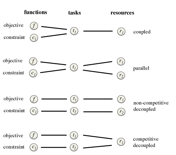
Figure 1: Schematic comparing the coupled, parallel, non-competitive decoupled (NCD), and competitive decoupled (CD) scenarios for a problem with a single constraint $c_{1}$. In each case, the mapping between tasks and resources (the right-hand portion of the figure) is the bipartite graph $\mathcal{G}$.

3.3 A General Algorithm for Constrained Bayesian Optimization

In this section we present a general algorithm for solving constrained Bayesian optimization problems specified according to the formalization from the previous section. Our approach relies on an acquisition function that can measure the expected utility of evaluating any arbitrary subset of functions, that is, of any possible task. When an acquisition function satisfies this requirement we say that it is separable. As discussed in Section 4.1, our method PESC has this property, when the functions are modeled as independent. This property makes PESC an effective solution for the practical implementation of our general algorithm. By contrast, the EIC-D method of Gelbart et al. (2014) is not separable and cannot be applied in the general case presented here.

Algorithm 1 provides a general procedure for solving constrained Bayesian optimization problems. The inputs to the algorithm are the set of functions $\mathcal{F}$, the set of tasks $\mathcal{T}$, the set of resources $\mathcal{R}$, the task-resource graph ${\mathcal{G}=(\mathcal{T}\cup\mathcal{R},\mathcal{E})}$, an acquisition function for each task, that is, $\alpha_{t}$ for $t\in\mathcal{T}$, the search space $\mathcal{X}$, a Bayesian model $\mathcal{M}$, the initial data set $\mathcal{D}$, the resource query functions $\omega$ and $\omega_{\text{max}}$ and a confidence level $\delta$ for making a final recommendation. Recall that $\omega_{\text{max}}$ indicates how many tasks can be simultaneously executed on a particular resource. The function $\omega$ is introduced here to indicate how many tasks are currently being evaluated in a resource. The acquisition function $\alpha_{t}$ measures the utility of evaluating task $t$ at the location $\mathbf{x}$. This acquisition function depends on the predictions of the Bayesian model $\mathcal{M}$. The separability property of the original acquisition function guarantees that we can compute an $\alpha_{t}$ for each $t\in\mathcal{T}$.

Algorithm 1 A general method for constrained Bayesian optimization.

1:  Input: $\mathcal{F}$, $\mathcal{G}=(\mathcal{T}\cup\mathcal{R},\mathcal{E})$, $\alpha_{t}$ for $t\in\mathcal{T}$, $\mathcal{X}$, $\mathcal{M}$, $\mathcal{D}$, $\omega$, $\omega_{\text{max}}$ and $\delta$.

2:  repeat

3:     for $r\in\mathcal{R}$ such that $\omega(r)<\omega_{\text{max}}(r)$ do

4:        Update $\mathcal{M}$ with any new data in $\mathcal{D}$

5:        for $t\in\mathcal{T}$ such that $\{t\sim r\}\in\mathcal{E}$ do

6:           $\mathbf{x}_{t}^{*}\leftarrow\arg\max_{\mathbf{x}\in\mathcal{X}}\alpha_{t}(\mathbf{x}|\mathcal{M})$

7:           $\alpha_{t}^{*}\leftarrow\alpha_{t}(\mathbf{x}_{t}^{*}|\mathcal{M})$

8:        end for

9:        $t^{*}\leftarrow\arg\max_{t}\,\alpha_{t}^{*}$

10:        Submit task $t^{*}$ at input $\mathbf{x}^{*}_{t^{*}}$ to resource $r$

11:        Update $\mathcal{M}$ with the new pending evaluation

12:     end for

13:  until termination condition is met

14:  Output: $\arg\min_{\mathbf{x}\in\mathcal{X}}\mathbb{E}_{\mathcal{M}}[f(\mathbf{x})]\;\,\mathrm{s.t.}\;p(c_{1}(\mathbf{x})\geq 0,\ldots,c_{K}(\mathbf{x})\geq 0|\mathcal{M})\geq 1-\delta$

Algorithm 1 works as follows. First, in line 3, we iterate over the resources, checking if they are available. Resource $r$ is available if its number of currently running jobs $\omega(r)$ is less than its capacity $\omega_{\text{max}}(r)$. Whenever resource $r$ is available, we check in line 4 if any new function observations have been collected. If this is the case, we then update the Bayesian model $\mathcal{M}$ with the new data (in most cases we will have new data since the resource $r$ probably became available due to the completion of a previous task). Next, we iterate in line 5 over the tasks $t$ that can be evaluated in the new available resource $r$ as dictated by $\mathcal{G}$. In line 6 we find the evaluation location $\mathbf{x}_{t}^{*}$ that maximizes the utility obtained by the evaluation of task $t$, as indicated by the task-specific acquisition function $\alpha_{t}$. In line 7 we obtain the corresponding maximum task utility $\alpha_{t}^{*}$. In line 9, we then maximize over tasks, selecting the task $t^{*}$ with highest maximum task utility $\alpha^{*}_{t}$ (this is the “competition” in CD). Upon doing so, the pair $(t^{*},\mathbf{x}^{*}_{t^{*}})$ forms the next suggestion. This pair represents the experiment with the highest acquisition function value over all possible $(t,\mathbf{x})$ pairs in $\mathcal{T}\times\mathcal{X}$ that can be run on resource $r$. In line 10, we evaluate the selected task at resource $r$ and in line 11 we update the Bayesian model $\mathcal{M}$ to take into account that we are expecting to collect data for task $t^{*}$ at input $\mathbf{x}^{*}_{t^{*}}$. This can be done for example by drawing virtual data from $\mathcal{M}$’s predictive distribution and then averaging across the predictions made when each virtual data point is assumed to be the data actually collected by the pending evaluation (Schonlau et al., 1998; Snoek et al., 2012). In line 13 the whole process repeats until a termination condition is met. Finally, in line 14, we give to the user a final recommendation of the solution to the optimization problem. This is the input that attains the lowest expected objective value subject to all the constraints being satisfied with posterior probability larger than $1-\delta$, where $\delta$ is maximum allowable probability of the recommendation being infeasible according to $\mathcal{M}$.

Algorithm 1 can solve problems that exhibit any combination of coupling, parallelism, NCD, and CD.

3.4 Incorporating Cost Information

Algorithm 1 always selects, among a group of competitive tasks, the one whose evaluation produces the highest utility value. However, other cost factors may render the evaluation of one task more desirable than another. The most salient of these costs is the run time or duration of the task’s evaluation, which could depend on the evaluation location $\mathbf{x}$. For example, in the neural network speech recognition system, one of the variables to be optimized may be the number of hidden units in the neural network. In this case, the run time of an evaluation of the predictive accuracy of the system is a function of $\mathbf{x}$ since the training time for the network scales with its size. Snoek et al. (2012) consider this issue by automatically measuring the duration of function evaluations. They model the duration as a function of $\mathbf{x}$ with an additional Gaussian process (GP). Swersky et al. (2013) extend this concept over multiple optimization tasks so that an independent GP is used to model the unknown duration of each task. This approach can be applied in Algorithm 1 by penalizing the acquisition function for task $t$ with the expected cost of evaluating that task. In particular, we can change lines 6 and 7 in Algorithm 1 to

• $\mathbf{x}_{t}^{*}\leftarrow\arg\max_{\mathbf{x}\in\mathcal{X}}\alpha_{t}(\mathbf{x}|\mathcal{M})/\zeta_{t}(\mathbf{x})$

• $\alpha_{t}^{*}\leftarrow\alpha_{t}(\mathbf{x}_{t}^{*}|\mathcal{M})/\zeta_{t}(\mathbf{x}_{t}^{*})$

where $\zeta_{t}(\mathbf{x})$ is the expected cost associated with the evaluation of task $t$ at $\mathbf{x}$, as estimated by a model of the collected cost data. When taking into account task costs modeled by Gaussian processes, the total number of GP models used by Algorithm 1 is equal to the number of functions in the constrained BO problem plus the number of tasks, that is, $|\mathcal{F}|+|\mathcal{T}|$. Alternatively, one could fix the cost functions $\zeta_{t}(\mathbf{x})$ a priori instead of learning them from collected data.

4 Predictive Entropy Search with Constraints (PESC)

To implement Algorithm 1 in practice we need to compute an acquisition function that is separable and can measure the utility of evaluating an arbitrary subset of functions. In this section we describe how to achieve this.

Our acquisition function approximates the expected gain of information about the solution to the constrained optimization problem, which is denoted by $\mathbf{x}_{\star}$. Importantly, our approximation is additive. For example, let $\mathcal{A}$ be a set of functions and let $I(\mathcal{A})$ be the amount of information that we approximately gain in expectation by jointly evaluating the functions in $\mathcal{A}$. Then $I(\mathcal{A})=\sum_{a\in\mathcal{A}}I(\{a\})$. Although our acquisition function is additive, the exact expected gain of information is not. Additivity is the result of a factorization assumption in our approximation (see Section 4.2 for further details). The good results obtained in our experiments seem to support that this is a reasonable assumption. Because of this additive property, we can compute an acquisition function for any possible subset of $f$, $c_{1},\ldots,c_{K}$ using the individual acquisition functions for these functions as building blocks.

We follow MacKay (1992) and measure information about $\mathbf{x}_{\star}$ by the differential entropy of $p(\mathbf{x}_{\star}|\mathcal{D})$, where $\mathcal{D}$ is the data collected so far. The distribution $p(\mathbf{x}_{\star}|\mathcal{D})$ is formally defined in the unconstrained case by Hennig and Schuler (2012). In the constrained case $p(\mathbf{x}_{\star}|\mathcal{D})$ can be understood as the probability distribution determined by the following sampling process. First, we draw $f$, $c_{1},\ldots,c_{K}$ from their posterior distributions given $\mathcal{D}$ and second, we minimize the sampled $f$ subject to the sampled $c_{1},\ldots,c_{K}$ being non-negative, that is, we solve Eq. 1 for the sampled functions. The solution to Eq. 1 obtained by this procedure represents then a sample from $p(\mathbf{x}_{\star}|\mathcal{D})$.

We consider first the case in which all the black-box functions $f,c_{1},\ldots,c_{K}$ are evaluated at the same time (coupled). Let $\text{H}\left[\mathbf{x}_{\star}\,|\,\mathcal{D}\right]$ denote the differential entropy of $p(\mathbf{x}_{\star}|\mathcal{D})$ and let $y_{f}$, $y_{c_{1}},\ldots,y_{c_{K}}$ denote the measurements obtained by querying the black-boxes for $f$, $c_{1},\ldots,c_{K}$ at the input location $\mathbf{x}$. We encode these measurements in vector form as ${\mathbf{y}=(y_{f},y_{c_{1}},\ldots,y_{c_{K}})^{\text{T}}}$. Note that $\mathbf{y}$ contains the result of the evaluation of all the functions at $\mathbf{x}$, that is, the objective $f$ and the constraints $c_{1},\ldots,c_{K}$. We aim to collect data at the location that maximizes the expected information gain or the expected reduction in the entropy of $p(\mathbf{x}_{\star}|\mathcal{D})$. The corresponding acquisition function is

$$\alpha(\mathbf{x})=\text{H}\left[\mathbf{x}_{\star}\,|\,\mathcal{D}\right]-\mathbb{E}_{\mathbf{y}\,|\,\mathcal{D},\mathbf{x}}\left[\text{H}\left[\mathbf{x}_{\star}\,|\,\mathcal{D}\cup\{(\mathbf{x},\mathbf{y})\}\right]\right]\,.$$ (7)

In this expression, $\text{H}\left[\mathbf{x}_{\star}\,|\,\mathcal{D}\cup\{(\mathbf{x},\mathbf{y})\}\right]$ is the amount of information on $\mathbf{x}_{\star}$ that is available once we have collected new data $\mathbf{y}$ at the input location $\mathbf{x}$. However, this new $\mathbf{y}$ is unknown because it has not been collected yet. To circumvent this problem, we take the expectation with respect to the predictive distribution for $\mathbf{y}$ given $\mathbf{x}$ and $\mathcal{D}$. This produces an expression that does not depend on $\mathbf{y}$ and could in principle be readily computed.

A direct computation of Eq. 7 is challenging because it requires evaluating the entropy of the intractable distribution $p(\mathbf{x}_{\star}\,|\,\mathcal{D})$ when different pairs $(\mathbf{x},\mathbf{y})$ are added to the data. To simplify computations, we note that Eq. 7 is the mutual information between $\mathbf{x}_{\star}$ and $\mathbf{y}$ given $\mathcal{D}$ and $\mathbf{x}$, which we denote by $\text{MI}(\mathbf{x}_{\star},\mathbf{y})$. The mutual information operator is symmetric, that is, $\text{MI}(\mathbf{x}_{\star},\mathbf{y})=\text{MI}(\mathbf{y},\mathbf{x}_{\star})$. Therefore, we can follow Houlsby et al. (2012) and swap the random variables $\mathbf{y}$ and $\mathbf{x}_{\star}$ in Eq. 7. The result is a reformulation of the original equation that is now expressed in terms of entropies of predictive distributions, which are easier to approximate:

$$\alpha(\mathbf{x})=\text{H}\left[\mathbf{y}\,|\,\mathcal{D},\mathbf{x}\right]-\mathbb{E}_{\mathbf{x}_{\star}\,|\,\mathcal{D}}\left[\text{H}\left[\mathbf{y}\,|\,\mathcal{D},\mathbf{x},\mathbf{x}_{\star}\right]\right]\,.$$ (8)

This is the same reformulation used by Predictive Entropy Search (PES) (Hernández-Lobato et al., 2014) for unconstrained Bayesian optimization, but extended to the case where $\mathbf{y}$ is a vector rather than a scalar. Since we focus on constrained optimization problems, we call our method Predictive Entropy Search with Constraints (PESC). Eq. 8 is used by PESC to efficiently solve constrained Bayesian optimization problems with decoupled function evaluations. In the following section we describe how to obtain a computationally efficient approximation to Eq. 8. We also show that the resulting approximation is separable.

4.1 The PESC Acquisition Function

We assume that the functions $f$, $c_{1},\ldots,c_{K}$ are independent samples from Gaussian process (GP) priors and that the noisy measurements $\mathbf{y}$ returned by the black-boxes are obtained by adding Gaussian noise to the noise-free function evaluations at $\mathbf{x}$. Under this Bayesian model for the data, the first term in Eq. 8 can be computed exactly. In particular,

$$\text{H}\left[\mathbf{y}\,|\,\mathcal{D},\mathbf{x}\right]=\sum_{i=1}^{K+1}\frac{1}{2}\log\sigma_{i}^{2}(\mathbf{x})+\frac{K+1}{2}\log(2\pi e)\,,$$ (9)

where $\sigma_{i}^{2}(\mathbf{x})$ is the predictive variance for $y_{i}$ at $\mathbf{x}$ and $y_{i}$ is the $i$-th entry in $\mathbf{y}$. To obtain this formula we have used the fact that $f$, $c_{1},\ldots,c_{K}$ are generated independently, so that $\text{H}\left[\mathbf{y}\,|\,\mathcal{D},\mathbf{x}\right]=\sum_{i=1}^{K+1}\text{H}\left[y_{i}\,|\,\mathcal{D},\mathbf{x}\right]$, and that $p(y_{i}\,|\,\mathcal{D},\mathbf{x})$ is Gaussian with variance parameter $\sigma_{i}^{2}(\mathbf{x})$ given by the GP predictive variance (Rasmussen and Williams, 2006):

$$\sigma_{i}^{2}(\mathbf{x})=k_{i}(\mathbf{x})-\mathbf{k}_{i}(\mathbf{x})^{\text{T}}\mathbf{K}^{-1}_{i}\mathbf{k}_{i}(\mathbf{x})+\nu_{i}\,,\quad\quad i=1,\ldots,K+1\,,$$ (10)

where $\nu_{i}$ is the variance of the additive Gaussian noise in the $i$-th black-box, with $f$ being the first one and $c_{K}$ the last one. The scalar $k_{i}(\mathbf{x})$ is the prior variance of the noise-free black-box evaluations at $\mathbf{x}$. The vector $\mathbf{k}_{i}(\mathbf{x})$ contains the prior covariances between the black-box values at $\mathbf{x}$ and at those locations for which data from the black-box is available. Finally, $\mathbf{K}_{i}$ is a matrix with the prior covariances for the noise-free black-box evaluations at those locations for which data is available.

The second term in Eq. 8, that is, $\mathbb{E}_{\mathbf{x}_{\star}\,|\,\mathcal{D}}\left[\text{H}\left[\mathbf{y}\,|\,\mathcal{D},\mathbf{x},\mathbf{x}_{\star}\right]\right]$, cannot be computed exactly and needs to be approximated. We do this operation as follows. : The expectation with respect to $p(\mathbf{x}_{\star}\,|\,\mathcal{D})$ is approximated with an empirical average over $M$ samples drawn from $p(\mathbf{x}_{\star}\,|\,\mathcal{D})$. These samples are generated by following the approach proposed by Hernández-Lobato et al. (2014) for sampling $\mathbf{x}_{\star}$ in the unconstrained case. We draw approximate posterior samples of $f,c_{1},\ldots,c_{K}$, as described by Hernández-Lobato et al. (2014, Appendix A), and then solve Eq. 1 to obtain $\mathbf{x}_{\star}$ given the sampled functions. More details can be found in Section B.3 of this document. Note that this approach only applies for stationary kernels, but this class includes popular choices such as the squared exponential and Matérn kernels. : We assume that the components of $\mathbf{y}$ are independent given $\mathcal{D}$, $\mathbf{x}$ and $\mathbf{x}_{\star}$, that is, we assume that the evaluations of $f$, $c_{1},\ldots,c_{K}$ at $\mathbf{x}$ are independent given $\mathcal{D}$ and $\mathbf{x}_{\star}$. This factorization assumption guarantees that the acquisition function used by PESC is additive across the different functions that are being evaluated. : Let $\mathbf{x}_{\star}^{j}$ be the $j$-th sample from $p(\mathbf{x}_{\star}\,|\,\mathcal{D})$. We then find a Gaussian approximation to each $p(y_{i}\,|\,\mathcal{D},\mathbf{x},\mathbf{x}_{\star}^{j})$ using expectation propagation (EP) (Minka, 2001a). Let $\sigma_{i}^{2}(\mathbf{x}|\mathbf{x}_{\star}^{j})$ be the variance of the Gaussian approximation to $p(y_{i}\,|\,\mathcal{D},\mathbf{x},\mathbf{x}_{\star}^{j})$ given by EP. Then, we obtain

$$\mathbb{E}_{\mathbf{x}_{\star}\,|\,\mathcal{D}}\left[\text{H}\left[\mathbf{y}\,|\,\mathcal{D},\mathbf{x},\mathbf{x}_{\star}\right]\right] \overset{\leavevmode\hbox to9.67pt{\vbox to9.67pt{\text{[drawing]}}}}{\approx}\frac{1}{M}\sum_{j=1}^{M}\text{H}\left[\mathbf{y}\,|\,\mathcal{D},\mathbf{x},\mathbf{x}_{\star}^{j}\right]\overset{\leavevmode\hbox to9.67pt{\vbox to9.67pt{\text{[drawing]}}}}{\approx}\frac{1}{M}\sum_{j=1}^{M}\left[\sum_{i=1}^{K+1}\text{H}\left[y_{i}\,|\,\mathcal{D},\mathbf{x},\mathbf{x}_{\star}^{j}\right]\right]$$

$$\overset{\leavevmode\hbox to9.67pt{\vbox to9.67pt{\text{[drawing]}}}}{\approx}\sum_{i=1}^{K+1}\left\{\frac{1}{M}\sum_{j=1}^{M}\frac{1}{2}\log\sigma_{i}^{2}(\mathbf{x}|\mathbf{x}_{\star}^{j})\right\}+\frac{K+1}{2}\log(2\pi e)\,,$$ (11)

where each of the approximations has been numbered with the corresponding step from the description above. Note that in step of Eq. 11 we have swapped the sums over $i$ and $j$.

The acquisition function used by PESC is then given by the difference between Eq. 9 and the approximation shown in the last line of Eq. 11. In particular, we obtain

$$\alpha_{\text{PESC}}(\mathbf{x})=\sum_{i=1}^{K+1}\tilde{\alpha}_{i}(\mathbf{x})\,,$$ (12)

where

$$\tilde{\alpha}_{i}(\mathbf{x})=\frac{1}{M}\sum_{j=1}^{M}\underbrace{\frac{1}{2}\log\sigma_{i}^{2}(\mathbf{x})-\frac{1}{2}\log\sigma_{i}^{2}(\mathbf{x}|\mathbf{x}_{\star}^{j})}_{\textstyle\tilde{\alpha}_{i}(\mathbf{x}|\mathbf{x}_{\star}^{j})}\,,\quad\quad i=1,\ldots,K+1\,.$$ (13)

Interestingly, the factorization assumption that we made in step of Eq. 11 has produced an acquisition function in Eq. 12 that is the sum of $K+1$ function-specific acquisition functions, given by the $\tilde{\alpha}_{i}(\mathbf{x})$ in Eq. 13. Each $\tilde{\alpha}_{i}(\mathbf{x})$ measures how much information we gain on average by only evaluating the $i$-th black box, where the first black-box evaluates $f$ and the last one evaluates $c_{K+1}$. Furthermore, $\tilde{\alpha}_{i}(\mathbf{x})$ is the empirical average of $\tilde{\alpha}_{i}(\mathbf{x}|\mathbf{x}_{\star})$ across $M$ samples from $p(\mathbf{x}_{\star}|\mathcal{D})$. Therefore, we can interpret each $\tilde{\alpha}_{i}(\mathbf{x}|\mathbf{x}_{\star})$ in Eq. 13 as a function-specific acquisition function conditioned on $\mathbf{x}_{\star}$. Crucially, by using bits of information about the minimizer as a common unit of measurement, our acquisition function can make meaningful comparisons between the usefulness of evaluating the objective and constraints.

We now show how PESC can be used to obtain the task-specific acquisition functions required by the general algorithm from Section 3.3. Let us assume that we plan to evaluate only a subset of the functions $f$, $c_{1},\ldots,c_{K}$ and let $t\subseteq\{1,\ldots,K+1\}$ contain the indices of the functions to be evaluated, where the first function is $f$ and the last one is $c_{K}$. We assume that the functions indexed by $t$ are coupled and require joint evaluation. In this case $t$ encodes a task according to the definition from Section 3.2. We can then approximate the expected gain of information that is obtained by evaluating this task at input $\mathbf{x}$. The process is similar to the one used above when all the black-boxes are evaluated at the same time. However, instead of working with the full vector $\mathbf{y}$, we now work with the components of $\mathbf{y}$ indexed by $t$. One can then show that the expected information gain obtained after evaluating task $t$ at input $\mathbf{x}$ can be approximated as

$$\alpha_{t}(\mathbf{x})=\sum_{i\in t}\tilde{\alpha}_{i}(\mathbf{x})\,,$$ (14)

where the $\tilde{\alpha}_{i}$ are given by Eq. 13. PESC’s acquisition function is therefore separable since Eq. 14 can be used to obtain an acquisition function for each possible task. The process for constructing these task-specific acquisition functions is also efficient since it requires only to use the individual acquisition functions from Eq. 13 as building blocks. These two properties make PESC an effective solution for the practical implementation of the general algorithm from Section 3.3.

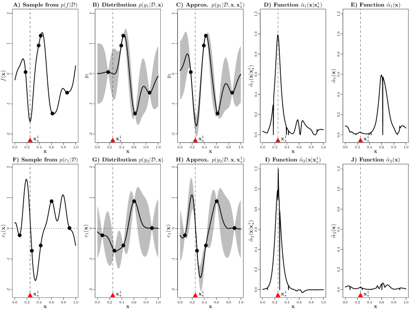
Figure 2: Illustration of the process followed to compute the function-specific acquisition functions given by Eq. 13. See the main text for details.

Fig. 2 illustrates with a toy example the process for computing the function-specific acquisition functions from Eq. 13. In this example there is only one constraint function. Therefore, the functions in the optimization problem are only $f$ and $c_{1}$. The search space $\mathcal{X}$ is the unit interval $[0,1]$ and we have collected four measurements for each function. The data for $f$ are shown as black points in panels A, B and C. The data for $c_{1}$ are shown as black points in panels F, G and H. We assume that $f$ and $c_{1}$ are independently sampled from a GP with zero mean function and squared exponential covariance function with unit amplitude and length-scale $0.07$. The noise variance for the black-boxes that evaluate $f$ and $c_{1}$ is zero. Let $y_{1}$ and $y_{2}$ be the black-box evaluations for $f$ and $c_{1}$ at input $\mathbf{x}$. Under the assumed GP model we can analytically compute the predictive distributions for $y_{1}$ and $y_{2}$, that is, $p(y_{1}|\mathcal{D},\mathbf{x})$ and $p(y_{2}|\mathcal{D},\mathbf{x})$. Panels B and G show the means of these distributions with confidence bands equal to one standard deviation. The first step to compute the $\tilde{\alpha}_{i}(\mathbf{x})$ from Eq. 13 is to draw $M$ samples from $p(\mathbf{x}_{\star}|\mathcal{D})$. To generate each of these samples, we first approximately sample $f$ and $c_{1}$ from their posterior distributions $p(f|\mathcal{D})$ and $p(c_{1}|\mathcal{D})$ using the method described by Hernández-Lobato et al. (2014, Appendix A). Panels A and F show one of the samples obtained for $f$ and $c_{1}$, respectively. We then solve the optimization problem given by Eq. 1 when $f$ and $c_{1}$ are known and equal to the samples obtained. The solution to this problem is the input that minimizes $f$ subject to $c_{1}$ being positive. This produces a sample $\mathbf{x}_{\star}^{1}$ from $p(\mathbf{x}_{\star}|\mathcal{D})$ which is shown as a discontinuous vertical line with a red triangle in all the panels. The next step is to find a Gaussian approximation to the predictive distributions when we condition to $\mathbf{x}_{\star}^{1}$, that is, $p(y_{1}|\mathcal{D},\mathbf{x},\mathbf{x}_{\star}^{1})$ and $p(y_{2}|\mathcal{D},\mathbf{x},\mathbf{x}_{\star}^{1})$. This step is performed using expectation propagation (EP) as described in Section 4.2 and Appendix A. Panels C and H show the approximations produced by EP for $p(y_{1}|\mathcal{D},\mathbf{x},\mathbf{x}_{\star}^{1})$ and $p(y_{2}|\mathcal{D},\mathbf{x},\mathbf{x}_{\star}^{1})$, respectively. Panel C shows that conditioning to $\mathbf{x}_{\star}^{1}$ decreases the posterior mean of $y_{1}$ in the neighborhood of $\mathbf{x}_{\star}^{1}$. The reason for this is that $\mathbf{x}_{\star}^{1}$ must be the global feasible solution and this means that $f(\mathbf{x}_{\star}^{1})$ must be lower than any other feasible point. Panel H shows that conditioning to $\mathbf{x}_{\star}^{1}$ increases the posterior mean of $y_{2}$ in the neighborhood of $\mathbf{x}_{\star}^{1}$. The reason for this is that $c_{1}(\mathbf{x}_{\star}^{1})$ must be positive because $\mathbf{x}_{\star}^{1}$ has to be feasible. In particular, by conditioning to $\mathbf{x}_{\star}^{1}$ we are giving zero probability to all $c_{1}$ such that $c_{1}(\mathbf{x}_{\star}^{1})<0$. Let $\sigma_{1}^{2}(\mathbf{x}|\mathbf{x}_{\star}^{1})$ and $\sigma_{2}^{2}(\mathbf{x}|\mathbf{x}_{\star}^{1})$ be the variances of the Gaussian approximations to $p(y_{1}|\mathcal{D},\mathbf{x},\mathbf{x}_{\star}^{1})$ and $p(y_{2}|\mathcal{D},\mathbf{x},\mathbf{x}_{\star}^{1})$ and let $\sigma_{1}^{2}(\mathbf{x})$ and $\sigma_{2}^{2}(\mathbf{x})$ be the variances of $p(y_{1}|\mathcal{D},\mathbf{x})$ and $p(y_{2}|\mathcal{D},\mathbf{x})$. We use these quantities to obtain $\tilde{\alpha}_{1}(\mathbf{x}|\mathbf{x}_{\star}^{1})$ and $\tilde{\alpha}_{2}(\mathbf{x}|\mathbf{x}_{\star}^{1})$ according to Eq. 13. These two functions are shown in panels D and I. The whole process is repeated $M=50$ times and the resulting $\tilde{\alpha}_{1}(\mathbf{x}|\mathbf{x}_{\star}^{j})$ and $\tilde{\alpha}_{2}(\mathbf{x}|\mathbf{x}_{\star}^{j})$, $j=1,\ldots,M$, are averaged according to Eq. 13 to obtain the function-specific acquisition functions $\tilde{\alpha}_{1}(\mathbf{x})$ and $\tilde{\alpha}_{2}(\mathbf{x})$, whose plots are shown in panels E and J. These plots indicate that evaluating the objective $f$ is in this case more informative than evaluating the constraint $c_{1}$. But this is certainly not always the case, as will be demonstrated in the experiments later on.

4.2 How to Compute the Gaussian Approximation to $p(y_{i}|\mathcal{D},\mathbf{x},\mathbf{x}_{\star}^{j})$

We briefly describe the process followed to find a Gaussian approximation to $p(y_{i}|\mathcal{D},\mathbf{x},\mathbf{x}_{\star}^{j})$ using expectation propagation (EP) (Minka, 2001b). Recall that the variance of this approximation, that is, $\sigma_{i}^{2}(\mathbf{x}|\mathbf{x}_{\star}^{j})$, is used to compute $\tilde{\alpha}_{i}(\mathbf{x}|\mathbf{x}_{\star}^{j})$ in Eq. 13. Here we only provide a sketch of the process; full details can be found in Appendix A.

We start by assuming that the search space has finite size, that is, $\mathcal{X}=\{\tilde{\mathbf{x}}_{1},\ldots,\tilde{\mathbf{x}}_{|\mathcal{X}|}\}$. In this case the functions $f$, $c_{1},\ldots,c_{K}$ are encoded as finite dimensional vectors denoted by $\mathbf{f}$, $\mathbf{c}_{1},\ldots,\mathbf{c}_{K}$. The $i$-th entries in these vectors are the result of evaluating $f$, $c_{1},\ldots,c_{K}$ at the $i$-th element of $\mathcal{X}$, that is, $f(\tilde{\mathbf{x}})$, $c_{1}(\tilde{\mathbf{x}}_{i}),\ldots,c_{K}(\tilde{\mathbf{x}}_{i})$. Let us assume that $\mathbf{x}_{\star}^{j}$ and $\mathbf{x}$ are in $\mathcal{X}$. Then $p(\mathbf{y}|\mathcal{D},\mathbf{x},\mathbf{x}_{\star}^{j})$ can be defined by the following rejection sampling process. First, we sample $\mathbf{f}$, $\mathbf{c}_{1},\ldots,\mathbf{c}_{K}$ from their posterior distribution given the assumed GP models. We then solve the optimization problem given by Eq. 1. For this, we find the entry of $\mathbf{f}$ with lowest value subject to the corresponding entries of $\mathbf{c}_{1},\ldots,\mathbf{c}_{K}$ being positive. Let $i\in\{1,\ldots,|\mathcal{X}|\}$ be the index of the selected entry. Then, if $\mathbf{x}_{\star}^{j}\neq\tilde{\mathbf{x}}_{i}$, we reject the sampled $\mathbf{f}$, $\mathbf{c}_{1},\ldots,\mathbf{c}_{K}$ and start again. Otherwise, we take the entries of $\mathbf{f}$, $\mathbf{c}_{1},\ldots,\mathbf{c}_{K}$ indexed by $\mathbf{x}$, that is, $f(\mathbf{x})$, $c_{1}(\mathbf{x}),\ldots,c_{K}(\mathbf{x})$ and then obtain $\mathbf{y}$ by adding to each of these values a Gaussian random variable with zero mean and variance $\nu_{1},\ldots,\nu_{K+1}$, respectively. The probability distribution implied by this rejection sampling process can be obtained by first multiplying the posterior for $\mathbf{f}$, $\mathbf{c}_{1},\ldots,\mathbf{c}_{K}$ with indicator functions that take value zero when $\mathbf{f}$, $\mathbf{c}_{1},\ldots,\mathbf{c}_{K}$ should be rejected and one otherwise. We can then multiply the resulting quantity by the likelihood for $\mathbf{y}$ given $\mathbf{f}$, $\mathbf{c}_{1},\ldots,\mathbf{c}_{K}$. The desired distribution is finally obtained by marginalizing out $\mathbf{f}$, $\mathbf{c}_{1},\ldots,\mathbf{c}_{K}$.

We introduce several indicator functions to implement the approach described above. The first one $\Gamma(\mathbf{x})$ takes value one when $\mathbf{x}$ is a feasible solution and value zero otherwise, that is,

$$\Gamma(\mathbf{x})=\prod_{k=1}^{K}\Theta[c_{k}(\mathbf{x})]\,,$$ (15)

where $\Theta[\cdot]$ is the Heaviside step function which is equal to one if its input is non-negative and zero otherwise. The second indicator function $\Psi(\mathbf{x})$ takes value zero if $\mathbf{x}$ is a better solution than $\mathbf{x}_{\star}^{j}$ according to the sampled functions. Otherwise $\Psi(\mathbf{x})$ takes value one. In particular,

$$\Psi(\mathbf{x})=\Gamma(\mathbf{x})\Theta[f(\mathbf{x})-f(\mathbf{x}_{\star}^{j})]+\left(1-\Gamma(\mathbf{x})\right)\,.$$ (16)

When $\mathbf{x}$ is infeasible, this expression takes value one. In this case, $\mathbf{x}$ is not a better solution than $\mathbf{x}_{\star}^{j}$ (because $\mathbf{x}$ is infeasible) and we do not have to reject. When $\mathbf{x}$ is feasible, the factor $\Theta[f(\mathbf{x})-f(\mathbf{x}_{\star}^{j})]$ in Eq. 16 is zero when $\mathbf{x}$ takes lower objective value than $\mathbf{x}_{\star}^{j}$. This will allow us to reject $\mathbf{f}$, $\mathbf{c}_{1},\ldots,\mathbf{c}_{K}$ when $\mathbf{x}$ is a better solution than $\mathbf{x}_{\star}^{j}$. Using Eq. 15 and Eq. 16, we can then write $p(\mathbf{y}|\mathcal{D},\mathbf{x},\mathbf{x}_{\star}^{j})$ as

$$\leavevmode\resizebox{422.77661pt}{}{$p(\mathbf{y}|\mathcal{D},\mathbf{x},\mathbf{x}_{\star}^{j})\propto\int p(\mathbf{y}|\mathbf{f},\mathbf{c}_{1},\ldots,\mathbf{c}_{K},\mathbf{x})\underbrace{p(\mathbf{f},\mathbf{c}_{1},\ldots,\mathbf{c}_{K}|\mathcal{D})\Gamma(\mathbf{x}_{\star}^{j})\left\{\prod_{\mathbf{x}^{\prime}\in\mathcal{X}}\Psi(\mathbf{x}^{\prime})\right\}}_{\textstyle f(\mathbf{f},\mathbf{c}_{1},\ldots,\mathbf{c}_{K}|\mathbf{x}_{\star}^{j})}\,d\mathbf{f}\,d\mathbf{c}_{1}\cdots\mathbf{c}_{K}$}\,,$$ (17)

where $p(\mathbf{f},\mathbf{c}_{1},\ldots,\mathbf{c}_{K}|\mathcal{D})$ is the GP posterior distribution for the noise-free evaluations of $f$, $c_{1},\ldots,c_{K}$ at $\mathcal{X}$ and $p(\mathbf{y}|\mathbf{f},\mathbf{c}_{1},\ldots,\mathbf{c}_{K},\mathbf{x})$ is the likelihood function, that is, the distribution of the noisy evaluations produced by the black-boxes with input $\mathbf{x}$ given the true function values:

$$\leavevmode\resizebox{422.77661pt}{}{$p(\mathbf{y}|\mathbf{f},\mathbf{c}_{1},\ldots,\mathbf{c}_{K},\mathbf{x})=\mathcal{N}(y_{1}|f(\mathbf{x}),\nu_{1})\mathcal{N}(y_{2}|c_{1}(\mathbf{x}),\nu_{2})\cdots\mathcal{N}(y_{K+1}|c_{K}(\mathbf{x}),\nu_{K+1})$}\,.$$ (18)

The product of the indicator functions $\Gamma$ and $\Psi$ in Eq. 17 takes value zero whenever $\mathbf{x}_{\star}^{j}$ is not the best feasible solution according to $\mathbf{f},\mathbf{c}_{1},\ldots,\mathbf{c}_{K}$. The indicator $\Gamma$ in Eq. 17 guarantees that $\mathbf{x}_{\star}^{j}$ is a feasible location. The product of all the $\Psi$ in Eq. 17 guarantees that no other point in $\mathcal{X}$ is better than $\mathbf{x}_{\star}^{j}$. Therefore, the product of $\Gamma$ and the $\Psi$ in Eq. 17 rejects any value of $\mathbf{f},\mathbf{c}_{1},\ldots,\mathbf{c}_{K}$ for which $\mathbf{x}_{\star}^{j}$ is not the optimal solution to the constrained optimization problem.

The factors $p(\mathbf{f},\mathbf{c}_{1},\ldots,\mathbf{c}_{K}|\mathcal{D})$ and $p(\mathbf{y}|\mathbf{f},\mathbf{c}_{1},\ldots,\mathbf{c}_{K},\mathbf{x})$ in Eq. 17 are Gaussian. Thus, their product is also Gaussian and tractable. However, the integral in Eq. 17 does not have a closed form solution because of the complexity introduced by the the product of indicator functions $\Gamma$ and $\Psi$. This means that Eq. 17 cannot be exactly computed and has to be approximated. For this, we use EP to fit a Gaussian approximation to the product of $p(\mathbf{f},\mathbf{c}_{1},\ldots,\mathbf{c}_{K}|\mathcal{D})$ and the indicator functions $\Gamma$ and $\Psi$ in Eq. 17, which we have denoted by $f(\mathbf{f},\mathbf{c}_{1},\ldots,\mathbf{c}_{K}|\mathbf{x}_{\star}^{j})$, with a tractable Gaussian distribution given by

$$q(\mathbf{f},\mathbf{c}_{1},\ldots,\mathbf{c}_{K}|\mathbf{x}_{\star}^{j})=\mathcal{N}(\mathbf{f}|\mathbf{m}_{1},\mathbf{V}_{1})\mathcal{N}(\mathbf{c}_{1}|\mathbf{m}_{2},\mathbf{V}_{2})\cdots\mathcal{N}(\mathbf{c}_{K}|\mathbf{m}_{K+1},\mathbf{V}_{K+1})\,,$$ (19)

where $\mathbf{m}_{1},\ldots,\mathbf{m}_{K+1}$ and $\mathbf{V}_{1},\ldots,\mathbf{V}_{K+1}$ are mean vectors and covariance matrices to be determined by the execution of EP. Let $v_{i}(\mathbf{x})$ be the diagonal entry of $\mathbf{V}_{i}$ corresponding to the evaluation location given by $\mathbf{x}$, where $i=1,\ldots,K+1$. Similarly, let $m_{i}(\mathbf{x})$ be the entry of $\mathbf{m}_{i}$ corresponding to the evaluation location $\mathbf{x}$ for $i=1,\ldots,K+1$. Then, by replacing $f(\mathbf{f},\mathbf{c}_{1},\ldots,\mathbf{c}_{K}|\mathbf{x}_{\star}^{j})$ in Eq. 17 with $q(\mathbf{f},\mathbf{c}_{1},\ldots,\mathbf{c}_{K}|\mathbf{x}_{\star}^{j})$, we obtain

$$p(\mathbf{y}|\mathcal{D},\mathbf{x},\mathbf{x}_{\star}^{j})\approx\prod_{i=1}^{K+1}\mathcal{N}(y_{i}|m_{i}(\mathbf{x}),v_{i}(\mathbf{x})+\nu_{i})\,.$$ (20)

Consequently, $\sigma_{i}^{2}(\mathbf{x}|\mathbf{x}_{\star}^{j})=v_{i}(\mathbf{x})+\nu_{i}$ can be used to compute $\tilde{\alpha}_{i}(\mathbf{x}|\mathbf{x}_{\star}^{j})$ in Eq. 13.

The previous approach does not work when the search space $\mathcal{X}$ has infinite size, for example when $\mathcal{X}=[0,1]^{d}$ with $d$ being the dimension of the inputs to $f,c_{1},\ldots,c_{K}$. In this case the product of indicators in Eq. 17 includes an infinite number of factors $\Psi(\mathbf{x}^{\prime})$, one for each possible $\mathbf{x}^{\prime}\in\mathcal{X}$. To solve this problem we perform an additional approximation. For the computation of Eq. 17, we consider that $\mathcal{X}$ is well approximated by the finite set $\mathcal{Z}$, which contains only the locations at which the objective $f$ has been evaluated so far, the value of $\mathbf{x}_{\star}^{j}$ and $\mathbf{x}$. Therefore, we approximate the factor $\prod_{\mathbf{x}^{\prime}\in\mathcal{X}}\Psi(\mathbf{x}^{\prime})$ in Eq. 17 with the factor $\prod_{\mathbf{x}^{\prime}\in\mathcal{Z}}\Psi(\mathbf{x}^{\prime})$, which has now finite size. We expect this approximation to become more and more accurate as we increase the amount of data collected for $f$. Note that our approximation to $\mathcal{X}$ is finite, but it is also different for each location $\mathbf{x}$ at which we want to evaluate Eq. 17 since $\mathcal{Z}$ is defined to contain $\mathbf{x}$. A detailed description of the resulting EP algorithm, indicating how to compute the variance functions $v_{i}(\mathbf{x})$ shown in Eq. 20, is given in Appendix A.

The EP approximation to Eq. 20, performed after replacing $\mathcal{X}$ with $\mathcal{Z}$, depends on the values of $\mathcal{D}$, $\mathbf{x}_{\star}^{j}$ and $\mathbf{x}$. Having to re-run EP for each value of $\mathbf{x}$ at which we may want to evaluate the acquisition function given by Eq. 12 is a very expensive operation. To avoid this, we split the EP computations between those that depend only on $\mathcal{D}$ and $\mathbf{x}_{\star}^{j}$, which are the most expensive ones, and those that depend only on the value of $\mathbf{x}$. We perform the former computations only once and then reuse them for each different value of $\mathbf{x}$. This allows us to evaluate the EP approximation to Eq. 17 at different values of $\mathbf{x}$ in a computationally efficient way. See Appendix A for further details.

4.3 Efficient Marginalization of the Model Hyper-parameters

So far we have assumed to know the optimal hyper-parameter values, that is, the amplitude and the length-scales for the GPs and the noise variances for the black-boxes. However, in practice, the hyper-parameter values are unknown and have to be estimated from data. This can be done for example by drawing samples from the posterior distribution of the hyper-parameters under some non-informative prior. Ideally, we should then average the GP predictive distributions with respect to the generated samples before approximating the information gain. However, this approach is too computationally expensive in practice. Instead, we follow Snoek et al. (2012) and average the PESC acquisition function with respect to the generated hyper-parameter samples. In our case, this involves marginalizing each of the function-specific acquisition functions from Eq. 13. For this, we follow the method proposed by Hernández-Lobato et al. (2014) to average the acquisition function of Predictive Entropy Search in the unconstrained case. Let $\bm{\Theta}$ denote the model hyper-parameters. First, we draw $M$ samples $\bm{\Theta}^{1},\ldots,\bm{\Theta}^{M}$ from the posterior distribution of $\bm{\Theta}$ given the data $\mathcal{D}$. Typically, for each of the posterior samples $\bm{\Theta}^{j}$ of $\bf\Theta$ we draw a single corresponding sample $\mathbf{x}_{\star}^{j}$ from the posterior distribution of $\mathbf{x}_{\star}$ given $\bm{\Theta}^{j}$, that is, $p(\mathbf{x}_{\star}\,|\,\mathcal{D},\bm{\Theta}^{j})$. Let $\sigma_{i}^{2}(\mathbf{x}|\bm{\Theta}^{j})$ be the variance of the GP predictive distribution for $y_{i}$ when the hyper-parameter values are fixed to $\bm{\Theta}^{j}$, that is, $p(y_{i}|\mathcal{D},\mathbf{x},\bm{\Theta}^{j})$, and let $\sigma_{i}^{2}(\mathbf{x}|\mathbf{x}_{\star}^{j},\bm{\Theta}^{j})$ be the variance of the Gaussian approximation to the predictive distribution for $y_{i}$ when we condition to the solution of the optimization problem being $\mathbf{x}_{\star}^{j}$ and the hyper-parameter values being $\bm{\Theta}^{j}$. Then, the version of Eq. 13 that marginalizes out the model hyper-parameters is given by

$$\tilde{\alpha}_{i}(\mathbf{x})=\frac{1}{M}\sum_{j=1}^{M}\left\{\frac{1}{2}\log\sigma_{i}^{2}(\mathbf{x}|\bm{\Theta}^{j})-\frac{1}{2}\log\sigma_{i}^{2}(\mathbf{x}|\mathbf{x}_{\star}^{j},\bm{\Theta}^{j})\right\}\,,\quad\quad i=1,\ldots,K+1\,.$$ (21)

Note that $j$ is now an index over joint posterior samples of the model hyper-parameters $\bm{\Theta}$ and the constrained minimizer $\mathbf{x}_{\star}$. Therefore, we can marginalize out the hyper-parameter values without adding any additional computational complexity to our method because a loop over $M$ samples of $\mathbf{x}_{\star}$ is just replaced with a loop over $M$ joint samples of $(\Theta,\mathbf{x}_{\star})$. This is a consequence of our reformulation of Eq. 7 into Eq. 8. By contrast, other techniques that work by approximating the original form of the acquisition function used in Eq. 7 do not have this property. An example in the unconstrained setting is Entropy Search (Hennig and Schuler, 2012), which requires re-computing an approximation to the acquisition function for each hyper-parameter sample $\bm{\Theta}^{j}$.

4.4 Computational Complexity

In the coupled setting, the complexity of PESC is $\mathcal{O}(MKN^{3})$, where $M$ is the number of posterior samples of the global constrained minimizer $\mathbf{x}_{\star}$, $K$ is the number of constraints, and $N$ is the number of collected data points. This cost is determined by the cost of each EP iteration, which requires computing the inverse of the covariance matrices $\mathbf{V}_{1},\ldots,\mathbf{V}_{K+1}$ in Eq. 20. The dimensionality of each of these matrices grows with the size of $\mathcal{Z}$, which is determined by the number $N$ of objective evaluations (see the last paragraph of Section 4.2). Therefore each EP iteration has cost $\mathcal{O}(KN^{3})$ and we have to run an instance of EP for each of the $M$ samples of $\mathbf{x}_{\star}$. If $M$ is also the number of posterior samples for the GP hyperparameters, as explained in Section 4.3, this is the same computational complexity as in EIC. However, in practice PESC is slower than EIC because of the cost of running multiple iterations of the EP algorithm.

In the decoupled setting the cost of PESC is ${\mathcal{O}(M\sum_{k=2}^{K+1}(N_{1}+N_{k})^{3})}$ where $N_{1}$ is the number of evaluations of the objective and $N_{k}$ is the number of evaluations for constraint $k-1$. The origin of this cost is again the size of the matrices $\mathbf{V}_{1},\ldots,\mathbf{V}_{K+1}$ in Eq. 20. While $\mathbf{V}_{1}$ still scales as a function of $|\mathcal{Z}|$, we have that $\mathbf{V}_{2},\ldots,\mathbf{V}_{K+1}$ scale now as a function of $|\mathcal{Z}|$ plus the number of observations for the corresponding constraint function. The reason for this is that $\prod_{\mathbf{x}^{\prime}\in\mathcal{Z}}\Psi(\mathbf{x}^{\prime})$ is used to approximate $\prod_{\mathbf{x}^{\prime}\in\mathcal{X}}\Psi(\mathbf{x}^{\prime})$ in Eq. 17 and each factor in $\prod_{\mathbf{x}^{\prime}\in\mathcal{Z}}\Psi(\mathbf{x}^{\prime})$ represents then a virtual data point for each GP. See Appendix A for details.

The cost of sampling the GP hyper-parameters is $\mathcal{O}(MKN^{3})$ and therefore, it does not affect the overall computational complexity of PESC.

4.5 Relationship between PESC and PES

PESC can be applied to unconstrained optimization problems. For this we only have to set $K=0$ and ignore the constraints. The resulting technique is very similar to the method PES proposed by Hernández-Lobato et al. (2014) as an information-based approach for unconstrained Bayesian optimization. However, PESC without constraints and PES are not identical. PES approximates $p(y|\mathcal{D},\mathbf{x},\mathbf{x}_{\star}^{j})$ by multiplying the GP predictive distribution by additional factors that enforce $\mathbf{x}_{\star}^{j}$ to be the location with lowest objective value. These factors guarantee that 1) the value of the objective at $\mathbf{x}_{\star}^{j}$ is lower than the minimum of the values for the objective collected so far, 2) the gradient of the objective is zero at $\mathbf{x}_{\star}$ and 3) the Hessian of the objective is positive definite at $\mathbf{x}_{\star}$. We do not enforce the last two conditions since the global optimum may be on the boundary of a feasible region and thus conditions 2) and 3) do not necessarily hold (this issue also arises in PES because the optimum may be on the boundary of the search space $\mathcal{X}$). Condition 1) is implemented in PES by taking the minimum observed value for the objective, denoted by $\eta$, and then imposing the soft condition $f(\mathbf{x}_{\star}^{j})<\eta+\epsilon$, where $\epsilon\sim\mathcal{N}(0,\nu)$ accounts for the additive Gaussian noise with variance $\nu$ in the black-box that evaluates the objective. In PESC this is achieved in a more principled way by using the indicator functions given by Eq. 16.

4.6 Summary of the Approximations Made in PESC

We describe here all the approximations performed in the practical implementation of PESC. PESC approximates the expected reduction in the posterior entropy of $\mathbf{x}_{\star}$ (see Eq. 7) with the acquisition function given by Eq. 12. This involves the following approximations:

1. The expectation over $\mathbf{x}_{\star}$ in Eq. 8 is approximated with Monte Carlo sampling.

2. The Monte Carlo samples of $\mathbf{x}_{\star}$ come from samples of $f,c_{1},\ldots,c_{K}$ drawn approximately using a finite basis function approximation to the GP covariance function, as described by Hernández-Lobato et al. (2014, Appendix A).

3. We approximate the factor $\prod_{\mathbf{x}^{\prime}\in\mathcal{X}}\Psi(\mathbf{x}^{\prime})$ in Eq. 17 with the factor $\prod_{\mathbf{x}^{\prime}\in\mathcal{Z}}\Psi(\mathbf{x}^{\prime})$. Unlike the original search space $\mathcal{X}$, $\mathcal{Z}$ has now finite size and the corresponding product of $\Psi$ indicators is easier to approximate. The set $\mathcal{Z}$ is formed by the locations of the current observations for the objective $f$ and the current evaluation location $\mathbf{x}$ of the acquisition function.

4. After replacing $\prod_{\mathbf{x}^{\prime}\in\mathcal{X}}\Psi(\mathbf{x}^{\prime})$ with $\prod_{\mathbf{x}^{\prime}\in\mathcal{Z}}\Psi(\mathbf{x}^{\prime})$ in Eq. 17, we further approximate the factor $f(\mathbf{f},\mathbf{c}_{1},\ldots,\mathbf{c}_{K}|\mathbf{x}_{\star}^{j})$ in this equation with the Gaussian approximation given by the right-hand-side of Eq. 20. We use the method expectation propagation (EP) for this task, as described in Appendix A. Because the EP approximation in Eq. 19 factorizes across $\mathbf{f}$, $\mathbf{c}_{1},\ldots,\mathbf{c}_{K}$, the execution of EP implicitly includes the factorization assumption performed in step of Eq. 11.

5. As described in the last paragraph of Section 4.2, in the execution of EP we separate the computations that depend on $\mathcal{D}$ and $\mathbf{x}_{\star}^{j}$, which are very expensive, from those that depend on the location $\mathbf{x}$ at which the PESC acquisition function will be evaluated. This allows us to evaluate the approximation to Eq. 17 at different values of $\mathbf{x}$ in a computationally efficient way.

6. To deal with unknown hyper-parameter values, we marginalize the acquisition function over posterior samples of the hyper-parameters. Ideally, we should instead marginalize the predictive distributions with respect to the hyper-parameters before computing the entropy, but this is too computationally expensive in practice.

In Section 6.1, we assess the accuracy of these approximations (except the last one) and show that PESC performs on par with a ground-truth method based on rejection sampling.

Note that in addition to the mathematical approximations described above, additional sources of error are introduced by the numerical computations involved. In addition to the usual roundoff error, etc., we draw the reader’s attention to the fact that the $\mathbf{x}_{\star}$ samples are the result of numerical global optimization of the approximately drawn samples of $f,c_{1},\ldots,c_{K}$, and then the suggestion is chosen by another numerical global optimization of the acquisition function. At present, we do not have guarantees that the true global optimum is found by our numerical methods in each case.

5 PESC-F: Speeding Up the BO Computations

One disadvantage of PESC is that sampling $\mathbf{x}_{\star}$ and then computing the corresponding EP approximation can be slow. If PESC is slow with respect to the evaluation of the black-box functions $f,c_{1},\ldots,c_{K}$, the entire Bayesian optimization (BO) procedure may be inefficient. For the BO approach to be useful, the time spent doing meta-computations has to be significantly shorter than the time spent actually evaluating the objective and constraints. This issue can be avoided in the coupled case by, for example, switching to a faster acquisition function like EIC or abandoning BO entirely for methods such as the popular CMA-ES (Hansen and Ostermeier, 1996) evolutionary strategy. However, in the decoupling setting, one can encounter problems in which some tasks are fast and others are slow. In this case, a cumbersome BO method might be undesirable because it would be unreasonable to spend minutes making a decision about a task that only takes seconds to complete; and, yet, a method that is fast but inefficient in terms of function evaluations would be ill-suited to making decisions about a task that takes hours complete. This situation calls for an optimization algorithm that can adaptively adjust its own decision-making time. For this reason, we introduce additional approximations in the computations made by PESC to reduce their cost when necessary. The new method that adaptively switches between fast and slow decision-making computations is called PESC-F. The two main challenges are how to speed up the original computations made by PESC and how to decide when to switch between the slow and the fast versions of those computations. In the following paragraphs we address these issues.

We propose ways to reduce the cost of the computations performed by PESC after collecting each new data point. These computations include

1. Drawing posterior samples of the GP hyper-parameters and then for each sample computing the Cholesky decomposition of the kernel matrix.

2. Drawing approximate posterior samples of $\mathbf{x}_{\star}$ and then running an EP algorithm for each of these samples.

3. Globally maximizing the resulting acquisition functions.

We shorten each of these steps. First, we reduce the cost of step 1 by skipping the sampling of the GP hyper-parameters and instead considering the hyper-parameter samples already used at an earlier iteration. This also allows for additional speedups by using fast ($\mathcal{O}(N^{2})$) updates of the Cholesky decomposition of the kernel matrix instead of recomputing it from scratch. Second, we shorten step 2 by skipping the sampling of $\mathbf{x}_{\star}$ and instead considering the samples used at the previous iteration. We also reuse the EP solutions computed at the previous iteration (see Section A for further details on how to reuse the EP solutions). Finally, we shorten step 3 by using a coarser termination condition tolerance when maximizing the acquisition function. This allows the optimization process to converge faster but with reduced precision. Furthermore, if the acquisition function is maximized using a local optimizer with random restarts and/or a grid initialization, we can shorten the computation further by reducing the number of restarts and/or grid size.

5.1 Choosing When to Run the Fast or the Slow Version

The motivation for PESC-F is that the time spent in the BO computations should be small compared to the time spent evaluating the black-box functions. Therefore, our approach is to switch between two distinct types of BO computations: the full (slow) and the partial (fast) PESC computations. Our goal is to approximately keep constant the fraction of total wall-clock time consumed by such computations. To achieve this, at each iteration of the BO process, we use the slow version of the computations if and only if

$$\frac{\tau_{\text{now}}-\tau_{\text{last}}}{\tau_{\text{slow}}}>\gamma\,,$$ (22)

where $\tau_{\text{now}}$ is the current time, $\tau_{\text{last}}$ is the time at which the last slow BO computations were complete, $\tau_{\text{slow}}$ is the duration of the last execution of the slow BO computations (this includes the time passed since the actual collection of the data until the maximization of the acquisition function) and $\gamma>0$ is a constant called the rationality level. The larger the value of $\gamma$, the larger the amount of time spent in rational decision making, that is, in performing BO computations. Algorithm 2 shows the steps taken by PESC-F for the decoupled competitive case. In this case each function $f,c_{1},\ldots,c_{K}$ represents a different task, that is, the different functions can be evaluated in a decoupled manner and in addition to this, all of them compete for using a single computational resource.

One could replace $\tau_{\text{slow}}$ with an average over the durations of past slow computations. While this approach is less noisy, we opt for using only the duration of the most recent slow update since these durations may exhibit deterministic trends. For example, the cost of computations tends to increase at each iteration due to the increase in data set size. If indeed the update duration increases monotonically, then the duration of the most recent update would be a more accurate estimate of the duration of the next slow update than the average duration of all past updates.

Algorithm 2 PESC-F for competitive decoupled functions.

1:  Inputs: $\mathcal{T}=\{\{f\},\{c_{1}\},\ldots,\{c_{K}\}\}$, $\mathcal{D}$, $\gamma$, $\delta$.

2:  $\tau_{\text{last}}\leftarrow 0$

3:  $\tau_{\text{slow}}\leftarrow 0$

4:  repeat

5:     $\tau_{\text{now}}\leftarrow\text{current time}$

6:     if $(\tau_{\text{now}}-\tau_{\text{last}})/\tau_{\text{slow}}>\gamma$ then

7:        Sample GP hyper-parameters

8:        Fit GP to $\mathcal{D}$

9:        Generate new samples of $\mathbf{x}_{\star}$

10:        Compute the EP solutions from scratch

11:        $\tau_{\text{slow}}\leftarrow\text{current time}-\tau_{\text{now}}$

12:        $\tau_{\text{last}}\leftarrow\text{current time}$

13:        $\{\mathbf{x}^{*},t^{*}\}\leftarrow\arg\max_{\mathbf{x}\in\mathcal{X},t\in\mathcal{T}}\alpha_{t}(\mathbf{x})$ (expensive optimization)

14:     else

15:        Update fit of GP to $\mathcal{D}$

16:        Reuse previous EP solutions

17:        $\{\mathbf{x}^{*},t^{*}\}\leftarrow\arg\max_{\mathbf{x}\in\mathcal{X},t\in\mathcal{T}}\alpha_{t}(\mathbf{x})$ (cheap optimization)

18:     end if

19:     Add to $\mathcal{D}$ the evaluation of the function in task $t^{*}$ at input $\mathbf{x}^{*}$

20:  until termination condition is met

21:  Output: $\arg\min_{\mathbf{x}\in\mathcal{X}}\mathbb{E}_{\text{GP}}[f(\mathbf{x})]\;\,\mathrm{s.t.}\;p(c_{1}(\mathbf{x})\geq 0,\ldots,c_{K}(\mathbf{x})\geq 0|\text{GP})\geq 1-\delta$

PESC-F can be used as a generalization of PESC, since it reduces to PESC in the case of sufficiently slow function evaluations. To see this, note that the time spent in a function evaluation will be upper bounded by $\tau_{\text{now}}-\tau_{\text{last}}$ and according to Eq. 22, the slow computations are performed when ${\tau_{\text{now}}-\tau_{\text{last}}>\gamma\tau_{\text{slow}}}$. When the function evaluation takes a very large amount of time, we have that $\tau_{\text{slow}}$ will always be smaller than that amount of time and the condition ${\tau_{\text{now}}-\tau_{\text{last}}>\gamma\tau_{\text{slow}}}$ will always be satisfied for reasonable choices of $\gamma$. Thus, PESC-F will always perform slow computations as we would expect. On the other hand, if the evaluation of the black-box function is very fast, PESC-F will mainly perform fast computations but will still occasionally perform slow ones, with a frequency roughly proportional to the function evaluation duration.

5.2 Setting the Rationality Level in PESC-F

PESC-F is designed so that the ratio of time spent in BO computations to time spent in function evaluations is at most $\gamma$. This notion is approximate because the time spent in function evaluations includes the time spent doing fast computations. The optimal value of $\gamma$ may be problem-dependent, but we propose values of $\gamma$ on the order of $0.1$ to $1$, which correspond to spending roughly $50-90\%$ of the total time performing function evaluations. The optimal $\gamma$ may also change at different stages of the BO process. Selecting the optimal value of $\gamma$ is a subject for future research. Note that in PESC-F we are making sub-optimal decisions because of time constraints. Therefore, PESC-F is a simple example of bounded rationality, which has its roots in the traditional AI literature. For example, Russell (1991) proposes to treat computation as a possible action that consumes time but increases the expected utility of future actions.

5.3 Bridging the Gap Between Fast and Slow Computations

As discussed above, PESC-F can be applied even when function evaluations are very slow, as it automatically reverts to standard PESC when $\tau_{\text{eval}}>\tau_{\text{slow}}$. However, if the function evaluations are extremely fast, that is, faster even that the fast PESC updates, then even PESC-F violates the condition that the decision-making should take less time than the function evaluations. We have already defined $\tau_{\text{slow}}$ as the duration of the slow BO computations. Let us also define $\tau_{\text{fast}}$ as the duration of the fast BO computations and $\tau_{\text{eval}}$ as the duration of the evaluation of the functions. Then, the intuition described above can be put into symbols by saying that PESC-F is most useful when ${\tau_{\text{fast}}<\tau_{\text{eval}}<\tau_{\text{slow}}}$.

Many aspects of PESC-F are not specific to PESC and could easily be adapted to other acquisition functions like EIC or even unconstrained acquisition functions like PES and EI. In particular, lines 9, 10 and 16 of Algorithm 2 are specific to PESC, whereas others are common to other techniques. For example, when using vanilla unconstrained EI, the computational bottleneck is likely to be the sampling of the GP hyper-parameters (Algorithm 2, line 7) and maximizing the acquisition function (Algorithm 2, line 13). The ideas presented above, namely to skip the hyper-parameter sampling and to optimize the acquisition function with a smaller grid and/or coarser tolerances, are applicable in this situation and might be useful in the case of a fairly fast objective function. However, as mentioned above, in the single-task case one retains the option to abandon BO entirely for a faster method, whereas in the multi-task case considered here, neither a purely slow nor a purely fast method suits the nature of the optimization problem. An interesting direction for future research is to further pursue this notion of optimization algorithms that bridge the gap between those designed for optimizing cheap (fast) functions and those designed for optimizing expensive (slow) functions.

6 Empirical Analyses in the Coupled Case

We first evaluate the performance of PESC in experiments with different types of coupled optimization problems. First, we consider synthetic problems of functions sampled from the GP prior distribution. Second, we consider analytic benchmark problems that were previously used in the literature on Bayesian optimization with unknown constraints. Finally, we address the meta-optimization of machine learning algorithms with unknown constraints.

For the first synthetic case, we follow the experimental setup used by Hennig and Schuler (2012) and Hernández-Lobato et al. (2014). The search space is the unit hypercube of dimension $D$, and the ground truth objective $f$ is a sample from a zero-mean GP with a squared exponential covariance function of unit amplitude and length scale ${\ell=0.1}$ in each dimension. We represent the function $f$ by first sampling from the GP prior on a grid of 1000 points generated using a Halton sequence (see Leobacher and Pillichshammer, 2014) and then defining $f$ as the resulting GP posterior mean. We use a single constraint function $c_{1}$ whose ground truth is sampled in the same way as $f$. The evaluations for $f$ and $c_{1}$ are contaminated with i.i.d. Gaussian noise with variance ${\nu_{1}=\nu_{2}=0.01}$.

6.1 Assessing the Accuracy of the PESC Approximation

We first analyze the accuracy of the PESC approximation to the acquisition function shown in Eq. 8. We compare the PESC approximation with a ground truth for the acquisition function obtained by rejection sampling (RS). The RS method works by discretizing the search space using a fine uniform grid. The expectation with respect to $p(\mathbf{x}_{\star}\,|\,\mathcal{D})$ in Eq. 8 is then approximated by Monte Carlo. To achieve this, $f,c_{1},\ldots,c_{K}$ are sampled on the grid and the grid cell with non-negative $c_{1},\ldots,c_{K}$ (feasibility) and the lowest value of $f$ (optimality) is selected. For each sample of $\mathbf{x}_{\star}$, $\text{H}\left[y^{f},y^{1},\ldots,y^{K}\,|\,\mathcal{D},\mathbf{x},\mathbf{x}_{\star}\right]$ is approximated by rejection sampling: we sample $f,c_{1},\ldots,c_{K}$ on the grid and select those samples whose corresponding feasible optimal solution is the sampled $\mathbf{x}_{\star}$ and reject the other samples. We assume that the selected samples for $f,c_{1},\ldots,c_{K}$ have a multivariate Gaussian distribution. Under this assumption, $\text{H}\left[y^{f},y^{1},\ldots,y^{K}\,|\,\mathcal{D},\mathbf{x},\mathbf{x}_{\star}\right]$ can be approximated using the formula for the entropy of a multivariate Gaussian distribution, with the covariance parameter in the formula being equal to the empirical covariance of the selected samples for $f$ and $c_{1},\ldots,c_{K}$ at $\mathbf{x}$ plus the corresponding noise variances $\nu_{1}$ and $\nu_{2},\ldots,\nu_{K+1}$ in its diagonal. In our experiments, this approach produces entropy estimates that are very similar, faster to obtain and less noisy than the ones obtained with non-parametric entropy estimators. We compared this implementation of RS with another version that ignores correlations in the samples of $f$ and $c_{1},\ldots,c_{K}$. In practice, both methods produced equivalent results. Therefore, to speed up the method, we ignore correlations in our implementation of RS.

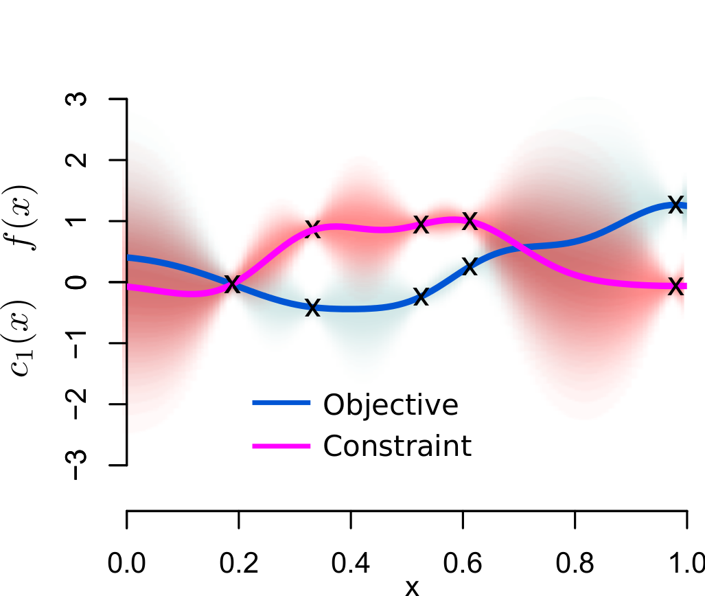
(a) Marginal posteriors

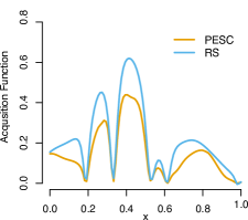
(b) Acquisition functions

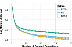
(c) Performance in $1D$

Figure 3: Accuracy of the PESC approximation. (a) Marginal posterior distributions for the objective and constraint given some collected data denoted by $\times$’s. (b) PESC and RS acquisition functions given the data in (a). (c) Median utility gap for PESC, RS and RSDG in the experiments with synthetic functions sampled from the GP prior with $D=1$.

Figure 3(a) shows the posterior distribution for $f$ and $c_{1}$ given 5 observations sampled from the GP prior with ${D=1}$. The posterior is computed using the optimal GP hyperparameters. The corresponding approximations to the acquisition function generated by PESC and RS are shown in Fig. 3(b). In the figure, both PESC and RS use a total of $M=50$ samples from $p(\mathbf{x}_{\star}\,|\,\mathcal{D})$ when approximating the expectation in Eq. 8. The PESC approximation is quite accurate, and importantly its maximum value is very close to the maximum value of the RS approximation. The approximation produced by the version of RS that does not ignore correlations in the samples of $f,c_{1},\ldots,c_{K}$ (not shown) cannot be visually distinguished from the one shown in Fig. 3(b).

One disadvantage of the RS method is its high cost, which scales with the size of the grid used. This grid has to be large to guarantee good performance, especially when $D$ is large. An alternative is to use a small dynamic grid that changes as data is collected. Such a grid can be obtained by sampling from $p(\mathbf{x}_{\star}\,|\,\mathcal{D})$ using the same approach as in PESC to generate these samples (a similar approach is taken by Hennig and Schuler (2012), in which the dynamic grid is sampled from the EI acquisition function). The samples obtained then form the dynamic grid, with the idea that grid points are more concentrated in areas that we expect $p(\mathbf{x}_{\star}\,|\,\mathcal{D})$ to be high. The resulting method is called Rejection Sampling with a Dynamic Grid (RSDG).

We compare the performance of PESC, RS and RSDG in experiments with synthetic data corresponding to 500 pairs of $f$ and $c_{1}$ sampled from the GP prior with ${D=1}$. RS and RSDG draw the same number of samples of $\mathbf{x}_{\star}$ as PESC. We assume that the GP hyper-parameters are known to each method and fix ${\delta=0.05}$, that is, recommendations are made by finding the location with highest posterior mean for $f$ such that $c_{1}$ is non-negative with probability at least ${1-\delta}$. For reporting purposes, we set the utility $u(\mathbf{x})$ of a recommendation $\mathbf{x}$ to be $f(\mathbf{x})$ if $\mathbf{x}$ satisfies the constraint, and otherwise a penalty value of the worst (largest) objective function value achievable in the search space. For each recommendation $\mathbf{x}$, we compute the utility gap $|u(\mathbf{x})-u(\mathbf{x}_{\star})|$, where $\mathbf{x}_{\star}$ is the true solution to the optimization problem. Each method is initialized with the same three random points drawn with Latin hypercube sampling.

Figure 3(c) shows the median of the utility gap for each method for the 500 realizations of $f$ and $c_{1}$. The $x$-axis in this plot is the number of joint function evaluations for $f$ and $c_{1}$. We report the median because the empirical distribution of the utility gap is heavy-tailed and in this case the median is more representative of the location of the bulk of the data than the mean. The heavy tails arise because we are averaging over 500 different optimization problems with very different degrees of difficulty. In this and all of the following experiments, unless otherwise specified, error bars are computed using the bootstrap method. The plot shows that PESC and RS are better than RSDG. Furthermore, PESC is very similar to RS, with PESC even performing slightly better, perhaps because PESC is not confined to a grid as RS is. These results seem to indicate that PESC yields an accurate approximation of the information gain.

6.2 Synthetic Functions in 2 and 8 Input Dimensions

We compare the performance of PESC and RSDG with EIC using the same experimental protocol as in the previous section, but with dimensionalities ${D=2}$ and ${D=8}$. We do not compare with RS here because its use of grids does not scale to higher dimensions. Fig. 4 shows the utility gap for each method across 500 different samples of $f$ and $c_{1}$ from the GP prior with (a) ${D=2}$ and (b) ${D=8}$. Overall, PESC is the best method, followed by RSDG and EIC. RSDG performs similarly to PESC when ${D=2}$, but is significantly worse when ${D=8}$. This shows that, when $D$ is high, grid based approaches (e.g. RSDG) are at a disadvantage with respect to methods that do not require a grid (e.g. PESC).

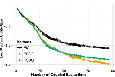
(a) $D=2$

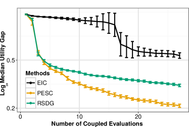
(b) $D=8$

Figure 4: Optimizing samples from the GP prior with (a) $D=2$ and (b) $D=8$.

6.3 A Toy Problem

Next, we compare PESC with EIC and AL (Gramacy et al. (2016), Section 2.4) on the toy problem described by Gramacy et al. (2016), namely,

$$\min_{\mathbf{x}\in[0,1]^{2}}f(\mathbf{x}) \text{ s.t. }c_{1}(\mathbf{x})\geq 0,\,c_{2}(\mathbf{x})\geq 0\,,$$ (23)

$$f(\mathbf{x}) =x_{1}+x_{2}\,,$$

$$c_{1}(\mathbf{x}) =0.5\sin{(2\pi(x_{1}^{2}-2x_{2}))}+x_{1}+2x_{2}-1.5\,,$$

$$c_{2}(\mathbf{x}) =-x_{1}^{2}-x_{2}^{2}+1.5\,.$$

This optimization problem has two local minimizers and one global minimizer. At the global solution, which is at $\mathbf{x}_{\star}\approx[0.1954,0.4404]$, only one of the two constraints ($c_{1}$) is active. Since the objective is linear and $c_{2}$ is not active at the solution, learning about $c_{1}$ is the main challenge of this problem. Fig. 5(a) shows a visualization of the linear objective function and the feasible and infeasible regions, including the location of the global constrained minimizer $\mathbf{x}_{\star}$.

In this case, the evaluations for $f$, $c_{1}$ and $c_{2}$ are noise-free. To produce recommendations in PESC and EIC, we use the confidence value ${\delta=0.05}$. We also use a squared exponential GP kernel. PESC uses $M=10$ samples of $\mathbf{x}_{\star}$ when approximating the expectation in Eq. 8. We use the AL implementation provided by Gramacy et al. (2016) in the R package laGP, which is based on the squared exponential kernel and assumes the objective $f$ is known. Thus, in order for this implementation to be used, AL has an advantage over other methods in that it has access to the true objective function. In all three methods, the GP hyperparameters are estimated by maximum likelihood.

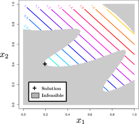
(a) Visualization of the problem.

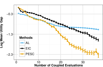
(b) Performance of PESC, AL and EIC.

Figure 5: Comparing PESC, AL, and EIC in the toy problem described by Gramacy et al. (2016). (a) Visualization of the linear objective function and the feasible and infeasible regions. (b) Results obtained by PESC, AL and EIC on the toy problem.

Figure 5(b) shows the mean utility gap for each method across 500 repetitions. Each repetition corresponds to a different initialization of the methods with three data points selected with Latin hypercube sampling. The results show that PESC is significantly better than EIC and AL for this problem. EIC is superior to AL, which performs slightly better at the beginning, possibly because it has access to the ground truth objective $f$.

6.4 Finding a Fast Neural Network

In this experiment, we tune the hyper-parameters of a three-hidden-layer neural network subject to the constraint that the prediction time must not exceed 2 ms on an NVIDIA GeForce GTX 580 GPU (also used for training). We use the Matérn 5/2 kernel for the GP priors. The search space consists of 12 parameters: 2 learning rate parameters (initial value and decay rate), 2 momentum parameters (initial and final values, with linear interpolation), 2 dropout parameters (for the input layer and for other layers), 2 additional regularization parameters (weight decay and max weight norm), the number of hidden units in each of the 3 hidden layers, and the type of activation function (RELU or sigmoid). The network is trained using the deepnet package, and the prediction time is computed as the average time of 1000 predictions for mini-batches of size 128. The network is trained on the MNIST digit classification task with momentum-based stochastic gradient descent for 5000 iterations. The objective is reported as the classification error rate on the standard validation set. For reporting purposes, we treat constraint violations as the worst possible objective value (a classification error of 1.0). This experiment is inspired by a real need for neural networks that can make fast predictions with high accuracy. An example is given by computer vision problems in which the prediction time of the best performing neural network is not fast enough to keep up with the fast rate at which new data is available (e.g., YouTube, connectomics).

Figure 6(a) shows the results of 50 iterations of the Bayesian optimization process. In this experiment and in the next one, the $y$-axis represents the best objective value observed so far, with recommendations produced using ${\delta=0.05}$ and observed constraint violations resulting in objective values equal to 1.0. Curves show averages over five independent experiments. In this case, PESC performs significantly better than EIC.

When the constraints are noisy, reporting the best observation is an overly optimistic metric because the best feasible observation might be infeasible in practice. On the other hand, ground-truth is not available. Therefore, to validate our results further, we used the recommendations made at the final iteration of the Bayesian optimization process for each method (EIC and PESC) and evaluated the functions with these recommended parameters. We repeated the evaluation 10 times for each of the 5 repeated experiments. The result is a ground-truth score obtained as the average of 50 function evaluations. This procedure yields a score of $7.0\pm 0.6\%$ for PESC and $49\pm 4\%$ for EIC (as in the figure, constraint violations are treated as a classification error of $100\%$), where the numbers after the $\pm$ symbol denote the empirical standard deviation. This result is consistent with Fig. 6(a) in that PESC performs significantly better than EIC.

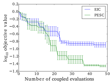
(a) Finding a fast neural network.

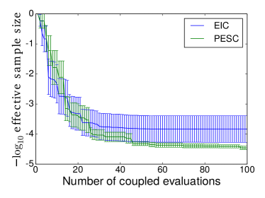
(b) Tuning Hamiltonian Monte Carlo

Figure 6: Results for PESC and EIC on the tuning of machine learning methods with coupled constraints. (a) Tuning a neural network subject to the constraint that it makes predictions in under 2 ms. (b) Tuning Hamiltonian Monte Carlo to maximize the number of effective samples within 5 minutes of compute time, subject to the constraints passing the Geweke and Gelman-Rubin convergence diagnostics and integrator stability.

6.5 Tuning Markov Chain Monte Carlo

Hamiltonian Monte Carlo (HMC) (Duane et al., 1987) is a popular MCMC technique that takes advantage of gradient information for rapid mixing. HMC contains several parameters that require careful tuning. The two basic parameters are the number of leapfrog steps and the step size. HMC may also include a mass matrix which introduces $\mathcal{O}(D^{2})$ additional parameters for problems in $D$ dimensions, although the matrix is often fixed to be diagonal ($D$ parameters) or a multiple of the identity matrix (1 parameter) (Neal, 2011). In this experiment, we optimize the performance of HMC. We use again the Matérn 5/2 kernel for the GP priors. We tune the following parameters: the number of leapfrog steps, the step size, a mass parameter and the fraction of the allotted computation time spent burning in the chain. Our experiment measures the number of effective samples obtained in a fixed computation time. We impose the constraints that the generated samples must pass the Geweke (Geweke, 1992) and Gelman-Rubin (Gelman and Rubin, 1992) convergence diagnostics. In particular, we require the worst (largest absolute value) Geweke test score across all variables and chains to be at most 2.0, and the worst (largest) Gelman-Rubin score between chains and across all variables to be at most 1.2. We use the coda R package (Plummer et al., 2006) to compute the effective sample size and the Geweke convergence diagnostic, and the PyMC python package (Patil et al., 2010) to compute the Gelman-Rubin diagnostic over two independent traces.

The HMC integration may also diverge for large values of the step size. We treat this as a hidden constraint, and set ${\delta=0.05}$. We use HMC to sample from the posterior of a logistic regression binary classification problem using the German credit data set from the UCI repository (Frank and Asuncion, 2010). The data set contains 1000 data points, and is normalized to have zero mean unit variance for each feature. We initialize each chain randomly with ${D=25}$ independent draws from a Gaussian distribution with mean zero and standard deviation $10^{-3}$. For each set of inputs, we compute two chains, each one with five minutes of computation time on a single core of a compute node.

Figure 6(b) compares EIC and PESC on this task, averaged over ten realizations of the experiment. As above, we perform a ground-truth assessment of the final recommendations. For each method (EIC and PESC), we used the recommendations made at the final iteration of the Bayesian optimization process and evaluated the functions with these recommended parameters multiple times. The resulting average effective sample size is $3300\pm 1200$ for PESC and $2300\pm 900$ for EIC, where the number after the $\pm$ symbol denotes the empirical standard deviation. Here, the difference between the two methods is within the margin of error. When we compare these results with the ones in Fig. 6(b) we observe that the latter results are overly optimistic, indicating that this experiment is very noisy. The noise presumably comes from the randomness in the initialization and the execution of HMC, which causes the passing or the failure of the convergence diagnostics to be highly stochastic.

7 Empirical Analyses with Decoupled Functions

Section 6 focused on the evaluation of the performance of PESC in experiments with coupled functions. Here, we evaluate the performance of PESC in the decoupled case, where the different functions can be evaluated independently.

7.1 Accuracy of the PESC Approximation

We first evaluate the accuracy of PESC when approximating the function-specific acquisition functions from LABEL:{eq:individual_acq}. We consider a synthetic problem with input dimension ${D=1}$ and including an objective function and a single constraint function, both drawn from the GP prior distribution. Figure 7(a) shows the marginal posterior distributions for $f$ and $c_{1}$ given 7 observations for the objective and 3 for the constraint. Figures 7(b) and 7(c) show the PESC approximations to the acquisition functions for the objective and the constraint, respectively. These functions approximate how much information we would obtain by the individual evaluation of the objective or the constraint at any given location. We also include in Figs. 7(b) and 7(c) the value of a ground truth obtained by rejection sampling (RS). The RS solution is obtained in the same way as in Section 6.1. Both PESC and RS use a total of $M=50$ samples from $p(\mathbf{x}_{\star}\,|\,\mathcal{D})$. The PESC approximation is quite accurate, and importantly its maximum value is very close to the maximum value of the RS approximation. Figures 7(b) and 7(c) indicate that the highest expected gain of information is obtained by evaluating the constraint at $x\approx 0.3$. The reason for this is that, as Fig. 7(a) shows, the objective is low near $x\approx 0.3$ but the constraint has not been evaluated at that location yet.

Figure 7(d) shows the marginal posterior distributions for $f$ and $c_{1}$ when three more observations have been collected for the constraint. The corresponding approximations given by PESC and RS to the function-specific acquisition functions are shown in Figs. 7(e) and 7(f). As before, the PESC approximation is very similar to the RS one. In this case, evaluating the constraint is no longer as informative as before and the highest expected gain of information is obtained by evaluating the objective at $x\approx 0.25$. Intuitively, as we collect more constraint observations the constraint becomes well determined and the optimizer turns its attention to the objective.

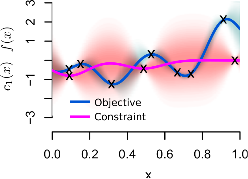
(a) Marginal posteriors

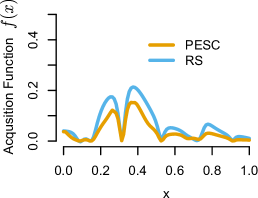
(b) $\alpha_{f}(x)$

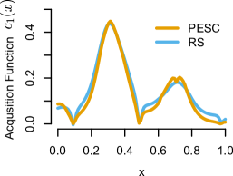
(c) $\alpha_{c}(x)$

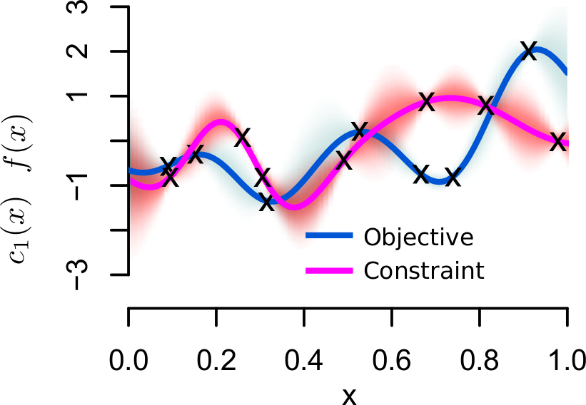
(d) Marginal posteriors

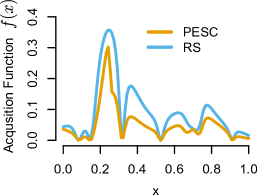
(e) $\alpha_{f}(x)$

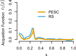
(f) $\alpha_{c}(x)$

Figure 7: Assessing the accuracy of the decoupled PESC approximation for the partial acquisition functions for $\alpha_{f}(x)$ and $\alpha_{c}(x)$. Between the top and bottom rows, three additional observations of the constraint have been made.

7.2 Comparing Coupled and Decoupled PESC

We now compare the performance of coupled and decoupled versions of PESC in the same decoupled optimization problem. This allows us to empirically demonstrate the benefits of treating a decoupled problem as such.

We first consider the toy problem from Section 6.3 given by Eq. 23. We assume that there are three decoupled tasks: one for the objective and another one for each constraint function. We further assume that there is a single resource $r$ with capacity $\omega_{\text{max}}(r)=3$. Each task requires to use resource $r$ for its evaluation and the evaluation of each task takes always the same amount of time, which is assumed to be much larger than the BO computations. At each iteration resource $r$ is used to evaluate 3 functions in parallel. We compare the performance of four versions of PESC, which differ in how they select the 3 parallel evaluations that will be performed at each iteration. The first method is a coupled approach (Coupled) which, at each iteration, evaluates jointly the three tasks at the same input. The second method is a non-competitive decoupling approach (NCD) which, at each iteration, evaluates all the different tasks once but not necessarily at the same input. This is equivalent to assuming that there are 3 resources with capacity 1 and each task can only be evaluated in one resource: the tasks do not have to compete because each one can only be evaluated in its corresponding resource. The third method is a competitive-decoupling approach (CD) which allows the different tasks to compete such that, at each iteration, three not necessarily unique functions are evaluated at three not necessarily unique locations. We also consider an implementation of CD that is not based on PESC and uses the EIC-D approach, as described in Section 2.5. We call this method EIC-CD. EIC-CD works like CD, with the difference that, at each step, we first determine the next evaluation location $\mathbf{x}$ by maximizing the EIC acquisition function. After this, the next task to be evaluated at $\mathbf{x}$ is chosen according to the expected reduction in the entropy of the global feasible minimizer $\mathbf{x}_{\star}$. The original description of this method given by Gelbart et al. (2014) approximates the expected reduction in entropy using Monte Carlo sampling. This is in general computationally very expensive. To speed up EIC-CD, we replace the Monte Carlo sampling step by the approximation of the expected reduction in entropy given by PESC.

All the methods have to update the GP model, the posterior samples of $\mathbf{x}_{\star}$ and the EP solutions just after collecting the data from resource $r$. However, the method CD and EIC-CD have to do two additional update operations after sending the first and the second evaluations to resource $r$, respectively. These updates correspond to step 11 in Algorithm 1 and they allow CD and EIC-CD to condition on pending evaluations that are not complete yet. In our experiments we use the Kriging believer approach, in which we pretend that the pending function evaluations have completed and returned the values of the GP predictive mean at those locations. This allows the methods CD and EIC-CD to update the GP model in a fast way, at the cost of ignoring uncertainty in the predictions of the GP model. The samples of $\mathbf{x}_{\star}$ and the EP solutions are, however, recomputed from scratch once the GP model has been updated. This can be expensive in practice. To address this problem we introduce the method CD-F, which works like CD, but replaces the full updates for the samples of $\mathbf{x}_{\star}$ and the EP solutions with the corresponding fast updates used by PESC-F in Section 5. Therefore, by comparing CD and CD-F, we can evaluate the loss in performance that is obtained by using the fast PESC-F updates. Note that CD-F uses the fast updates only after sending the first and the second evaluations to resource $r$. Once the new data is collected, CD-F uses the original slow updates.

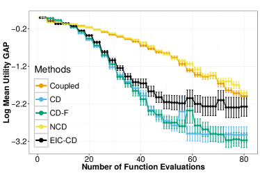
(a) Performance

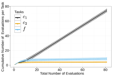
(b) Cumulative task evaluations

Figure 8: Results for the decoupled toy problem (Eq. 23) when using a resource $r$ that can evaluate 3 tasks ($f$, $c_{1}$ or $c_{2}$) in parallel. (a) Performance comparison of Coupled (orange), NCD (yellow), CD (blue), CD-F (green) and EIC-CD (black) approaches. (b) Cumulative number of evaluations for each task performed by CD-F. The algorithm automatically discovers that the constraint $c_{1}$ is much more important than the objective $f$ or the other constraint $c_{2}$.

Figure 8(a) shows the results obtained by each method across 500 repetitions of the experiment starting from random initializations. Recommendations are computed with $\delta=0.01$. The horizontal axis in the plot denotes the number of function evaluations performed so far. Since $\omega_{\text{max}}(r)=3$, these evaluation are performed in parallel in blocks of three. The vertical axis denotes the average utility gap, computed as in Section 6.1. Overall, CD and CD-F perform the best; the fact that CD and CD-F obtain similar results implies that the fast PESC-F updates incur no significant performance loss in this synthetic optimization problem. EIC-CD is worse than these two methods. This is a result of the the sub-optimal two-stage decision process used by EIC-CD to select the next evaluation location and the next task to be evaluated at that location; see Section 2.5 for more details. NCD performs about the same as Coupled which means that, in this problem, the benefits of decoupling come from choosing an unequal distribution of tasks to evaluate, rather than from the additional freedom of evaluating the three tasks at potentially different locations. This hypothesis is corroborated by Fig. 8(b), which shows the average cumulative number of evaluations performed by CD for each task ($f$, $c_{1}$ or $c_{2}$) at each iteration. CD chooses to evaluate the constraint $c_{1}$ far more often than the objective or the other constraint $c_{2}$. This makes sense since the objective is a linear function and $c_{1}$, which has a complicated form, is the only active constraint at the global solution. Thus, the PESC algorithm has automatically discovered that the constraint $c_{1}$ is much more important (both in the sense of being complicated and in the sense of being active at the true solution) than the objective $f$ or the other constraint $c_{2}$. This demonstrates the true power of competitive decoupling, as the algorithm avoids wasting time on uninteresting tasks that might be, in the worst case scenario, even more expensive than the interesting ones.

We perform another comparison of the methods Coupled, NCD and CD-F in synthetic problems in which the objective $f$ and a single constraint function $c_{1}$ are drawn from the GP prior with $D=2$. This is done in the same way as in Section 6.2. We set $\delta=0.05$ and follow an experimental protocol similar to the one from the previous experiment: we assume that there are two tasks, given by $f$ and $c_{1}$, which can be evaluated at a resource $r$ with capacity $\omega_{\text{max}}(r)=2$. Therefore, at any iteration we will be evaluating 2 tasks in parallel. Figure 9(a) shows the median utility gap obtained by each method across 500 different realizations of the experiment. As in the previous toy problem, CD-F outperforms Coupled, while Coupled performs similar to NCD. Again, decoupling is useful when we can choose the tasks to evaluate (CD-F) and evaluating the tasks at potentially different locations (NCD) does not seem to produce significant improvements with respect to the coupled approach.

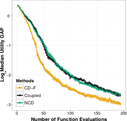
(a) Performance

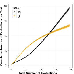
(b) Constraint active

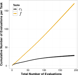
(c) Constraint not active

Figure 9: Results on synthetic problems with $D=2$ sampled from the GP prior as in Section 6.2 when using a resource $r$ that can evaluate 2 tasks ($f$ or $c_{1}$) in parallel. (a) Performance comparison of Coupled (black), NCD (green), and CD-F (orange) approaches. (b) Cumulative number of task evaluations performed by CD-F when $c_{1}$ is active at the solution. (c) Cumulative number of task evaluations performed by CD-F when $c_{1}$ is not active at the solution.

In the previous toy problem, CD-F outperformed NCD and Coupled because it learned that evaluating the constraint $c_{1}$ is much more useful than evaluating the objective $f$ or the constraint $c_{2}$. We perform a similar analysis here by plotting the cumulative number of evaluations for each task performed by CD-F. We divide the 500 realizations into those cases in which the constraint $c_{1}$ is active at the true solution (Fig. 9(b)) and those in which $c_{1}$ is not active at the true solution (Fig. 9(c)). The plots in Figs. 9(b) and 9(c) show that when the constraint $c_{1}$ is active at the solution, CD-F chooses to evaluate $c_{1}$ much more frequently. By contrast, when the constraint is not active, $c_{1}$ is evaluated much less. Presumably, in the latter case $c_{1}$ need only be evaluated until it is determined that it is very unlikely to be active at the solution. After this point, further evaluations of $c_{1}$ are not very informative. These results indicate that the task-specific acquisition functions used by PESC and given by Eq. 14 are able to successfully measure the usefulness of evaluating each different task.

7.3 Performance of PESC-F with Respect to Wall-clock Time

We now evaluate the performance of PESC with fast BO computations (PESC-F, Section 5) while considering the wall-clock time of each experiment. Again, we focus on the toy problem from Section 6.3 given by Eq. 23. To highlight what can go wrong in decoupled optimization problems, we will assume that evaluating the objective is instantaneous, evaluating $c_{1}$ takes 2 seconds, and evaluating $c_{2}$ takes 1 minute. Each of these functions forms a different task so that all of them can be evaluated independently. We also consider that there is a single resource $r$ with $\omega_{\text{max}}(r)=1$, that is, only one task can be evaluated at any given time with no possible parallelism. This setup corresponds to the competitive decoupling scenario from Fig. 1. We limit each experiment time to 15 minutes and consider the following methods: Coupled, and competitive decoupled (CD) with PESC-F and rationality levels $\gamma=\{\infty,1,0.1,0\}$. According to Eq. 22, setting $\gamma=\infty$ is simply another way of saying that fast BO computations are not used.

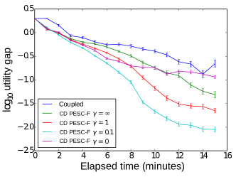
(a) Performance, all approaches

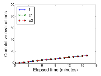
(b) Coupled

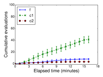
(c) CD PESC-F, $\gamma=\infty$

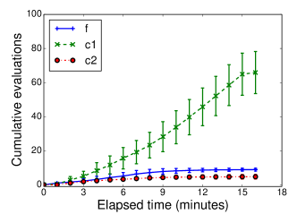
(d) CD PESC-F, $\gamma=1$

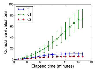
(e) CD PESC-F, $\gamma=0.1$

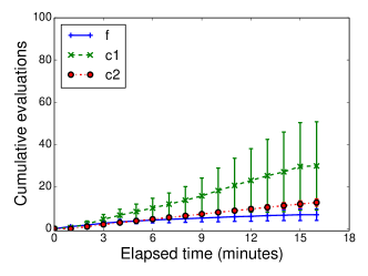
(f) CD PESC-F, $\gamma=0$

Figure 10: Results for Coupled and CD PESC-F with $\gamma=\{\infty,1,0.1,0\}$ on the toy problem given by Eq. 23. Evaluations of $f$ are instantaneous, evaluations of $c_{1}$ take 2 sec. and evaluations of $c_{2}$ take 1 min. The maximum experiment time is 15 min. (a) log utility gap versus wall-clock time. (b-f) Cumulative function evaluations for (b) Coupled, (c) CD PESC-F with $\gamma=\infty$ (no fast computations), (d) CD PESC-F with $\gamma=1.0$, (e) CD PESC-F with $\gamma=0.1$, and (f) CD PESC-F with $\gamma=0$ (no slow computations). Curves reflect the mean over 100 trials. Error bars in (b-f) are given by the empirical standard deviations.

Figure 10(a) shows the average utility gap of each method as a function of elapsed time. The coupled approach is the worst performing one, being outperformed by all the versions of PESC-F with different $\gamma$. This illustrates the advantages of the decoupled approach. The performance of PESC-F is improved as $\gamma$ moves from $\infty$ to $1$ and then to $0.1$. The reason for this is that, as $\gamma$ is reduced, less time is spent in the BO computations and more time is spent in the actual collection of data. However, reducing $\gamma$ too much is detrimental as $\gamma=0$ performs significantly worse than $\gamma=0.1$ and $\gamma=1$. The reason for this is that $\gamma=0$ performs too many fast BO computations, which produce suboptimal decisions.

Figures 10(b), 10(c), 10(d), 10(e), 10(f) and 1 are useful to understand the results obtained by the different methods in Fig. 10(a). These figures show, for each method, the cumulative number of evaluations per task as a function of the elapsed time. The coupled approach performs very few evaluations of the different tasks. The reason for this is that it always evaluates all the tasks the same number of times and this leads to wasting a lot of time by evaluating too often the slowest task, that is, constraint $c_{2}$, which is not very informative about the solution to the problem. The different versions of PESC-F with $\gamma=\{\infty,1,0.1,0\}$ evaluate more often the most informative task, that is, $c_{1}$ and less frequently all the other tasks. As the rationality level $\gamma$ is decreased, less time is spent in the BO computations, and thus more task evaluations are performed. These correspond to increases in performance. However, this trend does not continue indefinitely as $\gamma$ is decreased. When $\gamma=0$, performance is significantly diminished. By not performing slow BO computations, the $\gamma=0$ method is not able to learn that $c_{2}$ is uninformative and continues to spend time evaluating it, thus performing many fewer evaluations of the most informative task $c_{1}$. The configuration files for running this experiment are available at https://github.com/HIPS/Spearmint/tree/PESC/examples/toy-fast-slow.

Table 1 shows the time spent by each method in fast and slow BO computations and in the evaluation of tasks $c_{1}$ and $c_{2}$. We do not include the time spent in the evaluation of task $f$ because it is always zero. Note that the total time spent in the BO computations and in the evaluation of the different tasks does not add up exactly to 15 minutes because, in our implementation, the current iteration is allowed to finish after the 15-minute mark is reached. As expected, the time spent in the BO computations decreases monotonically as $\gamma$ is decreased. The coupled approach spends a small amount of time doing BO computations. The reason for this is that this method does not have to perform step 11 in Algorithm 1 and step 4 is performed less frequently than in the PESC-F methods because Coupled spends most of its time in the evaluation of $c_{2}$.

The fifth column in Table 1 corresponds to the time spent in the evaluation of $c_{1}$. The entries in this column are indicative of the relative performances of each method, since $c_{1}$ is the most important function in this optimization problem. From these entries we may conclude that this problem exhibits an optimal value of $\gamma$ close to $0.1$. This represents an optimal ratio of time spent in the BO computations to time spent in the evaluation of the different tasks. We leave to future work the issue of selecting the optimal value for $\gamma$. In a highly sophisticated approach this could be done in an online fashion by using reinforcement learning.

	Slow BO	Fast BO	Total BO			Total
Method	Comp.	Comp.	Comp.	$c_{1}(\mathbf{x})$	$c_{2}(\mathbf{x})$	Evaluation
Coupled	$2.0$	$0.0$	$2.0$	$0.4$	$13.0$	$13.4$
CD PESC-F, $\gamma=\infty$	$10.2$	$0.0$	$10.2$	$1.4$	$3.6$	$5.0$
CD PESC-F, $\gamma=1$	$5.2$	$3.0$	$8.2$	$2.2$	$4.7$	$6.9$
CD PESC-F, $\gamma=0.1$	$1.5$	$5.1$	$6.6$	$2.5$	$6.0$	$8.5$
CD PESC-F, $\gamma=0.0$	$0.2$	$1.8$	$2.0$	$1.0$	$12.5$	$13.5$

Table 1: Time spent by each method in BO computations and in task evaluations. For each method, the table reports the mean time in minutes, over 100 independent runs, spent in fast and slow BO computations and in the evaluation of tasks $c_{1}$ and $c_{2}$.

8 Conclusions and Future Work

We have presented a general framework for solving Bayesian optimization (BO) problems with unknown constraint functions. In these problems the objective and the constraints can only be evaluated via expensive queries to black boxes that may provide noisy values. Our framework allows for problems in which the objective and the constraints can be split into subsets of functions that require coupled evaluation, meaning that these functions have always to be jointly evaluated at the same input. We call these subsets of coupled functions tasks. Different tasks may, however, be evaluated independently at different locations, that is, in a decoupled way. Furthermore, the tasks may or may not compete for a limited set of resources during their evaluation. Based on this, we have then introduced the notions of competitive decoupling (CD), where two or more tasks compete for the same resource, and non-competitive decoupling (NCD), where the tasks require to use different resources and can therefore be evaluated in parallel. The notion of parallel BO is a special case in which one task requires a specific resource, of which many instances are available. We have then presented a general procedure, given by Algorithm 1, to solve problems with an arbitrary combination of coupling and decoupling. This algorithm receives as input a bipartite graph $\mathcal{G}$ whose nodes are resources and tasks and whose edges connect each task with the resource at which it can be evaluated. Algorithm 1 relies on an acquisition function that can measure the utility of evaluating any arbitrary subset of functions, that is, of any possible task. An acquisition function that satisfies this requirement is said to be separable.

To implement Algorithm 1, we have proposed a new information-based approach called Predictive Entropy Search with Constraints (PESC). At each iteration, PESC collects data at the location that is expected to provide the highest amount of information about the solution to the optimization problem. By introducing a factorization assumption, we obtain an acquisition function that is additive over the subset of functions to be evaluated. That is, the amount of information that we approximately gain by jointly evaluating a set of functions is equal to the sum of the gains of information that we approximately obtain by the individual evaluation of each of the functions. This property means that the acquisition function of PESC is separable. Therefore, PESC can be used to solve general constrained BO problems with decoupled evaluation, something that has not been previously addressed.

We evaluated the performance of PESC in coupled problems, where all the functions (objective and constraints) are always jointly evaluated at the same input location. This is the standard setting considered by most prior approaches to constrained BO. The results of our experiments show that PESC achieves state-of-the-art results in this scenario. We also evaluated the performance of PESC in the decoupled setting, where the different tasks can be evaluated independently at arbitrary input locations. We considered scenarios with competition (CD) and with non-competition (NCD) and compared the performances of two versions of PESC: one with decoupling (decoupled PESC) and another one that always performs coupled evaluations (coupled PESC). Decoupled PESC is significantly better than coupled PESC when there is competition, that is, in the CD setting. The reason for this is that some functions can be more informative than others and decoupled PESC exploits this to make optimal decisions when deciding which function to evaluate next with limited resources. In particular, decoupled PESC avoids wasting time in function evaluations that are unlikely to improve the current estimate of the solution to the optimization problem. However, when there is no competition, that is, in the NCD setting, coupled and decoupled PESC perform similarly. Therefore, in our experiments, the main advantages of considering decoupling seem to come from choosing an unequal distribution of tasks to evaluate, rather than from the additional freedom of evaluating the different tasks at potentially arbitrary locations. In our experiments we have assumed that the evaluation of all the functions takes the same amount of time. However, NCD is expected to perform better than the coupled approach in other settings in which some functions are much faster to evaluate than others. Evaluating the performance of NCD in these settings is left as future work.

For the BO approach to be useful, the time spent performing BO computations (such as computing and globally optimizing the acquisition function) has to be significantly shorter than the time spent collecting data. However, decoupled optimization problems may include some tasks that are fast to evaluate. When these tasks are informative and their evaluation time is comparable to that of the BO computations, the BO approach may be inefficient. To address this issue, we follow a bounded rationality approach and introduce additional approximations in the computations made by PESC to reduce their cost when necessary. The new method is called PESC-F and it is able to automatically switch between fast, but approximate, and slow, but accurate, operations. A parameter called the rationality level is used in PESC-F to balance the amount of time that is spent in the BO computations and in the actual collection of data. Experiments with wall-clock time in a CD scenario show that PESC-F can be significantly better than the original version of PESC.

In summary, PESC is an effective algorithm for BO problems with unknown constraints and the separability of its acquisition function makes it a promising direction towards a unified solution for constrained BO problems. As new acquisition functions are proposed in the future, they will hopefully be developed with separability in mind as an important and desirable property.

The code for PESC, including decoupling and PESC-F, is available in PESC branch of the open-source Bayesian optimization package Spearmint at https://github.com/HIPS/Spearmint/tree/PESC.

One potential line of future work includes extensions to settings where tasks require more than one resource to run. This could, for example, be formalized using a framework similar to the one presented in Section 3, but where the resource dependencies for each task $t$ are represented as a set of edges $\mathcal{E}_{ti}=\{t\sim r\}$ for the $i$th potential allocation of resources. This can be interpreted as the statement that all resource nodes $\mathcal{V}_{ti}=\{r:(t\sim r)\in\mathcal{E}_{ti}\}$ are required in order to initiate task $t$ using allocation $i$. Note that the union of these edges now specifies a multigraph with edges $\mathcal{E}=\bigcup_{t,i}\mathcal{E}_{ti}$ due to the fact there may be resources that are required across multiple allocations of a particular task. This also modifies the pseudocode for Algorithm 1 where the loop over resources $r$ becomes a loop over potential allocations such that $\omega(r)<\omega_{\text{max}}(r)$ for $r\in\mathcal{V}_{ti}$ for some $(t,i)$ pair. In the case where each task requires only a single resource this reduces to the earlier formulation. Another possibility is for allocations where the resources are time or iteration dependent. This would require some form of temporal planning. To make such a procedure feasible, however, it may be necessary to consider greedy decisions at each point in time.

Another direction for future work is concerned with the use of bounded rationality in Bayesian optimization. Here we have used a simple heuristic for selecting between two levels (fast and slow) of computations in PESC-F. However, we could consider a larger number of levels with increasingly more accurate computations (Hay et al., 2012). The Bayesian optimization algorithm would then have to optimally select one of these to determine the next evaluation location. We could also consider different modeling approaches for the collected data, with different trade-offs between accuracy and computational cost. We also leave for future work a theoretical analysis of PESC. This would be in the line of the work of Russo and Van Roy (2014) on information-directed sampling. However, they use simpler models for the data and do not consider problems with constraints.

Finally, we would like to point out that the approach described here can be applied in a straightforward manner to address multi-objective Bayesian optimization problems (Knowles, 2006). In the multi-objective case the different tasks would be given by groups of objective functions that have to be evaluated in a coupled manner. An extension of PES for working with multiple objectives is given by Hernández-Lobato et al. (2016).

Acknowledgments

José Miguel Hernández-Lobato acknowledges support from the Rafael del Pino Foundation. Zoubin Ghahramani acknowledges support from Google Focused Research Award and EPSRC grant EP/I036575/1. Matthew W. Hoffman acknowledges support from EPSRC grant EP/J012300/1.

A The Expectation Propagation Method Used by PESC

We describe here the expectation propagation (EP) method that is used by PESC to adjust a Gaussian approximation to the non-Gaussian factor $f(\mathbf{f},\mathbf{c}_{1},\ldots,\mathbf{c}_{K}|\mathbf{x}_{\star}^{j})$ in Eq. 17. This is done after replacing the infinite set $\mathcal{X}$ with the finite set $\mathcal{Z}$, which contains only the locations at which the objective $f$ has been evaluated so far, the value of $\mathbf{x}_{\star}^{j}$ and $\mathbf{x}$. Recall that $\mathbf{x}$ is the input to the acquisition function, that is, it contains the location at which we are planning to evaluate $f,c_{1},\ldots,c_{K}$. When $\mathcal{X}$ is replaced with $\mathcal{Z}$ we have that the vectors $\mathbf{f},\mathbf{c}_{1},\ldots,\mathbf{c}_{K}$ contain now the result of the noise-free evaluations of $f,c_{1},\ldots,c_{K}$ at $\mathcal{Z}$, that is,

$$\mathbf{f} =[f(\mathbf{x}_{f}^{1}),\ldots,f(\mathbf{x}_{f}^{N_{1}}),f(\mathbf{x}_{\star}^{j}),f(\mathbf{x})]^{\text{T}}\,,$$ (24)

$$\mathbf{c}_{k} =[c_{k}(\mathbf{x}_{f}^{1}),\ldots,c_{k}(\mathbf{x}_{f}^{N_{1}}),c_{k}(\mathbf{x}_{\star}^{j}),c_{k}(\mathbf{x})]^{\text{T}}\,,\quad\text{for }\quad k=1,\ldots,K\,.$$ (25)

where $\mathbf{x}_{f}^{1},\ldots,\mathbf{x}_{f}^{N_{1}}$ are the locations at which the objective $f$ has been evaluated so far. That is, the first $N_{1}$ entries in $\mathbf{f},\mathbf{c}_{1},\ldots,\mathbf{c}_{K}$ contain the function values at the locations for which there is data for the objective. These entries are then followed by the function values at $\mathbf{x}_{\star}^{j}$ and at $\mathbf{x}$. When we replace $\mathcal{X}$ with $\mathcal{Z}$ we have that

$$f(\mathbf{f},\mathbf{c}_{1},\ldots,\mathbf{c}_{K}|\mathbf{x}_{\star}^{j})=p(\mathbf{f},\mathbf{c}_{1},\ldots,\mathbf{c}_{K}|\mathcal{D})\Gamma(\mathbf{x}_{\star}^{j})\left\{\prod_{i=1}^{N_{1}}\Psi(\mathbf{x}_{f}^{i})\right\}\Psi(\mathbf{x})\,.$$ (26)

In this expression we should have included a factor $\Psi(\mathbf{x}_{\star}^{j})$ since $\mathbf{x}_{\star}^{j}\in\mathcal{Z}$. We ignore such factor because it is always equal to 1 according to Eq. 16. In Eq. 26 we have separated the non-Gaussian factor that depends on $\mathbf{x}$, that is, $\Psi(\mathbf{x})$ from those factors that do not depend on $\mathbf{x}$, that is, $\Gamma(\mathbf{x}_{\star}^{j}),\Psi(\mathbf{x}_{f}^{1}),\ldots,\Psi(\mathbf{x}_{f}^{N_{1}})$. All these non-Gaussian factors are approximated with Gaussians using EP.

Finding the next suggestion involves maximizing the acquisition function. This requires to evaluate the acquisition function at many different $\mathbf{x}$ and recomputing the complete EP approximation for each value of $\mathbf{x}$ can be excessively expensive. To avoid this, we first compute the EP approximation for the factors that do not depend on $\mathbf{x}$ in isolation, store it and then reuse it as we compute the EP approximation for the remaining factors. Since most of the factors do not depend on $\mathbf{x}$, this leads to large speedups when we have to evaluate the acquisition function at many different $\mathbf{x}$. Therefore, we start by finding a Gaussian approximation to the factors that do not depend on $\mathbf{x}$, that is, $\Gamma(\mathbf{x}_{\star}^{j}),\Psi(\mathbf{x}_{f}^{1}),\ldots,\Psi(\mathbf{x}_{f}^{N_{1}})$, while ignoring the other factor that does depend on $\mathbf{x}$, that is, $\Psi(\mathbf{x})$.

A.1 Approximating the Non-Gaussian Factors that do not Depend on $\mathbf{x}$

We use EP to find a Gaussian approximation to $\Gamma(\mathbf{x}_{\star}^{j}),\Psi(\mathbf{x}_{f}^{1}),\ldots,\Psi(\mathbf{x}_{f}^{N_{1}})$ in Eq. 26 when $\Psi(\mathbf{x}_{1}),\ldots,\Psi(\mathbf{x}_{K+1})$ are assumed to be constant and equal to 1. Because the data is assumed to be generated from independent GPs, we have that $p(\mathbf{f},\mathbf{c}_{1},\ldots,\mathbf{c}_{K}|\mathcal{D})$ in Eq. 26 is

$$p(\mathbf{f},\mathbf{c}_{1},\ldots,\mathbf{c}_{K}|\mathcal{D})=\mathcal{N}(\mathbf{f}\,|\,\mathbf{m}_{1}^{\text{pred}},\mathbf{V}_{1}^{\text{pred}})\prod_{k=1}^{K}\left\{\mathcal{N}(\mathbf{c}_{k}\,|\,\mathbf{m}_{k+1}^{\text{pred}},\mathbf{V}_{k+1}^{\text{pred}})\right\}\,,$$ (27)

where $\mathbf{m}^{\text{pred}}_{1}$ and $\mathbf{V}^{\text{pred}}_{1}$ are the mean and covariance matrix of the posterior distribution of $\mathbf{f}$ given the data for the objective and $\mathbf{m}^{\text{pred}}_{k+1}$ and $\mathbf{V}^{\text{pred}}_{k+1}$ are the mean and covariance matrix of the posterior distribution of $\mathbf{c}_{k}$ given the data for constraint $k$. In particular, from Eqs. (2.22) to (2.24) of (Rasmussen and Williams, 2006) we have that

$$\mathbf{m}^{\text{pred}}_{i} =\mathbf{K}_{\star}^{i}(\mathbf{K}^{i}+\nu_{i}\mathbb{I})^{-1}\mathbf{y}^{i}\,,$$ (28)

$$\mathbf{V}^{\text{pred}}_{i} =\mathbf{K}_{\star,\star}^{i}-\mathbf{K}_{\star}^{i}(\mathbf{K}^{i}+\nu_{i}\mathbb{I})^{-1}[\mathbf{K}_{\star}^{i}]^{\top}\,,\quad\text{for}\quad i=1,\ldots,K+1\,,$$ (29)

where $\mathbf{y}^{i}$ is an $N_{i}$-dimensional vector with the data for the $i$-th function in $\{f,c_{1},\ldots,c_{K}\}$, $\mathbf{K}_{\star}^{i}$ is an $(N_{1}+2)\times N_{i}$ matrix with the prior cross-covariances between the entries of the $i$-th vector in $\{\mathbf{f},\mathbf{c}_{1},\ldots,\mathbf{c}_{K}\}$ and the value of the corresponding function at the locations for which there is data available for that function and $\mathbf{K}_{\star,\star}^{i}$ is an $(N_{1}+2)\times(N_{1}+2)$ matrix with the prior covariances between entries of the $i$-th vector in $\{\mathbf{f},\mathbf{c}_{1},\ldots,\mathbf{c}_{K}\}$ and $\nu_{i}$ is the noise variance at the black-box for the $i$-th function in $\{f,c_{1},\ldots,c_{K}\}$.

The exact factors $\Gamma(\mathbf{x}_{\star}^{j}),\Psi(\mathbf{x}_{f}^{1}),\ldots,\Psi(\mathbf{x}_{f}^{N_{1}})$ from Eq. 26 are then approximated with the corresponding Gaussian factors $\widetilde{\Gamma}(\mathbf{x}_{\star}^{j}),\widetilde{\Psi}(\mathbf{x}_{f}^{1}),\ldots,\widetilde{\Psi}(\mathbf{x}_{f}^{N_{1}})$. Let $\bm{\beta}_{n}(\mathbf{f})=[f(\mathbf{x}_{f}^{n}),f(\mathbf{x}_{\star}^{j})]^{\text{T}}$, where $\mathbf{x}_{f}^{n}$ is the $n$-th location for which there is data for the objective $f$. Then, we define

where $\widetilde{\mathbf{A}}_{n}$ and $\widetilde{\mathbf{b}}_{n}$ are the natural parameters of a bivariate Gaussian distribution on $\bm{\beta}_{n}(\mathbf{f})$ and $\widetilde{d}_{n}^{k}$ and $\widetilde{e}_{n}^{k}$ are the natural parameters of a Gaussian distribution on $c_{k}(\mathbf{x}_{f}^{n})$, that is, the value of constraint $k$ at the $n$-th location for which there is data for the objective. We also define

$$\widetilde{\Gamma}(\mathbf{x}_{\star}^{j})\propto\prod_{k=1}^{K}\exp\left\{-\frac{1}{2}c_{k}(\mathbf{x}_{\star}^{j})^{2}\widetilde{g}_{k}+c_{k}(\mathbf{x}_{\star}^{j})\widetilde{h}_{k}\right\}\,,$$

where $\widetilde{g}_{k}$ and $\widetilde{h}_{k}$ are the natural parameters of a Gaussian distribution on $c_{k}(\mathbf{x}_{\star}^{j})$, that is, the value of constraint $k$ at the current posterior sample of $\mathbf{x}_{\star}$.

The parameters $\widetilde{\mathbf{A}}_{n}$, $\widetilde{\mathbf{b}}_{n}$, $\widetilde{d}_{n}^{k}$, $\widetilde{e}_{n}^{k}$, $\widetilde{g}_{k}$ and $\widetilde{h}_{k}$ are fixed by running EP. Once the value of these parameters has been fixed, we replace the exact factors $\Gamma(\mathbf{x}_{\star}^{j}),\Psi(\mathbf{x}_{f}^{1}),\ldots,\Psi(\mathbf{x}_{f}^{N_{1}})$ in Eq. 26 with their corresponding Gaussian approximations to obtain an approximation to $f(\mathbf{f},\mathbf{c}_{1},\ldots,\mathbf{c}_{K}|\mathbf{x}_{\star}^{j})$. We denote this approximation by $q(\mathbf{f},\mathbf{c}_{1},\ldots,\mathbf{c}_{K})$, where

$$q(\mathbf{f},\mathbf{c}_{1},\ldots,\mathbf{c}_{K})\propto p(\mathbf{f},\mathbf{c}_{1},\ldots,\mathbf{c}_{K}|\mathcal{D})\widetilde{\Gamma}(\mathbf{x}_{\star}^{j})\left\{\prod_{i=1}^{N_{1}}\widetilde{\Psi}(\mathbf{x}_{f}^{i})\right\}\left\{\prod_{k=1}^{K+1}\widetilde{\Psi}(\mathbf{x}_{k})\right\}\,.$$ (31)

Since the approximate factors are Gaussian and $p(\mathbf{f},\mathbf{c}_{1},\ldots,\mathbf{c}_{K}|\mathcal{D})$ is also Gaussian, we have that $q(\mathbf{f},\mathbf{c}_{1},\ldots,\mathbf{c}_{K})$ is also Gaussian:

$$q(\mathbf{f},\mathbf{c}_{1},\ldots,\mathbf{c}_{K})=\mathcal{N}(\mathbf{f}|\mathbf{m}_{1},\mathbf{V}_{1})\prod_{k=1}^{K}\mathcal{N}(\mathbf{c}_{k}|\mathbf{m}_{k+1},\mathbf{V}_{k+1})\,,$$ (32)

where, by applying the formula for products of Gaussians, we obtain

$$\mathbf{V}_{i} =\left[[\mathbf{V}^{\text{pred}}_{i}]^{-1}+\widetilde{\mathbf{S}}_{i}\right]^{-1}\,,$$ (33)

$$\mathbf{m}_{i} =\mathbf{V}_{i}\left[[\mathbf{V}^{\text{pred}}_{i}]^{-1}\mathbf{m}^{\text{pred}}_{i}+\widetilde{\mathbf{t}}_{i}\right]\,,\quad\text{for}\quad i=1,\ldots,K+1\,,$$ (34)

with the following definitions for $\widetilde{\mathbf{S}}_{i}$ and $\widetilde{\mathbf{t}}_{i}$:

• $\widetilde{\mathbf{S}}_{1}$ is an $(N_{1}+2)\times(N_{1}+2)$ matrix whose non-zero entries are

  • $[\widetilde{\mathbf{S}}_{1}]_{n,n}=\left[\mathbf{A}_{n}\right]_{1,1}$ for $n=1,\ldots,N_{1}\,$,

  • $[\widetilde{\mathbf{S}}_{1}]_{N_{1}+1,n}=[\widetilde{\mathbf{S}}_{1}]_{n,N_{1}+1}=\left[\mathbf{A}_{n}\right]_{1,2}$ for $n=1,\ldots,N_{1}\,$,

  • $[\widetilde{\mathbf{S}}_{1}]_{N+1,N+1}=\sum_{n=1}^{N_{1}}\left[\mathbf{A}_{n}\right]_{2,2}\,$.

• $\widetilde{\mathbf{S}}_{k+1}$, for $k=1,\ldots,K$, is an $(N_{1}+2)\times(N_{1}+2)$ matrix whose non-zero entries are

  • $[\widetilde{\mathbf{S}}_{k+1}]_{n,n}=d_{n}$ for $n=1,\ldots,N_{1}\,$,

  • $[\widetilde{\mathbf{S}}_{k+1}]_{N_{1}+1,N_{1}+1}=g_{n}$ for $n=1,\ldots,N_{1}\,$.

• $\widetilde{\mathbf{t}}_{1}$ is an $(N_{1}+2)$-dimensional vector whose non-zero entries are

  • $[\widetilde{\mathbf{t}}_{1}]_{n}=[\widetilde{\mathbf{b}}_{n}]_{1}$ for $n=1,\ldots,N_{1}\,$,

  • $[\widetilde{\mathbf{t}}_{1}]_{N_{1}+1}=\sum_{n=1}^{N_{1}}[\widetilde{\mathbf{b}}_{n}]_{2}\,$.

• $\widetilde{\mathbf{t}}_{k+1}$, for $k=1,\ldots,K$, is an $(N_{1}+2)$-dimensional vector whose non-zero entries are

  • $[\widetilde{\mathbf{t}}_{k+1}]_{n}=\widetilde{e}_{n}^{k}$ for $n=1,\ldots,N_{1}\,$,

  • $[\widetilde{\mathbf{t}}_{k+1}]_{N_{1}+1}=\widetilde{h}_{k}\,$.

We now explain how to obtain the values of all the $\widetilde{\mathbf{A}}_{n}$, $\widetilde{\mathbf{b}}_{n}$, $\widetilde{d}_{n}^{k}$, $\widetilde{e}_{n}^{k}$, $\widetilde{g}_{k}$ and $\widetilde{h}_{k}$ using EP.

A.1.1 Adjusting $\widetilde{\Psi}(\mathbf{x}_{f}^{n})$ by EP

We explain how to adjust the parameters $\widetilde{\mathbf{A}}_{n}$, $\widetilde{\mathbf{b}}_{n}$, $\widetilde{d}_{n}^{k}$ and $\widetilde{e}_{n}^{k}$ of the approximate factor $\widetilde{\Psi}(\mathbf{x}_{f}^{n})$ using EP. EP performs this operation by minimizing the following Kullback-Leibler divergence:

$$\text{KL}[\Psi(\mathbf{x}_{f}^{n})q^{\neg n}(\mathbf{f},\mathbf{c}_{1},\ldots,\mathbf{c}_{K})||\widetilde{\Psi}(\mathbf{x}_{f}^{n})q^{\neg n}(\mathbf{f},\mathbf{c}_{1},\ldots,\mathbf{c}_{K})]\,,$$ (35)

where $q^{\neg n}(\mathbf{f},\mathbf{c}_{1},\ldots,\mathbf{c}_{K})$ is the cavity distribution given by

$$q^{\neg n}(\mathbf{f},\mathbf{c}_{1},\ldots,\mathbf{c}_{K})=q(\mathbf{f},\mathbf{c}_{1},\ldots,\mathbf{c}_{K})[\widetilde{\Psi}(\mathbf{x}_{f}^{n})]^{-1}\,,$$ (36)

If we marginalize out all variables except those which $\widetilde{\Psi}(\mathbf{x}_{f}^{n})$ depends on, namely $\bm{\beta}_{n}(\mathbf{f})$ and $c_{1}(\mathbf{x}_{f}^{n}),\ldots,c_{K}(\mathbf{x}_{f}^{n})$, then $q^{\neg n}$ takes the form

$$q^{\neg n}[\bm{\beta}_{n}(\mathbf{f}),c_{1}(\mathbf{x}_{f}^{n}),\ldots,c_{K}(\mathbf{x}_{f}^{n})]\propto\mathcal{N}(\bm{\beta}_{n}(\mathbf{f})\,|\,\mathbf{b}^{\neg n},\mathbf{A}^{\neg n})\left\{\prod_{k=1}^{K}\mathcal{N}(c_{k}(\mathbf{x}_{f}^{n})\,|\,e^{\neg n}_{k},d^{\neg n}_{k})\right\}\,,$$ (37)

where the parameters $\mathbf{b}^{\neg n}$, $\mathbf{A}^{\neg n}$, $e^{\neg n}_{k}$ and $d^{\neg n}_{k}$ of these Gaussian distributions are obtained from the ratio of $q$ and $\widetilde{\Psi}(\mathbf{x}_{f}^{n})$ by using the formula for dividing Gaussians:

$$\mathbf{A}^{\neg n} =\left\{\mathbf{V}_{\bm{\beta}_{n}(\mathbf{f})}^{-1}-\widetilde{\mathbf{A}}_{n}\right\}^{-1}\,, \mathbf{b}^{\neg n} =\mathbf{A}^{\neg n}\left\{\mathbf{V}_{\bm{\beta}_{n}(\mathbf{f})}^{-1}\mathbf{m}_{\bm{\beta}_{n}(\mathbf{f})}-\widetilde{\mathbf{b}}_{n}\right\}\,,$$ (38)

$$d^{\neg n}_{k} =\left\{v_{c_{k}(\mathbf{x}_{f}^{n})}^{-1}-\widetilde{d}_{k}\right\}^{-1}\,, e^{\neg n}_{k} =d^{\neg n}_{k}\left\{v_{c_{k}(\mathbf{x}_{f}^{n})}^{-1}m_{c_{k}(\mathbf{x}_{f}^{n})}-\widetilde{e}_{k}\right\}^{-1}\,,$$ (39)

where $\mathbf{V}_{\bm{\beta}_{n}(\mathbf{f})}$ is the $2\times 2$ covariance matrix for $\bm{\beta}_{n}(\mathbf{f})$ given by $q(\mathbf{f},\mathbf{c}_{1},\ldots,\mathbf{c}_{K})$ in Eq. 32, $\mathbf{m}_{\bm{\beta}_{n}(\mathbf{f})}$ is the corresponding $2$-dimensional mean vector, $v_{c_{k}(\mathbf{x}_{f}^{n})}$ is the variance for $c_{k}(\mathbf{x}_{f}^{n})$ given by $q(\mathbf{f},\mathbf{c}_{1},\ldots,\mathbf{c}_{K})$ in Eq. 32 and $m_{c_{k}(\mathbf{x}_{f}^{n})}$ is the corresponding mean parameter.

To minimize Eq. 35 we match the 1st and 2nd moments of $\Psi(\mathbf{x}_{f}^{n})q^{\neg n}(\mathbf{f},\mathbf{c}_{1},\ldots,\mathbf{c}_{K})$ and $\widetilde{\Psi}(\mathbf{x}_{f}^{n})q^{\neg n}(\mathbf{f},\mathbf{c}_{1},\ldots,\mathbf{c}_{K})]$. The moments of $\Psi(\mathbf{x}_{f}^{n})q^{\neg n}(\mathbf{f},\mathbf{c}_{1},\ldots,\mathbf{c}_{K})$ can be obtained from the derivatives of the logarithm of its normalization constant $Z$, which is given by

where $\alpha_{n}^{k}=m_{c_{k}(\mathbf{x}_{f}^{n})}v_{c_{k}(\mathbf{x}_{f}^{n})}^{-1/2}$ and $\alpha_{n}=[1,\,-1]\mathbf{m}_{\bm{\beta}_{n}(\mathbf{f})}([1,\;-1]\mathbf{V}_{\bm{\beta}_{n}(\mathbf{f})}[1,\,-1]^{\top})^{-1/2}$ and $\Phi$ is the standard Gaussian cdf. We follow Eqs. (5.12) and (5.13) in (Minka, 2001b) to update $\widetilde{d}_{n}^{k}$ and $\widetilde{e}_{n}^{k}$ in Eq. 30. However, we use the second partial derivative with respect to $e^{\neg n}_{k}$ rather than first partial derivative with respect to $d^{\neg n}_{k}$ for numerical robustness. These derivatives are given by

$$\frac{\partial\log Z}{\partial e^{\neg n}_{k}} =\frac{(Z-1)\phi(\alpha_{n}^{k})}{Z\Phi(\alpha_{n}^{k})\sqrt{d^{\neg n}_{k}}}\,, \frac{\partial^{2}\log Z}{\partial[e^{\neg n}_{k}]^{2}} =-\frac{\partial\log Z}{\partial e^{\neg n}_{k}}\cdot\frac{\alpha_{n}^{k}}{\sqrt{d^{\neg n}_{k}}}-\left[\frac{\partial\log Z}{\partial e^{\neg n}_{k}}\right]^{2}\,,$$ (41)

where $\phi$ is the standard Gaussian pdf. The update equations for the parameters $\widetilde{d}_{n}^{k}$ and $\widetilde{e}_{n}^{k}$ of the approximate factor $\widetilde{\Psi}(\mathbf{x}_{f}^{n})$ are then

(42)

We now perform the analogous operations to update $\widetilde{\mathbf{A}}_{n}$ and $\widetilde{\mathbf{b}}_{n}$. We need to compute

$$\frac{\partial\log Z}{\partial\mathbf{b}^{\neg n}} =\frac{\left\{\prod_{k=1}^{K}\Phi[\alpha_{n}^{k}]\right\}\phi(\alpha_{n})}{Z\sqrt{s}}[1,\,-1]\,,$$ (43)

$$\frac{\partial\log Z}{\partial\mathbf{A}^{\neg n}} =-\frac{1}{2}[1,\,-1]^{\top}[1,\,-1]\frac{\left\{\prod_{k=1}^{K}\Phi[\alpha_{n}^{k}]\right\}\phi(\alpha_{n})\alpha_{n}}{Zs}\,,$$ (44)

where $s=[-1,\,1]\mathbf{A}^{\neg n}[-1,\,1]^{\top}$. We then compute the mean vector and covariance matrix for $\bm{\beta}_{n}(\mathbf{f})$ with respect to $\Psi(\mathbf{x}_{f}^{n})q^{\neg n}(\mathbf{f},\mathbf{c}_{1},\ldots,\mathbf{c}_{K})$:

$$[\mathbf{V}_{\bm{\beta}_{n}(\mathbf{f})}]_{\text{new}} =\mathbf{A}^{\neg n}-\mathbf{A}^{\neg n}\left[\frac{\partial\log Z}{\partial\mathbf{b}^{\neg n}}\left(\frac{\partial\log Z}{\partial\mathbf{b}^{\neg n}}\right)^{\top}-2\frac{\partial\log Z}{\partial\mathbf{A}^{\neg n}}\right]\mathbf{A}^{\neg n}\,,$$ (45)

$$[\mathbf{m}_{\bm{\beta}_{n}(\mathbf{f})}]_{\text{new}} =\mathbf{b}^{\neg n}+\mathbf{A}^{\neg n}\frac{\partial\log Z}{\partial\mathbf{b}^{\neg n}}\,.$$ (46)

Next, we divide the Gaussian with mean and covariance parameters given by Eqs. 45 and 46 by the marginal for $\bm{\beta}(\mathbf{f})$ in the cavity distribution $q^{\neg n}(\mathbf{f},\mathbf{c}_{1},\ldots,\mathbf{c}_{K})$. Therefore, the new parameters $\widetilde{\mathbf{A}}_{n}$ and $\widetilde{\mathbf{b}}_{n}$ of the approximate factor $\widetilde{\Psi}(\mathbf{x}_{f}^{n})$ are obtained using the formula for the ratio of two Gaussians:

$$\widetilde{\mathbf{A}}_{n}^{\text{new}} =[\mathbf{V}_{\bm{\beta}_{n}(\mathbf{f})}]_{\text{new}}^{-1}-\left[\mathbf{A}^{\neg n}\right]^{-1}\,,$$ (47)

$$\widetilde{\mathbf{b}}_{n}^{\text{new}} =[\mathbf{V}_{\bm{\beta}_{n}(\mathbf{f})}]_{\text{new}}^{-1}[\mathbf{m}_{\bm{\beta}_{n}(\mathbf{f})}]_{\text{new}}-\left[\mathbf{A}^{\neg n}\right]^{-1}\mathbf{b}^{\neg n}\,.$$ (48)

A.1.2 Adjusting $\widetilde{\Gamma}(\mathbf{x}_{\star}^{j})$ by EP

We explain how to adjust the parameters $\widetilde{g}_{k}$ and $\widetilde{h}_{k}$ of the approximate factor $\widetilde{\Gamma}(\mathbf{x}_{\star}^{j})$ using EP. EP performs this operation by minimizing the following Kullback-Leibler divergence:

$$\text{KL}[\Gamma(\mathbf{x}_{\star}^{j})q^{\neg}(\mathbf{f},\mathbf{c}_{1},\ldots,\mathbf{c}_{K})||\widetilde{\Gamma}(\mathbf{x}_{\star}^{j})q^{\neg}(\mathbf{f},\mathbf{c}_{1},\ldots,\mathbf{c}_{K})]\,,$$ (49)

where $q^{\neg}(\mathbf{f},\mathbf{c}_{1},\ldots,\mathbf{c}_{K})$ is the cavity distribution given by

$$q^{\neg}(\mathbf{f},\mathbf{c}_{1},\ldots,\mathbf{c}_{K})=q(\mathbf{f},\mathbf{c}_{1},\ldots,\mathbf{c}_{K})[\widetilde{\Gamma}(\mathbf{x}_{\star}^{j})]^{-1}\,,$$ (50)

We integrate out in $q^{\neg}$ all the variables except those which $\widetilde{\Gamma}(\mathbf{x}_{\star}^{j})$ does depend on, namely, $c_{1}(\mathbf{x}_{\star}^{j}),\ldots,c_{K}(\mathbf{x}_{\star}^{j})$. Then $q^{\neg}$ takes the form

$$q^{\neg}[c_{1}(\mathbf{x}_{\star}^{j}),\ldots,c_{K}(\mathbf{x}_{\star}^{j})]\propto\prod_{k=1}^{K}\mathcal{N}(c_{k}(\mathbf{x}_{f}^{n})\,|\,h^{\neg}_{k},g^{\neg}_{k})\,,$$ (51)

where the parameters $h^{\neg}_{k}$ and $g^{\neg}_{k}$ of these Gaussian distributions are obtained by using the formula for dividing Gaussians:

$$g^{\neg}_{k} =\left\{v_{c_{k}(\mathbf{x}_{\star})}^{-1}-\widetilde{g}_{k}\right\}^{-1}\,, h^{\neg}_{k} =g^{\neg}_{k}\left\{v_{c_{k}(\mathbf{x}_{f}^{n})}^{-1}m_{c_{k}(\mathbf{x}_{f}^{n})}-\widetilde{e}_{k}\right\}^{-1}\,,$$ (52)

where $v_{c_{k}(\mathbf{x}_{\star}^{j})}$ is the variance for $c_{k}(\mathbf{x}_{\star}^{j})$ given by $q(\mathbf{f},\mathbf{c}_{1},\ldots,\mathbf{c}_{K})$ in Eq. 32 and $m_{c_{k}(\mathbf{x}_{\star}^{j})}$ is the corresponding mean parameter.

To minimize Eq. 49 we match the 1st and 2nd moments of $\Gamma(\mathbf{x}_{\star}^{j})q^{\neg}(\mathbf{f},\mathbf{c}_{1},\ldots,\mathbf{c}_{K})$ and $\widetilde{\Gamma}(\mathbf{x}_{\star}^{j})q^{\neg}(\mathbf{f},\mathbf{c}_{1},\ldots,\mathbf{c}_{K})]$. The moments of $\Gamma(\mathbf{x}_{\star}^{j})q^{\neg}(\mathbf{f},\mathbf{c}_{1},\ldots,\mathbf{c}_{K})$ can be obtained from the derivatives of the logarithm of its normalization constant $Z$, which is given by

$$Z=\int\Gamma(\mathbf{x}_{\star}^{j})q^{\neg}(\mathbf{f},\mathbf{c}_{1},\ldots,\mathbf{c}_{K})\,d\mathbf{f}\,d\mathbf{c}_{1}\,\cdots d\mathbf{c}_{K}=\prod_{k=1}^{K}\Phi\left[\alpha_{n}^{k}\right]\,,$$ (53)

where $\alpha_{n}^{k}=m_{c_{k}(\mathbf{x}_{\star}^{j})}v_{c_{k}(\mathbf{x}_{\star}^{j})}^{-1/2}$. We follow Eqs. (5.12) and (5.13) in (Minka, 2001b) to update $\widetilde{g}_{k}$ and $\widetilde{h}_{k}$ in Section A.1. However, we use the second partial derivative with respect to $g^{\neg}_{k}$ rather than first partial derivative with respect to $h^{\neg}_{k}$ for numerical robustness. These derivatives are given by

$$\frac{\partial\log Z}{\partial h^{\neg}_{k}} =\frac{(Z-1)\phi(\alpha_{n}^{k})}{Z\Phi(\alpha_{n}^{k})\sqrt{g^{\neg}_{k}}}\,, \frac{\partial^{2}\log Z}{\partial[h^{\neg}_{k}]^{2}} =-\frac{\partial\log Z}{\partial h^{\neg}_{k}}\cdot\frac{\alpha_{n}^{k}}{\sqrt{g^{\neg}_{k}}}-\left[\frac{\partial\log Z}{\partial h^{\neg}_{k}}\right]^{2}\,.$$ (54)

The update equations for the parameters $\widetilde{g}_{k}$ and $\widetilde{h}_{k}$ of the approximate factor $\widetilde{\Gamma}(\mathbf{x}_{\star}^{j})$ are

A.2 Approximating the Non-Gaussian Factor that Depends on $\mathbf{x}$

Expectation propagation performs the operations described in Sections A.1.2 and A.1.1 until the Gaussian approximations to $\Gamma(\mathbf{x}_{\star}^{j}),\Psi(\mathbf{x}_{f}^{1}),\ldots,\Psi(\mathbf{x}_{f}^{N_{1}})$ converge. Importantly the EP operations described in Sections A.1.2 and A.1.1 can be implemented independently of the value of $\mathbf{x}$, that is, the location at which we will be evaluating PESC’s acquisition function. After EP has converged, the next step is to approximate with Gaussians the other factor in Eq. 26 that does depend on $\mathbf{x}$, that is, $\Psi(\mathbf{x})$. For this, we first replace the exact factors $\Gamma(\mathbf{x}_{\star}^{j}),\Psi(\mathbf{x}_{f}^{1}),\ldots,\Psi(\mathbf{x}_{f}^{N_{1}})$ in Eq. 26 with their Gaussian approximations. This results in the following approximation:

$$f(\mathbf{f},\mathbf{c}_{1},\ldots,\mathbf{c}_{K}|\mathbf{x}_{\star}^{j})\approx\widetilde{f}(\mathbf{f},\mathbf{c}_{1},\ldots,\mathbf{c}_{K}|\mathbf{x}_{\star}^{j})=q(\mathbf{f},\mathbf{c}_{1},\ldots,\mathbf{c}_{K})\Psi(\mathbf{x})\,,$$ (55)

where $q(\mathbf{f},\mathbf{c}_{1},\ldots,\mathbf{c}_{K})$, as given by Eq. 32, approximates the product of $p(\mathbf{f},\mathbf{c}_{1},\ldots,\mathbf{c}_{K}|\mathcal{D})$ and $\Gamma(\mathbf{x}_{\star}^{j}),\Psi(\mathbf{x}_{f}^{1}),\ldots,\Psi(\mathbf{x}_{f}^{N_{1}})$ in Eq. 26. Next, we find a Gaussian approximation to the right-hand-side of Eq. 55. For this, we first marginalize out in $q$ all the variables except those which $\Psi(\mathbf{x})$ does depend on, that is, $\bm{\gamma}(\mathbf{f})$ and $c_{1}(\mathbf{x}),\ldots,c_{K}(\mathbf{x})$, where $\bm{\gamma}(\mathbf{f})=[f(\mathbf{x}),f(\mathbf{x}_{\star}^{j})]^{\text{T}}$, we obtain

$$q[\bm{\gamma}(\mathbf{f}),c_{1}(\mathbf{x}),\ldots,c_{K}(\mathbf{x})]=\mathcal{N}(\bm{\gamma}(\mathbf{f})|\mathbf{m}_{\gamma(\mathbf{f})},\mathbf{V}_{\gamma(\mathbf{f})})\left\{\prod_{k=1}^{K}\mathcal{N}(c_{k}(\mathbf{x})|m_{c_{k}(\mathbf{x})},v_{c_{k}(\mathbf{x})})\right\}\,,$$ (56)

where $\mathbf{V}_{\bm{\gamma}(\mathbf{f})}$ is the $2\times 2$ covariance matrix for $\bm{\gamma}(\mathbf{f})$ given by $q(\mathbf{f},\mathbf{c}_{1},\ldots,\mathbf{c}_{K})$ in Eq. 32, $\mathbf{m}_{\bm{\gamma}(\mathbf{f})}$ is the corresponding $2$-dimensional mean vector, $v_{c_{k}(\mathbf{x})}$ is the variance for $c_{k}(\mathbf{x})$ given by $q(\mathbf{f},\mathbf{c}_{1},\ldots,\mathbf{c}_{K})$ in Eq. 32 and $m_{c_{k}(\mathbf{x})}$ is the corresponding mean parameter.

Let $\mathbf{m}_{1}^{\prime}$ and $\mathbf{V}_{1}^{\prime}$ be the mean vector and covariance matrices for the first $N_{1}+1$ elements of $\mathbf{f}$ in Eq. 24, according to $q$ in Eq. 32. Similarly, $\mathbf{m}_{k+1}^{\prime}$ and $\mathbf{V}_{k+1}^{\prime}$ be the mean vector and covariance matrices for the first $N_{1}+1$ elements of $\mathbf{c}_{k}$ in Eq. 25, according to $q$ in Eq. 32, for $k=1,\ldots,K$. After the execution of EP, we compute and store $\mathbf{m}_{i}^{\prime}$ and $\mathbf{V}_{i}^{\prime}$, for $i=1,\ldots,K$. These parameters can then be used to efficiently compute $\mathbf{V}_{\bm{\gamma}(\mathbf{f})}$, $\mathbf{m}_{\bm{\gamma}(\mathbf{f})}$, $v_{c_{1}(\mathbf{x})},\ldots,v_{c_{K}(\mathbf{x})}$ and $m_{c_{1}(\mathbf{x})},\ldots,m_{c_{K}(\mathbf{x})}$ for any arbitrary value of $\mathbf{x}$. For this, we use Eqs. (3.22) and (3.24) in (Rasmussen and Williams, 2006) to obtain

$$\left[\mathbf{m}_{\bm{\gamma}(\mathbf{f})}\right]_{1} =\mathbf{k}^{1}(\mathbf{x})^{\top}\left[\mathbf{K}_{\star,\star}^{1}\right]^{-1}\mathbf{m}_{1}^{\prime}\,,$$

$$\left[\mathbf{m}_{\bm{\gamma}(\mathbf{f})}\right]_{2} =\left[\mathbf{m}_{1}^{\prime}\right]_{N_{1}+1}\,,$$

$$\left[\mathbf{V}_{\bm{\gamma}(\mathbf{f})}\right]_{1,1} =k^{1}(\mathbf{x},\mathbf{x})-\mathbf{k}^{1}(\mathbf{x})^{\top}\left\{\left[\mathbf{K}_{\star,\star}^{1}\right]^{-1}+\left[\mathbf{K}_{\star,\star}^{1}\right]^{-1}\mathbf{V}^{\prime}_{1}\left[\mathbf{K}_{\star,\star}^{1}\right]^{-1}\right\}\mathbf{k}^{1}(\mathbf{x})\,,$$

$$\left[\mathbf{V}_{\bm{\gamma}(\mathbf{f})}\right]_{2,2} =\left[\mathbf{V}^{\prime}_{1}\right]_{N_{1}+1,N_{1}+1}\,,$$

$$\left[\mathbf{V}_{\bm{\gamma}(\mathbf{f})}\right]_{1,2} =k^{1}(\mathbf{x},\mathbf{x}_{\star}^{j})-\mathbf{k}^{1}(\mathbf{x})^{\top}\left\{[\mathbf{K}_{\star,\star}^{1}]^{-1}+[\mathbf{K}_{\star,\star}^{1}]^{-1}\mathbf{V}_{1}^{\prime}[\mathbf{K}_{\star,\star}^{1}]^{-1}\right\}\mathbf{k}^{1}(\mathbf{x}_{\star}^{j})\,,$$

$$m_{c_{k}(\mathbf{x})} =\mathbf{k}^{k+1}(\mathbf{x})^{\top}\left[\mathbf{K}_{\star,\star}^{k+1}\right]^{-1}\mathbf{m}_{k+1}^{\prime}\,,$$

$$v_{c_{k}(\mathbf{x})} =k^{k+1}(\mathbf{x},\mathbf{x})-\mathbf{k}^{k+1}(\mathbf{x})^{\top}\left\{\left[\mathbf{K}_{\star,\star}^{k+1}\right]^{-1}+\left[\mathbf{K}_{\star,\star}^{k+1}\right]^{-1}\mathbf{V}_{k+1}^{\prime}\left[\mathbf{K}_{\star,\star}^{k+1}\right]^{-1}\right\}\mathbf{k}^{k+1}(\mathbf{x})\,,$$

for $k=1,\ldots,K$, where $\mathbf{k}^{i}(\mathbf{x})$ is the $(N_{1}+1)$-dimensional vector with the prior cross-covariances between the value of the $i$-th function in $\{f,c_{1},\ldots,c_{K}\}$ at $\mathbf{x}$ and the values of that function at $\mathbf{x}_{f}^{1},\ldots,\mathbf{x}^{N_{1}}_{f},\mathbf{x}_{\star}^{j}$, $\mathbf{K}_{\star,\star}^{i}$ is an $(N_{1}+1)\times(N_{1}+1)$ matrix with the prior covariances between the values of that function at $\mathbf{x}_{f}^{1},\ldots,\mathbf{x}^{N_{1}}_{f},\mathbf{x}_{\star}^{j}$ and $k^{i}(\mathbf{x},\mathbf{x})$ contains the prior variance of the values of that function at $\mathbf{x}$, for $i=1,\ldots,K+1$. Finally, $k^{1}(\mathbf{x},\mathbf{x}_{\star}^{j})$ contains the prior covariance between $f(\mathbf{x})$ and $f(\mathbf{x}_{\star}^{j})$.

Once we have computed the parameters of $q[\bm{\gamma}(\mathbf{f})c_{1}(\mathbf{x}),\ldots,c_{K}(\mathbf{x})]$ in Eq. 56 using the formulas above, we obtain the marginal means and variances for $f(\mathbf{x}),c_{1}(\mathbf{x}),\ldots,c_{K}(\mathbf{x})$ with respect to $q[\bm{\gamma}(\mathbf{f}),c_{1}(\mathbf{x}),\ldots,c_{K}(\mathbf{x})]\Psi(\mathbf{x})$. Let $m_{1}(\mathbf{x}),\ldots,m_{K+1}(\mathbf{x})$ and $v_{1}(\mathbf{x}),\ldots,v_{K+1}(\mathbf{x})$ be these marginal means and variances. Then, we have the approximation

where $m_{1}(\mathbf{x}),\ldots,m_{K+1}(\mathbf{x})$ and $v_{1}(\mathbf{x}),\ldots,v_{K+1}(\mathbf{x})$ can be obtained from the normalization constant of $q[\bm{\gamma}(\mathbf{f}),c_{1}(\mathbf{x}),\ldots,c_{K}(\mathbf{x})]\Psi(\mathbf{x})$ using Eqs. (5.12) and (5.13) in (Minka, 2001b). This normalization constant is given by

$$Z=\int q[\bm{\gamma}(\mathbf{f}),c_{1}(\mathbf{x}),\ldots,c_{K}(\mathbf{x})]\Psi(\mathbf{x})\,d\gamma(\mathbf{f})\,dc_{1}(\mathbf{x})\,dc_{K}(\mathbf{x})=\Phi(\alpha)\prod_{k=1}^{K}\Phi(\alpha_{k})+1-\prod_{k=1}^{K}\Phi(\alpha_{k})\,,$$

where

$$\alpha_{k} =\frac{m_{c_{k}(\mathbf{x})}}{\sqrt{v_{c_{k}(\mathbf{x})}}}\,, \alpha =\frac{[1,\,-1]\mathbf{m}_{\bm{\gamma}(\mathbf{f})}}{\sqrt{s}}\,, s =\left[\mathbf{V}_{\bm{\gamma}(\mathbf{f})}\right]_{1,1}+\left[\mathbf{V}_{\bm{\gamma}(\mathbf{f})}\right]_{2,2}-2\left[\mathbf{V}_{\bm{\gamma}(\mathbf{f})}\right]_{1,2}\,.$$ (57)

Given $Z$, we then compute $m_{1}(\mathbf{x}),\ldots,m_{K+1}(\mathbf{x})$ and $v_{1}(\mathbf{x}),\ldots,v_{K+1}(\mathbf{x})$ using Eqs. (5.12) and (5.13) in (Minka, 2001b):

$$v_{1}(\mathbf{x}) =\left[\mathbf{V}_{\bm{\gamma}(\mathbf{f})}\right]_{1,1}-\frac{\beta}{s}\left(\beta+\alpha\right)\left\{\left[\mathbf{V}_{\bm{\gamma}(\mathbf{f})}\right]_{1,1}-\left[\mathbf{V}_{\bm{\gamma}(\mathbf{f})}\right]_{1,2}\right\}^{2}\,,$$ (58)

$$m_{1}(\mathbf{x}) =\left[\mathbf{m}_{\bm{\gamma}(\mathbf{f})}\right]_{1}+\left\{\left[\mathbf{V}_{\bm{\gamma}(\mathbf{f})}\right]_{1,1}-\left[\mathbf{V}_{\bm{\gamma}(\mathbf{f})}\right]_{1,2}\right\}\frac{\beta}{\sqrt{s}}\,,$$ (59)

$$v_{k+1}(x) =\left\{v_{c_{k}(\mathbf{x})}^{-1}+\tilde{a}_{k}\right\}^{-1}\,,\quad\text{for}\quad k=1,\ldots,K\,,$$ (60)

$$m_{k+1}(x) =v_{k+1}(x)\left\{m_{c_{k}(\mathbf{x})}v_{c_{k}(\mathbf{x})}^{-1}+\tilde{b}_{k}\right\}\,,\quad\text{for}\quad k=1,\ldots,K\,,$$ (61)

where

$$\beta =Z^{-1}\phi(\alpha)\prod_{k=1}^{K}\Phi[\alpha_{k}]\,, \tilde{a}_{k} =-\left\{\frac{\partial^{2}\log Z}{\partial m_{c_{k}(\mathbf{x})}^{2}}+v_{c_{k}(\mathbf{x})}\right\}^{-1}\,,$$ (62)

$$\tilde{b}_{k} =\tilde{a}_{k}\left\{m_{c_{k}(\mathbf{x})}+\frac{\sqrt{v_{c_{k}(\mathbf{x})}}}{\alpha_{k}+\beta_{k}}\right\}\,, \frac{\partial^{2}\log Z}{\partial m_{c_{k}(\mathbf{x})}^{2}} =-\frac{\beta_{k}\left\{\alpha_{k}+\beta_{k}\right\}}{v_{c_{k}(\mathbf{x})}}\,,$$ (63)

$$\beta_{k} =\frac{\phi(\alpha_{n})}{Z\Phi(\alpha_{n})}(Z-1)\,.$$ (64)

Eqs. 58, 59, 61 and 60 are the output of our EP algorithm. These quantities are used in Eq. 20 to evaluate PESC’s acquisition function.

B Implementation Considerations

We give details on the practical implementation of PESC.

B.1 Initialization, Convergence of EP and Parallel EP Updates

We start by fixing the parameters of all the approximate factors $\widetilde{\Gamma}(\mathbf{x}_{\star}^{j}),\widetilde{\Psi}(\mathbf{x}_{f}^{1}),\ldots,\widetilde{\Psi}(\mathbf{x}_{f}^{N_{1}})$ to be zero. We stop EP when the absolute change in the means and covariance matrices for the first $N_{1}+1$ elements of $\mathbf{f}$ and $\mathbf{c}_{1},\ldots,\mathbf{c}_{K}$ in Eqs. 24 and 25, according to $q$ in Eq. 32, is below $10^{-4}$. The approximate factors $\widetilde{\Gamma}(\mathbf{x}_{\star}^{j}),\widetilde{\Psi}(\mathbf{x}_{f}^{1}),\ldots,\widetilde{\Psi}(\mathbf{x}_{f}^{N_{1}})$ are updated in parallel to speed up convergence (Gerven et al., 2009). With parallel updates $q$ in Eq. 20 is only updated once per iteration, after all the approximate factors have been refined.

B.2 EP with Damping

To improve the convergence of EP, we use damping (Minka and Lafferty, 2002). If $\widetilde{\Psi}(\mathbf{x}_{f}^{n})^{\text{new}}$ is the value of an approximate factor that minimizes the KL-divergence, damping entails using instead $\widetilde{\Psi}(\mathbf{x}_{f}^{n})^{\text{damped}}$ as the new factor value, as defined below:

$$\widetilde{\Psi}(\mathbf{x}_{f}^{n})^{\text{damped}}=[\widetilde{\Psi}(\mathbf{x}_{f}^{n})^{\text{new}}]^{\epsilon}+[\widetilde{\Psi}(\mathbf{x}_{f}^{n})^{\text{old}}]^{1-\epsilon}\,,$$ (65)

where $\widetilde{\Psi}(\mathbf{x}_{f}^{n})^{\text{old}}$ is the factor value before performing the update. We do the same for $\widetilde{\Gamma}(\mathbf{x}_{\star}^{j})$. The parameter $\epsilon$ controls the amount of damping, with $\epsilon=1$ corresponding to no damping. We initialize $\epsilon$ to 1 and multiply it by a factor of $0.99$ at each iteration.

During the execution of EP, some covariance matrices in $q$ or in the cavity distributions may become non-positive-definite due to an excessively large step size (i.e. large $\epsilon$). If this issue is encountered during an EP iteration, the damping parameter is reduced by half and the iteration is repeated.

B.3 Sampling $\mathbf{x}_{\star}$ in PESC

We sample $\mathbf{x}_{\star}$ from its posterior distribution using an extension of the method described by Hernández-Lobato et al. (2014) to sample $\mathbf{x}_{\star}$ in the unconstrained setting. We perform a finite basis approximation to the GPs used to describe the data for the objective and the constraints. This allows us to sample analytic approximate samples from the the GP posterior distribution. We then solve the optimization problem given by Eq. 1, when the functions $f$, $c_{1},\ldots,c_{K}$ are replaced by the generated samples. For this, we use a numerical method for solving constrained optimization problems: the Method of Moving Asymptotes (MMA) (Svanberg, 2002) as implemented in the NLopt package (Johnson, 2014). We evaluate the sampled functions in a uniform grid of size $10^{3}$ and obtain the best feasible result in that grid. We add to the points in the uniform grid the evaluation locations for which we have already collected data. This is then used as the initial point for the MMA method. The number of basis functions in the approximation to the GP is $10^{3}$. The NLopt convergence tolerance is $10^{-6}$ in the scaled input space units.

The finite basis approximation to the GP is given by a Bayesian Gaussian linear model build on top of a collection of basis functions (Hernández-Lobato et al., 2014). Drawing an approximate sample from the GP posterior distribution involves then sampling from the posterior distribution of that linear model given the observed data. When the number of basis functions is larger than the observed data points, this can be done efficiently as described by Hernández-Lobato et al. (2014). In this case, the covariance matrix of the Gaussian posterior distribution for the linear model is the sum of a low rank matrix and a diagonal matrix, we can then use an efficient method to sample from that Gaussian posterior distribution. This method is outlined in Appendix B.2 of Seeger (2008). The cost is $\mathcal{O}(N^{2}M)$ where $N$ is the number of collected data points and $M$ is the number of basis functions. Sampling with the naive method takes $\mathcal{O}(M^{3})$ operations because we must take the Cholesky decomposition of an $M\times M$ covariance matrix. Given that in our implementation $M=10^{3}$ and typically $N<100$, this method can speed up this sampling procedure by orders of magnitude. A more efficient implementation could also be obtained by using quasi-random numbers to generate the basis functions, thus reducing the number of basis functions needed to attain the same approximation quality (Yang et al., 2014).

B.4 Cholesky Update in PESC-F

In PESC-F, during the fast BO computations, the GP hyperparameters (and in particular the length scales) are not changed from the ones used during last iteration. Because of this, the GP kernel matrix is unchanged except for the addition of a new row and column. Given this, we can compute the Cholesky decomposition of the new kernel matrix with a rank-one update of the Cholesky decomposition of the current kernel matrix. The $\mathcal{O}(N^{3})$ computation of the Cholesky decomposition of the kernel matrix is the main bottleneck for GP-based Bayesian optimization. As $N$ gets large, this trick can significantly speed up the fast BO computations in PESC-F. In fact, this trick applies more generally beyond PESC-F or even any fast-update method: any Bayesian optimization method that does not update the GP hyperparameters at every iteration can take advantage of the rank-one Cholesky update. This update technique is described in more detail by Gill et al. (1974) and is commonly used in the setting of Bayesian optimization as seen in (Osborne, 2010).

References

- Brochu et al. (2010) Eric Brochu, Vlad M. Cora, and Nando de Freitas. A tutorial on Bayesian optimization of expensive cost functions, 2010. arXiv:1012.2599 [cs.LG].
- Duane et al. (1987) Simon Duane, Anthony D. Kennedy, Brian J. Pendleton, and Duncan Roweth. Hybrid Monte Carlo. Physics letters B, 195(2):216–222, 1987.
- Frank and Asuncion (2010) Andrew Frank and Arthur Asuncion. UCI machine learning repository, 2010.
- Gardner et al. (2014) Jacob R. Gardner, Matt J. Kusner, Zhixiang Eddie Xu, Kilian Q. Weinberger, and John P. Cunningham. Bayesian optimization with inequality constraints. In Proceedings of the 31th International Conference on Machine Learning (ICML), pages 937–945, 2014.
- Gelbart et al. (2014) Michael A. Gelbart, Jasper Snoek, and Ryan P. Adams. Bayesian optimization with unknown constraints. In Proceedings of the Thirtieth Conference on Uncertainty in Artificial Intelligence, (UAI), pages 250–259, 2014.
- Gelman and Rubin (1992) Andrew Gelman and Donald R. Rubin. A single series from the Gibbs sampler provides a false sense of security. In Bayesian Statistics 4: Proceedings of the Fourth Valencia International Meeting, pages 625–32, 1992.
- Gerven et al. (2009) Marcel V. Gerven, Botond Cseke, Robert Oostenveld, and Tom Heskes. Bayesian source localization with the multivariate Laplace prior. In Advances in Neural Information Processing Systems 22 (NIPS), pages 1901–1909, 2009.
- Geweke (1992) John Geweke. Evaluating the accuracy of sampling-based approaches to the calculation of posterior moments. In Bayesian Statistics 4: Proceedings of the Fourth Valencia International Meeting, pages 169–193, 1992.
- Gill et al. (1974) Philip E. Gill, Gene H. Golub, Walter Murray, and Michael A. Saunders. Methods for modifying matrix factorizations. Mathematics of Computation, 28(126):505–535, 1974.
- Ginsbourger et al. (2011) David Ginsbourger, Janis Janusevskis, and Rodolphe Le Riche. Dealing with asynchronicity in parallel Gaussian process based global optimization. hal-00507632, pages 1–27, 2011. URL https://hal.archives-ouvertes.fr/hal-00507632.
- Gramacy and Lee (2011) Robert B. Gramacy and Herbert K. H. Lee. Optimization under unknown constraints. In Bayesian Statistics 9: Proceedings of the Ninth Valencia International Meeting, pages 229–256, 2011.
- Gramacy et al. (2016) Robert B. Gramacy, Genetha A. Gray, Sébastien Le Digabel, Herbert K. H. Lee, Pritam Ranjan, Garth Wells, and Stefan M. Wild. Modeling an augmented Lagrangian for blackbox constrained optimization. Technometrics, 58(1):1–11, 2016.
- Hansen and Ostermeier (1996) Nikolaus Hansen and Andreas Ostermeier. Adapting arbitrary normal mutation distributions in evolution strategies: The covariance matrix adaptation. In Proceedings of IEEE International Conference on Evolutionary Computation, pages 312–317, 1996.
- Hay et al. (2012) Nicholas Hay, Stuart J. Russell, David Tolpin, and Solomon Eyal Shimony. Selecting computations: Theory and applications. In Proceedings of the Twenty-Eighth Conference on Uncertainty in Artificial Intelligence, (UAI), pages 346–355, 2012.
- Hennig and Schuler (2012) Philipp Hennig and Christian J. Schuler. Entropy search for information-efficient global optimization. Journal of Machine Learning Research, 13(1):1809–1837, 2012.
- Hernández-Lobato et al. (2016) Daniel Hernández-Lobato, José Miguel Hernández-Lobato, Amar Shah, and Ryan P. Adams. Predictive entropy search for multi-objective Bayesian optimization. In Proceedings of the 33nd International Conference on Machine Learning (ICML), pages 1492–1501, 2016.
- Hernández-Lobato et al. (2014) José Miguel Hernández-Lobato, Matthew W. Hoffman, and Zoubin Ghahramani. Predictive entropy search for efficient global optimization of black-box functions. In Advances in Neural Information Processing Systems 27 (NIPS), pages 918–926, 2014.
- Hernández-Lobato et al. (2015) José Miguel Hernández-Lobato, Michael A. Gelbart, Matthew. W. Hoffman, Ryan P. Adams, and Zoubin Ghahramani. Predictive entropy search for Bayesian optimization with unknown constraints. In Proceedings of the 32nd International Conference on Machine Learning (ICML), pages 1699–1707, 2015.
- Houlsby et al. (2012) Neil Houlsby, José Miguel Hernández-Lobato, Ferenc Huszár, and Zoubin Ghahramani. Collaborative Gaussian processes for preference learning. In Advances in Neural Information Processing Systems 25 (NIPS), pages 2096–2104, 2012.
- Johnson (2014) Steven G. Johnson. The NLopt nonlinear-optimization package, 2014. URL http://ab-initio.mit.edu/nlopt.
- Jones et al. (1998) Donald R Jones, Matthias Schonlau, and William J Welch. Efficient global optimization of expensive black-box functions. Journal of Global Optimization, 13(4):455–492, 1998.
- Knowles (2006) Joshua Knowles. Parego: A hybrid algorithm with on-line landscape approximation for expensive multiobjective optimization problems. IEEE Transactions on Evolutionary Computation, 10(1):50–66, 2006.
- Leobacher and Pillichshammer (2014) Gunther Leobacher and Friedrich Pillichshammer. Introduction to quasi-Monte Carlo integration and applications. Springer, 2014.
- MacKay (1992) David J. C. MacKay. Information-based objective functions for active data selection. Neural Computation, 4(4):590–604, 1992.
- Minka (2001a) Thomas P. Minka. Expectation propagation for approximate Bayesian inference. In Proceedings of the 17th Conference in Uncertainty in Artificial Intelligence (UAI), pages 362–369, 2001a.
- Minka (2001b) Thomas P. Minka. A family of algorithms for approximate Bayesian inference. PhD thesis, Massachusetts Institute of Technology, 2001b.
- Minka and Lafferty (2002) Thomas P. Minka and John Lafferty. Expectation-propagation for the generative aspect model. In Proceedings of the 18th Conference in Uncertainty in Artificial Intelligence (UAI), pages 352–359, 2002.
- Mockus et al. (1978) Jonas Mockus, Vytautas Tiesis, and Antanas Zilinskas. The application of Bayesian methods for seeking the extremum. Towards Global Optimization, 2(117-129):2, 1978.
- Neal (2011) Radford M. Neal. MCMC using Hamiltonian dynamics. In Handbook of Markov Chain Monte Carlo, Chapman & Hall/CRC Handbooks of Modern Statistical Methods. CRC Press, 2011.
- Osborne (2010) Michael Osborne. Bayesian Gaussian processes for sequential prediction, optimisation and quadrature. PhD thesis, University of Oxford, 2010.
- Parr (2013) James Parr. Improvement criteria for constraint handling and multiobjective optimization. PhD thesis, University of Southampton, 2013.
- Patil et al. (2010) Anand Patil, David Huard, and Christopher Fonnesbeck. PyMC: Bayesian stochastic modelling in Python. Journal of Statistical Software, 35(4):1–81, 2010.
- Picheny (2014) Victor Picheny. A stepwise uncertainty reduction approach to constrained global optimization. In Proceedings of the Seventeenth International Conference on Artificial Intelligence and Statistics (AISTATS), pages 787–795, 2014.
- Plummer et al. (2006) Martyn Plummer, Nicky Best, Kate Cowles, and Karen Vines. CODA: Convergence diagnosis and output analysis for MCMC. R News, 6(1):7–11, 2006.
- Rasmussen and Williams (2006) Carl Rasmussen and Christopher Williams. Gaussian Processes for Machine Learning. MIT Press, 2006.
- Russell (1991) Stuart Russell. Principles of metareasoning. Artificial Intelligence, 49(1-3):361–395, 1991.
- Russo and Van Roy (2014) Dan Russo and Benjamin Van Roy. Learning to optimize via information-directed sampling. In Advances in Neural Information Processing Systems 27 (NIPS), pages 1583–1591, 2014.
- Schonlau et al. (1998) Matthias Schonlau, William J. Welch, and Donald R. Jones. Global versus local search in constrained optimization of computer models. In Nancy Flournoy, William F. Rosenberger, and Weng Kee Wong, editors, New developments and applications in experimental design, volume 34 of Lecture Notes–Monograph Series, pages 11–25. Institute of Mathematical Statistics, 1998.
- Seeger (2008) Matthias W Seeger. Bayesian inference and optimal design for the sparse linear model. Journal of Machine Learning Research, 9:759–813, 2008.
- Snoek (2013) Jasper Snoek. Bayesian optimization and semiparametric models with applications to assistive technology. PhD thesis, University of Toronto, 2013.
- Snoek et al. (2012) Jasper Snoek, Hugo Larochelle, and Ryan P. Adams. Practical Bayesian optimization of machine learning algorithms. In Advances in Neural Information Processing Systems 25 (NIPS), pages 2951–2959, 2012.
- Svanberg (2002) Krister Svanberg. A class of globally convergent optimization methods based on conservative convex separable approximations. SIAM Journal on Optimization, 12:555–573, 2002.
- Swersky et al. (2013) Kevin Swersky, Jasper Snoek, and Ryan P. Adams. Multi-task Bayesian optimization. In Advances in Neural Information Processing Systems 26 (NIPS), pages 2004–2012, 2013.
- Villemonteix et al. (2009) Julien Villemonteix, Emmanuel Vázquez, and Eric Walter. An informational approach to the global optimization of expensive-to-evaluate functions. Journal of Global Optimization, 44(4):509–534, 2009.
- Yang et al. (2014) Jiyan Yang, Vikas Sindhwani, Haim Avron, and Michael W. Mahoney. Quasi-Monte Carlo feature maps for shift-invariant kernels. In Proceedings of the 31th International Conference on Machine Learning (ICML), pages 485–493, 2014.