Effective Dirac Hamiltonian for anisotropic honeycomb lattices: optical properties

Abstract

We derive the low-energy Hamiltonian for a honeycomb lattice with anisotropy in the hopping parameters. Taking the reported Dirac Hamiltonian for the anisotropic honeycomb lattice, we obtain its optical conductivity tensor and its transmittance for normal incidence of linearly polarized light. Also, we characterize its dichroic character due to the anisotropic optical absorption. As an application of our general findings, which reproduce the case of uniformly strained graphene, we study the optical properties of graphene under a nonmechanical distortion.

I Introduction

Among the most unusual properties of graphene, one can cite the linear dispersion relation for electrons and holes at the so-called Dirac points.Castro Neto et al. (2009) Therefore, at low energies, electrons and holes behave as two-dimensional massless Dirac fermions, which also present chiral symmetry. This special property provides for the possibility of observing phenomena such as Klein tunneling,Katsnelson et al. (2006); Young and Kim (2009) originally predicted for relativistic particle physics.Calogeracos and Dombey (1999) From a practical view point, thinking in the use of graphene for the electronic, the unity probability of tunneling through such a barrier, at least for the normal incidence, has resulted a challenge.

Given the unique mechanical properties of graphene, in particular its striking interval of elastic response,Lee et al. (2008); Castellanos-Gomez et al. (2015) the strain engineering has been an alternative to explore the strain-induced modifications of the electronic properties of graphene.Pereira and Castro Neto (2009); Guinea (2012); Wang et al. (2015); Amorim et al. (2015) Although a theoretical prediction of strain-induced opening of a band gap,Pereira et al. (2009); Li et al. (2010); Cocco et al. (2010); Gui et al. (2015) the most interesting strain-induced effect is the experimental observation of Landau levels signatures to zero magnetic field.Levy et al. (2010); Lu et al. (2012) As earlier predicted for carbon nanotubes,Suzuura and Ando (2002) and subsequently extended to graphene,Morpurgo and Guinea (2006); Morozov et al. (2006); Guinea et al. (2010) the lattice deformation fields can be interpreted in the form of pseudomagnetic fields. Manifestations of such strain-induced pseudomagnetic fields are continuously examined, Sloan et al. (2013); Gradinar et al. (2013); He and He (2013); Carrillo-Bastos et al. (2014); Qi et al. (2014); Burgos et al. (2015); Guassi et al. (2015); Grujić et al. (2014); Midtvedt et al. even in other materials such as transition metal dichalcogenidesRostami et al. (2015) or Weyl semimetalsCortijo et al. (2015).

In the optical context, strain-induced effects in graphene are significant and open an avenue to potential applications.Bae et al. (2013); Shimano et al. (2013); Dong et al. (2014) The optical properties of graphene are ultimately determined by its electronic structure which is modified by strain. Needless to say, strain produces anisotropy in the electronic dynamics,Oliva-Leyva and Naumis (2013) which is traduced in an anisotropic optical conductivity and finally in a modulation of the transmittance as a function of the polarization direction.Pereira et al. (2010) Such modulation of the transmittance has been observed in graphene samples under uniaxial strain.Ni et al. (2014) Recently, a theoretical characterization of the transmittance and dichroism was given for graphene under an arbitrary uniform strain, e.g., uniaxial, biaxial, and so forth.Oliva-Leyva and Naumis (2015a)

Nowadays, synthetic systems with honeycomb lattices are artificially created to mimic the behavior of Dirac quasiparticles.Tarruell et al. (2012); Gomes et al. (2012); Polini et al. (2013) The main advantage of these artificial systems is that one can tune in a controlled and independent manner the hopping of particles between different lattice sites. As a consequence, in such artificial graphene one can observe effects which are induced by the anisotropy of the hopping parameters, that are not observable in normal graphene under strain. For example, in normal graphene under an uniaxial strain, it has been predicted that the Dirac cones can merge.Pereira et al. (2009); Montambaux et al. (2009) However, such theoretical prediction requires unrealistic large values of strain. However, in artificial graphene of different nature, e.g. of cold atoms or of photonic crystals, the merging of Dirac point has been experimentally observed.Bellec et al. (2013) More recently, in electronic artificial graphene, created in a two-dimensional electron gas in a semiconductor heterostructure, the merging of Dirac point has been demonstrated for realistic experimental conditions.Feilhauer et al. (2015)

Undoubtedly, artificial graphene paves new opportunities for studying the physics of Dirac quasiparticles in condensed-matter. Now, given the excellent possibility to tune the lattice parameters, it seems necessary to have on hand an effective Dirac Hamiltonian, which appropriately describes the dynamics of the quasiparticles in anisotropic configurations of the hopping parameters. In the case of normal graphene under a uniform strain, an effective Dirac Hamiltonian was reported as a function of the strain tensor.Oliva-Leyva and Naumis (2013) However, to the best of our knowledge, the effective Dirac Hamiltonian of artificial graphene, with weak anisotropy of the hopping parameters, has not been reported in the literature. The main objective of this paper is to give such low-energy Hamiltonian for an anisotropic honeycomb lattice (artificial graphene).

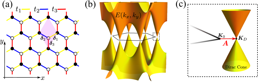
Figure 1: (Color online) (a) Honeycomb lattice and hoppings. The primitive cell, in light purple, contains a pair of Carbon atoms. (b) Dispersion relation $E(\bm{k})$ of the anisotropic honeycomb lattice and its hexagonal first Brillouin zone. (c) A zoom of the Dirac cone region shows that the Dirac point $\bm{K}_{D}$ is not located at the corner $\bm{K}_{0}$ of the hexagonal Brillouin zone. The anisotropy-induced Dirac point shift is given by the vector $\bm{A}$.

This paper is organized as follows. In Sec. II, we derive the effective Dirac Hamiltonian for a honeycomb lattice with weak anisotropy in the hopping parameters. For this purpose, we start from nearest-neighbor tight-binding model and carry out an expansion around the real Dirac point. The obtained low-energy Hamiltonian is used in Sec. III to discuss the optical properties of anisotropic honeycomb lattices, which are assumed by having linear response to an external oscillating field. In Sec. IV, our findings are particularized to the case of graphene under a nonmechanical deformation, which can not represented by means of the strain tensor. Finally, in Sec. V, our conclusions are given.

II Generalized honeycomb lattice

We are interested in the low-energy Hamiltonian, i.e. the effective Dirac Hamiltonian, of a honeycomb lattice with anisotropy in the nearest-neighbor hopping parameters. As unstrained graphene, our lattice consists of a triangular Bravais lattice with a pair of Carbon atoms (open and filled circles in Fig. 1 (a)) located in its primitive cell. However, we consider that the hoppings between nearest sites are dependent on the direction and, in general, are characterized by three hopping parameters $t_{1}$, $t_{2}$ and $t_{3}$ (see Fig. 1 (a)). Within this nearest-neighbor tight-binding model, one can demonstrate that the Hamiltonian in momentum space can be represented by a ($2\times 2$) matrix of the formKatsnelson (2012)

$$H=-\sum_{n=1}^{3}t_{n}\begin{pmatrix}0&e^{-i\bm{k}\cdot\bm{\delta}_{n}}\\ e^{i\bm{k}\cdot\bm{\delta}_{n}}&0\end{pmatrix},$$ (1)

where $\bm{\delta}_{1},\bm{\delta}_{2},\bm{\delta}_{3}$ are the nearest-neighbor vectors. Hereafter, we define the the nearest-neighbor vectors as

$$\bm{\delta}_{1}=\frac{a}{2}(\sqrt{3},1),\ \ \bm{\delta}_{2}=\frac{a}{2}(-\sqrt{3},1),\ \ \bm{\delta}_{3}=a(0,-1),$$ (2)

i.e., we choose the coordinate system $xy$ in a way that the $x$ axis is along the zigzag direction of the honeycomb lattice (see Fig. 1 (a)). We denote the system $xy$ as the crystalline coordinate system.

From Eq. (1) follows that the dispersion relation is given by two bands:

$$E(\bm{k})=\pm|t_{1}e^{i\bm{k}\cdot\bm{\delta}_{1}}+t_{2}e^{i\bm{k}\cdot\bm{\delta}_{2}}+t_{3}e^{i\bm{k}\cdot\bm{\delta}_{3}}|,$$ (3)

As is well documented, for the isotropic case $t_{1,2,3}=t_{0}$, the Dirac points $\bm{K}_{D}$, which are determined by condition $E(\bm{K}_{D})=0$, coincide with the corners of the first Brillouin zone. Then, to obtain the Dirac Hamiltonian in this case, one can simply expand the Hamiltonian (1) around a corner, e.g., $\bm{K}_{0}=(\frac{4\pi}{3\sqrt{3}a},0)$. However, for the considered anisotropic case, the Dirac points do not coincide with the corners of the first Brillouin zone (as illustrated in Fig. 1 (b,c)).Pereira et al. (2009); Li et al. (2010) In consequence, to derive the Dirac Hamiltonian, one can no longer expand the Hamiltonian (1) around $\bm{K}_{0}$. As recently demonstrated, such expansion around $\bm{K}_{0}$ yields an inappropriate Hamiltonian.Oliva-Leyva and Naumis (2015b) The appropriate procedure is to find the position of the Dirac points and carry out the expansion around them.Oliva-Leyva and Naumis (2015b); Volovik and Zubkov (2014, 2015) Note that when the hopping anisotropy increases, a gap can appear while the Dirac points disappear. Such effects are characterized by the Hasegawa triangular inequalities.Hasegawa et al. (2006)

II.1 Effective Dirac Hamiltonian

Now let us study the effect of a weak anisotropy given by a small perturbation of the hopping parameters. The perturbed hoppings are given by

$$t_{n}=t_{0}(1+\Delta_{n}),$$ (4)

on the low-energy description. As expressed above, to derive the proper effective Dirac Hamiltonian it is essential to find the position of the Dirac points.Oliva-Leyva and Naumis (2015b) In Appendix A we show that from the condition $E(\bm{K}_{D})=0$, up to first order in the parameters $\{\Delta_{n}\}$, one can obtain that $\bm{K}_{D}$ is given by

$$\bm{K}_{D}\approx\bm{K}_{0}+\bm{A},$$ (5)

where

$$A_{x}=\frac{1}{3a}(2\Delta_{3}-\Delta_{1}-\Delta_{2}),\ \ \ \ \ A_{y}=\frac{1}{\sqrt{3}a}(\Delta_{1}-\Delta_{2}),$$ (6)

and $\bm{K}_{0}$ presents valley index $\xi=+1$. As is well known,Katsnelson (2012); Vozmediano et al. (2010) the shift $\bm{A}$ of the Dirac point plays the role of an emergent gauge field, similar to a vector potential, when the hopping parameters are position-dependent throughout the sample. Thus gauge fields couple with opposite signs to valleys with different index .Katsnelson (2012); Vozmediano et al. (2010)

Once the position of $\bm{K}_{D}$ is found, we expand the Hamiltonian (1) around the Dirac point by means of $\bm{k}=\bm{K}_{D}+\bm{q}$. Following this approach up to first order in the parameters $\{\Delta_{n}\}$, which is the leading order used throughout the rest of the paper, we derive that the effective Dirac Hamiltonian results in (see Appendix B),

$$H=\hbar v_{F}\bm{\sigma}\cdot(\bar{\bm{I}}+\bar{\bm{\Delta}})\cdot\bm{q},$$ (7)

where $v_{F}=3t_{0}a/2\hbar$ is the Fermi velocity for the unperturbed honeycomb lattice, $\bm{\sigma}=(\sigma_{x},\sigma_{y})$ are the non-diagonal Pauli matrices, $\bar{\bm{I}}$ is the $2\times 2$ identity matrix and $\bar{\bm{\Delta}}$ is the symmetric matrix

$$\bar{\bm{\Delta}}=\begin{pmatrix}\frac{1}{3}(2\Delta_{1}+2\Delta_{2}-\Delta_{3})&\frac{1}{\sqrt{3}}(\Delta_{1}-\Delta_{2})\\ \frac{1}{\sqrt{3}}(\Delta_{1}-\Delta_{2})&\Delta_{3}\end{pmatrix}.$$ (8)

Let us note some important remarks about our generalized Hamiltonian (7). First of all, when the three hopping parameters $\{t_{n}\}$ are equal to $t_{0}(1+\Delta)$, we have that $\bar{\bm{\Delta}}=\Delta\bar{\bm{I}}$. Then Eq. (7) reproduces the expected result $\hbar v_{F}(1+\Delta)\bm{\sigma}\cdot\bm{q}$, which is just a renormalization of the Fermi velocity. In general, from Eq. (7) one can recognize a generalized Fermi velocity tensor as

$$\bar{\bm{v}}=v_{F}(\bar{\bm{I}}+\bar{\bm{\Delta}}),$$ (9)

whose matrix character is due to the shape of the isoenergetic contours around $\bm{K}_{D}$, which are rotated ellipses. Only for the case that $t_{1}=t_{2}$ ($\Delta_{1}=\Delta_{2}$), the Fermi velocity tensor is diagonal with respect to the crystalline coordinate system $xy$ chosen. In this case, the principal axes of the isoenergetic ellipses are collinear with the $xy$ axes. Moreover, the general character of Eq. (7) enables to estimate the variation effects of the hopping parameters for graphene under a spatially uniform strain. For the last case, to first order in the strain tensor $\tilde{\bm{\epsilon}}$, the hopping parameters are approximated by $t_{n}\approx t_{0}(1-\beta\bm{\delta}_{n}\cdot\bar{\bm{\epsilon}}\cdot\bm{\delta}_{n}/a^{2})$, where $\beta$ is the electron Grüneisen parameter. Thus, $\Delta_{n}=-\beta\bm{\delta}_{n}\cdot\bar{\bm{\epsilon}}\cdot\bm{\delta}_{n}/a^{2}$ and as a consequence, one obtain that for uniformly strained graphene, $\bar{\bm{\Delta}}=-\beta\bar{\bm{\epsilon}}$. However, to write the effective Dirac Hamiltonian for uniformly strained graphene, it should also take into account the deformation of the lattice vectors.Oliva-Leyva and Naumis (2013)

It is important to emphasize that the expression (8) for the matrix $\bar{\bm{\Delta}}$ is referred to the crystalline coordinate system $xy$. In general, if one choose an arbitrary coordinate system $x^{\prime}y^{\prime}$, rotated at an angle $\phi$ respect to the system $xy$, then the new components of $\bar{\bm{\Delta}}$ can be found by means of the transformation rules of a second order Cartesian tensor. In other words, $\bar{\bm{\Delta}}$ is a second order Cartesian tensor, whose explicit form (8) is given with respect to the crystalline coordinate system $xy$.

III Optical conductivity

Let us now study the optical properties of those anisotropic electronic honeycomb fermionic lattices that exhibit linear response to an external electric field of frequency $w$. For this purpose, we firstly obtain the optical conductivity tensor $\bar{\sigma}_{ij}(w)$ by combining the Hamiltonian (7) and the Kubo formula. Following the representation used in Refs. [Ziegler (2006, 2007)], the optical conductivity $\sigma_{ij}(w)$ can be written as a double integral with respect to two energies $E$, $E^{\prime}$:

$$\bar{\sigma}_{ij}(w)=\frac{i}{\hbar}\int\int\text{Tr}\{j_{i}\delta(H-E^{\prime})j_{j}\delta(H-E)\}$$

$$\qquad\times\frac{1}{E-E^{\prime}+w-i\alpha}\frac{f(E)-f(E^{\prime})}{E-E^{\prime}}\text{d}E\text{d}E^{\prime},$$ (10)

where $f(E)=(1+\exp[E/(k_{B}T)])^{-1}$ is the Fermi function at temperature $T$ and $j_{l}=-ie[H,r_{l}]$ is the current operator in the $l$-direction, with $l=x,y$.

To calculate the integral (III) it is convenient to carry out the change of variables

$$\bm{q}=(\bar{\bm{I}}+\bar{\bm{\Delta}})^{-1}\cdot\bm{q}^{*}$$ (11)

In the new variables $(q_{x}^{*},q_{y}^{*})$, the Hamiltonian (7) becomes $H=\hbar v_{F}\bm{\sigma}\cdot\bm{q}^{*}$, corresponding to an unperturbed honeycomb lattice, as unstrained graphene. On the other hand, the current operator components transform as

$$j_{x} = -ie[H,r_{x}]=e\frac{\partial H}{\partial q_{x}},$$ (12)

$$= e\left(\frac{\partial H}{\partial q_{x}^{*}}\frac{\partial q_{x}^{*}}{\partial q_{x}}+\frac{\partial H}{\partial q_{y}^{*}}\frac{\partial q_{y}^{*}}{\partial q_{x}}\right),$$

$$= (1+\bar{\Delta}_{xx})j_{x}^{*}+\bar{\Delta}_{xy}j_{y}^{*},$$

and analogously

$$j_{y}=(1+\bar{\Delta}_{yy})j_{y}^{*}+\bar{\Delta}_{xy}j_{x}^{*},$$ (13)

where $j_{x}^{*}=e(\partial H/\partial q_{x}^{*})$ and $j_{y}^{*}=e(\partial H/\partial q_{y}^{*})$ are the current operator components for the case of the unperturbed honeycomb lattice.

Then, substituting Eqs. (12) and (13) into Eq. (III), we obtain

$$\bar{\sigma}_{xx}(w) \simeq (1+2\bar{\Delta}_{xx})J\sigma_{0}(w),$$ (14)

$$\bar{\sigma}_{yy}(w) \simeq (1+2\bar{\Delta}_{yy})J\sigma_{0}(w),$$ (15)

$$\bar{\sigma}_{xy}(w) = \bar{\sigma}_{yx}(w)\simeq 2\bar{\Delta}_{xy}J\sigma_{0}(w),$$ (16)

where $J$ is the Jacobian determinant of the transformation (11) and $\sigma_{0}(w)$ is the optical conductivity of the unperturbed honeycomb lattice. Note that as an explicit expression for $\sigma_{0}(w)$ one can use the reported optical conductivity of unstrained graphene.Ziegler (2007); Gusynin et al. (2007); Stauber et al. (2008)

Finally, from Eqs. (14)–(16) it follows that the optical conductivity tensor for the anisotropic honeycomb lattice results in,

$$\bar{\bm{\sigma}}(w)\simeq\sigma_{0}(w)(\bar{\bm{I}}+2\bar{\bm{\Delta}}-\text{Tr}(\bar{\bm{\Delta}})\bar{\bm{I}}).$$ (17)

In other words, a Dirac system described by the generalized Hamiltonian (7) presents an anisotropic optical response given by Eq. (17), independently of the expression of matrix $\bar{\bm{\Delta}}$. Now substituting Eq. (8) into Eq. (17) we obtain the explicit form of the optical conductivity tensor for the anisotropic honeycomb lattice, respect to the crystalline coordinate system $xy$.

III.1 Dichroism and Transmittance

The anisotropy of the optical absorption yields two effects: dichroism and modulation of the transmittance as a function of the polarization direction. To examine such effects, let us consider normal incidence of linearly polarized light between two dielectric media separated by our anisotropic honeycomb lattice, as illustrated in Fig. 2(a). From the boundary conditions for the electromagnetic field on the interface between both media, one can obtain that the electric fields of the incident and transmitted waves, $\bm{E}_{i}$ and $\bm{E}_{t}$ respectively, are related byOliva-Leyva and Naumis (2015a)

$$\bm{E}_{i}=\frac{1}{2}\sqrt{\frac{\mu_{1}}{\epsilon_{1}}}\left(\left(\sqrt{\frac{\epsilon_{1}}{\mu_{1}}}+\sqrt{\frac{\epsilon_{2}}{\mu_{2}}}\right)\bar{\bm{I}}+\bar{\bm{\sigma}}\right)\cdot\bm{E}_{t},$$ (18)

where $\epsilon_{1,2}$ are the electrical permittivities and $\mu_{1,2}$, the magnetic permeabilities. Note that, in general, the anisotropy of the conductivity $\bar{\bm{\sigma}}$ produces that $\bm{E}_{i}$ and $\bm{E}_{t}$ are not collinear (see Fig. 2(b)). Analogously, the magnetic fields, $\bm{H}_{i}$ and $\bm{H}_{t}$, fulfill the same relation.

Now from Eq. (18) the calculation of the transmittance is straightforward:Oliva-Leyva and Naumis (2015a)

$$T(\theta_{i}) = \frac{|\bm{E}_{t}\times\bm{H}_{t}|}{|\bm{E}_{i}\times\bm{H}_{i}|}=\frac{\sqrt{\epsilon_{2}/\mu_{2}}|\bm{E}_{t}|^{2}}{\sqrt{\epsilon_{1}/\mu_{1}}|\bm{E}_{i}|^{2}},$$ (19)

$$\approx T_{0}\left(1-\frac{2\sqrt{\mu_{1}\mu_{2}}}{\sqrt{\epsilon_{1}\mu_{2}}+\sqrt{\epsilon_{2}\mu_{1}}}\bm{e}_{i}^{\intercal}\cdot\mbox{Re}\bar{\bm{\sigma}}\cdot\bm{e}_{i}\right),$$

where $T_{0}$ is the transmittance for normal incidence between two media in absence of the anisotropic honeycomb lattice as interface and $\bm{e}_{i}^{\intercal}=(\cos\theta_{i},\sin\theta_{i})$, with $\theta_{i}$ being the incident polarization angle $\theta_{i}$.

To illustrate even more clearly the dichroism and the modulation of $T(\theta_{i})$ induced by the anisotropic honeycomb lattice, it is convenient to consider that the chemical potential equals zero for the lattice. In consequence, for the domain of infrared and visible frequencies, in Eq. (17) $\sigma_{0}(w)$ can be replaced by the universal and frequency-independent value $e^{2}/(4\hbar)$.Stauber et al. (2008); Nair et al. (2008) Additionally, if both media are vacuum, then from Eqs.(17)-(19) we obtain that

$$\theta_{t}-\theta_{i} \approx \frac{\pi\alpha}{2}A\sin(2\theta_{i}-\theta_{0}),\ \ \ \text{(in radians)},$$ (20)

$$T(\theta_{i}) \approx 1-\pi\alpha\bigl{(}1+A\cos(2\theta_{i}-\theta_{0})),$$ (21)

where

$$A=\sqrt{(\bar{\Delta}_{xx}-\bar{\Delta}_{yy})^{2}+4\bar{\Delta}_{xy}^{2}}=\sqrt{(\mbox{Tr}\bar{\bm{\Delta}})^{2}-4\mbox{Det}\bar{\bm{\Delta}}},$$ (22)

$\sin\theta_{0}=2\bar{\Delta}_{xy}/A$ ($\cos\theta_{0}=(\bar{\Delta}_{xx}-\bar{\Delta}_{yy})/A$) and $\alpha$ is the fine-structure constant.

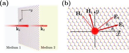
Figure 2: (Color online) (a) Scattering problem for normal incidence between two media with the anisotropic honeycomb lattice separating them. The $z$ direction is chosen along the propagation of the electromagnetic wave. $\bm{k}_{i}$ and $\bm{k}_{t}$ represent the wave vectors of the incident and transmitted waves, respectively. (b) Schematic representation of the dichroism induced by the anisotropic absorption of the honeycomb lattice. The electromagnetic fields lie in the lattice plane.

It is immediate to verify that, for $\bar{\bm{\Delta}}=0$, the dichroism disappears and $T(\theta_{i})$ reduces to $1-\pi\alpha$ $(\approx 97.7\%)$, which is the transmittance of unstrained graphene.Nair et al. (2008) Expressions (20) and (21) clearly show $\pi$-periodic modulations of the dichroism and transmittance respect to the incident polarization angle $\theta_{i}$, which is due to the physical equivalence between $\theta_{i}$ and $\theta_{i}+\pi$, for normal incidence of linearly polarized light. From Eq. (20) follows that the principal directions of $\bar{\bm{\Delta}}$ can be determined by monitoring the polarization angles $\theta_{i}$ for which the incident and transmitted polarizations coincide. At the same time, Eq. (21) shows that the principal directions of $\bar{\bm{\Delta}}$ can be determined by measuring the polarization angles $\theta_{i}$ for which the transmittance takes its minimum or maximum values. Also, it is important to note that while the phase $\theta_{0}$ of both modulations is dependent on the coordinate system orientation, the amplitude $A$ is independent on any orientation of the coordinate system, as physically expected, because $A$ is given as a function of the invariants $\mbox{Tr}\bar{\bm{\Delta}}$ and $\mbox{Det}\bar{\bm{\Delta}}$.

So far, our discussion on dichroism and transmittance is general for an anisotropic Dirac system described by Eq. (7). By substituting Eq. (8) into Eqs. (20,21), one obtains the explicit form of such effects for the anisotropic honeycomb lattice with respect to the crystalline coordinate system $xy$.

IV Application

As an application of the previous results, we consider a deformation of graphene lattice, as illustrated in Fig. 3(a). Here the primitive vectors $\bm{a}_{1}$ and $\bm{a}_{2}$ remain undeformed, while the atom of basis, denoted by an open circle, is displaced a vector $\bm{u}$ in an arbitrary direction. This deformation of graphene lattice is basically a displacement, given by $\bm{u}$, of the open-circles sublattice respect to the filled-circles sublattice. A possible scenario for such deformation could occur in graphene grown on substrate with an appropriate combination of lattice mismatch between the two crystals.Ni et al. (2014); Lee et al. (2015)

The new nearest-neighbor vectors $\bm{\delta}_{n}^{\prime}$ are related to the unstrained nearest-neighbor vectors $\bm{\delta}_{n}$ by means of $\bm{\delta}_{n}^{\prime}=\bm{\delta}_{n}-\bm{u}$. However, it is worth mentioning that the reciprocal lattice of our modified graphene lattice remains undeformed because the direct lattice, determined by $\bm{a}_{1}$ and $\bm{a}_{2}$, is undistorted. The last is a notable difference with the case of strained graphene by means of mechanical stress, for which the lattice vectors are deformed.

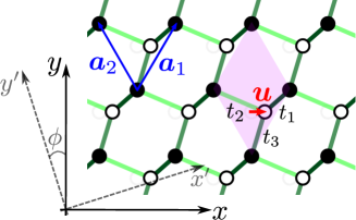
Figure 3: (Color online) Scheme of the modified graphene lattice. The red arrow represents the displacement $\bm{u}$ of the open-circles sublattice.

As in Sec. II, if we begin from a nearest-neighbor approach, it is easy to demonstrate that the dispersion relation for this modified graphene lattice reads

$$E(\bm{k}) = \pm|t_{1}e^{i\bm{k}\cdot(\bm{\delta}_{1}-\bm{u})}+t_{2}e^{i\bm{k}\cdot(\bm{\delta}_{2}-\bm{u})}+t_{3}e^{i\bm{k}\cdot(\bm{\delta}_{3}-\bm{u})}|,$$ (23)

$$= \pm|t_{1}e^{i\bm{k}\cdot\bm{\delta}_{1}}+t_{2}e^{i\bm{k}\cdot\bm{\delta}_{2}}+t_{3}e^{i\bm{k}\cdot\bm{\delta}_{3}}|,$$

where we characterize the variation of the hopping parameters in the usual form: $t_{n}=t_{0}\exp[-\beta(|\bm{\delta}_{n}^{\prime}|/a-1)]$.Pereira et al. (2009) Note that Eq. (23) coincides with Eq. (3), so the modified graphene lattice can be considered as a particular case of the generalized honeycomb lattice examined in Sec. II. Therefore, now we can particularize all general previous results for the modified graphene lattice.

Effective Dirac Hamiltonian: Writing the variation of the hopping parameters to first order in $\bm{u}$, one get

$$t_{n} = t_{0}\exp[-\beta(|\bm{\delta}_{n}-\bm{u}|/a-1)],$$ (24)

$$\approx t_{0}(1+\beta\bm{\delta}_{n}\cdot\bm{u}/a^{2}),$$

thus, for this case one can identify from Eq.(4) that $\Delta_{n}=\beta\bm{\delta}_{n}\cdot\bm{u}/a^{2}$. Consequently, from Eqs.(7) and (8), the effective Dirac Hamiltonian of the modified graphene lattice results in,

$$H=\hbar v_{F}\bm{\sigma}\cdot(\bar{\bm{I}}+\bar{\bm{\Delta}}^{u})\cdot\bm{q},$$ (25)

where the matrix $\bar{\bm{\Delta}}_{u}$ dependents on the components of the vector $\bm{u}$ as

$$\bar{\bm{\Delta}}^{u}=\frac{\beta}{a}\begin{pmatrix}u_{y}&u_{x}\\ u_{x}&-u_{y}\end{pmatrix}.$$ (26)

It is immediate to verify that for $\bm{u}=0$ one recover the case of unstrained graphene. Note that $\mbox{Tr}\bar{\bm{\Delta}}^{u}=0$, which is because the studied deformation does not vary the area of graphene sample. This fact is analogous to having a pure shear strain.

The form (26) of the tensor $\bar{\bm{\Delta}}^{u}$ is referred to the crystalline coordinate system $xy$. Now let us give its general expression respect to an arbitrary coordinate system $x^{\prime}y^{\prime}$, which is inclined to $xy$ at an angle $\phi$. Using the transformation rules of a second order Cartesian tensor we find

$$\bar{\Delta}^{u}_{x^{\prime}x^{\prime}} = -\bar{\Delta}^{u}_{y^{\prime}y^{\prime}}=\frac{\beta}{a}(u_{y^{\prime}}\cos 3\phi+u_{x^{\prime}}\sin 3\phi),$$ (27)

$$\bar{\Delta}^{u}_{x^{\prime}y^{\prime}} = \bar{\Delta}^{u}_{y^{\prime}x^{\prime}}=\frac{\beta}{a}(-u_{y^{\prime}}\sin 3\phi+u_{x^{\prime}}\cos 3\phi),$$ (28)

where $u_{x^{\prime}}$ and $u_{y^{\prime}}$ are the components of the vector $\bm{u}$ respect to the system $x^{\prime}y^{\prime}$. These expressions for the tensor $\bar{\bm{\Delta}}^{u}(\phi)$ exhibit a clear periodicity of $2\pi/3$ in $\phi$, which reflects the trigonal symmetry of the underlying honeycomb lattice.

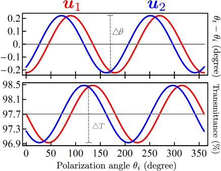
Figure 4: (Color online) Rotation of the transmitted field (top panel) and transmittance (bottom panel) as a function of the incident polarization angle for two different deformations. The red curves correspond to the displacement $\bm{u}_{1}/a=(0.05,0)$, while the blue curves correspond to the displacement $\bm{u}_{2}/a=(0.04,0.03)$.

Optical properties: From Eqs. (17) and (26), the optical conductivity for the modified graphene lattice immediately follows as

$$\bar{\bm{\sigma}}^{u}(w) = \sigma_{0}(w)(\bar{\bm{I}}+2\bar{\bm{\Delta}}^{u}),$$ (29)

$$= \sigma_{0}(w)\begin{pmatrix}1+2\beta u_{y}/a&2\beta u_{x}/a\\ 2\beta u_{x}/a&1-2\beta u_{y}/a\end{pmatrix},$$

with respect to the crystalline coordinate system $xy$. At the same time, from Eqs. (20) and (21) one obtains that, for normal incidence of linearly polarized light, the dichroism and the transmittance are characterized by

$$\theta_{t}-\theta_{i} \approx \frac{\pi\alpha\beta}{a}(u_{y}\sin 2\theta_{i}-u_{x}\cos 2\theta_{i}),$$ (30)

$$T(\theta_{i}) \approx 1-\pi\alpha-\frac{2\pi\alpha\beta}{a}(u_{y}\cos 2\theta_{i}+u_{x}\sin 2\theta_{i}),$$ (31)

where the incident polarization angle $\theta_{i}$ is measured respect to the $x$ axis of the crystalline coordinate system.

In Fig. 4, we display the evaluated expressions (30) and (31) for two different displacements, $\bm{u}_{1}/a=(0.05,0)$ and $\bm{u}_{2}/a=(0.04,0.03)$. Such deformations present the same modulation amplitude either for the rotation of the transmitted field (dichroism) as for the transmittance. The reason is simple. From (31) it follows that the transmittance modulation amplitude $\triangle T$ is determined by the module of the vector $\bm{u}$: $\triangle T=2\pi\alpha\beta|\bm{u}|/a$. Note that $|\bm{u}_{1}|=|\bm{u}_{2}|$, therefore, $\triangle T_{1}$= $\triangle T_{2}$. The analogous argument is valid for the modulation amplitude of the rotation of the transmitted field: $\triangle\phi=\pi\alpha\beta|\bm{u}|/a$.

Nowadays, measurements of transmittance can be used to characterize the deformation state in graphene sample.Ni et al. (2014); Oliva-Leyva and Naumis (2015a)

To end, let us point out how Eq. (31) serves to characterize the strain state of our modified graphene lattice by means of two measurements of transmittance. Measuring the transmittance at $\theta_{i}=0$ and $\theta_{i}=\pi/4$, from Eq. (31) one obtain that

$$u_{x} = \frac{a}{2\pi\alpha\beta}(1-\pi\alpha-T(\pi/4)),$$ (32)

$$u_{y} = \frac{a}{2\pi\alpha\beta}(1-\pi\alpha-T(0)),$$ (33)

and of this manner, the strain state can be determined.

V Conclusion

In summary, starting from a nearest-neighbor tight-binding model we derived the effective Dirac Hamiltonian of an anisotropic honeycomb lattice, beyond strained normal graphene. This general Hamiltonian results in a useful tool for studying the anisotropic dynamics of Dirac quasiparticles in artificial graphene. Moreover, it is an excellent starting point for obtaining the effective Dirac Hamiltonian in the case of position-dependent anisotropy of the honeycomb lattice.Oliva-Leyva and Naumis (2015b) We also obtained the optical conductivity tensor of the anisotropic honeycomb lattice and showed how such anisotropic optical absorption produces a modulation of the transmittance and of the dichroism as a function of the incident polarization angle. Our findings could provide a platform to characterize the anisotropy in electric artificial graphene by means of optical measurements. At the same time, they could be used for tailoring the optical properties of electric artificial graphene.

Appendix A

Here we provide the derivation of the expressions (6) for the shift vector $\bm{A}$ of the Dirac point $\bm{K}_{D}$.

The condition $E(\bm{K}_{D})=0$, which defines the Dirac points $\bm{K}_{D}$, can be equivalently rewritten as

$$\sum_{n=1}^{3}t_{n}e^{i\bm{K}_{D}\cdot\bm{\delta}_{n}}=0.$$ (34)

In the isotropic case, $t_{n}=t_{0}$, the Dirac points coincide with the corners of the first Brillouin zone, in particular, $\bm{K}_{D}=\bm{K}_{0}=(\frac{4\pi}{3\sqrt{3}a},0)$, with $\bm{K}_{0}$ being a corner with valley index $+1$. For the anisotropic case, $t_{n}=t_{0}(1+\Delta_{n})$, the Dirac points do not coincide with the corners of the first Brillouin zone, in particular, $\bm{K}_{D}\neq\bm{K}_{0}$. Then, one can propose the position of $\bm{K}_{D}$ in the form

$$\bm{K}_{D}=\bm{K}_{0}+\bm{A}+\mathcal{O}(\Delta_{n}^{2}),$$ (35)

where the unknown shift $\bm{A}$ will be looked for as a lineal combination on the parameters $\{\Delta_{n}\}$. Now, substituting Eq. (35) into Eq. (34) results

$$\sum_{n=1}^{3}t_{0}(1+\Delta_{n})e^{i(\bm{K}_{0}+\bm{A}+\mathcal{O}(\Delta_{n}^{2}))\cdot\bm{\delta}_{n}} = 0,$$

$$\sum_{n=1}^{3}(1+\Delta_{n}+i\bm{A}\cdot\bm{\delta}_{n}+\mathcal{O}(\Delta_{n}^{2}))e^{i\bm{K}_{0}\cdot\bm{\delta}_{n}} = 0,$$

$$-3aA_{x}-\Delta_{1}-\Delta_{2}+2\Delta{3}\ \ \ \ \ \ \ \ \ \ \ \ \ \ \ \ \$$

$$+i(-3aA_{y}+\sqrt{3}\Delta_{1}-\sqrt{3}\Delta_{2})+\mathcal{O}(\Delta_{n}^{2}) = 0.$$ (36)

Thus, one obtain that the shift $\bm{A}$ is given by

$$A_{x}=\frac{1}{3a}(2\Delta_{3}-\Delta_{1}-\Delta_{2}),\ \ \ \ \ A_{y}=\frac{1}{\sqrt{3}a}(\Delta_{1}-\Delta_{2}),$$ (37)

which is our Eq. (6). Following a similar calculation, the Dirac point shift respect to the corner $\bm{K}_{0}^{{}^{\prime}}=(-\frac{4\pi}{3\sqrt{3}a},0)$, with valley index $-1$, results in $-\bm{A}$.

Appendix B

In this section, we present the details of the calculations to derive the effective Hamiltonian around $\bm{K}_{D}=\bm{K}_{0}+\bm{A}$. Also, these calculations can be taken as an alternative proof of Eq. (6), as pointed out below.

Considering momenta close to the Dirac point $\bm{K}_{D}$ , i.e. $\bm{k}=\bm{K}_{D}+\bm{q}$, and expanding to first order in $\bm{q}$ and $\{\Delta_{n}\}$, Hamiltonian (1) transforms as

$$H= - \sum_{n=1}^{3}t_{n}\begin{pmatrix}0&e^{-i(\bm{K}_{0}+\bm{A}+\bm{q})\cdot\bm{\delta}_{n}}\\ e^{i(\bm{K}_{0}+\bm{A}+\bm{q})\cdot\bm{\delta}_{n}}&0\end{pmatrix},$$

$$= - \sum_{n=1}^{3}t_{0}(1+\Delta_{n})\begin{pmatrix}0&e^{-i\bm{K}_{0}\cdot\bm{\delta}_{n}}\\ e^{i\bm{K}_{0}\cdot\bm{\delta}_{n}}&0\end{pmatrix}$$

$$\times (\bar{\bm{I}}+i\sigma_{z}\bm{A}\cdot\bm{\delta}_{n})(\bar{\bm{I}}+i\sigma_{z}\bm{q}\cdot\bm{\delta}_{n}),$$

$$= - t_{0}\sum_{n=1}^{3}(i\frac{\bm{\sigma}\cdot\bm{\delta}_{n}}{a}\sigma_{z})\Bigl{(}\bar{\bm{I}}+i\sigma_{z}\bm{q}\cdot\bm{\delta}_{n}+i\sigma_{z}\bm{A}\cdot\bm{\delta}_{n}$$ (38)

$$+ \Delta_{n}\bar{\bm{I}}-(\bm{q}\cdot\bm{\delta}_{n})(\bm{A}\cdot\bm{\delta}_{n})\bar{\bm{I}}\Bigr{)},$$

where it has been assumed that the $\bm{A}$ vector is given by Eq. (6) and $\bm{K}_{0}=(\frac{4\pi}{3\sqrt{3}a},0)$ has valley index $\xi=+1$. Collecting the contribution of each term in this expression, one obtain:

$$-t_{0}\sum_{n=1}^{3}(i\frac{\bm{\sigma}\cdot\bm{\delta}_{n}}{a}\sigma_{z})=0,$$ (39)

$$-t_{0}\sum_{n=1}^{3}(i\frac{\bm{\sigma}\cdot\bm{\delta}_{n}}{a}\sigma_{z})(i\sigma_{z}\bm{q}\cdot\bm{\delta}_{n})=\hbar v_{F}\bm{\sigma}\cdot\bm{q},$$ (40)

$$-t_{0}\sum_{n=1}^{3}(i\frac{\bm{\sigma}\cdot\bm{\delta}_{n}}{a}\sigma_{z})(i\sigma_{z}\bm{A}\cdot\bm{\delta}_{n})=\hbar v_{F}\bm{\sigma}\cdot\bm{A},$$ (41)

$$-t_{0}\sum_{n=1}^{3}(i\frac{\bm{\sigma}\cdot\bm{\delta}_{n}}{a}\sigma_{z})\Delta_{n}=-\hbar v_{F}\bm{\sigma}\cdot\bm{A},$$ (42)

$$t_{0}\sum_{n=1}^{3}(i\frac{\bm{\sigma}\cdot\bm{\delta}_{n}}{a}\sigma_{z})(\bm{q}\cdot\bm{\delta}_{n})(\bm{A}\cdot\bm{\delta}_{n})=\hbar v_{F}\bm{\sigma}\cdot\bar{\bm{\Delta}}\cdot\bm{q},$$ (43)

where the $\bar{\bm{\Delta}}$ matrix is given by Eq. (8). Then, taking into account the contribution of each term in Eq. (38), the effective Dirac Hamiltonian around $K_{D}$ has the form

$$H=\hbar v_{F}\bm{\sigma}\cdot(\bar{\bm{I}}+\bar{\bm{\Delta}})\cdot\bm{q}.$$ (44)

This result also proves that the Dirac point $\bm{K}_{D}$ is given by Eqs.(5-6). Note that in the Hamiltonian (44), all terms are $\mathcal{O}(\bm{q})$, which is a consequence of an expansion around the real Dirac point and, therefore, this proves that the expression (6) for the shift $\bm{A}$ of the Dirac point is correct.

For $\bm{K}_{0}$ with valley index $\xi=-1$, the calculation is analogous, and the effective Dirac Hamiltonian results

$$H=\hbar v_{F}\bm{\sigma}^{*}\cdot(\bar{\bm{I}}+\bar{\bm{\Delta}})\cdot\bm{q}.$$ (45)

where $\bm{\sigma}^{*}=(\sigma_{x},-\sigma_{y})$.

References

- Castro Neto et al. (2009) A. H. Castro Neto, F. Guinea, N. M. R. Peres, K. S. Novoselov, and A. K. Geim, Rev. Mod. Phys. 81, 109 (2009).
- Katsnelson et al. (2006) M. I. Katsnelson, K. S. Novoselov, and A. K. Geim, Nat. Phys. 2, 620 (2006).
- Young and Kim (2009) A. F. Young and P. Kim, Nat. Phys. 5, 222 (2009).
- Calogeracos and Dombey (1999) A. Calogeracos and N. Dombey, Contemporary Physics 40, 313 (1999).
- Lee et al. (2008) C. Lee, X. Wei, J. W. Kysar, and J. Hone, Science 321, 385 (2008).
- Castellanos-Gomez et al. (2015) A. Castellanos-Gomez, V. Singh, H. S. J. van der Zant, and G. A. Steele, Annalen der Physik 527, 27 (2015).
- Pereira and Castro Neto (2009) V. M. Pereira and A. H. Castro Neto, Phys. Rev. Lett. 103, 046801 (2009).
- Guinea (2012) F. Guinea, Solid State Communications 152, 1437 (2012).
- Wang et al. (2015) B. Wang, Y. Wang, and Y. Liu, Functional Materials Letters 08, 1530001 (2015).
- Amorim et al. (2015) B. Amorim, A. Cortijo, F. de Juan, A. G. Grushin, F. Guinea, A. Gutiérrez-Rubio, H. Ochoa, V. Parente, R. Roldán, P. San-José, J. Schiefele, M. Sturla, and M. A. H. Vozmediano, arXiv:1503.00747 (2015).
- Pereira et al. (2009) V. M. Pereira, A. H. Castro Neto, and N. M. R. Peres, Phys. Rev. B 80, 045401 (2009).
- Li et al. (2010) Y. Li, X. Jiang, Z. Liu, and Z. Liu, Nano Research 3, 545 (2010).
- Cocco et al. (2010) G. Cocco, E. Cadelano, and L. Colombo, Phys. Rev. B 81, 241412 (2010).
- Gui et al. (2015) G. Gui, D. Morgan, J. Booske, J. Zhong, and Z. Ma, Applied Physics Letters 106, 053113 (2015).
- Levy et al. (2010) N. Levy, S. A. Burke, K. L. Meaker, M. Panlasigui, A. Zettl, F. Guinea, A. H. C. Neto, and M. F. Crommie, Science 329, 544 (2010).
- Lu et al. (2012) J. Lu, A. C. Neto, and K. P. Loh, Nat Commun 3, 823 (2012).
- Suzuura and Ando (2002) H. Suzuura and T. Ando, Phys. Rev. B 65, 235412 (2002).
- Morpurgo and Guinea (2006) A. F. Morpurgo and F. Guinea, Phys. Rev. Lett. 97, 196804 (2006).
- Morozov et al. (2006) S. V. Morozov, K. S. Novoselov, M. I. Katsnelson, F. Schedin, L. A. Ponomarenko, D. Jiang, and A. K. Geim, Phys. Rev. Lett. 97, 016801 (2006).
- Guinea et al. (2010) F. Guinea, M. I. Katsnelson, and A. K. Geim, Nat Phys 6, 30 (2010).
- Sloan et al. (2013) J. V. Sloan, A. A. P. Sanjuan, Z. Wang, C. Horvath, and S. Barraza-Lopez, Phys. Rev. B 87, 155436 (2013).
- Gradinar et al. (2013) D. A. Gradinar, M. Mucha-Kruczyński, H. Schomerus, and V. I. Fal’ko, Phys. Rev. Lett. 110, 266801 (2013).
- He and He (2013) W.-Y. He and L. He, Phys. Rev. B 88, 085411 (2013).
- Carrillo-Bastos et al. (2014) R. Carrillo-Bastos, D. Faria, A. Latgé, F. Mireles, and N. Sandler, Phys. Rev. B 90, 041411 (2014).
- Qi et al. (2014) Z. Qi, A. L. Kitt, H. S. Park, V. M. Pereira, D. K. Campbell, and A. H. Castro Neto, Phys. Rev. B 90, 125419 (2014).
- Burgos et al. (2015) R. Burgos, J. Warnes, L. R. F. Lima, and C. Lewenkopf, Phys. Rev. B 91, 115403 (2015).
- Guassi et al. (2015) M. R. Guassi, G. S. Diniz, N. Sandler, and F. Qu, Phys. Rev. B 92, 075426 (2015).
- Grujić et al. (2014) M. M. Grujić, M. Z. Tadić, and F. M. Peeters, Phys. Rev. Lett. 113, 046601 (2014).
- (29) D. Midtvedt, C. H. Lewenkopf, and A. Croy, arXiv:1509.02365 .
- Rostami et al. (2015) H. Rostami, R. Roldán, E. Cappelluti, R. Asgari, and F. Guinea, Phys. Rev. B 92, 195402 (2015).
- Cortijo et al. (2015) A. Cortijo, Y. Ferreirós, K. Landsteiner, and M. A. H. Vozmediano, Phys. Rev. Lett. 115, 177202 (2015).
- Bae et al. (2013) S.-H. Bae, Y. Lee, B. K. Sharma, H.-J. Lee, J.-H. Kim, and J.-H. Ahn, Carbon 51, 236 (2013).
- Shimano et al. (2013) R. Shimano, G. Yumoto, J. Y. Yoo, R. Matsunaga, S. Tanabe, H. Hibino, T. Morimoto, and H. Aoki, Nat Commun 4, 1841 (2013).
- Dong et al. (2014) B. Dong, P. Wang, Z.-B. Liu, X.-D. Chen, W.-S. Jiang, W. Xin, F. Xing, and J.-G. Tian, Nanotechnology 25, 455707 (2014).
- Oliva-Leyva and Naumis (2013) M. Oliva-Leyva and G. G. Naumis, Phys. Rev. B 88, 085430 (2013).
- Pereira et al. (2010) V. M. Pereira, R. M. Ribeiro, N. M. R. Peres, and A. H. Castro Neto, EPL 92, 67001 (2010).
- Ni et al. (2014) G.-X. Ni, H.-Z. Yang, W. Ji, S.-J. Baeck, C.-T. Toh, J.-H. Ahn, V. M. Pereira, and B. Özyilmaz, Advanced Materials 26, 1081 (2014).
- Oliva-Leyva and Naumis (2015a) M. Oliva-Leyva and G. G. Naumis, 2D Materials 2, 025001 (2015a).
- Tarruell et al. (2012) L. Tarruell, D. Greif, T. Uehlinger, G. Jotzu, and T. Esslinger, Nature 483, 302 (2012).
- Gomes et al. (2012) K. K. Gomes, W. Mar, W. Ko, F. Guinea, and H. C. Manoharan, Nature 483, 306 (2012).
- Polini et al. (2013) M. Polini, F. Guinea, M. Lewenstein, H. C. Manoharan, and V. Pellegrini, Nat. Nano. 8, 625 (2013).
- Montambaux et al. (2009) G. Montambaux, F. Piéchon, J.-N. Fuchs, and M. O. Goerbig, Phys. Rev. B 80, 153412 (2009).
- Bellec et al. (2013) M. Bellec, U. Kuhl, G. Montambaux, and F. Mortessagne, Phys. Rev. Lett. 110, 033902 (2013).
- Feilhauer et al. (2015) J. Feilhauer, W. Apel, and L. Schweitzer, arXiv:1508.03189 (2015).
- Katsnelson (2012) M. I. Katsnelson, Graphene: Carbon in Two Dimensions (Cambridge University Press, Cambridge, UK, 2012).
- Oliva-Leyva and Naumis (2015b) M. Oliva-Leyva and G. G. Naumis, Physics Letters A 379, 2645 (2015b).
- Volovik and Zubkov (2014) G. Volovik and M. Zubkov, Annals of Physics 340, 352 (2014).
- Volovik and Zubkov (2015) G. Volovik and M. Zubkov, Annals of Physics 356, 255 (2015).
- Hasegawa et al. (2006) Y. Hasegawa, R. Konno, H. Nakano, and M. Kohmoto, Phys. Rev. B 74, 033413 (2006).
- Vozmediano et al. (2010) M. A. H. Vozmediano, M. I. Katsnelson, and F. Guinea, Physics Reports 496, 109 (2010).
- Ziegler (2006) K. Ziegler, Phys. Rev. Lett. 97, 266802 (2006).
- Ziegler (2007) K. Ziegler, Phys. Rev. B 75, 233407 (2007).
- Gusynin et al. (2007) V. P. Gusynin, S. G. Sharapov, and J. P. Carbotte, International Journal of Modern Physics B 21, 4611 (2007).
- Stauber et al. (2008) T. Stauber, N. M. R. Peres, and A. K. Geim, Phys. Rev. B 78, 085432 (2008).
- Nair et al. (2008) R. R. Nair, P. Blake, A. N. Grigorenko, K. S. Novoselov, T. J. Booth, T. Stauber, N. M. R. Peres, and A. K. Geim, Science 320, 1308 (2008).
- Lee et al. (2015) S.-M. Lee, S.-M. Kim, M. Na, H. Chang, K.-S. Kim, H. Yu, H.-J. Lee, and J.-H. Kim, Nano Research 8, 2082 (2015).