Dynamic transition in Landau-Zener-Stückelberg interferometry of dissipative systems: the case of the flux qubit

Abstract

We study Landau-Zener-Stuckelberg (LZS) interferometry in multilevel systems coupled to an Ohmic quantum bath. We consider the case of superconducting flux qubits driven by a dc+ac magnetic fields, but our results can apply to other similar systems. We find a dynamic transition manifested by a symmetry change in the structure of the LZS interference pattern, plotted as a function of ac amplitude and dc detuning. The dynamic transition is from a LZS pattern with nearly symmetric multiphoton resonances to antisymmetric multiphoton resonances at long times (above the relaxation time). We also show that the presence of a resonant mode in the quantum bath can impede the dynamic transition when the resonant frequency is of the order of the qubit gap. Our results are obtained by a numerical calculation of the finite time and the asymptotic stationary population of the qubit states, using the Floquet-Markov approach to solve a realistic model of the flux qubit considering up to 10 energy levels.

I Introduction

In recent years, the experimental realization of Landau-Zener-Stückelberg (LZS) interferometryshevchenko in several systems has emerged as a tool to study quantum coherence under strong driving. LZS interferometry is realized in two-level systems (TLS) which are driven with a time periodic force. The periodic sweeps through an avoided crossing in the energy level spectrum result in successive Landau-Zener transitions. The accumulated phase between these repeated tunneling events gives place to constructive or destructive interferences, depending on the driving amplitude and the detuning from the avoided crossing. These LZS interferences have been observed in a variety of quantum systems, such as Rydberg atoms,yoakum superconducting qubits,oliver ; izmalkov ; berns1 ; cqubits ; rudner ; valenzuela ; wilson ; wilson2 ; sun ; sun2 ; wang2010 ; graaf2013 ; shevchenko2 ultracold molecular gases,mark quantum dot devices,petta2010 ; stehlik2012 ; cao2013 ; dupont2013 ; shang2013 ; nalbach2013 ; ludwig2014 ; stace2014 ; granger2015 single spins in nitrogen vacancy centers in diamond,huang ; zhou2014 nanomechanical circuits,lahaye and ultracold atoms in accelerated optical lattices.kling Several other related experimental and theoretical works have studied LZS interferometry in systems under different shapes of periodic driving,bylander ; gustavsson ; satanin2014 ; blattmann ; xu ; silveri2015 in two coupled qubits,satanin2012 in optomechanical systems,marquardt2010 and the effect of a geometric phase.geometric Furthermore, experiments in superconducting flux qubits under strong driving have allowed to extend LZS interferometry beyond two levels.valenzuela In this later case, the multi-level structure of the flux qubit, with several different avoided crossings in the energy spectrum, exhibited a series of diamond-like interference patterns as a function of dc flux detuning and microwave amplitude.valenzuela ; wen

Driven two-level systems have been extensively studied theoretically in the past. Under strong time-periodic driving fields, phenomena such as coherent destruction of tunneling (CDT) grossmann ; kayanuma and multiphoton resonances shirley ; ashhab have been analyzed. The influence of the environment has been studied within the driven spin-boson model,grifoni-hanggi applying various techniques like the path-integral formalism,hartmann or the solution of the time dependent equations for the populations of the density matrix,grifoni-hanggi ; hartmann ; popin2l ; goorden2003 ; stace2005 ; grifonih either as an integro-differential kinetic equation,popin2l or considering for weak coupling the underlying Bloch-Redfield equations,hartmann ; goorden2003 or using the decomposition of the quantum master equation into Floquet states,grifoni-hanggi ; grifonih or performing a rotating-wave approximation.stace2005 However, the theoretical results for driven TLS in contact with a quantum bath grifoni-hanggi ; hartmann ; popin2l ; goorden2003 ; stace2005 ; grifonih present some discrepancies with the experiments of LZS interferometry, particularly in the flux qubit.oliver ; berns1 ; rudner ; valenzuela In fact, these works typically predict population inversion,hartmann ; popin2l ; goorden2003 ; stace2005 ; grifonih which has not been observed in the experiments of Ref. oliver, ; berns1, ; rudner, ; valenzuela, . In a recent work we showed,fds2 that for the case of a non-resonant detuning, population inversion arises for very long driving times and it is mediated by a slow mechanism of interactions with the bath. This long-time asymptotic regime was not reached in the experiment.

Here, we will study in full detail the LZS interference patterns of the flux qubit, by considering the dependence with dc flux detuning in addition to the dependence with microwave amplitude. To this end, we calculate numerically the finite time and the asymptotic stationary population of the qubit states using the Floquet-Markov approach,grifoni-hanggi ; fds2 solving a realistic model of the flux qubit in contact with an Ohmic quantum bath. For the time scale of the experiments we find a very good agreement with the diamond patterns of Ref.valenzuela, . For longer time scales, we find a dynamic transition within the first diamond (which corresponds to the two level regime), manifested by a symmetry change in the structure of the LZS interference pattern. We also consider the case of an structured quantum bath, which can be due to a SQUID detector with a resonant plasma frequency $\Omega_{p}$. Different types of LZS interference patterns can arise in this case, depending on the magnitude of $\Omega_{p}$.

The paper is organized as follows. In Sec.II we present the model for the flux qubit and we review the basics of LZS interferometry. In Sec. III, we show our results for the emergence of a dynamic transition in the LZS interference pattern at long times. In Sec. IV we give our conclusions and an Appendix is included to describe in detail the Floquet-Markov formalism used in this paper.

II Review of Landau-Zener-Stuckelberg interferometry of the Flux Qubit

II.1 The flux qubit

Superconducting circuits with mesoscopic Josephson junctions are used as quantum bitsrevqubits and can behave as artificial atoms.nori2011 . A well studied circuit is the flux qubit (FQ) qbit_mooij ; chiorescu ; chiorescu2 which, for millikelvin temperatures, exhibits quantized energies levels that are sensitive to an external magnetic field. The FQ consists on a superconducting ring with three Josephson junctionsqbit_mooij enclosing a magnetic flux $\Phi=f\Phi_{0}$, with $\Phi_{0}=h/2e$. The circuits that are used for the FQ have two of the junctions with the same Josephson coupling energy, $E_{J,1}=E_{J,2}=E_{J}$, and capacitance, $C_{1}=C_{2}=C$, while the third junction has smaller coupling $E_{J,3}=\alpha E_{J}$ and capacitance $C_{3}=\alpha C$, with $0.5<\alpha<1$. The junctions have gauge invariant phase differences defined as $\varphi_{1}$, $\varphi_{2}$ and $\varphi_{3}$, respectively. Typically the circuit inductance can be neglected and the phase difference of the third junction is: $\varphi_{3}=-\varphi_{1}+\varphi_{2}-2\pi f$. Therefore, the system can be described with two independent dynamical variables. A convenient choice is $\varphi_{l}=(\varphi_{1}-\varphi_{2})/2$ (longitudinal phase) $\varphi_{t}=(\varphi_{1}+\varphi_{2})/2$ (transverse phase). In terms of this variables, the hamiltonian of the FQ (in units of $E_{J}$) is:qbit_mooij

$${\cal H}_{FQ}=-\frac{\eta^{2}}{4}\left(\frac{\partial^{2}}{\partial\varphi_{t}^{2}}+\frac{1}{1+2\alpha}\frac{\partial^{2}}{\partial\varphi_{l}^{2}}\right)+V(\varphi_{l},\varphi_{t})\;,$$ (1)

with $\eta^{2}=8E_{C}/E_{J}$ and $E_{C}=e^{2}/2C$. The kinetic term of the hamiltonian corresponds to the electrostatic energy of the system and the potential term corresponds to the Josephson energy of the junctions, given by

$$V(\varphi_{l},\varphi_{t})=2+\alpha-2\cos\varphi_{t}\cos\varphi_{l}-\alpha\cos(2\pi f+2\varphi_{l})\;$$ (2)

Typical flux qubit experiments have values of $\alpha$ in the range $0.6-0.9$ and $\eta$ in the range $0.1-0.6$.chiorescu ; valenzuela In quantum computation implementations qbit_mooij ; chiorescu the FQ is operated at magnetic fields near the half-flux quantum, $f=1/2+\delta f$, with $\delta f\ll 1$. For $\alpha\geq 1/2$, the potential $V(\varphi_{l},\varphi_{t})$ has two minima at $(\varphi_{l},\varphi_{t})=(\pm\varphi^{*},0)$ separated by a maximum at $(\varphi_{l},\varphi_{t})=(0,0)$. Each minima corresponds to macroscopic persistent currents of opposite sign, and for $\delta f\gtrsim 0$ ($\delta f\lesssim 0$) a ground state $|+\rangle$ ($|-\rangle$) with positive (negative) loop current is favored.

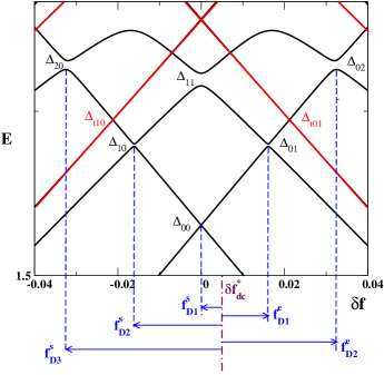
Figure 1: Lowest energy levels of the flux qubit as a function of flux detuning $\delta f$, for the qubit parameters $\eta=0.25$ and $\alpha=0.80$ considered throughout this work. Energy is measured in units of $E_{J}$ and flux in units of $\Phi_{0}$. The gaps at the avoided crossings are indicated as $\Delta_{ij}$. Black lines correspond to “longitudinal” modes and red lines to “transverse” modes (see text for description). The blue arrows at the bottom of the plot illustrate the relation between ac driving amplitudes and level crossing positions for a particular dc flux detunning $\delta f_{dc}^{*}$. The indicated values correspond to the edges of the spectroscopic diamonds of Fig.3 for the given $\delta f_{dc}^{*}$.

In Fig.1 we plot the lowest energy levels $E_{n}$ as a function of $\delta f=f-1/2$, obtained by numerical diagonalization of ${\cal H}_{FQ}$.foot1 In this case we set $\eta=0.25$ and $\alpha=0.8$, close to the experimental values employed in flux qubits experiments.qbit_mooij ; valenzuela Negative (positive) slopes in Fig.1, correspond to eigenstates with positive (negative) loop current. A gap $\Delta_{ij}$ opens at the avoided crossings of the $i$-th level of positive slope with the $j$-th level of negative slope at $\delta f=f_{ij}$. For our choice of device parameters, the avoided crossing of the two lowest levels at $\delta f=f_{00}=0$ has a gap $\Delta_{00}=3.33\times 10^{-4}$ (in units of $E_{J}$). At larger $\delta f$, we find the avoided crossing with a third level at $f_{01}=-f_{10}=0.0161$ with gap $\Delta_{01}=\Delta_{10}=2.16\times 10^{-3}$, and next the avoided crossing at $f_{02}=-f_{20}=0.0323$ with gap $\Delta_{02}=\Delta_{20}=8.26\times 10^{-3}$. (There are also energy levels that correspond to excited transverse modes,foot2 plotted with red lines in Fig.1, but they have a negligible contribution to the dynamics considered here).

The two-level regime, involving only the lowest eigenstates at $E_{0}(\delta f)$ and $E_{1}(\delta f)$, corresponds to $|\delta f|\ll f_{01}$, such that the avoided crossings with the third energy level are not reached. In this case, the hamiltonian of Eq. (1) can be reduced to a two-level systemqbit_mooij ; ferron

$${\cal H}_{TLS}=-\frac{\epsilon}{2}{\hat{\sigma}}_{z}-\frac{\Delta}{2}{\hat{\sigma}}_{x}\;,$$ (3)

in the basis defined by the persistent current states $|\pm\rangle=(|0\rangle\pm|1\rangle)/\sqrt{2}$, with $|0\rangle$ and $|1\rangle$ the ground and excited states at $\delta f=0$. The parameters of ${\cal H}_{TLS}$ are the gap $\Delta=\Delta_{00}$ and the detuning energy $\epsilon=4\pi I_{p}\delta f$. Here $I_{p}=\alpha|\langle+|\sin 2\varphi_{l}|+\rangle|=\alpha|\langle-|\sin 2\varphi_{l}|-\rangle|$ is the magnitude of the loop current, which for our case with $\alpha=0.8$ and $\eta=0.25$ is $I_{p}=0.721$ (in units of $I_{c}=2\pi E_{J}/\Phi_{0}$).

II.2 Landau-Zener-Stückelberg interferometry

Landau-Zener-Stückelberg (LZS) interferometry is performed by applying an harmonic field on top of the static field with

$$\delta f\rightarrow\delta f(t)=\delta f_{dc}+f_{ac}\sin{(\omega_{0}t)}\;.$$ (4)

If the ac driving amplitude is such that $|\delta f_{dc}\pm f_{ac}|<f_{01}$, which is fulfilled for $f_{ac}<f_{01}/2$, the quantum dynamics can be described within the two-level regime. In this case, we use $\epsilon(t)=\epsilon_{0}+A\sin(\omega_{0}t)$ in the Hamiltonian of Eq.(3), with $\epsilon_{0}=4\pi I_{p}\delta f_{dc}$ and $A=4\pi I_{p}f_{ac}$.

When $f_{ac}>|\delta f_{dc}|$ the central avoided crossing at $\delta f=0$ is reached within the range of the driving amplitude, $\delta f_{dc}\pm f_{ac}$. In this case the periodically repeated Landau-Zener transitions at $\delta f=0$ give place to LZS interference patterns as a function of $\delta f_{dc}$ and $f_{ac}$, which are characterized by multiphoton resonancesshirley and coherent destruction of tunneling,grossmann as we describe below.

There are multiphoton resonances whenshirley $E_{1}(\delta f)-E_{0}(\delta f)=n\omega_{0},$ (where $\omega_{0}$ is written in units of $E_{J}/\hbar$ and energies in units of $E_{J}$). If $\omega_{0}\gg\Delta$, these resonances are at $\epsilon_{0}=n\omega_{0}$.shevchenko ; grifoni-hanggi ; grifonih ; ashhab Calling $f_{\omega}=\omega_{0}/4\pi I_{p}$, the $n$-resonance condition can also be written as $\delta f_{dc}=nf_{\omega}$. An example of the dynamic behavior in a $n=2$ resonance is shown in Fig.2(a), calculated as described in Ref. fds, (see also the Appendix for details of the calculation). In this case the FQ is driven with frequency $\omega_{0}=0.003$ (for $E_{J}/h\sim 300$GHz it corresponds to $\omega_{0}/2\pi\sim 900$Mhz). The dc detuning is $\delta f_{dc}=0.00066$, corresponding to $\delta f_{dc}/f_{\omega}=2$ (since $f_{\omega}=\omega_{0}/4\pi I_{p}=0.00033$). The FQ is started at $t=0$ in the ground state $|\Psi(t=0)\rangle=|0\rangle$ , and the probability of having a positive loop current is calculated, $P_{+}(t)=|\langle\Psi(t)|+\rangle|^{2}$. Since for $\delta f_{dc}>0$ we have $|0\rangle\approx|+\rangle$, the initial probability is $P_{+}(t=0)\approx 1$. The red-dashed line in Fig 2(a) shows the time dependence of $P_{+}(t)$. The resonant dynamics is clearly seen: the FQ oscillates coherently between positive and negative current states. Therefore, the probability $P_{+}(t)$ oscillates between $0$ and $1$, having a time averaged value of $\overline{P_{+}}=1/2$. In contrast, Fig.2(b) shows the time dependence of $P_{+}(t)$ in an off-resonant case, for $\delta f_{dc}/f_{\omega}=4.58$. We see that for off-resonance the FQ stays in the positive loop current state, since $P_{+}(t)$ fluctuates around $P_{+}(t)\lesssim 1$.

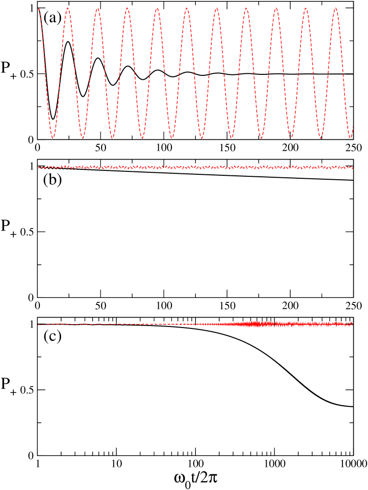
Figure 2: (Color online) Probability of a positive loop current $P_{+}$ state as a function of time, for a flux qubit driven with frequency $\omega_{0}=0.003$ (in units of $E_{J}/\hbar$). (a) $\delta f_{dc}=0.00066$ (second resonance) and $f_{ac}=0.0007$. (b) $\delta f_{dc}=0.00151$ (off resonance) and $f_{ac}=0.00245$. (c) Same as (b) but for a long time scale. Red dashed line shows the results in the non dissipative case and the black line corresponds to the dissipative case with an ohmic bath at $T=20\;mK$.

For $A\omega_{0}\gg\Delta^{2}$, it has been shown, in a rotating wave approximation, that the average probability $\overline{P_{+}}$ near a $n-$ photon resonance isshevchenko ; ashhab ; grifonih ; oliver

$$\overline{P_{+}}=1-\frac{1}{2}\frac{\Delta_{n}^{2}}{(n\omega_{0}-{\epsilon}_{0})^{2}+\Delta_{n}^{2}}\;.$$ (5)

At the resonance, $\epsilon_{0}=n\omega_{0}$, Eq.(5) gives $\overline{P_{+}}=1/2$ and away of the resonance $\overline{P_{+}}\lesssim 1$. The width of the resonance is $\delta\epsilon=|\Delta_{n}|=\Delta|J_{n}(A/\omega_{0})|=\Delta|J_{n}(f_{ac}/f_{\omega})|$, with $J_{n}(x)$ the Bessel function of the first kind. This gives a quasiperiodic dependence as a function of $f_{ac}$ for $\delta f_{dc}$ fixed near the resonance. In particular, at the zeros of $J_{n}(x)$, the resonance is destroyed, giving $\overline{P_{+}}=1$ instead of $\overline{P_{+}}=1/2$, a phenomenon known as coherent destruction of tunneling.grossmann ; kayanuma Plots of $\overline{P_{+}}$ as a function of flux detuning $\delta f_{dc}$ and ac amplitude $f_{ac}$ give the typical LZS interference patterns, which have been measured experimentally by Oliver et al in flux qubits,oliver ; berns1 ; rudner ; valenzuela and have also been observed in other systems. izmalkov ; cqubits ; wilson ; wilson2 ; sun ; sun2 ; wang2010 ; graaf2013 ; shevchenko2 ; mark ; petta2010 ; stehlik2012 ; cao2013 ; dupont2013 ; shang2013 ; nalbach2013 ; ludwig2014 ; stace2014 ; granger2015 ; huang ; zhou2014 ; lahaye ; kling

The Eq.(5) corresponds to ideally isolated flux qubits, neglecting the coupling of the qubit with the environment. The dynamics of the FQ as an open quantum system is usually characterized by the energy relaxation time $t_{r}\equiv T_{1}$ and the decoherence time $t_{dec}\equiv T_{2}$. Several phenomenological approaches have taken into account relaxation and decoherence in LZS interferometry, obtaining a broadening of the Lorentzian-shape $n-$ photon resonances of Eq.(5). For example, in Ref.shevchenko, a Bloch equation approach is used, obtaining for zero temperature:

$$\overline{P_{+}}=1-\frac{1}{2}\frac{\frac{\Gamma_{2}}{\Gamma_{1}}\Delta_{n}^{2}}{(n\omega_{0}-{\epsilon}_{0})^{2}+\frac{\Gamma_{2}}{\Gamma_{1}}\Delta_{n}^{2}+{\Gamma_{2}}^{2}}\;.$$ (6)

with $\Gamma_{1}=1/T_{1}$ and $\Gamma_{2}=1/T_{2}$. Similar results were obtained by Berns et al,berns1 considering a Pauli rate equation with an effective transition rate that adds to $\Gamma_{1}$ a driving induced rate $W$. The latter was obtained assuming that decoherence is due to a classical white noise in the magnetic flux, an approach that is valid for time scales smaller than the relaxation time and larger than the decoherence time, for $T_{1}>t\gg T_{2}$. The case of low frequency $1/\omega$ noise has been considered in a similar approach,yu2010a ; yu2010b finding a Gaussian line shape for the $n$-resonances instead of the Lorentzian line shape.

III Dynamic transition in LZS interference patterns

III.1 The driven flux qubit with an Ohmic bath

The description of the LZS interference patterns with phenomenological approaches like Eq.(6) gives a good agreement with most of the experimental results.valenzuela ; wen However, they rely on approximations valid either for large frequencies, or for low ac amplitudes, or for time scales smaller than the relaxation time. Here we will study LZS interferometry using the Floquet formalism for time-periodic Hamiltonians,shirley ; grifoni-hanggi ; grifonih ; fds which allows for an exact treatment of driving forces of arbitrary strength and frequency. The time-dependent Schrödinger equation is transformed to an equivalent eigenvalue equation for the Floquet states $|\alpha(t)\rangle$ and quasi-energies $\varepsilon_{\alpha}$, which can be solved numerically. (See the Appendix for details). To describe relaxation and decoherence processes, we consider that the qubit is weakly coupled to a bath of harmonic oscillators. The Markov approximation of the bath correlations is performed after writing the reduced density matrix $\hat{\rho}$ of the qubit in the Floquet basis, $\rho_{\alpha\beta}(t)=\langle\alpha(t)|\hat{\rho}(t)|\beta(t)\rangle$.grifoni-hanggi ; grifonih ; fds2 By following this procedure, the quantum master equation obtained for $\rho_{\alpha\beta}$ is valid for periodic driving forces of arbitrary strength. (In contrast, the standard Born-Markov approach is valid for small driving forces). The obtained Floquet-Markov quantum master equation is grifoni-hanggi ; grifonih ; fds2 :

$$\frac{d\rho_{\alpha\beta}(t)}{dt} = \sum_{\alpha^{\prime}\beta^{\prime}}\Lambda_{\alpha\beta\alpha^{\prime}\beta^{\prime}}\;\rho_{\alpha^{\prime}\beta^{\prime}}\,,$$ (7)

$$\Lambda_{\alpha\beta\alpha^{\prime}\beta^{\prime}} = -\frac{i}{\hbar}(\varepsilon_{\alpha}-\varepsilon_{\beta})\delta_{\alpha\alpha^{\prime}}\delta_{\beta\beta^{\prime}}+L_{\alpha\beta\alpha^{\prime}\beta^{\prime}}\;.$$ (8)

The coefficients ${\it L}_{\alpha\beta\alpha^{\prime}\beta^{\prime}}$ depend on the spectral density $J(\omega)$ of the bath, the temperature $T$, and on the qubit-bath coupling. Using the numerically obtained Floquet states $|\alpha(t)\rangle$, we can calculate the coefficients ${\it L}_{\alpha\beta\alpha^{\prime}\beta^{\prime}}$ , and then we compute the solution of $\rho_{\alpha\beta}(t)$ as described in the Appendix.

Here, we will consider the dynamics of a FQ coupled to a bath with an ohmic spectral densitygrifoni-hanggi ; grifonih ; fds2

$$J(\omega)=\gamma\omega e^{-\omega/\omega_{c}},$$

with $\omega_{c}$ a cutoff frequency. The Ohmic bath mimics an unstructured electromagnetic environment that in the classical limit leads to white noise. We consider $\gamma=0.001$, corresponding to weak dissipation,oliver ; valenzuela and a large cutoff $\omega_{c}=1.0E_{J}/\hbar\gg\omega_{0}$. The bath temperature is taken as $T=0.0014E_{J}/k_{B}$ ($\sim 20{\rm mK}$ for $E_{J}/h\sim 300{\rm GHz}$).

Experimentally, the probability of having a state of positive or negative persistent current in the flux qubit is measured.chiorescu ; oliver ; valenzuela The probability of a positive loop current measurement can be calculated in general asfds ; fds2

$$P_{+}(t)={\rm Tr}[\hat{\Pi}_{+}\hat{\rho}(t)]$$

with $\hat{\Pi}_{+}$ the operator that projects wave functions on the $\varphi_{l}>0$ subspace, as described in the Appendix. In Fig 2 the black lines show the population $P_{+}$ as a function of time obtained from the numerical solution of Eq.(7), taking the ground state $|0\rangle$ as initial condition, and compared with the isolated FQ (red dashed lines) discussed in the previous section. In Fig 2(a), for the $n=2$ resonance, we see that the population $P_{+}(t)$ has damped oscillations that tend to the asymptotic average value of $\overline{P_{+}}=1/2$ for large times. On the other hand, for the off-resonant case of Fig 2(b) and (c) we see that there is a clear difference between the short time behavior of $P_{+}(t)$, shown in Fig 2(b), and the large time behavior shown in Fig 2(c). Moreover, we observe that $P_{+}(t)$ tends to asymptotic values that are very different than in the isolated system. For the particular case shown in the plot, we find population inversion, i.e $P_{+}<1/2$, in the asymptotic long time limit, a phenomenon we discussed in Ref.fds2, for off-resonant cases. In the following, we will see how this change of behavior in the long time is reflected in the full LZS interference pattern as a function of $\delta f_{dc}$ and$f_{ac}$.

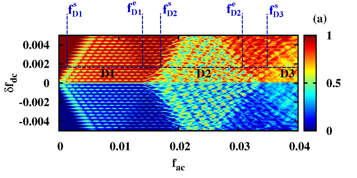
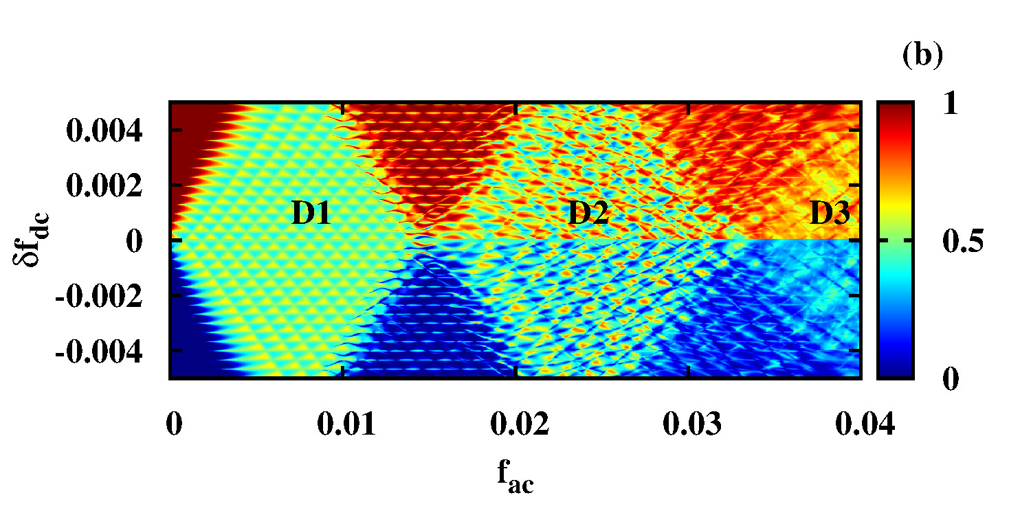
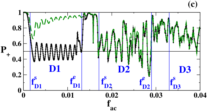
Figure 3: Landau-Zener-Stuckelberg interference patterns. Showed are intensity plots of $P_{+}$ as a function of the driving amplitude $f_{ac}$ and dc detuning $\delta f_{dc}$ for (a) $t=1000\tau$, time scale of the experiments, and (b) asymptotic regime for $t\rightarrow\infty$. In (a) we mark the ac amplitudes defined in the text that correspond to the edges of the spectroscopic diamonds for a given $\delta f_{dc}^{*}$. (c) $P_{+}$ for $\delta f_{dc}=0.00151$ as a function of the driving amplitude $f_{ac}$, at $t=1000\tau$ (blue dashed line) and asymptotic average population $\overline{P}_{+}$ (black line) . The calculations were performed for $\omega_{0}=2\pi/\tau=0.003E_{J}/\hbar$ and ohmic bath at $T=0.0014E_{J}/k_{B}\sim 20$mK. Vertical lines separate diamond regimes D1, D2, D3, described in the text.

III.2 Dynamic transition in LZS interferometry

In Figs.3(a) and 3(b) we show an intensity plot of $P_{+}$ as a function of $\delta f_{dc}$ and $f_{ac}$, calculated at a time near the experimental time scale of Refs.oliver, ; berns1, ; valenzuela, , $t_{exp}=1000\tau$, with $\tau=2\pi/\omega$ the period of the ac driving. For $f_{ac}<f_{01}/2$ we observe an LZS pattern modulated by multiphoton resonances and coherence destruction of tunneling, which can be described within a good approximation with Eq.(6). This LZS interference plot is very similar to the experimental results of Ref.oliver, ; valenzuela, . Furthermore, for higher ac amplitudes, we find a pattern of “spectroscopic diamonds”, also in good agreement with experiments.valenzuela The diamond structure obtained for high ac amplitudes can be related to the energy level spectrum of Fig.1, for a fixed dc flux detuning $f_{01}>\delta f_{dc}>0$, as follows.valenzuela ; wen The first diamond, D1, starts when the $\Delta_{00}=\Delta$ avoided crossing at $\delta f=f_{00}=0$ is reached by the amplitude of the ac drive, i.e. when $f_{00}=\delta f_{dc}\pm f_{ac}=0$. This defines an onset ac amplitude $f_{D1}^{s}=\delta f_{dc}$. The first diamond ends when the nearest second avoided crossing is reached (with gap $\Delta_{01}$) at the ac amplitude $f_{D1}^{e}=f_{01}-\delta f_{dc}$. Then the second diamond, D2, starts when the other second avoided crossing is reached, at $f_{D2}^{s}=\delta f_{dc}-f_{10}$, and it ends when the next avoided crossing is reached at $f_{D2}^{e}=f_{02}-\delta f_{dc}$. Similarly, the third diamond, D3, starts at $f_{D3}^{s}=\delta f_{dc}-f_{20}$, and so on. The analysis of the positions of the resonances as a function of $f_{ac}$ and $\delta f_{dc}$ was the route followed in Refs.valenzuela, to obtain the parameters characterizing the different avoided crossings of the flux qubit.

The FQ of Refs.oliver, ; valenzuela, have short decoherence times ($t_{dec}\sim 20{\rm ns}>\tau=\frac{2\pi}{\omega_{0}}\sim 1-10{\rm ns}$) and large relaxation times ($t_{r}\sim 100\mu{\rm s}$). The typical duration of the driving pulses in these experimental measurements ($t_{exp}\sim 3\mu{\rm s}$) is in between this two time scales, $t_{dec}<t_{exp}<t_{r}$. Due to this time scale separation, a model with classical noise,berns1 valid for $t\ll t_{r}$, can qualitatively explain the experimentally observed behavior of $P_{+}$ within the first diamond, through Eq.(6).oliver ; shevchenko Moreover, a multilevel extension of the model of Ref.berns1, can also describe the higher order diamonds (provided one gives as an input parameter the positions $f_{ij}$ and the gaps $\Delta_{ij}$ of the avoided crossings).wen

For large times $t\gg t_{r}$ one would expect naively, that after full relaxation with the environment, a blurred picture of the LZS interference pattern of Figs.3(a) with broadened resonance lobes should be observed. The asymptotic ${\overline{P}_{+}}\equiv{\lim}_{t\rightarrow\infty}\langle P_{+}(t)\rangle_{\tau}$, averaged over one period $\tau$, is shown in Fig.3(b). [ ${\overline{P}_{+}}$ can be calculated exactly after obtaining numerically the right eigenvector of $\Lambda_{\alpha\beta\alpha^{\prime}\beta^{\prime}}$ with zero eigenvalue. See the Appendix for details.] Surprisingly, we see in Fig.3(b) that the asymptotic behavior of $P_{+}$ gives a qualitatively different LZS interference pattern within the first diamond, and not a mere blurred version of Fig.3(a). In particular, a cut at constant $\delta f_{dc}$ is shown in Fig.3(c). There we see clearly that within the first diamond regime, $f_{D1}^{s}<f_{ac}<f_{D1}^{e}$, the value of $P_{+}$ at the experimental time scale is very different than the asymptotic value ${\overline{P}_{+}}$. On the other hand, beyond the first diamond, for $f_{ac}>f_{D1}^{e}$ the results of $P_{+}(t_{exp})$ and ${\overline{P}_{+}}$ are nearly coincident.

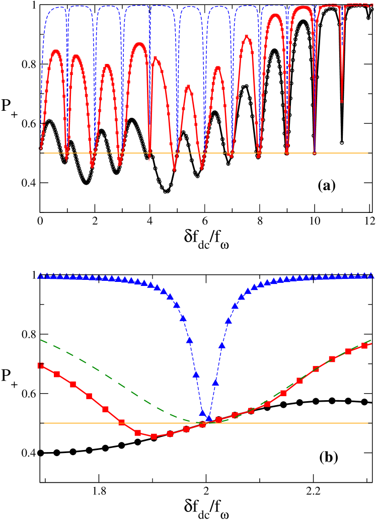
Figure 4: (color online) (a) Population $P_{+}$ as a function of the $dc$ flux detuning $\delta f_{dc}$ for the flux qubit driven with $f_{ac}=0.00245$ and $\omega_{0}=2\pi/\tau=0.003E_{J}/\hbar$, and coupled to an ohmic bath at $T=20$mK (for $E_{J}/h\approx 300{\rm GHz}$). Red line with squares: $t=1000\tau$. Black line with circles: asymptotic ($t\rightarrow\infty$) average population $\overline{P}_{+}$. Blue line with triangles: time averaged population in the isolated system. Horizontal orange line: indicates the $P_{+}=0.5$ level to help to identify when there is population inversion. The flux detuning $\delta f$ is normalized by $f_{\omega}=\omega_{0}/4\pi I_{p}$, such that the $n$-photon resonances are at $\delta f=nf_{\omega}$. (b) Enlarged view around the $n=2$ resonance. The green dashed line is a plot of the best fit with Eq.(6), while a plot of Eq.(5) (not shown) falls exactly over the blue dotted line.

In Fig.4 we show $P_{+}$ vs. $\delta f_{dc}$, for $f_{ac}=0.00245$, within the first diamond. The blue line with triangles corresponds to the solution of the isolated system, which shows dips where $P_{+}\approx 1/2$ that correspond to the $n$-photon resonances at $\delta f_{dc}/f_{\omega}=n$. The red line with squares corresponds to $P_{+}(t_{exp})$, which shows values of $P_{+}$ smaller than in the isolated case (due to effect of decoherence and relaxation) and in agreement with the experiments. The asymptotic ${\overline{P}_{+}}$ is also shown in Fig.4 (black line with circles), which is lower than $P_{+}(t_{exp})$. Fig.4(b) shows in detail the behavior near the $n=2$ resonance. The isolated case shows a dip with a Lorentzian shape accurately described by Eq.(5). The open system at the experimental time scale shows a broadened peak for $P_{+}(t_{exp})$, partially consistent with a description like Eq.(6), except that near the resonance the behavior of $P_{+}$ vs $\delta f_{dc}$ becomes antisymmetric around $\delta f_{dc}/f_{\omega}=n$. In the asymptotic steady regime, ${\overline{P}_{+}}$ vs $\delta f_{dc}$ is antisymmetric in a wide region around $\delta f_{dc}/f_{\omega}=n$, showing population inversion (${\overline{P}_{+}}<1/2$) below the resonance, for $\delta f_{dc}/f_{\omega}\lesssim n$.

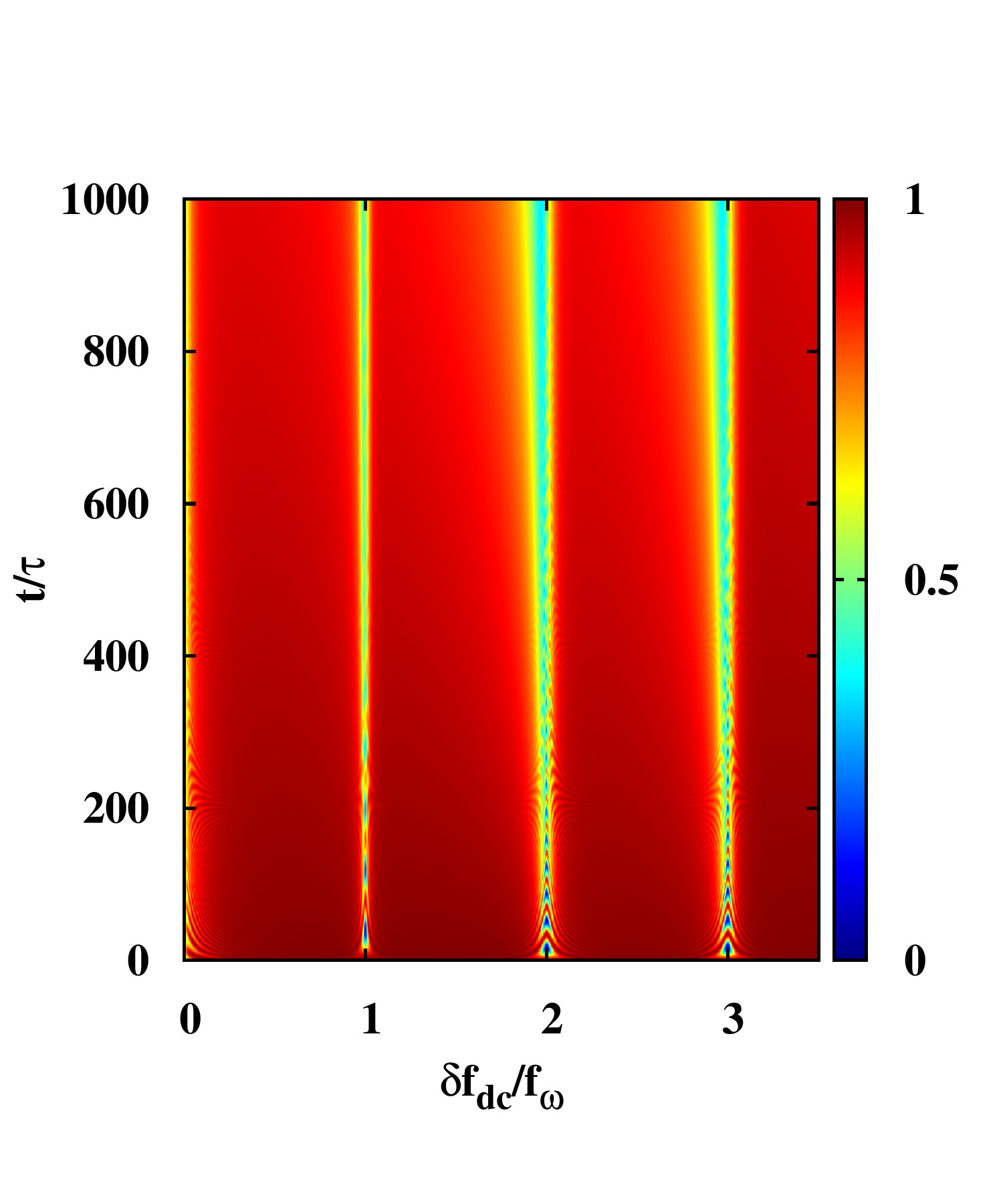
(a)  $T=1.4$ mK

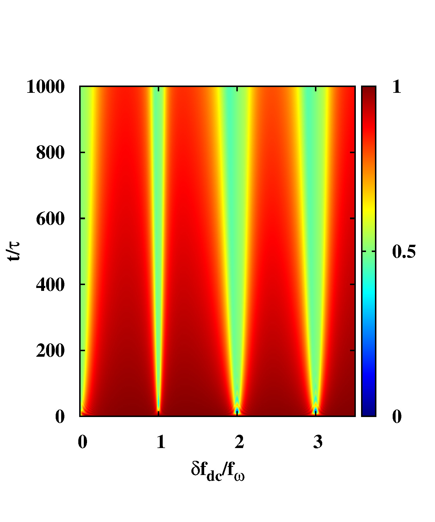
(b)  $T=20$ mK

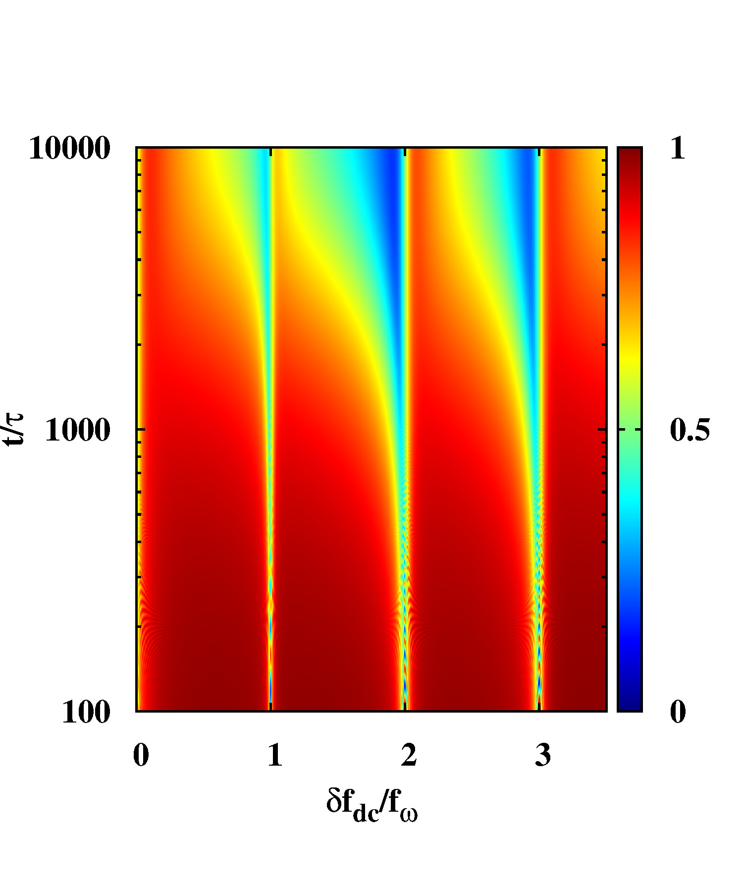
(c)  $T=1.4$ mK

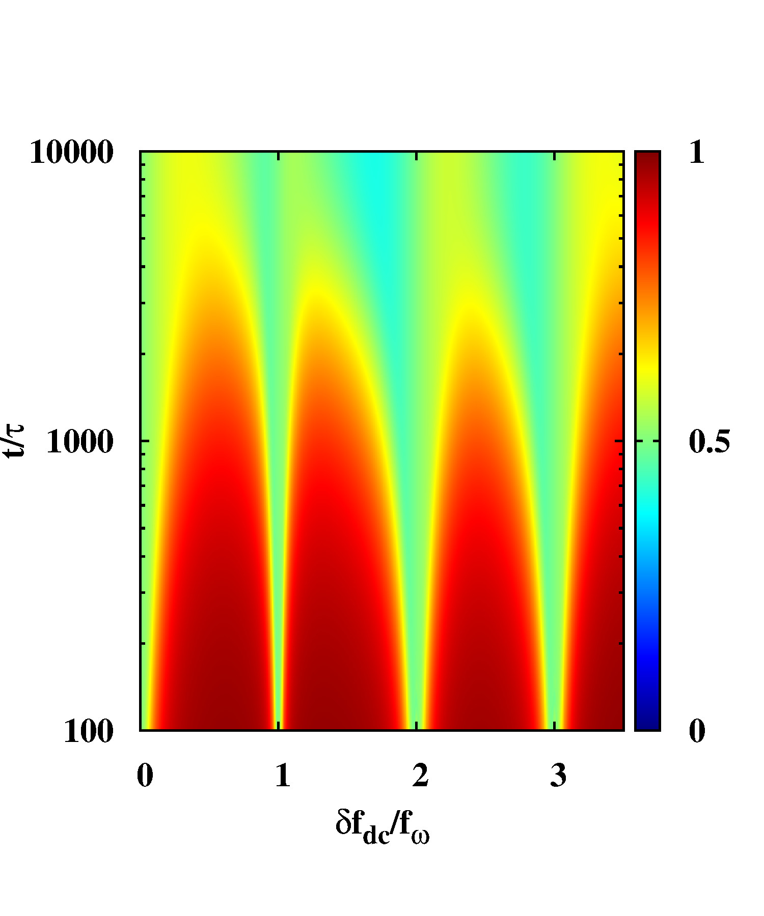
(d)  $T=20$ mK

Figure 5: (color online) Intensity plots of the population $P_{+}$ as a function of $\delta f_{dc}$ and driving time $t$ for the flux qubit driven with $f_{ac}=0.00245$ and $\omega_{0}=0.003E_{J}/\hbar$, and different temperatures. In (a) and (b) time is plotted in linear scale up to times of the order of the duration of the driving pulses in the experiments. In (c) and (d) time is plotted in logarithmic scale showing the dynamic transition to antisymmetric resonances for large times, when $t\gg t_{r}$. The flux detuning $\delta f_{dc}$ is normalized by $f_{\omega}=\omega_{0}/4\pi I_{p}$, such that the $n$-photon resonances are at $\delta f=nf_{\omega}$, and time is normalized by the driving period $\tau=2\pi/\omega_{0}$. $T$ values are given in mK, corresponding to devices with $E_{J}/h\approx 300{\rm GHz}$.

The temporal evolution from symmetric to antisymmetric resonances can be seen in detail in Fig.5, where we show an intensity plot of $P_{+}$ as a function of $\delta f_{dc}$ and the duration time $t$, for $f_{ac}=0.00245$. Two different temperatures are considered, a low temperature $T=1.4mK<\Delta$ in Figs.5(a) and (c), and $T=20mK>\Delta$ in Figs.5(b) and (d). The relaxation time $t_{r}$ for the driving amplitude considered in Fig.5 is $t_{r}\approx 1720\tau$ (as we will see in Sec.IIIC, $t_{r}$ depends on $f_{ac}$). Figs.5(a) and (b) are for duration times up to the time scale $t_{exp}\sim 1000\tau$ of the experiments, for the two different temperatures. We see that within this time scale $t_{exp}<t_{r}$, the resonances are symmetric. In Figs.5(c) and (d) the duration time is plotted in logarithmic scale and the evolution at very large times is shown. We see that at a time $t\sim t_{r}$ the resonances start to change form, becoming asymmetric in the long time limit. The asymmetry is stronger for low temperatures, in particular for $T<\Delta$ there is full inversion of population on one side of the resonances.

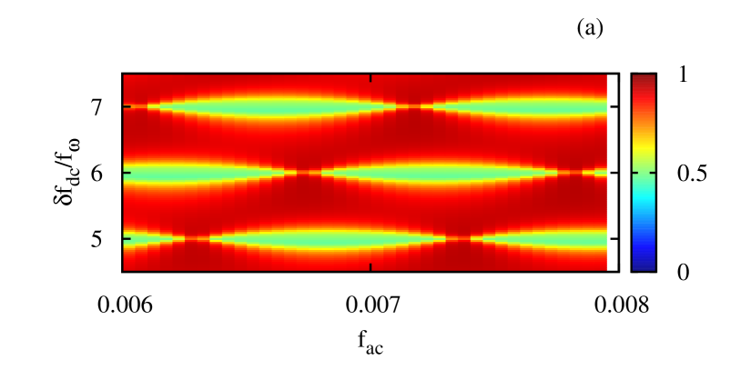
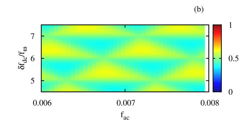
Figure 6: (Color online) Dynamic transition in the LZS interference pattern from: (a) resonance lobes for $t=1000\tau\sim t_{exp}$, to (b) triangular checkerboard pattern for asymptotic long times. Enlarged views of Fig.3(a) and (b), respectively, showing a sector of the first diamond including the $n=5,6,7$ multiphoton resonances. The flux detuning $\delta f$ is normalized by $f_{\omega}=\omega_{0}/4\pi I_{p}$, such that the $n$-photon resonances are at $\delta f=nf_{\omega}$.

Fig.5 shows that, as a function of time, there is a dynamic transition manifested by a symmetry change in the structure of the LZS interference pattern. The dynamic transition is from nearly symmetric resonances at short times ($t\ll t_{r}$) to antisymmetric resonances at long times ($t\gg t_{r}$). This is clearly illustrated in Fig.6 where an enlarged view of a part of the first diamond is shown. Fig.6(a) corresponds to $P_{+}(t_{exp})$ and shows the characteristic features observed in experiments: (i) $P_{+}\approx 1$ away from the resonances, (ii) there are resonance lobes where $P_{+}\approx 0.5$, and (iii) the $n$-resonance lobes are limited by the points where there is coherent destruction of tunneling (CDT), given by $J_{n}(f_{ac}/f_{\omega})=0$. On the other hand, in the asymptotic regime, [(Fig.6(b)], the pattern of symmetric $n$-resonance lobes is replaced by a pattern of antisymmetric resonances, which form a triangular checkerboard picture defined by triangles with $P_{+}<0.5$ and $P_{+}>0.5$ alternatively, with their vertices located at the CDT points. We name, in short, the former pattern of LZS interferometry as “symmetric resonances” (SR) and the latter as “antisymmetric resonances” (AR).

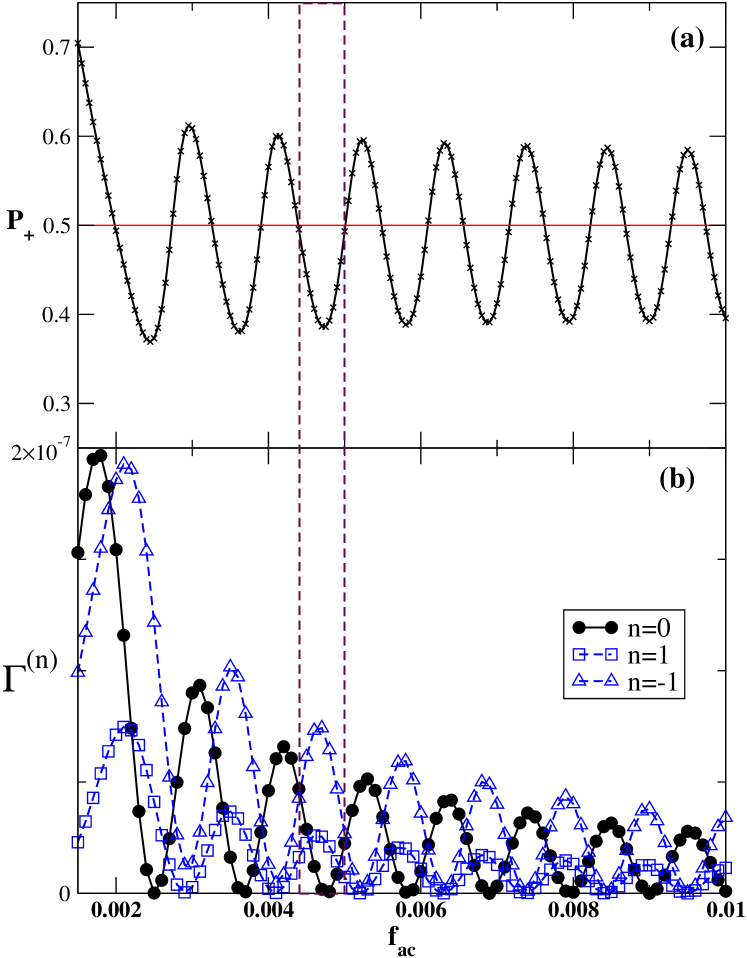
Figure 7: (a) Terms $\Gamma^{(n)}$ that contribute to the relaxation rate. as a function of the driving amplitude $f_{ac}$. The calculations were performed for $\delta f_{dc}=0.00151$, $\omega_{0}=2\pi/\tau=0.003E_{J}/\hbar$ and an ohmic bath at $T=20\rm{mK}$ (for $E_{J}/h\approx 300{\rm GHz}$). (b) Asymptotic average population $\overline{P}_{+}$ for the same case. The dashed vertical lines highlight one of the regions of $f_{ac}$ where there is population inversion.

III.3 Relaxation, decoherence and the bath-mediated population inversion mechanism

The asymptotic AR interference patterns show population inversion (PI) on one side of a multiphoton resonance, as seen in Fig.4(b) and Figs.5(c) and (d). This makes $\overline{P_{+}}$ antisymmetric around the resonance. If we fix $\delta f_{dc}$ at a value in between two resonances, the probability oscillates around $\overline{P_{+}}=1/2$ as function of $f_{ac}$, showing PI whenever a “triangle” with $\overline{P_{+}}<1/2$ is traversed. This is shown in Fig.7(a).

The underlying mechanism of this population inversion can be understood by analyzing the contribution to relaxation of virtual photon exchange processes with the bath.stace2005 ; fds2 As we show in the Appendix, within the first diamond regime, the total relaxation rate $\Gamma_{r}$ can be decomposed as

$$\Gamma_{r}=\Gamma^{(0)}+\sum_{n\not=0}\Gamma^{(n)}\;,$$

with $\Gamma^{(n)}$ the relaxation rates due to virtual $n$-photon transitions to bath oscillator states.grifonih ; stace2005 ; fds2 In Fig.7(b) we plot $\Gamma^{(n)}$ as a function of $f_{ac}$ for the same $\delta f_{dc}$ considered in Fig.7(a). We show the cases with $n=0,\pm 1$, where $\Gamma^{(0)}$ describes the relaxation without exchange of virtual photons, corresponding to the “conventional” dc relaxation mechanism, while $\Gamma^{(\pm 1)}$ correspond to the the ac contribution due to the exchange of one virtual photon with energy $\pm\hbar\omega_{0}$. We show in Fig.7 that, whenever there is population inversion, the dc relaxation terms vanish ($\Gamma^{(n=0)}\approx 0$), while the $\Gamma^{(n=-1)}$ term is the largest one. This indicates that the relevant mechanism leading to PI is a transition to a virtual level at energy $E_{0}+\hbar\omega_{0}>E_{1}$ (one photon absorption, $n=-1$), followed by a relaxation to the level $E_{1}$.stace2005 ; fds2

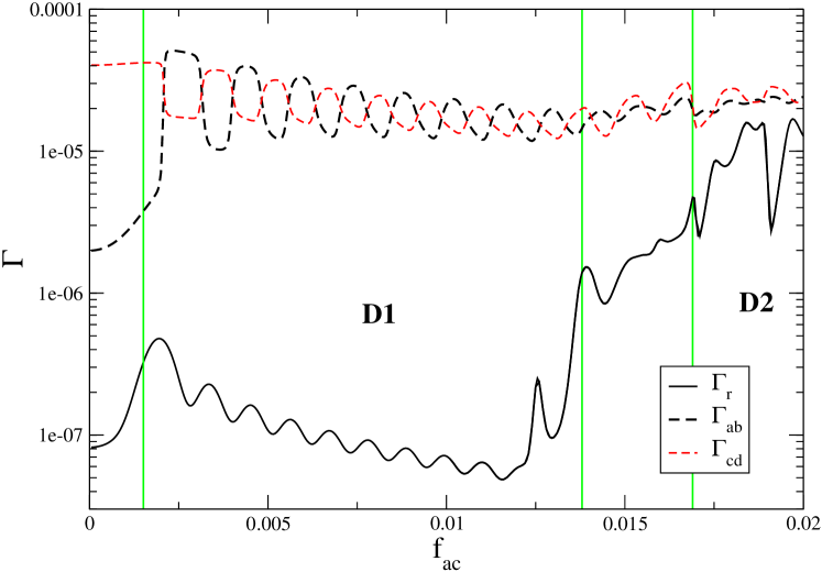
Figure 8: Relaxation rate $\Gamma_{r}$ and decoherence rates $\Gamma_{ab}$ and $\Gamma_{cd}$ as a function of the driving amplitude $f_{ac}$. The calculations were performed for $\delta f_{dc}=0.00151$, $\omega_{0}=2\pi/\tau=0.003E_{J}/\hbar$ and an ohmic bath at $T=20\rm{mK}$ (for $E_{J}/h\approx 300{\rm GHz}$). Vertical lines separate diamond regimes D1 and D2 described in the text.

To better understand why the AR patterns have not been observed yet in current experiments, we now analyze the time scales of relaxation and decoherence. To this end, we calculate numerically the full relaxation rate $\Gamma_{r}$ and the decoherence rates $\Gamma_{\alpha\beta}$, from the eigenvalues of the $\Lambda_{\alpha\beta\alpha^{\prime}\beta^{\prime}}$ matrix, as discussed in the Appendix. In Fig.8 we show the relaxation rate $\Gamma_{r}$ and two decoherence rates $\Gamma_{\alpha\beta}$, as a function of the driving amplitude $f_{ac}$ for $\delta f_{dc}=0.00151$ (away from a $n$-resonance). For $f_{ac}=0$ the relaxation rate $\Gamma_{r}$ corresponds to the $1/T_{1}$ measured experimentally, i.e., $\Gamma_{r}=1/t_{r}\rightarrow\Gamma_{1}=1/T_{1}$ when $f_{ac}\rightarrow 0$. Since to a good approximation the density matrix becomes diagonal in the Floquet basis in the asymptotic regime,grifoni-hanggi the decoherence rate $\Gamma_{ab}$ shown in Fig.8 corresponds to the decoherence between the $|a\rangle$ and the $|b\rangle$ Floquet states. When $f_{ac}\rightarrow 0$, $\Gamma_{ab}\rightarrow\Gamma_{2}=1/T_{2}$, since in this limit it corresponds to the decoherence between the two lowest energy levels. We also plot in Fig.8 the rate $\Gamma_{cd}$, which is the decoherence rate between the $|c\rangle$ and the $|d\rangle$ Floquet states. At $f_{ac}=0$ it corresponds to the decoherence between the third and the fourth energy level.

For small $f_{ac}$, below the onset of the first diamond ($f_{ac}<f_{D1}^{s}$), the relaxation and decoherence rates stay in values similar to the undriven case. However, when $f_{ac}>f_{D1}^{s}$ we see in Fig.8 that both rates depend strongly on $f_{ac}$. Above the onset of the first diamond, the overall behavior is that the decoherence rate $\Gamma_{ab}$ increases and the relaxation rate $\Gamma_{r}$ decreases as a function of $f_{ac}$. Therefore, within the first spectroscopic diamond, the difference between decoherence and relaxation is much larger than in the undriven case ($\Gamma_{ab}\gg\Gamma_{r}$). This explains the important difference between $P_{+}(t_{exp})$ and ${\overline{P}_{+}}$, within the first diamond in Fig.3, due to the large time window where AR patterns can be observed for $\Gamma_{ab}^{-1}<t_{exp}<\Gamma_{r}^{-1}$.

Beyond the first diamond, for $f_{ac}>f_{D1}^{e}$, the relaxation rate $\Gamma_{r}$ increases strongly with $f_{ac}$, becoming nearly of the same order of the decoherence rates within the second diamond and above. This behavior is a consequence of the fact that when more than two-levels are involved in the dynamics, there are several possible decay transitions between energy levels that contribute to a faster relaxation of the system. Therefore, in the second diamond and beyond decoherence and relaxation rates become comparable. For this reason, $P_{+}(t_{exp})\approx\overline{P_{+}}$ in this case, since the relaxation time is significantly reduced and thus $\Gamma_{ab}^{-1}\sim\Gamma_{r}^{-1}<t_{exp}$.

Although previous works have found PI for the asymptotic regime of two level systems,popin2l ; hartmann ; stace2005 ; yu2010a the time-dependent dynamics with different time scales has been overlooked. In fact, the relevant point from our findings is that the asymptotic regime is difficult to reach in the experiment, since PI needs long times ($t\gtrsim t_{r}\gg t_{dec}$) to emerge when mediated by the bath.

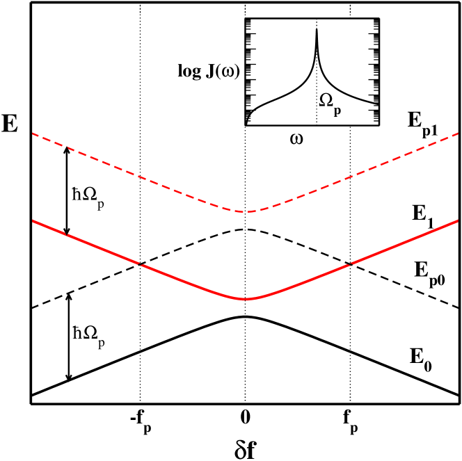
Figure 9: (Color online) Schematic plot of the two low energy levels $E_{0},E_{1}$ and the two virtual levels $E_{p0},E_{p1}$ as a function of the flux detuning $\delta f$, for the flux qubit coupled with an structured bath with a resonant mode at frequency $\Omega_{p}$. The location of the “virtual crossings” at $\pm f_{p}$ are also indicated. The inset shows a plot of the spectral density $J(\omega)$ of the structured bath.

III.4 Effect of a resonant mode in the bath

The measurement of the state of the FQ is performed with a read-out dc SQUID, which is inductively coupled to the qubit.oliver ; valenzuela ; chiorescu2 ; caspar This modifies the bath spectral density by adding a resonant mode at the plasma frequency $\Omega_{p}$ of the SQUID detector. The so-called “structured bath” spectral density is given bycaspar

$$J(\omega)=\frac{\gamma\omega\Omega_{p}^{4}}{(\Omega_{p}^{2}-\omega^{2})^{2}+(2\pi\kappa\omega\Omega_{p})^{2}},$$ (9)

with $2\pi\kappa\Omega_{p}$ the width of the resonant peak at $\omega=\Omega_{p}$ (see the inset of Fig.9 for a schematic plot of $J(\omega)$).

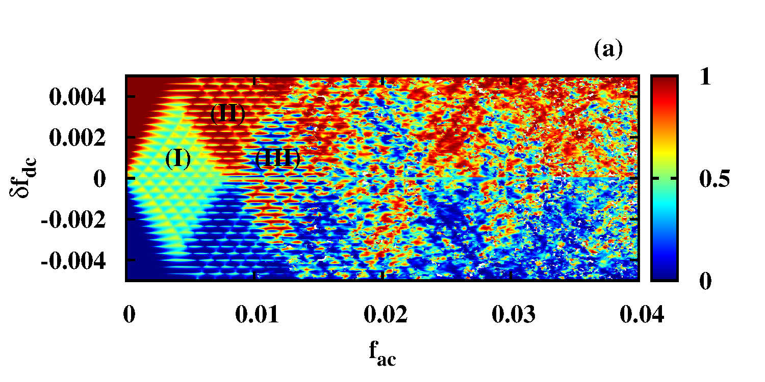
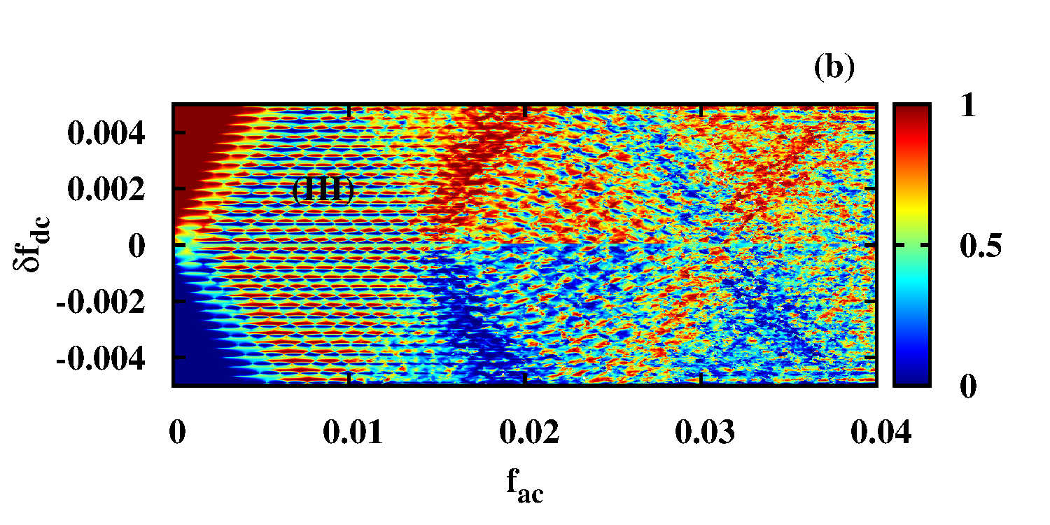
Figure 10: (Color online) Landau-Zener-Stuckelberg interference patterns for a flux qubit in contact with a structured bath. Showed are intensity plots of the asymptotic average population $\overline{P_{+}}$ as a function of the driving amplitude $f_{ac}$ and dc detuning $\delta f_{dc}$ for (a) $\Omega_{p}=0.08$ and (b) $\Omega_{p}=0.02$. We indicate in the plot the regions corresponding to the regimes (I), (II) and (III) described in the text.

Here, we study the effect of this resonant mode at $\Omega_{p}$ on LZS interferometry, in the case $\Omega_{p}>\omega_{0}$. To this end, we calculate the asymptotic ${\overline{P}_{+}}$ using the spectral density of Eq.(9), considering different values of $\Omega_{p}$, with $\kappa=0.001$ fixed.

In Fig.10 we show the intensity plots of ${\overline{P}_{+}}$ as a function of $(\delta f_{dc},f_{ac})$ for $\Omega_{p}=0.08$ and $\Omega_{p}=0.02$. As it is evident, the diamond patterns are strongly affected by the structured bath. In the case of $\Omega_{p}=0.08$, we observe in Fig.10(a) that the $(\delta f_{dc},f_{ac})$ region formerly occupied by the first diamond in the Ohmic case [shown in Fig.3(b)] is now divided in three parts: two new sub-diamonds indicated as regimes (I) and (III), and the region in between them, indicated as regime (II). When lowering $\Omega_{p}$ the regime (III) becomes more predominant, as can be seen in Fig.10(b) for $\Omega_{p}=0.02$.

From now on, to describe the above mentioned changes of the first diamond, we restrict to the two lowest levels of the FQ. It has been shown that a two-level system coupled to an structured bath that has a localized mode at $\Omega_{p}$ is equivalent to a two level system weakly coupled to a single mode quantum oscillator with frequency $\Omega_{p}$, and both coupled to an Ohmic bath.garg ; milenas In fact, most of the results discussed in this section can be qualitatively interpreted by assuming that at low energies there are two virtual levels at $E_{p0}=E_{0}+\hbar\Omega_{p}$ and $E_{p1}=E_{1}+\hbar\Omega_{p}$, as sketched in Fig.9. These virtual levels are not stable and decay fast to their “underlying” energy level, i.e., $E_{p0}\rightarrow E_{0}$ and $E_{p1}\rightarrow E_{1}$. The three regimes found in Fig.10 can be understood by considering that there are two “virtual crossings” when $E_{1}(\delta f)=E_{p0}(\delta f)$, at the field detunings

$$\delta f=\pm f_{p}\approx\pm\Omega_{p}/4\pi I_{p},$$

as shown schematically in Fig.9. The boundaries of these sub-diamonds can be defined in a similar way as in Sec.III.B, replacing $f_{01}$ by $f_{p}$ in the argument (when $f_{p}<f_{01}$). This gives that the sub-diamond of regime (I) is within the limits $f_{D1}^{s}<f_{ac}<f_{p}-\delta f_{dc}$, and the sub-diamond of regime (III) is within the limits $\delta f_{dc}+f_{p}<f_{ac}<f_{D1}^{e}$ (assuming $0<\delta f_{dc}<f_{p}$). However, since the virtual levels $E_{p0}$ and $E_{p1}$ are not truly stable, the regimes (II) and (III) show interference patterns that are different than the analyzed in the previous section, as we describe below.

Regime (I): Antisymmetric resonances. If the nearest (in energy scale) virtual bath mode at $E_{p0}$ is never reached within the driving interval $\delta f_{dc}\pm f_{ac}$, the behavior is the same as the one analyzed previously for the Ohmic bath in Figs.3(b) and 6(b). The only difference is that the AR interference pattern is now within a smaller sub-diamond, since it is limited by the condition $E_{1}-E_{0}<\Omega_{p}$ within the driving interval.

Regime (II): Symmetric resonances. In this case, one of the virtual crossings of $E_{1}$ with $E_{p0}$ is reached within the driving interval $\delta f_{dc}\pm f_{ac}$. Therefore, transitions from the $E_{1}$ level to the virtual level at $E_{p0}$ are possible. Since this later virtual level is unstable, the system decays to the ground state at $E_{0}$. By going repeatedly through this process during the periodic driving, population is pumped from the $E_{1}$ level to the ground state at $E_{0}$, providing a ‘cooling’ mechanism. The transitions via the unstable mode at $E_{p0}$ lead to a fast relaxation of the system, before the slow mechanisms of bath mediated population inversion, discussed in Sec.IIIC, can take place. This impedes the dynamic transition to antisymmetric resonances. In this way, the interference pattern with symmetric resonant lobes remains in the asymptotic regime. This is shown in Fig.11(a), which corresponds to an enlarged section of the regime (II) of Fig.10(a).

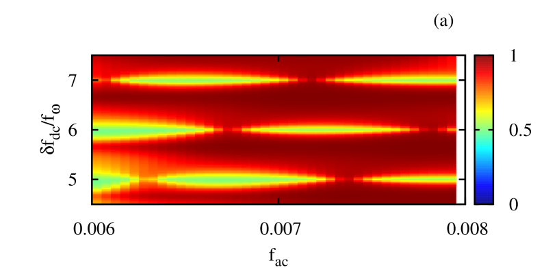
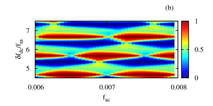
Figure 11: (Color online) An enlarged view of the same section of the first diamond shown in Fig.6 for the Ohmic bath. (a) For $\Omega_{p}=0.08$. (b) For $\Omega_{p}=0.02$

Regime (III): Sideband resonances. In this case, the two virtual crossings of $E_{1}$ with $E_{p0}$ are reached within the driving interval $\delta f_{dc}\pm f_{ac}$. This makes possible to access also the $E_{p1}$ level through Landau-Zener transitions at $\delta f=0$, which allows for new “sideband” resonances involving the $E_{p0}$ and $E_{p1}$ levels, in addition to the direct resonances at $E_{1}-E_{0}=n\omega_{0}$. When $E_{p1}-E_{0}=n\omega_{0}$, called a blue sideband resonance,milenas the qubit resonates between the $E_{0}$ and the $E_{p1}$ levels. However, the $E_{p1}$ virtual level is unstable and it decays to the $E_{1}$ level. In this way, the ac drive is continuously pumping population from the ground state to the excited state at $E_{1}$, leading to full inversion of the qubit population: ${\overline{P}}_{+}\sim 0$. When $E_{1}-E_{p0}=n\omega_{0}$, called a red sideband resonance,milenas the qubit resonates between the $E_{1}$ and the $E_{p0}$ levels. In this case, the $E_{p0}$ virtual level decays fast to the $E_{0}$ level, and thus the ac drive is continuously pumping population from the $E_{1}$ level to the ground state, leading to ${\overline{P}}_{+}\sim 1$. In Fig.11(b) we can see in detail the sideband resonance patterns that characterize this regime, with alternating $P_{+}\sim 0$ and $P_{+}\sim 1$. This type of resonances have been analyzed in Ref.milenas, , within a perturbative approach for $\Omega_{p}<\omega_{0}$. In that case, only the regime (III) is realized. On the other hand, when $\Omega_{p}>\omega_{0}$ the three regimes described above are possible.

To observe the subdivision of the first diamond in the three regimes, the crossing of $E_{1}$ with $E_{p0}$ should occur before the avoided crossing of $E_{1}$ with $E_{2}$. This means that the condition $f_{p}<f_{01}$ is required, or $\Omega_{p}<4\pi I_{p}f_{01}$. For the typical flux qubit parameters considered in this work, this later condition corresponds to $\Omega_{p}\lesssim 0.15$. The SQUID detectors used in the measurements of Refs.berns1, ; oliver, ; valenzuela, have typically $\Omega_{p}\sim 10\rm{GHz}$, which is $\Omega_{p}\sim 0.2$ in our normalized units. Therefore in the case of these LZS interferometry experiments, the effects of the resonant mode at $\Omega_{p}$ are negligible, and everything is within the regime (I) of asymptotic asymmetric resonances. On the opposite side, the flux qubits studied in Ref.chiorescu2, have $\Omega_{p}\lesssim\Delta\lesssim\omega_{0}$, which situates them deeply in the case of the regime (III). In fact, the $n=1$ blue and red sideband resonances have been observed in Ref.chiorescu2, . However, in these devices the oscillator mode of the SQUID detector is strongly coupled to the qubit, while Eq. (9) is valid for weak coupling. A full analysis in this case has to consider a quantum oscillator with frequency $\Omega_{p}$ coupled to the qubit within the system hamiltonian, see Refs.chiorescu2, ; milenas, . In any case, our results show that it will be interesting to perform experiments on LZS interferometry using SQUID detectors with low $\Omega_{p}$ and weakly coupled to the qubit, to observe the three regimes shown in Figs.10 and 11.

IV Conclusions

To summarize, by performing a realistic modeling of the flux qubit we were able to analyze the time dependence of the LZS interference patterns (as a function of ac amplitude and dc detuning) taking into account decoherence and relaxation.

We found an important difference between the LZS patterns observed for the time scale of current experiments and those for the asymptotic long time limit: a symmetry change in their structure. This is a dynamic transition as a function of time from a LZS pattern with nearly symmetric multiphoton resonance lobes to antisymmetric multiphoton resonances. This transition is observable only when driving the system for very long times, after full relaxation with the bath degrees of freedom ($t\gg t_{r}$).

The large time scale separation, $t_{r}\gg t_{dec}$, present in the device of Ref.valenzuela, explains why in their case the asymptotic LZS pattern is beyond the experimental time window. It will be interesting if experiments could be carried out for longer driving times in this device. For example, measurements of curves of $P_{+}$ at growing time scales near a multiphoton resonance, could show the transition from symmetric to antisymmetric behavior.

Another interesting finding is the dependence of the LZS interference patterns on the frequency $\Omega_{p}$ of the SQUID detector. Different types of LZS interference patterns can arise, depending on the magnitude of $\Omega_{p}$. In particular, we showed that the resonant mode at $\Omega_{p}$ can impede the dynamic transition when $\Omega_{p}$ is of the order of the qubit gap, in the regime (II) discussed in Sec.IIID. In principle, the frequency $\Omega_{p}$ can be varied (in a small range) by varying the driving current of the SQUID detector chiorescu2 or with a variable shunt capacitor.

*

Appendix A Floquet-Markov formalism for the periodically driven flux qubit

A.1 Periodically driven isolated flux qubit

Since the FQ of Eq.(1) is driven with a magnetic flux $f(t)=f_{dc}+f_{ac}\sin(\omega_{0}t)$, the hamiltonian is time periodic ${\cal H}(t)={\cal H}(t+\tau)$, with $\tau=2\pi/\omega_{0}$. In this case, it is convenient to use the Floquet formalism, that allows to treat periodic forces of arbitrary strength and frequency. shirley ; grifoni-hanggi ; grifonih ; fds ; chu-floquet ; barnes2013 According to the Floquet theorem,shirley the solutions of the Schrödinger equation are of the form

$$|\Psi(t)\rangle=\sum_{\alpha}c_{\alpha}e^{-i\varepsilon_{\alpha}t/\hbar}|\alpha(t)\rangle,$$

where $c_{\alpha}$ are time independent coefficients and $\varepsilon_{\alpha}$ are the so-called quasienergies. The Floquet states $|\alpha(t)\rangle$ are time-periodic,

$$|\alpha(t)\rangle=|\alpha(t+\tau)\rangle$$

and satisfy the eigenvalue equation

$$\hat{H}_{F}(t)|\alpha(t)\rangle=\varepsilon_{\alpha}|\alpha(t)\rangle,$$

where $\hat{H}_{F}(t)={\cal H}(t)-i\hbar\partial/\partial t$ is defined as the Floquet hamiltonian. The time periodicity of ${\cal H}(t)$ and $|\alpha(t)\rangle$ makes convenient to use the Fourier representation,

$${\cal H}(t) = \sum_{k}{\cal H}_{k}e^{-ik\omega_{0}t}$$ (10)

$$|\alpha(t)\rangle = \sum_{k}|\alpha_{k}\rangle e^{-ik\omega_{0}t}$$ (11)

Therefore, we can rewrite the Floquet eigenvalue equation as:

$$\sum_{q}\left[{\cal H}_{k-q}-\hbar k\omega_{0}I\delta_{k,q}\right]|\alpha_{q}\rangle=\varepsilon_{\alpha}|\alpha_{k}\rangle$$ (12)

with $I$ the identity.

For the driven FQ, we write ${\cal H}(t)=\ {\cal H}_{0}+W(t)$ with ${\cal H}_{0}={\cal H}_{FQ}(f_{dc})$ the time independent part of the hamiltonian of Eq.(1), and

$$W(t) = \alpha E_{J}\sin[2\pi f_{ac}\sin{(\omega_{0}t)}]\sin(2\pi f_{dc}+2\varphi_{l})+$$

$$\!\!\!2\alpha E_{J}\sin^{2}[\pi f_{ac}\sin{(\omega_{0}t)}]\cos(2\pi f_{dc}+2\varphi_{l})\;.$$

In the energy eigenbasis of ${\cal H}_{0}$, given by ${\cal H}_{0}|n\rangle=E_{n}|n\rangle$, the Eq.(12) can be written as

$$\sum_{m,q}\left[(E_{n}-\hbar k\omega_{0})\delta_{kq}\delta_{nm}+W_{k-q}^{nm}\right]\langle m|\alpha_{q}\rangle=\varepsilon_{\alpha}\langle n|\alpha_{k}\rangle$$ (14)

with

$$W^{nm}_{k}=\frac{\omega_{0}}{2\pi}\int_{0}^{2\pi/\omega_{0}}\langle n\left|W(t)\right|m\rangle e^{ik\omega_{0}t}dt\;,$$ (15)

The static eigenvalues $E_{n}$ and eigenstates $|n\rangle$ are obtained by numerical diagonalization of ${\cal H}_{0}$, using $2\pi$-periodic boundary conditions on $\vec{\bf\varphi}=(\varphi_{1},\varphi_{2})$ and a discretization grid of $\Delta\varphi=2\pi/M$ (with $M=256$).foot1 Then, the $W^{nm}_{k}$ are evaluated from Eqs. (15) and (LABEL:vt1), where the matrix elements $\langle n|\sin{(2\pi f_{dc}+2\varphi_{l})}|m\rangle$ and $\langle n|\cos{(2\pi f_{dc}+2\varphi_{l})}|m\rangle$ have been calculated using the obtained eigenstates $|n\rangle$. In order to solve the Floquet eigenvalue problem numerically we have to truncate the Eq. (14) both in the Fourier indices $k,q$ and the in the number of energy levels of ${\cal H}_{0}$ considered.fds The truncated eigenproblem is of dimension $N_{d}=(2K+1)N_{l}$ where $K=max|q-k|$ is defined by the maximum value of the Fourier index and $N_{l}$ by the number of levels considered in the diagonalization of ${\cal H}_{0}$. The obtained Floquet states $\langle n|\alpha_{k}\rangle$ and quasienergies $\varepsilon_{\alpha}$ contain all the information to study the quantum dynamics of the system described above.

An alternative method, which is more efficient for large $N_{l}$, is to consider the time evolution operator $U(t_{2},t_{1})$, which in the Floquet representation can be expanded as

$$U(t_{2},t_{1})=\sum_{\alpha}e^{-i\epsilon_{\alpha}(t_{2}-t_{1})}|\alpha(t_{2})\rangle\langle\alpha(t_{1})|.$$

Since $|\alpha(t+\tau)\rangle=|\alpha(t)\rangle$, the Floquet state $|\alpha(t)\rangle$ is an eigenvector of $U(t+\tau,t)$ with eigenvalue $e^{-i\varepsilon_{\alpha}\tau}$. Therefore, it is possible to calculate the Floquet states and quasienergies from the diagonalization of $U(t+\tau,t)$. Numerically, one needs to compute the evolution operator $U(t,0)$ within a period, for $0\leq t\leq\tau$. Taking discretized time steps of length $\delta t=\tau/M_{\tau}$, we use the second-order Trotter-Suzuki approximation

$$U(t_{j+1},t_{j})\approx e^{-i{\cal H}_{0}\frac{\delta t}{2}}e^{-iW(t_{j}+\frac{\delta t}{2})\delta t}e^{-i{\cal H}_{0}\frac{\delta t}{2}}$$

for times $t_{j}=j\delta t$, and we compute the product $U(t_{n},0)=\Pi_{j=0}^{n-1}U(t_{j+1},t_{j})$ for $n\leq M_{\tau}$, starting with $U(0,0)=I$. The Floquet states are then obtained as eigenvectors of $U(\tau,0)\equiv U(t_{M_{\tau}},0)$. We diagonalize numerically the hermitian matrix $C=i(1+U)(1-U)^{-1}$, solving $C|\alpha(\tau)\rangle=c_{\alpha}|\alpha(\tau)\rangle$, where $c_{\alpha}={\rm cotan}(\varepsilon_{\alpha}\tau/2)$ and $|\alpha(0)\rangle=|\alpha(\tau)\rangle$, The Floquet states at any time are then calculated as $|\alpha(t_{n})\rangle=e^{i\varepsilon_{\alpha}t_{n}}U(t_{n},0)|\alpha(0)\rangle$, and their Fourier components $|\alpha_{k}\rangle$ can be obtained using a fast Fourier transform routine. We find that for $N_{l}\geq 4$ this numerical procedure is more efficient than the direct diagonalization of Eq.(14).

Experimentally, the probability of having a state of positive or negative persistent current in the flux qubit is measured.chiorescu ; oliver ; valenzuela The probability of a positive current measurement (“right” side of the double-well potential) can be calculated, for $\delta f\ll 1$, integrating the probability $|\Psi(\varphi_{l},\varphi_{t})|^{2}$ within the subspace with $\pi>\varphi_{l}>0$:fds

$$P_{+}(t)=\int_{0}^{\pi}d\varphi_{l}\int_{-\pi}^{\pi}d\varphi_{t}\;|\Psi(\vec{\varphi})|^{2},$$

where $\vec{\varphi}=(\varphi_{l},\varphi_{t})$ and $\Psi(\vec{\varphi})=\langle\vec{\varphi}|\Psi\rangle$. For later generalizations, it is better to define the projector corresponding to a positive current measurement:

$$\hat{\Pi}_{+}=\int_{\pi>\varphi_{l}>0}d\vec{\varphi}\;|\vec{\varphi}\rangle\langle\vec{\varphi}|,$$

in terms of this operator, we have $P_{+}(t)=\langle\Psi(t)|\hat{\Pi}_{+}|\Psi(t)\rangle\equiv\langle\hat{\Pi}_{+}\rangle$. For an initial condition $|\Psi_{0}\rangle$ at $t_{0}$, we can express $P_{+}(t)$ in the Floquet basis as

$$P_{+}(t)=\sum_{\alpha,\beta}e^{-i(\varepsilon_{\alpha}-\varepsilon_{\beta})(t-t_{0})}\langle\alpha(t_{0})|\Psi_{0}\rangle\langle\Psi_{0}|\beta(t_{0})\rangle\pi_{\beta\alpha}(t)$$

with $\pi_{\beta\alpha}(t)=\langle\beta(t)|\hat{\Pi}_{+}|\alpha(t)\rangle$. In experiments the initial time, or equivalently the initial phase of the driving field seen by the system in repeated realizations of the measurement, is not well defined. Then, the quantities of interest are the probabilities averaged over initial times, $t_{0}$.shirley ; fds ; chu-floquet Using the properties of the Floquet functions, the average over the initial phase time $t_{0}$ gives

$$\overline{e^{i(\varepsilon_{\alpha}-\varepsilon_{\beta})t_{0}}|\beta(t_{0})\rangle\langle\alpha(t_{0})|}\rightarrow\delta_{\alpha\beta}\sum_{k}|\alpha_{k}\rangle\langle\alpha_{k}|,$$

and we obtain,

$$P_{+}(t)=\sum_{\alpha}{\pi_{\alpha\alpha}(t)\left[\sum_{k}|\langle\alpha_{k}|\Psi_{0}\rangle|^{2}\right]}$$

It is worth noticing that averaging over the initial phase time of the driving field is equivalent to defining a density matrix $\rho(t)=\overline{|\Psi(t)\rangle\langle\Psi(t)|}$ which, due to the average over $t_{0}$, is diagonal in the Floquet basis, $\rho_{\alpha\beta}=\langle\alpha(t)|\rho(t)|\beta(t)\rangle=\delta_{\alpha\beta}\sum_{k}|\langle\alpha_{k}|\Psi_{0}\rangle|^{2}$.

Finally, we average within a period over the observation time $t$, to obtain a time independent “stationary” probability $\overline{P}_{+}\equiv\overline{P_{+}(t)}$. After defining the time-averaged projector in the Floquet basis as

$$\overline{\pi}_{\alpha\beta}=\overline{\langle\alpha(t)|\hat{\Pi}_{+}|\beta(t)\rangle}=\sum_{k}\langle\alpha_{k}|\hat{\Pi}_{+}|\beta_{k}\rangle$$

we obtain the simple result

$$\overline{P}_{+}=\sum_{\alpha}\overline{\pi}_{\alpha\alpha}\rho_{\alpha\alpha}$$

with $\rho_{\alpha\alpha}=\sum_{k}|\langle\alpha_{k}|\Psi_{0}\rangle|^{2}$. Numerically, after diagonalization of ${\cal H}_{0}$ we compute the matrix elements of the projector $\pi_{nm}=\langle n|\hat{\Pi}_{+}|m\rangle=\int_{\pi>\varphi_{l}>0}\Phi_{n}^{*}(\vec{\varphi})\Phi_{m}(\vec{\varphi})d\vec{\varphi}$, with $\Phi_{n}(\vec{\varphi})=\langle\vec{\varphi}|n\rangle$.fds Then, for each $\omega_{0}$ and $f_{ac}$ the Floquet states and quasienergies are obtained, and the coefficients $\overline{\pi}_{\alpha\beta}=\sum_{k,n,m}\pi_{n,m}\alpha_{k,n}^{*}\beta_{k,m}$ are evaluated (with $\alpha_{k,n}=\langle n|\alpha_{k}\rangle$).

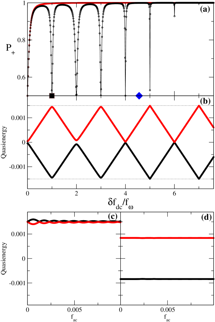
Figure 12: (Color online) (a) Probability $\overline{P}_{+}$ of a state with positive loop current as a function of $\delta f_{dc}$ for the undriven qubit (red squares) and for the driven qubit (black circles) with $f_{ac}=0.0001$ and $\hbar\omega_{0}/E_{J}=0.0003$. The flux detuning $\delta f_{dc}$ is normalized by $f_{\omega}=\omega_{0}/4\pi I_{p}$, such that the $n$-photon resonances are at $\delta f=nf_{\omega}$. (b) Floquet quasienergies (in units of $E_{J}$) as a function of $\delta f_{dc}$ for the same case as in (a). (c) Floquet quasienergies (in units of $E_{J}$) as a function of $f_{ac}$ for the $n=1$ resonant state at $f_{dc}=0.50033$ [corresponding to black square in panel (a)]. (d) Floquet quasienergies (in units of $E_{J}$) as a function of $f_{ac}$ for an out of resonance state at $f_{dc}=0.50151$ [corresponding to blue diamond in panel (a)]. Device parameters of the flux qubit are $\alpha=0.8$ and $\eta=0.25$.

As an example, we calculate ${P}_{+}$ for the driven FQ in the two-level regime, as described by the hamiltonian ${\cal H}_{FQ}\approx{\cal H}_{TLS}$ of Eq.(3). At zero temperature and in the absence of driving ($f_{ac}=0$) the isolated FQ is in the ground state. In this case, the probability $P_{+}$ is simply the projection of the ground state on the subspace of positive persistent current, and we have $P_{+}=\langle 0|\hat{\Pi}_{+}|0\rangle=\pi_{00}$. For $\delta f_{dc}=f_{dc}-1/2>0$ we have $P_{+}\approx 1$ except near $\delta f_{dc}=0$ where $P_{+}=1/2$, as can be seen in Fig.12(a). (While for $\delta f_{dc}<0$, we have $P_{+}\approx 0$, since the ground state has the loop current in the opposite direction in this case). In the presence of an ac drive, $\delta f(t)=\delta f_{dc}+f_{ac}\cos(\omega_{0}t)$, we calculate the time averaged ${\overline{P}}_{+}$, following the procedure discussed above. The time averaged ${\overline{P}}_{+}$ vs. $f_{dc}$ shows dips corresponding to $n-$photon resonances. as shown in Fig.12(a). These $n$-resonances are at $\epsilon_{0}\approx n\omega_{0}$, which is equivalent to $\delta f_{dc}=nf_{\omega}$, after defining $f_{\omega}=\omega_{0}/4\pi I_{p}$. the $n$-resonances are at $\delta f_{dc}=nf_{\omega}$. In the Floquet picture, these resonances correspond to avoided crossings of the Floquet quasienergiesgrifoni-hanggi ; grifonih as a function of $\delta f_{dc}$ as we illustrate in Fig.12(b). When increasing $f_{ac}$, we see that for a $n$-resonance the quasienergies have a small gap, $|\varepsilon_{\alpha}-\varepsilon_{\beta}|\ll\omega_{0}$ (with the difference $\varepsilon_{\alpha}-\varepsilon_{\beta}$ defined modulo $\omega_{0}$). On the other hand, for a value of $\delta f_{dc}$ away of a resonance the quasienergies maintain a finite gap (compared to $\omega_{0}$) as a function of $f_{ac}$, see Fig.12(c) and (d).

A.2 Floquet-Markov approach for open system

Experimentally, the system is affected by the electromagnetic environment that introduces decoherence and relaxation processes. A standard theoretical model to study enviromental effects is to couple the system bilinearly to a bath of non-interacting harmonic oscillators with masses $m_{\nu}$, frequencies $\omega_{\nu}$, momenta $p_{\nu}$, and coordinates $x_{\nu}$, with the coupling strength $\gamma_{\nu}$.grifoni-hanggi The total Hamiltonian of system and bath is then given by

$${\cal H}={\cal H}_{S}(t)+{\cal H}_{SB}+{\cal H}_{B}$$

where ${\cal H}_{S}(t)$ is the time-periodic Hamiltonian of the system, $H_{B}$ is the Hamiltonian that describes a bath of harmonic oscillators and $H_{SB}$ its system-bath coupling Hamiltonian term,

$${\cal H_{B}}=\sum_{\nu=1}^{\infty}\left[\frac{p_{\nu}^{2}}{2m_{\nu}}+\frac{m_{\nu}\omega_{\nu}^{2}x_{\nu}^{2}}{2}\right]$$ (16)

$${\cal H_{SB}}=\hat{A}\sum_{\nu=1}^{\infty}\gamma_{\nu}x_{\nu}$$ (17)

with $\hat{A}$ the operator of the system that couples to the bath. The bath degrees of freedom are characterized by the spectral density

$$J(\omega)=\pi\sum_{\nu=1}^{\infty}\frac{\gamma_{\nu}^{2}}{2m_{\nu}\omega_{\nu}}\delta(\omega-\omega_{\nu}).$$

It is further assumed that at time $t=0$ the bath is in thermal equilibrium and uncorrelated to the system. Then, the full density matrix $\sigma(t)$ has at initial time the form $\sigma(0)=\rho(0)\exp(-\beta H_{B})/tr_{B}\exp(-\beta H_{B})$, where $\rho(t)={\rm Tr}_{B}(\sigma)$ is the density matrix of the system and $T=1/(k_{B}\beta)$ is the bath temperature. After expanding the density matrix of the system in the time-periodic Floquet states

$$\rho_{\alpha\beta}(t)=\langle\alpha(t)|\rho(t)|\beta(t)\rangle\;,$$ (18)

the Born (weak coupling) and Markov (fast relaxation) approximations for the time evolution of $\rho_{\alpha\beta}(t)$ are performed. In this way, the Floquet-Markov master equation is obtainedgrifoni-hanggi ; grifonih ; hanggi ; breuer ; ketzmerich ; fazio1 ; solinas2

$$\frac{d\rho_{\alpha\beta}(t)}{dt}=-\frac{i}{\hbar}(\varepsilon_{\alpha}-\varepsilon_{\beta})\rho_{\alpha\beta}(t)+\sum_{\alpha^{\prime}\beta^{\prime}}{\cal L}_{\alpha\beta\alpha^{\prime}\beta^{\prime}}(t)\rho_{\alpha^{\prime}\beta^{\prime}}(t)$$ (19)

The first term in Eq.(19) represents the nondissipative dynamics and the influence of the bath is described by the time-dependent rate coefficients

$${\cal L}_{\alpha\beta\alpha^{\prime}\beta^{\prime}}(t)=\sum_{q}{\cal L}^{q}_{\alpha\beta\alpha^{\prime}\beta^{\prime}}e^{-iq\omega_{0}t}$$ (20)

with

$${\cal L}^{q}_{\alpha\beta\alpha^{\prime}\beta^{\prime}}=\sum_{k}\left(g_{\alpha\alpha^{\prime}}^{k}+g_{\beta\beta^{\prime}}^{-k-q}\right)A_{\alpha\alpha^{\prime}}^{k}A_{\beta^{\prime}\beta}^{k+q}-$$

$$\delta_{\beta\beta^{\prime}}\sum_{\eta}g_{\eta\alpha^{\prime}}^{k}A_{\alpha\eta}^{k+q}A_{\eta\alpha^{\prime}}^{k}-$$

$$\delta_{\alpha\alpha^{\prime}}\sum_{\eta}g_{\eta\beta^{\prime}}^{-k}A_{\eta\beta}^{k+q}A_{\beta^{\prime}\eta}^{k}$$ (21)

The nature of the bath is encoded in the coefficients

$$g_{\alpha\beta}^{q}=J(\varepsilon_{\alpha\beta}^{q}/{\hbar})n_{\rm th}(\varepsilon_{\alpha\beta}^{q})$$

with $\varepsilon_{\alpha\beta}^{q}=\varepsilon_{\alpha}-\varepsilon_{\beta}+q\hbar\omega_{0}$ and $n_{\rm th}(x)=1/(\exp{(x/k_{B}T)}-1)$, and defining $J(-x)=-J(x)$ for $x<0$. The system-bath interaction is encoded in the transition matrix elements $A_{\alpha\beta}^{k}$ in the Floquet basis

$$A_{\alpha\beta}^{q}=\sum_{k}\langle\alpha_{k}|\hat{A}|\beta_{k+q}\rangle$$

In the case of the driven FQ, the system hamiltonian is ${\cal H}_{S}={\cal H}_{FQ}(t)$ and the bath degrees of freedom couple with the system variable $\varphi_{l}$ since the dominating source of decoherence is flux noise (see Ref.caspar, ). Thus, after taking $\hat{A}=\varphi_{l}$ and in terms of the eigenbasis of $H_{0}$, we have to compute

$$A_{\alpha\beta}^{q}=\sum_{nm}\sum_{k}\alpha_{k,n}^{*}\beta_{k+q,m}\langle n|\varphi_{l}|m\rangle.$$ (22)

Considering that the time scale $t_{r}$ for full relaxation satisfies $t_{r}\gg\tau$, the transition rates ${\cal L}_{\alpha\beta\alpha^{\prime}\beta^{\prime}}(t)$ can be approximated by their average over one period $\tau$, hanggi ${\cal L}_{\alpha\beta\alpha^{\prime}\beta^{\prime}}(t)\approx{\cal L}^{q=0}_{\alpha\beta\alpha^{\prime}\beta^{\prime}}={\it L}_{\alpha\beta\alpha^{\prime}\beta^{\prime}}$, obtaining

$${\it L}_{\alpha\beta\alpha^{\prime}\beta^{\prime}} = R_{\alpha\beta\alpha^{\prime}\beta^{\prime}}+R_{\beta\alpha\beta^{\prime}\alpha^{\prime}}^{*}$$

$$-\sum_{\eta}\left(\delta_{\beta\beta^{\prime}}R_{\eta\eta\alpha^{\prime}\alpha}+\delta_{\alpha\alpha^{\prime}}R_{\eta\eta\beta^{\prime}\beta}^{*}\right).$$

The rates

$$R_{\alpha\beta\alpha^{\prime}\beta^{\prime}}=\sum_{q}g_{\alpha\alpha^{\prime}}^{q}A_{\alpha\alpha^{\prime}}^{q}A_{\beta^{\prime}\beta}^{-q}$$ (24)

can be interpreted as sums of $q$-photon exchange terms.

This formalism has been extensively employed to study relaxation and decoherence for time dependent periodic evolutions in double-well potentials and in two level systems.grifoni-hanggi ; grifonih ; hanggi ; breuer ; ketzmerich Here we use it to model the ac driven FQ, considering the full multilevel Hamiltonian of Eq. (1).fds2

The probability of a positive current measurement is calculated as $P_{+}(t)=\langle\hat{\Pi}_{+}\rangle={\rm Tr}(\hat{\Pi}_{+}\rho(t))$, with $\hat{\Pi}_{+}$ the projector defined in the previous section. With $\rho(t)$ calculated in the Floquet basis is

$$P_{+}(t)=\sum_{\alpha,\beta}\pi_{\beta\alpha}(t)\rho_{\alpha\beta}(t)$$ (25)

To calculate the time dependence of $\rho_{\alpha\beta}(t)$ it is convenient to work in the superoperator formalism of the so-called Liouville space.blum ; pollard We write,

$$\frac{d\rho_{\alpha\beta}(t)}{dt}=\sum_{\alpha^{\prime}\beta^{\prime}}\Lambda_{\alpha\beta\alpha^{\prime}\beta^{\prime}}\;\rho_{\alpha^{\prime}\beta^{\prime}}$$

with $\Lambda_{\alpha\beta\alpha^{\prime}\beta^{\prime}}=-\frac{i}{\hbar}(\varepsilon_{\alpha}-\varepsilon_{\beta})\delta_{\alpha\alpha^{\prime}}\delta_{\beta\beta^{\prime}}+L_{\alpha\beta\alpha^{\prime}\beta^{\prime}}$. Then we change notation rewriting the $N_{l}\times N_{l}$ matrix $\rho$ as an $N_{l}^{2}\times 1$ vector represented as the ket $|\rho\rangle\rangle$, and the $N_{l}^{2}\times N_{l}^{2}$ “supermatrix” $\Lambda_{\alpha\beta\alpha^{\prime}\beta^{\prime}}$ as the operator $\hat{\Lambda}$ acting on this linear space, where the inner product is defined as $\langle\langle\sigma|\rho\rangle\rangle={\rm Tr}(\sigma^{\dagger}\rho)$. In particular, for the identity matrix $I$ we have $\langle\langle I|\rho\rangle\rangle=\langle\langle\rho|I\rangle\rangle={\rm Tr}(\rho)=1$, the later equality corresponding to the normalization of $\rho$, which is a conserved quantity. On the other hand, the norm of the vector $|\rho\rangle\rangle$ is $|||\rho\rangle\rangle||=\sqrt{{\rm Tr}(\rho^{2})}\leq 1$. In this notation, we can rewrite the Floquet-Markov equation as

$$\frac{d|\rho\rangle\rangle}{dt}=\hat{\Lambda}|\rho\rangle\rangle$$ (26)

The superoperator $\hat{\Lambda}$ is non-hermitian and has left and right eigenvectors with complex eigenvalues $\lambda_{\mu}$,

$$\hat{\Lambda}|r_{\mu}\rangle\rangle = \lambda_{\mu}|r_{\mu}\rangle\rangle$$ (27)

$$\langle\langle l_{\mu}|\hat{\Lambda} = \langle\langle l_{\mu}|\lambda_{\mu}$$ (28)

which are mutually orthogonal, $\langle\langle l_{\mu}|r_{\nu}\rangle\rangle=\delta_{\mu\nu}$. In general, the number of independent eigenvectors of $\hat{\Lambda}$ can be less than the dimensionality of $\hat{\Lambda}$. A formal solution of Eq.(26) for $|\rho(t)\rangle\rangle$ can be obtained using a similarity transformation to the Jordan normal form of $\hat{\Lambda}$.lendi ; baumgartner ; albert In the cases considered in this work we found numerically that it was always possible to diagonalize $\hat{\Lambda}$, in which case the solution of Eq.(26) can be expressed as

$$|\rho(t)\rangle\rangle = \sum_{\mu}c_{\mu}e^{\lambda_{\mu}t}|r_{\mu}\rangle\rangle$$ (29)

$$c_{\mu} = \langle\langle l_{\mu}|\rho(0)\rangle\rangle$$ (30)

from where we can calculate numerically $\rho_{\alpha\beta}(t)\equiv|\rho(t)\rangle\rangle_{\alpha\beta}$. The probability of a positive current measurement is then obtained combining Eq.(25) with Eq.(30).

The asymptotic state $|\rho(t\rightarrow\infty)\rangle\rangle\equiv|\rho^{\infty}\rangle\rangle$ satisfies,

$$\hat{\Lambda}|\rho^{\infty}\rangle\rangle=0$$

Therefore, the asymptotic state can be constructed from the right-eigenvectors $|r_{\mu}\rangle\rangle$ of $\hat{\Lambda}$ with eigenvalue $\lambda_{0}=0$ (i.e., the kernel of $\hat{\Lambda}$). If $\lambda_{0}$ is non-degenerate, then the asymptotic state is unique and independent of the initial condition $\rho(0)$. In the cases considered in this work we found, within the numerical accuracy, that the eigenvalue $\lambda_{0}=0$ was non-degenerate, and so the asymptotic state was given by the eigenvector $|r_{0}\rangle\rangle$, and then $\rho_{\alpha\beta}^{\infty}=|r_{0}\rangle\rangle_{\alpha\beta}$. The time independence of the asymptotic $\rho_{\alpha\beta}^{\infty}$, implies that quantities like $P_{+}$ in Eq(25), become time-periodic with period $\tau$ in the asymptotic state. Therefore, it is convenient to calculate the asymptotic $P_{+}(t)$ averaged over one period as

$$\overline{P_{+}}=\sum_{\alpha,\beta}\overline{\pi}_{\beta\alpha}|r_{0}\rangle\rangle_{\alpha\beta}$$ (31)

It is also clear from Eq.(30) that information about the relaxation and decoherence rates is contained in the non-zero eigenvalues $\lambda_{\mu}$ of $\hat{\Lambda}$.lendi ; baumgartner ; albert On one hand, the relaxation rates are given by the negative real eigenvalues of $\hat{\Lambda}$, where the long time relaxation rate $\Gamma_{r}=1/t_{r}$ is given by the minimum of $-Re(\lambda_{\mu})$ (excluding $\lambda_{0}=0$). On the other hand, the decoherence rates are given by the negative real parts of the complex conjugate pairs of eigenvalues of $\hat{\Lambda}$.

A.3 Decoherence in the Floquet basis

It is well known that the density matrix becomes diagonal in the energy basis for times larger than the relaxation time in undriven systems.blum In this case, the decay time of the offdiagonal $\rho_{nm}$ defines the decoherence time $\tau_{\phi}^{nm}$ between the eigenstates $E_{n}$ and $E_{m}$. For time scales $t\gg\tau_{\phi}^{nm}$, relaxation is described by the Pauli rate equation for the populations of the energy levels $P_{n}=\rho_{nn}$. In the case of a system with a time periodic drive, it is usually assumed that for large times the density matrix becomes approximately diagonal in the Floquet basis.grifoni-hanggi ; hanggi ; breuer ; ketzmerich ; fazio1 More precisely, this approximation can be justified when $\varepsilon_{\alpha}-\varepsilon_{\beta}\gg{\it L}_{\alpha^{\prime}\beta^{\prime}\alpha\beta}$, which is fulfilled for very weak coupling with the environment and away from resonances, see Ref.hanggi, ; fazio1, . From Fig.12(c) and (d) it is clear that this condition will be easily satisfied in the offresonant case considered here, where the Floquet gap $|\varepsilon_{\alpha}-\varepsilon_{\beta}|$ is large. On the other hand at an near a resonance where $|\varepsilon_{\alpha}-\varepsilon_{\beta}|\approx 0$ this condition can not be fulfilled, unless the system-bath coupling is extremely small.fazio1

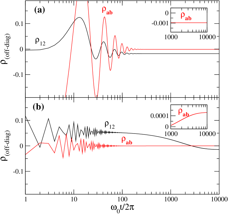
Figure 13: (Color online) Off-diagonal elements of the density matrix $\rho$ as a function of time. Black lines: off-diagonal matrix element $\rho_{12}$ in the basis of eigenstates of the undriven Hamiltonian. Red lines: off-diagonal element $\rho_{ab}$ in the Floquet basis. (a) For a resonant state at $f_{dc}=0.50099$ driven with $f_{ac}=0.0001$ and $\hbar\omega_{0}/E_{J}=0.0003$. (b) For an off-resonant state at $f_{dc}=0.50151$ driven with $f_{ac}=0.00245$ and $\hbar\omega_{0}/E_{J}=0.0003$. Insets in (a) and (b) show $\rho_{ab}$ at large times.

In Fig.13 we show the time evolution of matrix elements of $\rho$ calculated in the eigenbasis of $H_{0}$ and in the Floquet basis, both for an offresonant and for a resonant case. To clarify notation, for the $H_{0}$ eigenbasis we use latin indices $i,j$ with $i=1,2,3,\ldots$ ordered for increasing eigenenergy $E_{1}<E_{2}<E_{3}<\ldots$. For the Floquet basis we use greek indices $\alpha,\beta$ with $\alpha=a,b,c,\ldots$, and ordered such that $\alpha=a$ corresponds to the state that in the limit $f_{ac}\rightarrow 0$ maps to the ground state (with index $i=1$); $\alpha=b$ corresponds to the state that in the limit $f_{ac}\rightarrow 0$ maps to the first excited state (with index $i=2$), and so on.

The time dependence of the offdiagonal elements $\rho_{ij}$ in the the $H_{0}$ eigenbasis, are shown in Fig.13(a) and Fig.13(b) for the resonant and offresonant cases, respectively. (Here we consider the flux qubit in contact with an Ohmic bath with $J(\omega)=\gamma\omega$). We see that for long times $\rho_{ij}(t\rightarrow\infty)$ goes to a finite non-zero value that can not be neglected, showing explicitly that the driven system density matrix is not diagonal in the eigenenergy basis. Therefore approaches based on the use of the Pauli rate equation in the eigenenergy basis will not be correct for the analysis of the asymptotic long time behavior. In the case of the Floquet basis, we see in Fig.13(a) and (b) that the offdiagonal $\rho_{ab}$ after having oscillations at short time scales, decreases exponentially to very low values for long times. We find that $\rho_{ab}(t\rightarrow\infty)\approx 10^{-3}$ for the offresonant case (while diagonal elements $\rho_{\alpha\alpha}(t\rightarrow\infty)\sim 0.1-1$). This confirms that it is a good approximation to neglect the $\rho_{ab}$ at long times in this case. On the other hand, in the resonant case we find $\rho_{ab}^{\rm resonant}(t\rightarrow\infty)\approx 10^{-2}>\rho_{ab}^{\rm offresonant}(t\rightarrow\infty)$. Thus, in this case neglecting $\rho_{ab}$ is not a good approximation as in the offresonant case. The results reported in the main body of the paper correspond to the solution of the full Floquet-Markov equation, Eq. 26. However, we have verified that most of our results (including the dynamic transition discussed in Sec.III) are accurately reproduced by the approximation that assumes an asymptotic density matrix diagonal in the Floquet basis.

Assuming that the density matrix becomes diagonal in the Floquet basis, one can separate the dynamics of the diagonal and the off-diagonal density matrix. The off-diagonal part is dominated by the dependence

$$\frac{d\rho_{\alpha\beta}}{dt}\approx\left[-\frac{i}{\hbar}(\varepsilon_{\alpha}-\varepsilon_{\beta})+L_{\alpha\beta\alpha\beta}\right]\,\rho_{\alpha\beta}\;\;\;\;\alpha\not=\beta$$

In this approximation, the decoherence rate between the $|\alpha\rangle$ and the $|\beta\rangle$ Floquet state, is given by $\Gamma_{\alpha\beta}=-L_{\alpha\beta\alpha\beta}$. The dynamics for the diagonal part of the density matrix gives a rate equation for the population of the Floquet states $P_{\alpha}=\rho_{\alpha\alpha}$:

$$\frac{dP_{\alpha}}{dt} = \sum_{\beta}L_{\alpha\alpha\beta\beta}P_{\beta}$$ (32)

$$= 2\sum_{\beta}R_{\alpha\alpha\beta\beta}P_{\beta}-R_{\beta\beta\alpha\alpha}P_{\alpha}$$

where $R_{\alpha\alpha\beta\beta}=\sum_{n}g_{\alpha\beta}^{n}|A_{\alpha\beta}^{n}|^{2}$, after Eq. (24). It is simple to solve the above rate equation when we restrict to two levels. With two Floquet states $|a\rangle,|b\rangle$, the asymptotic populations are $P_{a}^{\infty}=R_{aabb}/(R_{aabb}+R_{bbaa})$, $P_{b}^{\infty}=1-P_{a}^{\infty}$; and the relaxation rate is $\Gamma_{r}=2(R_{aabb}+R_{bbaa})$. Using Eq.(24), we can decompose the relaxation rate as a sum of terms that describe virtual n-photon transitions:grifonih

$$\Gamma_{r}=\Gamma^{(0)}+\sum_{n\not=0}\Gamma^{(n)}\;,$$ (33)

with

$$\Gamma^{(n)}=2(g_{ab}^{n}|A_{ab}^{n}|^{2}+g_{ba}^{n}|A_{ba}^{n}|^{2}).$$ (34)

References

- (1) S.N. Shevchenko, S. Ashhab and Franco Nori, Phys. Rep. 492, 1 (2010).
- (2) S. Yoakum, L. Sirko, and P. M. Koch, Phys. Rev. Lett. 69, 1919 (1992).
- (3) W. D. Oliver, Y. Yu, J. C. Lee, K. K. Berggren, L. S. Levitov, and T. P. Orlando, Science 310, 1653 (2005);
- (4) D. M. Berns, W. D. Oliver, S. O. Valenzuela, A. V. Shytov, K. K. Berggren, L. S. Levitov, and T. P. Orlando, Phys. Rev. Lett. 97, 150502 (2006).
- (5) M. S. Rudner, A. V. Shytov, L. S. Levitov, D. M. Berns, W. D. Oliver, S. O. Valenzuela, and T. P. Orlando Phys. Rev. Lett. 101, 190502 (2008).
- (6) D. M. Berns, M. S. Rudner, S. O. Valenzuela, K. K. Berggren, W. D. Oliver, L. S. Levitov, and T. P. Orlando, Nature 455, 51 (2008); W D. Oliver and S. O. Valenzuela, Quantum Inf. Process 8, 261 (2009).
- (7) A. Izmalkov, S. H. W. van der Ploeg, S. N. Shevchenko, M. Grajcar, E. Il’ichev, U. Hb̈ner, A. N. Omelyanchouk, and H.-G. Meyer1, Phys. Rev. Lett. 101, 017003 (2008).
- (8) M. Sillanpaa, T. Lehtinen, A. Paila, Y. Makhlin, and P. Hakonen, Phys. Rev. Lett. 96, 187002 (2006).
- (9) C. M. Wilson, T. Duty, F. Persson, M. Sandberg, G. Johansson, and P. Delsing, Phys. Rev. Lett. 98, 257003 (2007).
- (10) C. M. Wilson, G. Johansson, T. Duty, F. Persson, M. Sandberg, and P. Delsing Phys. Rev. B 8̱1, 024520 (2010).
- (11) G. Z. Sun et al, Appl. Phys. Lett. 94, 102502 (2009).
- (12) Guozhu Sun, Xueda Wen, Bo Mao, Yang Yu, Jian Chen, Weiwei Xu, Lin Kang, Peiheng Wu, and Siyuan Han, Phys. Rev. B 83, 180507(R) (2011).
- (13) Yiwen Wang, Shanhua Cong, Xueda Wen, Cheng Pan, Guozhu Sun, Jian Chen, Lin Kang, Weiwei Xu, Yang Yu, and Peiheng Wu Phys. Rev. B 81, 144505 (2010).
- (14) S. E. de Graaf, J. Leppäkangas, A. Adamyan, A. V. Danilov, T. Lindström, M. Fogelström, T. Bauch, G. Johansson, and S. E. Kubatkin Phys. Rev. Lett. 111, 137002 (2013).
- (15) S. N. Shevchenko, A. N. Omelyanchouk, and E. Il’ichev Low Temp. Phys. 38 283 (2012)
- (16) M. Mark, T. Kraemer, P. Waldburger, J. Herbig, C. Chin, H.-C. Nägerl, and R. Grimm, Phys. Rev. Lett. 99, 113201 (2007).
- (17) J. R. Petta, H. Lu, and A. C. Gossard, Science 327, 669 (2010).
- (18) J. Stehlik, Y. Dovzhenko, J. R. Petta, J. R. Johansson, F. Nori, H. Lu, and A. C. Gossard Phys. Rev. B 86, 121303(R) (2012).
- (19) Gang Cao, Hai-Ou Li, Tao Tu, Li Wang, Cheng Zhou, Ming Xiao, Guang-Can Guo, Hong-Wen Jiang, and Guo-Ping Guo Nat Comms 4 1401 (2013).
- (20) E. Dupont-Ferrier, B. Roche, B. Voisin, X. Jehl, R. Wacquez, M. Vinet, M. Sanquer, and S. De Franceschi Phys. Rev. Lett. 110, 136802 (2013).
- (21) Runan Shang, Hai-Ou Li, Gang Cao, Ming Xiao, Tao Tu, Hongwen Jiang, Guang-Can Guo, and Guo-Ping Guo Appl. Phys. Lett. 103 162109 (2013).
- (22) P. Nalbach, J. Knörzer, and S. Ludwig Phys. Rev. B 87, 165425 (2013)
- (23) F. Forster, G. Petersen, S. Manus, P. Hänggi, D. Schuh, W. Wegscheider, S. Kohler, and S. Ludwig Phys. Rev. Lett. 112, 116803 (2014)
- (24) J.I. Colless, X.G. Croot, T.M. Stace, A.C. Doherty, S.D. Barrett, H. Lu, A.C. Gossard, and D.J. Reilly Nat Comms 5 (2014).
- (25) G. Granger, G. C. Aers, S. A. Studenikin, A. Kam, P. Zawadzki, Z. R. Wasilewski, and A. S. Sachrajda Phys. Rev. B 91, 115309 (2015).
- (26) Pu Huang, Jingwei Zhou, Fang Fang, Xi Kong, Xiangkun Xu, Chenyong Ju, and Jiangfeng Du, Phys. Rev. X 1, 011003 (2011).
- (27) J. Zhou, P. Huang, Q. Zhang, Z. Wang, T. Tan, X. Xu, F. Shi, X. Rong, S. Ashhab, and J. Du, Phys. Rev. Lett.112, 010503 (2014).
- (28) M. D. LaHaye, J. Suh, P. M. Echternach, K. C. Schwab, and M. L. Roukes, Nature (London) 459, 960 (2009).
- (29) Sebastian Kling, Tobias Salger, Christopher Grossert, and Martin Weitz, Phys. Rev. Lett. 105, 215301 (2010)
- (30) J. Bylander, M. Rudner, A. Shytov, S. Valenzuela, D. Berns, K. Berggren, L. Levitov, and W. Oliver, Phys. Rev. B 80, 220506 (2009).
- (31) Simon Gustavsson, Jonas Bylander,and William D. Oliver, Phys. Rev. Lett. 110, 016603 (2013).
- (32) A. M. Satanin, M. V. Denisenko, A. I. Gelman, and Franco Nori Phys. Rev. B 90 104516 (2014).
- (33) Ralf Blattmann, Peter Hanggi, and Sigmund Kohler, Phys. Rev. A 91, 042109 (2015).
- (34) Shuang Xu, Yang Yu, Guozhu Sun, Phys. Rev. B 82, 144526 (2010).
- (35) M. P. Silveri, K. S. Kumar, J. Tuorila, J. Li, A. Vepsalainen, E. V. Thuneberg, and G. S. Paraoanu, New J. Phys. 17, 043058 (2015).
- (36) A. M. Satanin, M. V. Denisenko, Sahel Ashhab, and Franco Nori Phys. Rev. B 85, 184524 (2012).
- (37) Georg Heinrich, J. G. E. Harris, and Florian Marquardt Phys. Rev. A 81, 011801(R)(2010); Huaizhi Wu, Georg Heinrich and Florian Marquardt, New Journal of Physics 15, 123022 (2013).
- (38) S. Gasparinetti, P. Solinas, and J. P. Pekola Phys. Rev. Lett. 107, 207002 (2011), Xinsheng Tan, Dan-Wei Zhang, Zhentao Zhang, Yang Yu, Siyuan Han, and Shi-Liang Zhu Phys. Rev. Lett. 112, 027001 (2014), Junhua Zhang, Jingning Zhang, Xiang Zhang, and Kihwan Kim, Phys. Rev. A 89, 013608 (2014).
- (39) X. Wen and Y. Yu, Phys. Rev. B. 79, 094529 (2009).
- (40) F. Grossmann, T. Dittrich, P. Jung, and P. H¨anggi, Phys. Rev. Lett. 67, 516 (1991); F. Grossmann and P. Hänggi, Europhys. Lett. 18, 571 (1992).
- (41) Y. Kayanuma, Phys. Rev. A 50, 843 (1994).
- (42) J. H. Shirley, Phys. Rev. 138, B979 (1965).
- (43) S. Ashhab, J.R. Johansson, A.M. Zagoskin, and Franco Nori, Phys. Rev. A 75, 063414 (2007).
- (44) M. Grifoni and P. Hänggi, Phys. Rep. 304, 229 (1998).
- (45) L. Hartmann et al, Phys. Rev. E 61, R4687 (2000).
- (46) Yu. Dakhnovskii and R.D. Coalson, J. Chem. Phys. 103, 2908 (1995); I.A. Goychuk, E.G. Petrov, and V. May, Chem. Phys. Lett. 253, 428 (1996).
- (47) M. C. Goorden and F. K. Wilhelm, Phys. Rev. B 68, 012508 (2003).
- (48) J. Hausinger and M. Grifoni, Phys. Rev. A 81, 022117 (2010).
- (49) T.M. Stace, A. C. Doherty, and S. D. Barrett, Phys. Rev. Lett. 95, 106801 (2005).
- (50) A. Ferrón, D. Domínguez and M. J. Sánchez, Phys. Rev. Lett. 109, 237005 (2012).
- (51) Y. Makhlin, G. Schön, and A. Shnirman, Rev. Mod. Phys. 73, 357 (2001). ; G. Wendin and V. Shumeiko, Low Temp. Phys. 33, 724 (2007).
- (52) J. Q. You and F. Nori, Nature 474, 589 (2011).
- (53) J. E. Mooij, T.P.Orlando, L.S. Levitov, L. Tian, C.H. van der Wal and S. Lloyd, Science 285, 1036 (1999); T.P.Orlando, J.E. Mooij, L. Tian, C.H. van der Wal, L.S. Levitov, S. Lloyd, J.J. Mazo, Phys. Rev. B 60, 15398 (1999).
- (54) I. Chiorescu, Y. Nakamura, C. J. P. M. Harmans, and J. E. Mooij, Science 299, 1869 (2003).
- (55) I. Chiorescu et al., Nature (London) 431, 159 (2004); J. Johansson et al, Phys. Rev. Lett. 96, 127006 (2006)
- (56) We diagonalized the Hamiltonian using the representation in terms of and periodic boundary conditions in the wave function . The discretization grid is , with , and the lowest eigenvalues and eigenvectors are obtained with a Lanczos algorithm, employing the ARPACK library.
- (57) For low energies, the potential is approximately separable in the longitudinal [] and transverse [] directions near the two minima. Therefore, at low energies the first eigenstates can be assigned longitudinal and transverse quantum numbers. The black curves in Fig.1 correspond to eigenstates with the lowest transverse mode, i.e. wave functions symmetric in . The blue curves in Fig.1 correspond to eigenstates with higher transverse modes, not necessarily symmetric in . The driving in is along the longitudinal direction and therefore conserves the parity of the transverse modes. The avoided crossings indicated as in Fig.1 have a negligibly small gap .
- (58) A. Ferrón and D. Dominguez, Phys. Rev. B 81, 104505 (2010).
- (59) A. Ferrón, D. Domínguez and M. J. Sánchez, Phys. Rev. B. 82,134522 (2010).
- (60) L. Du, M. Wang, Y. Yu., Phys. Rev. B 82, 045128 (2010).
- (61) L. Du, Y. Yu., Phys. Rev. B 82, 144524 (2010)
- (62) C. H. van der Wal, F. K. Wilheim, C. J. P. M. Harmans, and J. E. Mooij. Eur. Phys. J. B 31, 111 (2003).
- (63) M. C. Goorden, M. Thorwart and M. Grifoni, Phys. Rev. Lett. 93, 267005 (2004); Eur. Phys. J. B 45, 405 (2005).
- (64) A. Garg, J. N. Onuchic, and V. Ambegaokar, J. Chem. Phys. 83, 4491 (1985).
- (65) Sang-Kil Son, Siyuan Han and Shih-I Chu, Phys. Rev. A 79, 032301 (2009); S. I. Chu and D. A. Telnov, Phys. Rep. 390, 1 (2004); D. A Telnov and S. I. Chu, Phys. Rev. A, 71, 013408 (2005).
- (66) Sriram Ganeshan, Edwin Barnes, and S. Das Sarma Phys. Rev. Lett. 111 130405 (2013).
- (67) S. Kohler, T. Dittrich and P. Hänggi, Phys. Rev. E. 55, 300 (1997). S. Kohler, R. Utermann, P. Hänggi, and T. Dittrich, Phys. Rev. E. 58, 7219 (1998).
- (68) H.-P. Breuer, W. Huber and F. Petruccione, Phys. Rev. E 61, 4883 (2000).
- (69) D. W. Hone, R. Ketzmerick and W. Kohn, Phys. Rev. E 79, 051129 (2009).
- (70) S. Gasparinetti, P. Solinas, S. Pugnetti, R. Fazio, and J. Pekola Phys. Rev. Lett. 110 150403 (2013).
- (71) Vera Gramich, Simone Gasparinetti, Paolo Solinas, and Joachim Ankerhold Phys. Rev. Lett. 113, 027001 (2014).
- (72) K. Blum, Density matrix theory and applications, Springer; 3rd edition ( 2012).
- (73) W. Thomas Pollard and Richard A. Friesner, J. Chem. Phys. 100, 5054 (1994); W. Thomas Pollard, Anthony K. Felts, and Richard A. Friesner,Advances in Chemical Physics, Volume XCIII, Edited by I. Prigogine and Stuart A. Rice. 1996 John Wiley & Sons, Inc.
- (74) K Lendi, J. Phys. A: Math. Gen. 20 (1987).
- (75) Bernhard Baumgartner, Heide Narnhofer and Walter Thirring, J. Phys. A: Math. Theor. 41 (2008) 065201; Bernhard Baumgartner and Heide Narnhofer, J. Phys. A: Math. Theor. 41 (2008) 395303.
- (76) Victor V. Albert, and Liang Jiang, Phys. Rev. A 89, 022118 (2014).