Partial Dynamical Symmetry in Odd-Mass Nuclei

Abstract

Spectral features of the odd-mass nucleus ¹⁹⁵Pt are analyzed by means of an interacting boson-fermion Hamiltonian with SO(6) partial dynamical symmetry. For the latter, selected eigenstates are solvable and preserve the symmetry exactly, while other states are mixed. The analysis constitutes a first example of this novel symmetry construction in a mixed Bose-Fermi system.

I Introduction

The concept of dynamical symmetry (DS) has been widely used to interpret nuclear structure. A given DS admits an analytic solution for all states of the system, with characteristic degeneracies, quantum numbers and selection rules. Familiar examples are the U(5), SU(3) and O(6) DSs of the interacting boson model (IBM ibm ) of even-even nuclei, which encode the dynamics of spherical, axially-deformed and $\gamma$-unstable nuclear shapes. The majority of nuclei, however, exhibit strong deviations from these solvable benchmarks. More often one finds that the assumed symmetry is not obeyed uniformly, i.e., is fulfilled by some of the states but not by others. The need to break the DSs, but still preserve important symmetry remnants, has led to the introduction of partial dynamical symmetry (PDS) Leviatan11 . For the latter case, only selected eigenstates of the Hamiltonian retain solvability and good symmetry, while other states are mixed. Various types of PDSs were proposed and algorithms for constructing Hamiltonians with such property have been developed Leviatan11 ; Alhassid92 ; GarciaRamos09 . Bosonic Hamiltonians with PDS have been applied to nuclear spectroscopy, where extensive tests provide empirical evidence for their relevance to a broad range of nuclei Leviatan96 ; lev99 ; Casten14 ; Couture15 ; Leviatan13 ; GarciaRamos09 ; Leviatan02 ; Kremer14 . Fermionic shell model Hamiltonians with PDS have been applied to light nuclei Escher00 ; Escher02 and seniority isomers Rowe01 ; Rosen03 ; Isacker08 ; isa14 . These empirical manifestations and further applications to nuclear shape-phase transitions Leviatan07 ; Macek14 , suggest a more pervasive role of PDSs in nuclei than heretofore realized.

All examples of PDS considered so far, were confined to systems of a given statistics. In the present contribution, we consider an extension of the PDS concept to mixed systems of bosons and fermions isa15 , of relevance to odd-mass nuclei. As an example of such novel symmetry construction, spectral features of ¹⁹⁵Pt are analyzed in the framework of the interacting boson fermion model.

II SO^BF(6) Dynamical Symmetry Limit of the IBFM

The interacting boson fermion model (IBFM ibfm ) describes properties of low-lying states in odd-mass nuclei, in terms of $N$ bosons ($b^{{\dagger}}_{\ell,m}$) with $\ell=0$ ($s^{{\dagger}}$) and $\ell=2$ ($d^{{\dagger}}_{m}$), representing valence nucleon pairs, and a single fermion ($a^{{\dagger}}_{j,m}$) in a shell model orbit with angular momentum $j$. In the current study, $j=1/2,3/2,5/2$, which can be divided into a pseudo-orbital angular momentum $(\tilde{\ell}\!=\!0,2)$ coupled to a pseudo-spin ($\tilde{s}\!=\!1/2$). The $\tilde{\ell}$-$\tilde{s}$ and $jm$ bases are related by $c^{{\dagger}}_{\tilde{\ell}\tilde{m}_{\ell};\tilde{s}\tilde{m}_{s}}\!=\!\sum_{j,m}(\tilde{\ell},\tilde{m}_{\ell};\tilde{s},\tilde{m}_{s}|j,m)\,a^{\dagger}_{jm}$. The bilinear combinations $\{b^{{\dagger}}_{\ell,m}b_{\ell^{\prime},m^{\prime}}\}$ and $\{a^{{\dagger}}_{j,m}a_{j^{\prime},m^{\prime}}\}$ span, respectively, bosonic (B) and fermionic (F) algebras, forming a spectrum generating algebra ${\rm U}^{\rm B}(6)\otimes{\rm U}^{\rm F}(12)$. The IBFM Hamiltonian is expanded in terms of these generators and consists of Hermitian rotational-invariant interactions which conserve the total number of bosons, $\hat{N}=s^{{\dagger}}s+\sum_{m}d^{{\dagger}}_{m}d_{m}$, and of fermions $\hat{n}=\sum_{j,m}a^{{\dagger}}_{j,m}a_{j,m}$.

There exist several strategies to define DSs with ${\rm U}^{\rm B}(6)\otimes{\rm U}^{\rm F}(12)$ as a starting point ibfm . They all define a chain of nested subalgebras, relying on the existence of isomorphisms between boson and fermion algebras and ending in the symmetry algebra. Here we focus on the ${\rm SO}^{\rm BF}(6)$ DS limit of the model, corresponding to the classification:

$$\begin{array}[]{l}{\rm U}^{\rm B}(6)\otimes{\rm U}^{\rm F}(12)\\ \quad\downarrow\qquad\qquad\downarrow\\ \;\;[N]\qquad\quad\,[1]\\[5.69054pt] \supset\Big{(}{\rm U}^{\rm BF}(6)\supset{\rm SO}^{\rm BF}(6)\supset{\rm SO}^{\rm BF}(5)\supset{\rm SO}^{\rm BF}(3)\Big{)}\otimes{\rm SU}^{\rm F}(2)\supset{\rm Spin}^{\rm BF}(3)\\ \quad\qquad\downarrow\;\;\qquad\qquad\downarrow\;\;\qquad\qquad\downarrow\;\;\qquad\qquad\downarrow\;\;\,\qquad\qquad\downarrow\;\;\;\qquad\qquad\downarrow\\ \;\;\;\;\;[N_{1},N_{2}]\;\;\;\;\;\;\;\langle\sigma_{1},\sigma_{2}\rangle\qquad(\tau_{1},\tau_{2})\;\;\;\,\qquad L\qquad\qquad\;\;\tilde{s}\qquad\qquad\;\;\,J\end{array}$$ (1)

where underneath each algebra ($G$) the associated labels of the irreducible representations (irreps) are indicated. The indicated Bose-Fermi algebra $G^{\rm BF}$ is the direct sum of $G^{\rm B}$ and $G^{\rm F}$.

Table 1: Generators and Casimir operators, $\hat{C}_{k}[G]$, of order $k\!=\!1,2$, for the Bose-Fermi algebras in Eq. (2). The generators are sums of bosonic: $(b^{{\dagger}}_{\ell}\tilde{b}_{\ell^{\prime}})^{(L)}$, and fermionic operators: $K^{(\tilde{L})}_{m}(\tilde{\ell},\tilde{\ell}^{\prime})\!=\!\sqrt{2}(c^{{\dagger}}_{\tilde{\ell},1/2}\,\tilde{c}_{\tilde{\ell}^{\prime},1/2})^{(\tilde{L},0)}_{m,0}$, where $\tilde{b}_{\ell m_{\ell}}\!\equiv\!(-)^{\ell+m_{\ell}}b_{\ell,-m_{\ell}}$ and $\tilde{a}_{jm_{j}}\!\equiv\!(-)^{j+m_{j}}a_{j,-m_{j}}$. Here, $\hat{M}_{0}\!=\!s^{{\dagger}}s+K^{(0)}_{m}(0,0)$, $\Pi^{(2)}_{m}\!=\!d^{{\dagger}}_{m}s+s^{{\dagger}}\tilde{d}_{m}+K^{(2)}_{m}(2,0)+K^{(2)}_{m}(0,2)$, $\bar{\Pi}^{(2)}_{m}\!=\!i[d^{{\dagger}}_{m}s-s^{{\dagger}}\tilde{d}_{m}+K^{(2)}_{m}(2,0)-K^{(2)}_{m}(0,2)]$, $U^{(\rho)}_{m}\!=\!(d^{{\dagger}}\,\tilde{d})^{(\rho)}_{m}+K^{(\rho)}_{m}(2,2)$, $\hat{L}_{m}\!=\!\sqrt{10}[U^{(1)}_{m}+K^{(1)}_{m}(2,2)]$ and $\hat{J}_{m}\!=\!\hat{L}_{m}+\hat{S}_{m}$, where $\hat{S}_{m}\!=\!\sum_{\tilde{\ell}=0,2}\sqrt{2\tilde{\ell}+1}(c^{{\dagger}}_{\tilde{\ell},1/2}\,\tilde{c}_{\tilde{\ell},1/2})^{(0,1)}_{0,m}$ are the pseudo-spin generators of SU^F(2). The boson- and fermion number operators are $\hat{N}\!=\!s^{{\dagger}}s+\sqrt{5}(d^{{\dagger}}\tilde{d})^{(0)}$ and $\hat{n}\!=\;K^{(0)}_{m}(0,0)+\sqrt{5}K^{(0)}_{m}(2,2)$, respectively.

Algebra	Generators and Casimir operators $\hat{C}_{k}[G]$
${\rm U}^{\rm BF}(6)$	$\hat{M}_{0},\,\Pi^{(2)},\,\bar{\Pi}^{(2)},\,{\rm U}^{(\rho)}\;\rho=0\!-\!4$; $\quad\hat{C}_{1}[{\rm U}^{\rm BF}(6)]=\hat{N}+\hat{n}$
	$\hat{C}_{2}[{\rm U}^{\rm BF}(6)]=\hat{M}^{2}_{0}+{\textstyle\tfrac{1}{2}\Pi^{(2)}\cdot\Pi^{(2)}+\tfrac{1}{2}}\bar{\Pi}^{(2)}\cdot\bar{\Pi}^{(2)}+\sum_{\rho=0\!-\!4}U^{(\rho)}\cdot U^{(\rho)}\qquad\qquad$
${\rm SO}^{\rm BF}(6)$	$\Pi^{(2)},\,{\rm U}^{(1)},\,{\rm U}^{(3)}$; $\quad\hat{C}_{2}[{\rm SO}^{\rm BF}(6)]=2\sum_{\rho=1,3}U^{(\rho)}\cdot U^{(\rho)}+\Pi^{(2)}\cdot\Pi^{(2)}$
${\rm SO}^{\rm BF}(5)$	${\rm U}^{(1)},\,{\rm U}^{(3)}$; $\quad\hat{C}_{2}[{\rm SO}^{\rm BF}(5)]=2\sum_{\rho=1,3}U^{(\rho)}\cdot U^{(\rho)}$
${\rm SO}^{\rm BF}(3)$	$\hat{L}_{m}$; $\quad\hat{C}_{2}[{\rm SO}^{\rm BF}(3)]=\hat{L}\cdot\hat{L}$
${\rm Spin}^{\rm BF}(3)$	$\hat{J}_{m}$; $\quad\hat{C}_{2}[{\rm Spin}^{\rm BF}(3)]=\hat{J}\cdot\hat{J}$

The eigenstates (1) are obtained with a Hamiltonian that is a combination of Casimir operators $\hat{C}_{k}[G]$ of order $k$ of an algebra $G$ appearing in the chain. Up to a constant energy, this Hamiltonian is of the form

$$\hat{H}_{\rm DS} = a\,\hat{C}_{2}[{\rm U}^{\rm BF}(6)]+b\,\hat{C}_{2}[{\rm SO}^{\rm BF}(6)]+c\,\hat{C}_{2}[{\rm SO}^{\rm BF}(5)]$$ (2)

$$+d\,\hat{C}_{2}[{\rm SO}^{\rm BF}(3)]+d^{\prime}\hat{C}_{2}[{\rm Spin}^{\rm BF}(3)]~{}.$$

Explicit expressions for the above Casimir operators are given in Table 1. The associated eigenvalue problem is analytically solvable, leading to the energy expression

$$E_{\rm DS} = a\,[N_{1}(N_{1}+5)+N_{2}(N_{2}+3)]+b\,[\sigma_{1}(\sigma_{1}+4)+\sigma_{2}(\sigma_{2}+2)]\qquad$$ (3)

$$+c\,[\tau_{1}(\tau_{1}+3)+\tau_{2}(\tau_{2}+1)]+d\,L(L+1)+d^{\prime}J(J+1)~{}.$$

The energy spectrum of the Hamiltonian (2) is then determined once the allowed values of $[N_{1},N_{2}]$, $\langle\sigma_{1},\sigma_{2}\rangle$, $(\tau_{1},\tau_{2})$, $L$, and $J$ for a given $N$ are found. Such branching rules can be obtained with standard group-theoretical techniques ibfm . The lowest-lying states in the spectrum of an odd-mass nucleus, described in terms of $N$ bosons and one fermion, can be classified as $|[N+1]\langle N+1\rangle(\tau)LJM_{J}\rangle$ with $\tau=0,1,\ldots N+1$. The next class of states belongs to $|[N,1]\langle N,1\rangle(\tau_{1},\tau_{2})LJM_{J}\rangle$ with $(\tau_{1},\tau_{2})=(\tau,0)\,{\rm or}\,(\tau,1)$ and $\tau=1,2,,...N$. There is also some evidence from one-neutron transfer for $|[N,1]\langle N-1\rangle(\tau)LJM_{J}\rangle$ states Metz00 , with $\tau=0,1,\ldots N-1$. The $L$-values of these states are obtained from the known $SO(5)\supset SO(3)$ branching rules ibfm and $J=L\pm 1/2$.

III SO^BF(6) Partial Dynamical Symmetry in the IBFM

While $\hat{H}_{\rm DS}$ (2) is completely solvable, the question arises whether terms can be added that preserve solvability for part of its spectrum. This can be achieved by the construction of a PDS.

Table 2: Two-particle tensor operators in the ${\rm SO}^{\rm BF}(6)$ limit. For the Bose-Fermi pairs, the superscript ${\cal L}({\cal J})$ stands for the coupling ${\cal J}={\cal L}\pm 1/2$.

$B^{{\dagger}}_{[N_{1},N_{2}]\langle\sigma_{1},\sigma_{2}\rangle(\tau_{1},\tau_{2}){\cal L}({\cal J})}\equiv{\cal T}^{{\cal L}({\cal J})}_{+,M_{\cal J}}$
$B^{{\dagger}}_{[2,0]\langle 0,0\rangle(0,0)0(0)}\;\;\,\equiv{\cal V}^{0(0)}_{+}\;\;\;={\textstyle\sqrt{\frac{5}{12}}(d^{\dagger}d^{\dagger})^{(0)}_{0}-\sqrt{\frac{1}{12}}(s^{\dagger}s^{\dagger})^{(0)}_{0}}$
$B^{{\dagger}}_{[2,0]\langle 0,0\rangle(0,0)0(1/2)}\equiv{\cal V}^{0(1/2)}_{+,\mu}={\textstyle-\sqrt{\frac{1}{6}}(s^{\dagger}a^{\dagger}_{1/2})^{(1/2)}_{\mu}-\sqrt{\frac{1}{3}}(d^{\dagger}a^{\dagger}_{3/2})^{(1/2)}_{\mu}}{\textstyle+\sqrt{\frac{1}{2}}(d^{\dagger}a^{\dagger}_{5/2})^{(1/2)}_{\mu}}$
$B^{{\dagger}}_{[1,1]\langle 1,1\rangle(1,1)1(1/2)}\equiv{\cal U}^{1(1/2)}_{+,\mu}={\textstyle\sqrt{\frac{3}{5}}(d^{\dagger}a^{\dagger}_{3/2})^{(1/2)}_{\mu}+\sqrt{\frac{2}{5}}(d^{\dagger}a^{\dagger}_{5/2})^{(1/2)}_{\mu}}$
$B^{{\dagger}}_{[1,1]\langle 1,1\rangle(1,1)1(3/2)}\equiv{\cal U}^{1(3/2)}_{+,\mu}={\textstyle-\sqrt{\frac{3}{10}}(d^{\dagger}a^{\dagger}_{3/2})^{(3/2)}_{\mu}+\sqrt{\frac{7}{10}}(d^{\dagger}a^{\dagger}_{5/2})^{(3/2)}_{\mu}}$
$B^{{\dagger}}_{[1,1]\langle 1,1\rangle(1,1)2(3/2)}\equiv{\cal U}^{2(3/2)}_{+,\mu}=\textstyle{\sqrt{\frac{1}{2}}(s^{\dagger}a^{\dagger}_{3/2})^{(3/2)}_{\mu}-\sqrt{\frac{1}{2}}(d^{\dagger}a^{\dagger}_{1/2})^{(3/2)}_{\mu}}$
$B^{{\dagger}}_{[1,1]\langle 1,1\rangle(1,1)2(5/2)}\equiv{\textstyle{\cal U}^{2(5/2)}_{+,\mu}=\sqrt{\frac{1}{2}}(s^{\dagger}a^{\dagger}_{5/2})^{(5/2)}_{\mu}-\sqrt{\frac{1}{2}}(d^{\dagger}a^{\dagger}_{1/2})^{(5/2)}_{\mu}}$
$B^{{\dagger}}_{[1,1]\langle 1,1\rangle(1,1)3(5/2)}\equiv{\cal U}^{3(5/2)}_{+,\mu}={\textstyle\sqrt{\frac{4}{5}}(d^{\dagger}a^{\dagger}_{3/2})^{(5/2)}_{\mu}+\sqrt{\frac{1}{5}}(d^{\dagger}a^{\dagger}_{5/2})^{(5/2)}_{\mu}}$
$B^{{\dagger}}_{[1,1]\langle 1,1\rangle(1,1)2(7/2)}\equiv\textstyle{{\cal U}^{3(7/2)}_{+,\mu}=-\sqrt{\frac{1}{10}}(d^{\dagger}a^{\dagger}_{3/2})^{(7/2)}_{\mu}+\sqrt{\frac{9}{10}}(d^{\dagger}a^{\dagger}_{5/2})^{(7/2)}_{\mu}}$

The algorithm to construct an Hamiltonian with a PDS is based on its expansion, $\hat{H}^{\prime}=\sum_{\alpha,\beta}u_{\alpha\beta}\,\hat{B}^{{\dagger}}_{\alpha}\hat{B}_{\beta}$, in terms of tensors which annihilate prescribed set of states Alhassid92 ; GarciaRamos09 . The tensors of interest in the present study, are listed in Table 2. They are composed of two-particle operators (either two bosons or a boson-fermion pair), and have definite character under the chain (1), $B^{{\dagger}}_{[N_{1},N_{2}]\langle\sigma_{1},\sigma_{2}\rangle(\tau_{1},\tau_{2}){\cal L}({\cal J})}\equiv{\cal T}^{{\cal L}({\cal J})}_{+,M_{\cal J}}$. The corresponding annihilation operators with the correct tensor properties follow from $\tilde{\cal T}^{{\cal L}({\cal J})}_{-,M_{\cal J}}\!=\!(-)^{{\cal J}+M_{\cal J}}\left({\cal T}^{{\cal L}({\cal J})}_{+,-M_{\cal J}}\right)^{\dagger}$, where ${\cal T}\!=\!{\cal U}$ or $\cal V$. All these operators annihilate particular states, hence lead to a PDS of some kind. For example, the operators with ${\rm U}^{\rm BF}(6)$ labels $[N_{1},N_{2}]=[1,1]$ satisfy

$$\tilde{\cal U}^{{\cal L}({\cal J})}_{-,M_{\cal J}}|[N+1]\langle\sigma\rangle(\tau)LJM_{J}\rangle=0~{},$$ (4)

for all permissible $(\sigma\tau LJM_{J})$. This is so because a state with $N-1$ bosons and no fermion has the ${\rm U}^{\rm BF}(6)$ label $[N-1]$. Given the multiplication rule $[N-1]\otimes[1,1]=[N,1]\oplus[N-1,1,1]$, the action of a ${\cal U}^{{\cal L}({\cal J})}_{+,-M_{\cal J}}$ operator on an $(N-1)$-boson state can never yield a boson-fermion state with the ${\rm U}^{\rm BF}(6)$ labels $[N+1]$. Similar arguments involving SO(6) multiplication lead to the following properties for the $\cal V$ operators which have SO(6) tensor character $\langle 0,0\rangle$:

$$\tilde{\cal V}^{0({\cal J})}_{-,M_{\cal J}}|[N+1]\langle N+1\rangle(\tau)LJM_{J}\rangle=0\;,$$ (5a)

$$\tilde{\cal V}^{0({\cal J})}_{-,M_{\cal J}}|[N,1]\langle N,1\rangle(\tau_{1},\tau_{2})LJM_{J}\rangle=0\;.$$ (5b)

Normal-ordered interactions with PDS can now be constructed out of the $\cal T$-operators in Table 2, as

$$\hat{H}^{\prime} = x_{00}^{0}\,({\cal V}^{0({0})}_{+}\tilde{\cal V}^{0(0)}_{-})^{(0)}+x_{00}^{1/2}\,\sqrt{2}\,({\cal V}^{0({1/2})}_{+}\tilde{\cal V}^{0(1/2)}_{-})^{(0)}$$ (6)

$$+\sum_{\cal LL^{\prime}J}x_{\cal LL^{\prime}}^{\cal J}\,\sqrt{2{\cal J}\!+\!1}\,[({\cal U}^{\cal L(J)}\tilde{\cal U}^{\cal L^{\prime}(J)}_{-})^{(0)}+{\rm H.c.}]$$

$$+\,x_{10}^{1/2}\,\sqrt{2}\,[({\cal U}^{1(1/2)}_{+}\tilde{\cal V}^{0(1/2)}_{-})^{(0)}+{\rm H.c.}]~{},$$

where H.c. stands for Hermitian conjugate. Particular linear combinations of terms in Eq. (6) yield the Casimir operators in $\hat{H}_{\rm DS}$, Eq. (2). Specifically, the quadratic Casimir operator of ${\rm U}^{\rm BF}(6)$ is obtained for

$$\hat{{\cal M}}_{6} \equiv (\hat{N}+\hat{n})(\hat{N}+\hat{n}+5)-\hat{C}_{2}[{\rm U}^{\rm BF}(6)]$$ (7)

$$= 2\left[\,\hat{U}_{1}^{1/2}+\hat{U}_{1}^{3/2}+\hat{U}_{2}^{3/2}+\hat{U}_{2}^{5/2}+\hat{U}_{3}^{5/2}+\hat{U}_{3}^{7/2}\,\right]~{},$$

where $\hat{U}_{\cal L}^{\cal J}\equiv\sqrt{2{\cal J}+1}({\cal U}^{\cal L(J)}_{+}\tilde{\cal U}^{\cal L(J)}_{-})^{(0)}_{0}$, and the quadratic Casimir of ${\rm SO}^{\rm BF}(6)$ is obtained for

$$(\hat{N}+\hat{n})(\hat{N}+\hat{n}+4)-\hat{C}_{2}[{\rm SO}^{\rm BF}(6)]=\hat{{\cal M}}_{6}+12\left[\hat{V}_{0}^{0}+\hat{V}_{0}^{1/2}\right]~{},$$ (8)

where $\hat{V}_{\cal L}^{\cal J}\equiv\sqrt{2{\cal J}+1}({\cal V}^{\cal L(J)}_{+}\tilde{\cal V}^{\cal L(J)}_{-})^{(0)}_{0}$. In general, $\hat{H}^{\prime}$ of Eq. (6) is not invariant under ${\rm U}^{\rm BF}(6)$ nor ${\rm SO}^{\rm BF}(6)$, yet the relations in Eqs. (4)-(5) ensure that a specific band of states will remain solvable with good ${\rm U}^{\rm BF}(6)$ and ${\rm SO}^{\rm BF}(6)$ quantum numbers $[N+1]\langle N+1\rangle$. The combined effect of adding $\hat{H}^{\prime}$ to the DS Hamiltonian (2), $\hat{H}_{\rm PDS}=\hat{H}_{\rm DS}+\hat{H}^{\prime}$, gives rise to a rich variety of Hamiltonians with PDS, for which only selected states are solvable with good symmetry, while other states are mixed.

IV A Case Study: SO^BF(6) PDS in ${}^{\bf 195}\bf Pt$

The SO(6) limit of the interacting boson model Arima79 is known to be of relevance for the even-even platinum isotopes Cizewski78 . Accordingly, the classification (1) is proposed in the context of the IBFM to describe odd-mass isotopes of platinum with the odd neutron in the orbits $3p_{1/2}$, $3p_{3/2}$, and $2f_{5/2}$, which are dominant for these isotopes Isacker84 ; Bijker85 . In the current application of PDS to ¹⁹⁵Pt, we take a restricted Hamiltonian which, in the notation of Eqs. (7)-(8), has the form

$$\hat{H}_{\rm PDS} = \hat{H}_{\rm DS}+a_{0}\hat{V}_{0}^{1/2}+a^{\prime}_{1}(2\hat{U}_{1}^{1/2}-\hat{U}_{1}^{3/2})$$ (9)

$$+a_{2}(\hat{U}_{2}^{3/2}+\hat{U}_{2}^{5/2})+a_{3}(\hat{U}_{3}^{5/2}+\hat{U}_{3}^{7/2})~{},$$

and $N=6$. These interactions can be transcribed as tensors with total pseudo-orbital $\tilde{L}$ and pseudo-spin $\tilde{S}$ coupled to zero total angular momentum. In particular, the $a^{\prime}_{1}$ term in Eq. (9) has $\tilde{L}\!=\!\tilde{S}\!=\!1$, while the $a_{0},\,a_{2}$ and $a_{3}$ terms have $\tilde{L}\!=\!\tilde{S}\!=\!0$.

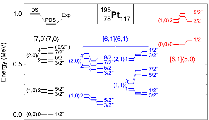
Figure 1: (Color online). Observed and calculated energy spectrum of ¹⁹⁵Pt. The levels in black are the solvable $[7,0]\langle 7,0\rangle$ eigenstates of $\hat{H}_{\rm DS}$ (2), whose structure and energy remain unaffected by the added PDS interactions in Eq. (9). The levels in blue (red) are the $[6,1]\langle 6,1\rangle$ ($[6,1]\langle 5,0\rangle$) eigenstates of $\hat{H}_{\rm DS}$ (2) and are subsequently perturbed by the PDS interactions in Eq. (9). Adapted from isa15 .

The experimental spectrum of ¹⁹⁵Pt is shown in Fig. 1, compared with the DS and PDS calculations. The coefficients $c$, $d$, and $d^{\prime}$ in $\hat{H}_{\rm DS}$ (2) are adjusted to the excitation energies of the $[7,0]\langle 7,0\rangle$ levels which are reproduced with a root-mean-square (rms) deviation of 12 keV. The remaining two coefficients $a$ and $b$ are obtained from an overall fit. The resulting (DS) values are (in keV): $a=45.3$, $b=-41.5$, $c=49.1$, $d=1.7$, and $d^{\prime}=5.6$. The fit for the PDS calculation proceeds in stages. First, the parameters $c$, $d$, and $d^{\prime}$ in Eq. (2) are taken at their DS values. This ensures the same spectrum for the $[7,0]\langle 7,0\rangle$ levels (drawn in black in Fig. 1) which remain eigenstates of $\hat{H}_{\rm PDS}$ (9). Next, one considers the $[6,1]\langle 6,1\rangle$ levels and improves their description by adding the three PDS $U$ interactions. The resulting coefficients are (in keV): $a^{\prime}_{1}=10$, $a_{2}=-97$, and $a_{3}=112$. Eq. (4) ensures that the energies of the $[7,0]\langle 7,0\rangle$ levels do not change while the agreement for the $[6,1]\langle 6,1\rangle$ levels is improved (blue levels in Fig. 1). The rms deviation for both classes of levels is 20 keV. In particular, unlike in the DS calculation, it is possible to reproduce the observed inversion of the $1/2^{-}$-$3/2^{-}$ doublets without changing the order of other doublets. The additional PDS terms necessitate a readjustment of the $a$ coefficient in Eq. (2), for which the final (PDS) value is $a=37.7$ keV, while the coefficient $b$ is kept unchanged. Finally, the position of the $[6,1]\langle 5,0\rangle$ levels (red levels in Fig. 1) is corrected by considering the PDS $V$ interaction with $a_{0}=306$ keV which, due to Eq. (5), has a marginal effect on lower bands. As seen in Fig. 1, the agreement is very good for yrast and non-yrast levels. As shown in Fig. 2, while the states $[7,0]\langle 7,0\rangle$ of the ground band are pure, other eigenstates of $\hat{H}_{\rm PDS}$ in excited bands can have substantial ${\rm SO}^{\rm BF}(6)$ mixing.

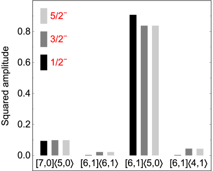
Figure 2: (Color online). ${\rm SO}^{\rm BF}(6)$ decomposition of the eigenstates of $\hat{H}_{\rm PDS}$ (9), shown in red in Fig. 1. Adapted from isa15 .

A large amount of information also exists on electromagnetic transition rates and spectroscopic strengths. In Table 3, 25 measured $B$(E2) values in ¹⁹⁵Pt are compared with the DS and PDS predictions. The same E2 operator is used as in previous studies Bruce85 ; Mauthofer86 of the ${\rm SO}^{\rm BF}(6)$ limit, $\hat{T}_{\mu}({\rm E2})=e_{\rm b}\hat{Q}^{\rm B}_{\mu}+e_{\rm f}\hat{Q}^{\rm F}_{\mu}$, where $\hat{Q}^{\rm B}_{\mu}=s^{\dagger}\tilde{d}_{\mu}+d^{\dagger}_{\mu}s$ is the boson quadrupole operator, $\hat{Q}^{\rm F}_{\mu}=K^{(2)}(2,0)+K^{(2)}(0,2)$ is its fermion analogue (see Table 1), and $e_{\rm b}$ and $e_{\rm f}$ are effective boson and fermion charges, with the values $e_{\rm b}=-e_{\rm f}=0.151$ $e$b. Table 3 is subdivided in four parts according to whether the initial and/or final state in the transition has a DS structure (as in Refs. Bruce85 ; Mauthofer86 ) or whether it is mixed by the PDS interaction. It is seen that when both have a DS structure the $B$(E2) value does not change, only slight differences occur when either the initial or the final state is mixed, and the biggest changes arise when both are mixed.

Table 3: Observed $B({\rm E}2;J_{\rm i}\rightarrow J_{\rm f})$ values between negative-parity states in ¹⁹⁵Pt compared with the DS and PDS predictions of the ${\rm SO}^{\rm BF}(6)$ limit. The solvable (mixed) states are members of the ground (excited) bands shown in Fig. 1. Adapted from isa15 .

${E_{\rm i}}$		$J_{\rm i}$		${E_{\rm f}}$		$J_{\rm f}$		$B({\rm E}2;J_{\rm i}\rightarrow J_{\rm f}$) ($10^{-3}~{}e^{2}{\rm b}^{2}$)
(keV)				(keV)				Exp		DS		PDS
	Solvable $\rightarrow$ solvable
212		${3/2}$		0		${1/2}$		$190(10)$		179		179
239		${5/2}$		0		${1/2}$		$170(10)$		179		179
525		${3/2}$		0		${1/2}$		$17(1)$		0		0
525		${3/2}$		239		${5/2}$		$\leq 19$		72		72
544		${5/2}$		0		${1/2}$		$8(4)$		0		0
612		${7/2}$		212		${3/2}$		$170(70)$		215		215
667		${9/2}$		239		${5/2}$		$200(40)$		239		239
	Solvable $\rightarrow$ mixed
239		${5/2}$		99		${3/2}$		$60(20)$		0		0
525		${3/2}$		99		${3/2}$		$\leq 33$		7		3
525		${3/2}$		130		${5/2}$		$9(5)$		3		2
612		${7/2}$		99		${3/2}$		$5(3)$		9		11
667		${9/2}$		130		${5/2}$		$12(3)$		10		12
	Mixed $\rightarrow$ solvable
99		${3/2}$		0		${1/2}$		$38(6)$		35		34
130		${5/2}$		0		${1/2}$		$66(4)$		35		33
420		${3/2}$		0		${1/2}$		$15(1)$		0		0
456		${5/2}$		0		${1/2}$		$\leq 0.04$		0		0
508		${7/2}$		212		${3/2}$		$55(17)$		20		18
563		${9/2}$		239		${5/2}$		$91(22)$		22		22
199		${3/2}$		0		${1/2}$		$25(2)$		0		0
390		${5/2}$		0		${1/2}$		$7(1)$		0		0
	Mixed $\rightarrow$ mixed
420		${3/2}$		99		${3/2}$		$5(4)$		177		165
508		${7/2}$		99		${3/2}$		$240(50)$		228		263
563		${9/2}$		130		${5/2}$		$240(40)$		253		284
390		${5/2}$		99		${3/2}$		$200(70)$		219		179
390		${5/2}$		130		${5/2}$		$\leq 14$		55		35

V PDS and Intrinsic States

An alternative way of constructing Hamiltonians with PDS for an algebra $G$, is to identify $n$-particle operators which annihilate a lowest-weight state of a prescribed $G$-irrep Alhassid92 . In the IBFM, such a state, which transforms as $[N+1]$ and $\tilde{s}=1/2$ under ${\rm U}^{\rm BF}(6)\otimes{\rm SU}^{\rm F}(2)$, is given by

$$|\Psi_{\rm g}\rangle\propto[b^{{\dagger}}_{c}(\beta)]^{N}f^{{\dagger}}_{\tilde{m}_{s}}(\beta)|0\rangle~{},$$ (10)

where $b^{{\dagger}}_{c}(\beta)\propto(\beta\,d^{{\dagger}}_{0}+s^{{\dagger}})$ and $f^{{\dagger}}_{\tilde{m}_{s}}(\beta)\propto(\beta\,c^{{\dagger}}_{2,0;1/2,\tilde{m}_{s}}+c^{{\dagger}}_{0,0;1/2,\tilde{m}_{s}})$ in the $\tilde{\ell}$-$\tilde{s}$ basis defined above. $|\Psi_{\rm g}\rangle$ is a condensate of $N$ bosons and a single fermion, and represents an intrinsic state for the ground band with deformation $\beta$. The Hermitian conjugate of the following two-particle operators

$${\cal V}^{0(0)}_{+} \propto {\textstyle\sqrt{5}}(d^{\dagger}d^{\dagger})^{(0)}_{0}-{\textstyle\beta^{2}}(s^{\dagger}s^{\dagger})^{(0)}_{0},$$ (11a)

$${\cal V}^{0(1/2)}_{+,\mu} \propto \sqrt{5}(d^{{\dagger}}c^{{\dagger}}_{2;1/2})^{0(1/2)}_{\mu}-\beta^{2}(s^{{\dagger}}c^{{\dagger}}_{0;1/2})^{0(1/2)}_{\mu},\qquad$$ (11b)

$${\cal U}^{{\cal L}({\cal J})}_{+,\mu} \propto (d^{{\dagger}}c^{{\dagger}}_{2;1/2})^{{\cal L}({\cal J})}_{\mu},\quad{\textstyle{\cal L}=1,3},$$ (11c)

$${\cal U}^{2({\cal J})}_{+,\mu} \propto (s^{{\dagger}}c^{{\dagger}}_{2;1/2})^{2({\cal J})}_{\mu}-(d^{{\dagger}}c^{{\dagger}}_{0;1/2})^{2({\cal J})}_{\mu},$$ (11d)

satisfy $\tilde{\cal T}^{{\cal L}({\cal J})}_{-,\mu}|\Psi_{\rm g}\rangle=0$. The $\cal V$ operators of Eqs. (11a)-(11b) satisfy also $\tilde{\cal V}^{0({\cal J})}_{-,\mu}|\Psi_{\rm e}\rangle=0$, where

$$|\Psi_{\rm e}\rangle\propto[b^{{\dagger}}_{c}(\beta)\,c^{{\dagger}}_{2,1;1/2,\tilde{m}_{s}}-d^{{\dagger}}_{1}\,f^{{\dagger}}_{\tilde{m}_{s}}(\beta)][b^{{\dagger}}_{c}(\beta)]^{N-1}|0\rangle$$ (12)

is an intrinsic state, with ${\rm U}^{\rm BF}(6)$ label $[N,1]$, representing an excited band in the odd-mass nucleus. For $\beta=1$, $|\Psi_{\rm g}\rangle$ and $|\Psi_{\rm e}\rangle$ become the lowest-weight states in the ${\rm SO}^{\rm BF}(6)$ irreps $\langle N+1\rangle$ and $\langle N,1\rangle$, respectively, from which the $|(\tau_{1},\tau_{2})LJM_{J}\rangle$ states of Eq. (5) can be obtained by ${\rm SO}^{\rm BF}(5)$ projection, and the operators (11) coincide with those listed in Table 2.

In case of axially-symmetric shapes, SO^BF(5) is no longer a conserved symmetry and the following additional operators can contribute to Hamiltonians with other types of PDS,

$${\cal W}^{{2}(2)}_{+,\mu} \propto \sqrt{2}\beta s^{{\dagger}}d^{{\dagger}}_{\mu}+\sqrt{7}(d^{{\dagger}}d^{{\dagger}})^{(2)}_{\mu},\qquad$$ (13a)

$${\cal W}^{{2}({\cal J})}_{+,\mu} \propto \beta(s^{{\dagger}}c^{{\dagger}}_{2;1/2})^{2({\cal J})}_{\mu}\!+\!\beta(d^{{\dagger}}c^{{\dagger}}_{0;1/2})^{2({\cal J})}_{\mu}\!+\!\sqrt{14}(d^{{\dagger}}c^{{\dagger}}_{2;1/2})^{2({\cal J})}_{\mu}.\;\qquad$$ (13b)

The above operators contain a mixture of components with different ${\rm SO}^{\rm BF}(5)$ character ($\tau=1,2$), and annihilate the intrinsic states of Eqs. (10) and (12). The solvable states are now obtained by angular momentum Spin^BF(3) projection. The operators in Eqs. (11) and (13) are the Bose-Fermi analog of the proton-neutron boson-pair operators comprising the intrinsic part of the IBM-2 Hamiltonian levkir90 , and used in the study of F-spin PDS levgino00 .

VI Summary and Outlook

We have considered an extension of the PDS notion to Bose-Fermi systems and exemplified it in ¹⁹⁵Pt. The analysis highlights the ability of a PDS to select and add to the Hamiltonian, in a controlled fashion, required symmetry-breaking terms, yet retain a good DS for a segment of the spectrum. These virtues greatly enhance the scope of applications of algebraic modeling of complex systems. The operators of Eqs. (11) and (13) can be used to explore additional PDSs in odd-mass nuclei, e.g., SU^BF(3) PDS for $\beta=\sqrt{2}$. Partial supersymmetry, of relevance to nuclei Metz99 , can be studied by embedding ${\rm U}^{\rm B}(6)\otimes{\rm U}^{\rm F}(12)$ in a graded Lie algebra. Work in these directions is in progress.

References

• (1) F. Iachello and A. Arima (1987) The Interacting Boson Model, Cambridge University Press, Cambridge.
• (2) A. Leviatan (2011) Prog. Part. Nucl. Phys. 66 93.
• (3) Y. Alhassid and A. Leviatan (1992) J. Phys. A 25 L1265.
• (4) J. E. García-Ramos, A. Leviatan, and P. Van Isacker (2009) Phys. Rev. Lett. 102 112502.
• (5) A. Leviatan (1996) Phys. Rev. Lett. 77 818.
• (6) A. Leviatan and I. Sinai (1999) Phys. Rev. C 60 061301.
• (7) R. F. Casten, R. B. Cakirli, K. Blaum, and A. Couture (2014) Phys. Rev. Lett. 113 112501.
• (8) A. Couture, R. F. Casten, and R. B. Cakirli (2015) Phys. Rev. C 91 014312.
• (9) A. Leviatan, J. E. García-Ramos, and P. Van Isacker (2013) Phys. Rev. C 87 021302(R).
• (10) A. Leviatan and P. Van Isacker (2002) Phys. Rev. Lett. 89 222501.
• (11) C. Kremer, J. Beller, A. Leviatan, N. Pietralla, G. Rainovski, R. Trippel, and P. Van Isacker (2014) Phys. Rev. C 89 041302(R).
• (12) J. Escher and A. Leviatan (2000) Phys. Rev. Lett. 84 1866.
• (13) J. Escher and A. Leviatan (2002) Phys. Rev. C 65 054309.
• (14) D. J. Rowe and G. Rosensteel (2001) Phys. Rev. Lett. 87 172501.
• (15) G. Rosensteel and D. J. Rowe (2003) Phys. Rev. C 67 014303.
• (16) P. Van Isacker and S. Heinze (2008) Phys. Rev. Lett. 100 052501.
• (17) P. Van Isacker and S. Heinze (2014) Ann. Phys. (N.Y.) 349 73.
• (18) A. Leviatan (2007) Phys. Rev. Lett. 98 242502.
• (19) M. Macek and A. Leviatan (2014) Ann. Phys. (N.Y.) 351 302.
• (20) P. Van Isacker, J. Jolie, T. Thomas and A. Leviatan (2015) Phys. Rev. C 92 011301(R).
• (21) F. Iachello and P. Van Isacker (1991) The Interacting Boson–Fermion Model, Cambridge University Press, Cambridge.
• (22) A. Metz, Y. Eisermann, A. Gollwitzer, R. Hertenberger, B. D. Valnion, G. Graw, and J. Jolie (2000) Phys. Rev. C 61 064313; ibid. (2003) Phys. Rev. C 67 049901(E).
• (23) A. Arima and F. Iachello (1979) Ann. Phys. (N.Y.) 123 468.
• (24) J. A. Cizewski, R. F. Casten, G. J. Smith, M. L. Stelts, W. R. Kane, H. G. Börner, and W. F. Davidson (1978) Phys. Rev. Lett. 40 167.
• (25) P. Van Isacker, A. Frank, and H.-Z. Sun (1984) Ann. Phys. (N.Y.) 157 183.
• (26) R. Bijker and F. Iachello (1985) Ann. Phys. (N.Y.) 161 360.
• (27) A. M. Bruce, W. Gelletly, J. Lukasiak, W. R. Phillips, and D. D. Warner (1985) Phys. Lett. B 165 43.
• (28) A. Mauthofer, K. Stelzer, J. Gerl, Th. W. Elze, Th. Happ, G. Eckert, T. Faestermann, A. Frank, and P. Van Isacker (1986) Phys. Rev. C 34 1958.
• (29) A. Leviatan and M.W. Kirson (1990) Ann. Phys. (N.Y.) 201 13.
• (30) A. Leviatan and J.N. Ginocchio (2000) Phys. Rev. C 61 024305.
• (31) A. Metz, J. Jolie, G. Graw, R. Hertenberger, J. Gröger, C. Günther, N. Warr, and Y. Eisermann (1999) Phys. Rev. Lett. 83 1542.