An effective Hamiltonian approach for Donor-Bridge-Acceptor electronic transitions: Exploring the role of bath memory

Abstract

We present here a formally exact model for electronic transitions between an initial (donor) and final (acceptor) states linked by an intermediate (bridge) state. Our model incorporates a common set of vibrational modes that are coupled to the donor, bridge, and acceptor states and serves as a dissipative bath that destroys quantum coherence between the donor and acceptor. Taking the memory time of the bath as a free parameter, we calculate transition rates for a heuristic 3-state/2 mode Hamiltonian system parameterized to represent the energetics and couplings in a typical organic photovoltaic system. Our results indicate that if the memory time of the bath is of the order of 10–100 fs, a two-state kinetic (i.e., incoherent hopping) model will grossly underestimate overall transition rate.

Key words: super-exchange, electron transfer theory, organic photovoltaics, ultrafast dynamics,
charge transfer

PACS: 87.15.ht, 82.20.Xr, 82.39.Jn

Abstract

Представлено формально точну модель електронних переходiв мiж початковим (донор) та кiнцевим (акцептор) станами, якi зв’язанi промiжним (мiсток) станом. Наша модель включає спiльний набiр коливних мод, якi взаємодiють з донорним, мiстковим та акцепторним станами, та служить як дисипативний термостат, що порушує квантову когерентнiсть мiж донором i акцептором. Беручи час пам’ятi термостата як вiльний параметр, ми розраховуємо iнтенсивнiсть переходiв для евристичного 3-стани/2 модового гамiльтонiана системи, параметризованого для опису енергетики та взаємодiй в типово органiчнiй фотовольтаїчнiй системi. Нашi результати вказують, що якщо час пам’ятi термостату є порядку 10–100 пс, дво-станова кiнетична (тобто з некогерентним перескоком) модель значно недооцiюнює загальну iнтенсивнiсть переходiв.

Ключовi слова: супер-обмiн, теорiя електронного переходу, фотовольтаїка органiчних сполук, надшвидка динамiка, перескок заряду

1 Introduction

In a multi-state system, quantum transitions from an initial to a final state are rarely direct and often involve a coherent transfer between one or more intermediate states. Moreover, for transitions involving the electronic states of molecular systems in which there is significant coupling to a large number of molecular vibrational degrees of freedom, one needs to properly account for the the effects of dissipation, memory, and coherence [1, 2, 3, 4]. This is well known, and a number of methods and approximations with varying degrees of exactness have been developed over the years [5, 6, 7, 8]. Two limits of approximations are the super-exchange model whereby population is transferred from an initial (donor) state to an intermediate state or bridge before being transferred to the final (acceptor) state and the hopping model where population is transferred in a sequence of discrete steps with no quantum coherence between each subsequent step. Reference [9] provides a succinct account of recent progress in this area.

According to the super-exchange model, the electronic coupling between a donor and acceptor linked by $n$ bridging units goes as

$$H_{\text{DA}}=\frac{h_{\text{DB}}}{\Delta\epsilon}\left(\frac{h_{\text{BB}}}{\Delta\epsilon}\right)^{n-1}h_{\text{BA}},$$ (1.1)

where $h_{\text{DB}}$ and $h_{\text{BA}}$ are the electronic (diabatic) couplings between $\text{D}\to\text{B}$ and from $\text{B}\to\text{A}$. The energy gap $\Delta\epsilon$ is the tunneling gap taken as the difference between the $\text{D}\to\text{A}$ transition state and the energy of the bridge-localized states, and $n$ is the number of bridging units with inter-bridge coupling $h_{\text{BB}}$. Given $H_{\text{DA}}$, one can compute the transfer rates using the semi-classical Marcus equation

$$k_{\text{Marcus}}=\frac{2\pi}{\hbar}|H_{\text{DA}}|^{2}\frac{1}{\sqrt{4\pi k_{\text{B}}T\lambda}}\mathrm{e}^{-(\Delta G_{0}+\lambda)^{2}/4\lambda k_{\text{B}}T},$$

where $\Delta G_{0}$ is the driving force and $\lambda$ is the reorganization energy [10, 11, 12]. Considerable amount of work has gone into establishing the validity of the super-exchange model in models of hole-transport in DNA oligomers and electron-transfer dyads linked by $\pi$-conjugated bridges [13, 14, 15, 16, 17, 18, 19].

In a separate context, coherent long-range quantum transport may account for recent observations of ultrafast exciton dissociation in organic polymer: fullerene based photovoltaic systems [20, 21, 22, 23, 24, 25, 1, 2, 26, 27], in artificial light-harvesting systems [28], and natural photosynthetic systems [29]. However, the difficulty using equation (1.1) to compute matrix elements is that the intermediate dynamics within the bridge are completely excluded and it does not account for the fact that the bridge itself may have discrete vibronic states.

In the case of organic photovoltaics, current debate concerns whether or not the charge separation occurs via coherent tunneling or incoherent hopping mechanisms. Pump-push-probe experiments [30, 21] and time-resolved resonant Raman experiments [20] tend to support the notion that that delocalized charge-transfer states are precursors for the formation of charge-separated or polaron states, a view supported by recent theoretical work [4] and others [31, 28]. On the other hand, entropic effects and randomness would lead to localized states and an incoherent hopping mechanism.

With this in mind, we set about to construct a suitable super-exchange theory that accounts for a common vibronic bath coupled to all the electronic states involved in the system and accounts for the fact that the longer the population remains in the bridging state, quantum decoherence will effectively kill the coherent transfer between $\text{D}\to\text{A}$. We also desire a model that can take input directly from a quantum chemical evaluation of the diabatic potentials and electronic couplings for realistic molecular systems [32, 33, 34]. Our approach is similar to that developed recently by Voityuk to study electron transport on molecular wires [35]. As test case, we consider the interstate relaxation dynamics in a model for charge-separation in an organic heterojunction system.

2 Theoretical approach

We consider here a model system consisting of three diabatic electronic states denoted as D, B, and A for ‘‘donor’’, ‘‘bridge’’ and ‘‘acceptor’’ corresponding to the electronic configurations:

$$|\text{D}\rangle=|\text{D}^{*}\cdots\text{B}\cdots\text{A}\rangle,$$ (2.1)

$$|\text{B}\rangle=|\text{D}\cdots\text{B}^{*}\cdots\text{A}\rangle,$$ (2.2)

$$|\text{A}\rangle=|\text{D}\cdots\text{B}\cdots\text{A}^{*}\rangle,$$ (2.3)

where $*$ denotes which of the three electronic states is occupied. The scenario is ubiquitous for charge and energy transfer dynamics and we shall develop our theory without reference to a specific physical process. It suffices to say, D, B, and A are simply different diabatic or localized electronic states of the given physical system. With respect to a common origin, these have energies $E_{\text{D}}$, $E_{\text{B}}$ and $E_{\text{A}}$ respectively. We define a common set of phonon/vibrational modes using boson operators $[a_{q},a_{q^{\prime}}^{\dagger}]=\delta_{qq^{\prime}}$ and frequencies $\omega_{q}$. We shall use these to define diabatic potentials

$$H_{0}=\sum_{n}|n\rangle\langle n|\left\{\left[E_{n}+\sum_{q}g_{nq}(a_{q}^{\dagger}+a_{q})\right]+\sum_{q}\hbar\omega_{q}a_{q}^{\dagger}a_{q}\right\}$$

and off-diagonal electronic couplings

$$V=\sum_{nm}\gamma_{nm}|n\rangle\langle m|$$ (2.5)

that do not depend upon the phonon variables. Note that our linear coupling between the electronic and phonon variables produces a linear displacement in the origins of each electronic potential. Our total Hamiltonian is then the sum $H=H_{0}+V$.

We next want to remove the linear coupling terms by performing a polaron (shift) transformation using

$$\tilde{H}=\mathrm{e}^{-S}H\,\mathrm{e}^{S},$$

where $S$ is an anti-Hermitian operator chosen such that

$$[H_{0},S]=-V.$$

For our purpose at hand, we take

$$S=\sum_{nq}|n\rangle\langle n|\xi_{nq}(a_{q}^{\dagger}-a_{q})$$ (2.6)

and define our transformed operators using the equations of motion method

$$a_{q}(\tau)=\mathrm{e}^{-\tau S}a_{q}\mathrm{e}^{\tau S},$$

where $a_{q}(0)=a_{q}$ and $a_{q}(1)=\tilde{a}_{q}$. This yields

$$a_{q}(\tau)=a(0)-\tau\sum_{n}\xi_{nq}|n\rangle\langle n|.$$

Similarly for $\tilde{a}_{q}^{\dagger}$. Introducing these into $\tilde{H}$, one can diagonalize each term with respect to the phonon variables by setting $\xi_{nq}=g_{nq}/\hbar\omega_{q}$

$$\tilde{H}_{0}=\sum_{n}|n\rangle\langle n|\left(\tilde{E}_{n}+\sum_{q}\hbar\omega_{q}a_{q}^{\dagger}a_{q}\right),$$ (2.7)

where $\tilde{E}_{n}$ is the new energy origin of the $n$th state

$$\tilde{E}_{n}=E_{n}-\sum_{q}\frac{g_{nq}^{2}}{\hbar\omega_{q}}.$$

Similarly, the off-diagonal (diabatic) coupling can be transformed as follows:

$$\tilde{V}=\sum_{nm}\gamma_{nm}|n\rangle\mathrm{e}^{\sum_{q}(\xi_{mq}-\xi_{nq})(a_{q}^{\dagger}-a_{q})}\langle m|.$$

We write the Hamiltonian operator as a $3\times 3$ matrix in the basis of the electronic states:

$$\tilde{H}=\left[\begin{array}[]{ccc}\tilde{H}_{\text{D}}&\tilde{V}_{\text{DB}}&0\\ \tilde{V}_{\text{BD}}&H_{\text{B}}&\tilde{V}_{\text{BA}}\\ 0&\tilde{V}_{\text{AB}}&\tilde{H}_{\text{A}}\end{array}\right].$$ (2.11)

We now seek to eliminate the phonon variables and the explicit description of the bridge electronic state. To this end, we use the Feschbach technique to define the projection operators $\hat{P}=|\text{D}\rangle\langle\text{D}|+|\text{A}\rangle\langle\text{A}|$ and $\hat{Q}=1-\hat{P}=|\text{B}\rangle\langle\text{B}|$ and use these to derive the Green’s function for propagation within the $P$ subspace as influenced by the dynamics within $Q$. First, we write $H_{P}=\hat{P}\tilde{H}\hat{P}$, $H_{Q}=\hat{Q}\tilde{H}\hat{Q}$, and $H_{PQ}=\hat{P}\tilde{H}\hat{Q}$. We then define an effective Hamiltonian by formally solving the Schrödinger equation within the $Q$ subspace and introducing this back into the Schrödinger equation for the $P$ subspace,

$$H_{\textrm{eff}}=H_{P}+H_{PQ}(z-H_{Q})^{-1}H_{QP},$$

where $z$ is the energy taken as a continuous and for now, complex variable. $H_{\text{eff}}$ can be contracted to a $2\times 2$ block matrix with elements

$$H_{\textrm{eff}}=\left[\begin{array}[]{cc}\tilde{H}_{\text{D}}+\Gamma_{\text{DD}}(z)&\Gamma_{\text{DA}}(z)\\ \Gamma_{\text{DA}}^{*}(z)&\tilde{H}_{\text{A}}+\Gamma_{AA}(z)\end{array}\right],$$ (2.14)

where $\Gamma_{ij}(z)$ are the renormalized diabatic couplings:

$$\Gamma_{ij}^{(\pm)}(z)=\tilde{V}_{i\text{B}}\left(z-\tilde{H}_{\text{B}}\pm\mathrm{i}\eta\right)^{-1}\tilde{V}_{\text{B}j},$$ (2.15)

where we have introduced a small $\pm\mathrm{i}\eta$ to insure a proper causality.

2.1 Renormalized couplings

We next derive expressions for these renormalized couplings. To do so, we consider the matrix elements between two vibrational configurations

$$\langle\{n\}|\Gamma_{ij}^{(\pm)}(z)|\{m\}\rangle=\langle\{n\}|\tilde{V}_{i\text{B}}(z-\tilde{H}_{\text{B}}\pm\mathrm{i}\eta)^{-1}\tilde{V}_{\text{B}j}|\{m\}\rangle,$$ (2.16)

where the kets $|\{m\}\rangle$ denote a state in the Fock space specified by the occupation numbers of each mode

$$|\{m\}\rangle=\prod_{q}|m_{q}\rangle.$$

Since the renormalized diabatic couplings do not couple between different phonon modes, we can write these as follows:

$$\langle\{n\}|\Gamma_{ij}^{(\pm)}(z)|\{m\}\rangle=\sum_{q}\langle n_{q}|\Gamma_{ij}^{(\pm)}(z)|m_{q}\rangle$$ (2.17)

and evaluate each term mode by mode

$$\langle n_{q}|\Gamma_{ij}^{(\pm)}(z)|m_{q}\rangle = \langle n_{q}|\tilde{V}_{i\text{B}}(z-\tilde{H}_{\text{B}}\pm\mathrm{i}\eta)^{-1}\tilde{V}_{\text{B}j}|m_{q}\rangle$$ (2.18)

$$= \sum_{l_{q}}\langle n_{q}|\tilde{V}_{i\text{B}}|l_{q}\rangle\langle l_{q}|(z-\tilde{H}_{\text{B}}\pm\mathrm{i}\eta)^{-1}|l_{q}\rangle\langle l_{q}|\tilde{V}_{\text{B}j}|m_{q}\rangle$$

$$= \sum_{l_{q}}\gamma_{i\text{B}}\gamma_{\text{B}j}\langle n_{q}|\exp\big{\{}(\xi_{iq}-\xi_{Bq})(a_{q}^{\dagger}-a_{q})\big{\}}|l_{q}\rangle$$

$$\times\frac{1}{z-(\tilde{E}_{\text{B}}+\hbar\omega_{q}l_{q}\pm\mathrm{i}\eta)}\langle l_{q}|\exp\big{\{}(\xi_{Bq}-\xi_{mq})(a_{q}^{\dagger}-a_{q})\big{\}}|m_{q}\rangle.$$

Define $\Delta\xi_{q}^{ij}=\xi_{iq}-\xi_{jq}$ and write this in terms of the nuclear overlap integrals

$$S_{lmq}^{ij}(\Delta\xi^{ij}_{q})=\langle l_{q}|\exp\big{\{}\Delta\xi^{ij}_{q}(a_{q}^{\dagger}-a_{q})\big{\}}|m_{q}\rangle.$$

These are then used to construct the matrix elements of the couplings

$$\langle n_{q}|\Gamma^{(\pm)}_{ij}(z)|m_{q}\rangle = \sum_{l_{q}}\gamma_{i\text{B}}\gamma_{\text{B}j}\frac{S_{nlq}^{i\text{B}}S_{lmq}^{\text{B}j}}{z-(\tilde{E}_{\text{B}}+\hbar\omega_{q}l_{q})\pm\mathrm{i}\eta}.$$ (2.19)

This last expression can be understood in the following way. An electron from the donor (in vibrational configuration ${\bf m}=\{{\bf m}_{1},{\bf m}_{2},\cdots\}$) is first transferred to the bridging state and the system evolves within the manifold of vibrational states as specified by the nuclear overlap factors between the donor and the bridge. This state then scatters into a specified vibrational of the acceptor state ${\bf n}=\{{\bf n}_{1},{\bf n}_{2},\cdots\}$ with probability dictated by the nuclear overlap between the the bridge and the acceptor. Using the properties of harmonic oscillator states, the overlaps can be evaluated exactly as follows:

$$S_{nl}(\xi) = \frac{1}{\sqrt{n!l!}}\mathrm{e}^{-\xi^{2}/2}\sum_{s=0}^{n}\left(\begin{array}[]{c}n\\ s\end{array}\right)(-\xi)^{n-s}\frac{\mathrm{d}^{s}}{\mathrm{d}\xi^{s}}(\xi^{s}).$$ (2.22)

Note that $\xi$ is related to the relative displacements between the harmonic wells via $\xi=\sqrt{m\omega/\hbar}Q$. In this last expression, we have dropped the explicit reference to the electronic states.

2.2 Perturbation series

To compute the transition probability from the donor to the acceptor states, we construct the Green’s function using the Dyson series:

$$G_{\text{DA}}^{(\pm)}(z)=G_{\text{D}}^{(\pm)}(z)\Gamma_{\text{DA}}^{(\pm)}(z)G_{\text{A}}^{(\pm)}(z)+\cdots$$ (2.23)

which can be written as a sum over all combinations of interaction vertices represented as tadpole diagrams where the loop denotes integration over the vibrational states of the bridge.

(2.24)

where each plain propagator (vertical arrow) is the Green’s function for either the donor or acceptor subspaces ($G_{\text{D}}^{(+)}$ or $G_{\text{A}}^{(+)}$) and the curly line indicates an interaction with the bridge (loop) (i.e., $\Gamma_{\text{DA}}^{(+)}$). To simplify the matters, let us consider the plain propagator as being ‘‘dressed’’ by the interaction with the bridge and include only vertices that scatter from $\text{D}\to\text{A}$ or $\text{A}\to\text{D}$. In essence, we write

$${G}_{\text{D,A}}^{(\pm)}(z)=\frac{1}{z-\big{[}\tilde{H}_{\text{D,A}}+\Gamma_{\text{D,A}}(z)\big{]}\pm\mathrm{i}\eta}$$

as the dressed propagator within the D or A sub-spaces where $\Gamma_{\text{D,A}}(z)$ is the self-energy of the donor or acceptor due to its interaction with the B sub-space. For the off-diagonal terms, the terminal vertices must be ‘‘D’’ for the incoming and ‘‘A’’ for the outgoing terms, implying we have an odd number of interaction vertices. In what follows, we shall neglect the ‘‘diagonal’’ self-energy terms and consider only the first term in the perturbation series.

2.3 Golden rule transition rates

We now use renormalized couplings to compute the transition rates from the donor to the acceptor states. To this end, we recognize that the $\Gamma_{ij}(z)$ vertices are the Fourier-Laplace transforms of Heisenberg operators $\hat{\Gamma}_{ij}(t)$. With this in mind, we can construct time-correlation functions using the Wiener-Khinchin theorem

$${C}_{\text{DA}}(t)=\langle G_{\text{DA}}^{(+)}\star(G_{AD}^{(-)})\rangle,$$

where $\star$ denotes the convolution integral

$${C}_{\text{DA}}(t) = \left\langle\int_{-\infty}^{\infty}\mathrm{d}t\,\;G_{\text{DA}}^{(+)}(z)G_{\text{AD}}^{(-)}(z)\mathrm{e}^{\mathrm{i}zt/\hbar}\right\rangle=\int_{-\infty}^{\infty}\mathrm{d}t\;\mathrm{e}^{\mathrm{i}zt/\hbar}C_{\text{DA}}(z)$$ (2.25)

and $\langle\cdots\rangle$ denotes a sum over both initial and final states, weighted by the populations of the initial states.

$$C_{\text{DA}}(z)=\frac{2\pi}{\hbar}\sum_{q}\sum_{n_{q},m_{q}}\left(\frac{\mathrm{e}^{-\beta\hbar\omega_{q}n_{q}}}{1-\mathrm{e}^{-\beta\hbar\omega_{q}}}\right)|\langle n_{q}|G_{\text{DA}}(z)|m_{q}\rangle|^{2}.$$

(2.26)

Note that the thermal average is a sum over all vibrational modes of the system since we have not distinguished between vibrational modes localized on the donor, bridge, or acceptor units. The golden-rule transition rate can then be determined by evaluating $C_{\text{DA}}(z)$ at the transition energy between the initial and final states, $z=\hbar\omega_{\text{DA}}$.

3 Model calculations

Having derived a relatively compact expression for the golden rule rate between the initial and final electronic states, we can apply this approach to a variety of electronic transitions which are mediated by an intermediate or ‘‘bridge’’ state. In essence, this is a very close to exact expression for the rate of super-exchange between the states in which the electronic transitions are coupled to a manifold of vibrational states. It is important to point out that all the electronic states in our model system are coupled to a common vibronic bath. Hence, our model includes a memory effect that may linger within the vibronic bath over the course of the transition. An important simplification to the model is to partition the vibronic couplings such that the donor, bridge, and acceptor units are coupled to vibrational modes localized on just those units. The model at hand easily allows for this simplification.

As a test case, we consider a 3-electronic state system denoted as $|\text{D}\rangle$, $|\text{B}\rangle$, and $|\text{A}\rangle$ coupled to two independent oscillator modes. We choose our couplings, energetics, and Huang-Rhys parameters according to typical ranges of these values in conjugated organic chromophores and loosely consider the higher frequency vibrational mode to correspond to the in-plane $\text{C}=\text{C}$ stretching modes ($\hbar\omega_{1}=0.15$ eV) and the lower-frequency mode to correspond to the out of plane torsional modes of such molecules ($\hbar\omega_{2}=0.015$ eV) [36, 37, 38, 39]. Table 1 in the appendix gives a summary of the parameters used in our model, and figure 1 shows the adiabatic electronic potentials along the line connecting the local minima of the A and B diabatic potentials. Briefly, we consider the transfer of population from an initially prepared ‘‘donor’’ state with a thermal population of the two vibrational modes.

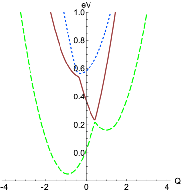
Figure 1: (Color online) Model adiabatic potential curves along the coordinate connecting the bridge and the acceptor minima.

Formally, we introduced $\eta$ in our Greens function to preserve the causality when performing integrations over $z$. $G(z)$ is also a measure of the density of states since each pole represents the energy of a stationary state. For an isolated system, the poles of $G(z)$ become delta-functions in the density of states. However, for a system in contact with a dissipative medium, each delta-function becomes a Lorenzian with an energy width, $\delta E$ and lifetime $\tau$ as governed by the so-called ‘‘time-energy’’ uncertainty relation $\delta E\cdot\tau\geqslant\hbar/2$. Thus, by introducing $\eta$ and shifting the poles off the real-energy axis, we introduce a natural life-time of $\tau\hbar/2\eta$ to each vibrational mode in our model. Consequently, $\eta$ is a free parameter that can be used to characterize the memory effects of the vibronic bath. In essence, making $\eta$ smaller, effectively increases the amount of time the vibronic bath retains the memory of the initial state.

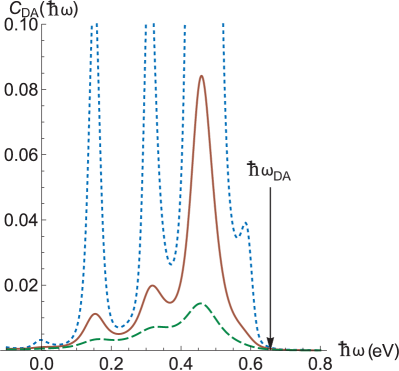
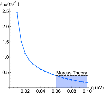
Figure 2: (Color online) (a) Spectral density for $\eta=0.025$ eV (blue), $\eta=0.05$ eV (gold), and $\eta=0.075$ eV (green). The arrow marks the position of the $\text{D}\to\text{A}$ transition frequency between the electronic minima of the D and A adiabatic potential wells. (b) Computed golden-rule rate constants for model system as function of $\eta$.

Figure 2 (a) shows the computed spectral density [equation (2.26)] over a range of values of $\eta$. The peaks correspond to specific energies in which the coupling between the donor and acceptor is strongest, i.e., to resonances within the vibronic bath. Decreasing $\eta$ causes the peaks to become increasingly narrow and more peaked at the resonant frequencies. However, since the golden-rule rate is evaluated at a frequency $\hbar\omega_{\text{DA}}$ that may not be exactly on-resonance with the bath frequency, the changes in the spectral line-shape of the bath have a dramatic impact on the $\text{D}\to\text{A}$ transition rate. In figure 2 (b), we give the computed $\text{D}\to\text{A}$ rates as a function of $\eta$. As expected, the rates decrease as we decrease the memory time of the bath.

As a point of comparison, we consider the extreme case where the $\text{D}\to\text{A}$ transition can be considered as a 3 step process of $\text{D}\to\text{B}\to\text{A}$ with a full loss of coherence (memory) at each step with rate constants given by Marcus theory. Integrating the resulting kinetic equations gives an exact expression

$$p_{A}(t)=1-\frac{k_{2}\mathrm{e}^{-k_{1}t}+k_{1}\mathrm{e}^{-k_{2}t}}{k_{2}-k_{1}}.$$

Taking the half-life of 2 ps to be characteristic of the $\text{D}\to\text{A}$ transition rate, we can make a direct comparison with the DBA rate computed above and estimate a lower limit of $\eta$ for which a two-step (non-superexchange) model would be appropriate. For the case at hand, for $\eta<0.06$ eV, the direct DBA (super-exchange) model predicts the rates faster than the two-step (Marcus) model implying that for cases in which the memory time of the bath is longer than a few 10’s of fs, sequential models of the kinetics will grossly underestimate the transition rates.

We can also approximate the DA coupling using the super-exchange model by taking the energy gap to be the energy difference between where the D and A diabatic curves intersect and the energy minimum of B as $\Delta\epsilon=-0.75$ eV, and one obtains a very small super-exchange coupling of $1.32\times 10^{-4}$ eV and a vanishingly small super-exchange rate of $3.6\times 10^{-7}~{}{\text{fs}}^{-1}$. In this case, the neglect of the vibronic coupling grossly underestimates the rate.

4 Discussion

We have presented here a model for computing the super-exchange transition rates between a model $\text{D}\to\text{B}\to\text{A}$ system composed of 3 electronic states coupled to a common set of vibrational modes. The analysis is generalizable to any number of cases in which there is little to no direct electronic coupling between the initial (D) and the final (A) diabatic states of the system. As a proof of concept, we analyze a simple 3-state/2-mode model parameterized as to represent a prototypical organic photoexcitation system where the relaxation from the initial to the final state proceeds via some common intermediate state. Comparing to a two-step model in which the intermediate rates are determined via Marcus theory, indicates that one needs to be careful in considering the memory effects in the vibrational bath when applying the Marcus theory to a sequence of electronic transitions that occur on the ultra-fast timescale. Our group is currently exploring using the approach delineated in this paper to examine the prompt generation of photocurrent observed in polymer-fullerene based organic photovoltaic cells [20, 4].

Appendix A Model parameters

Table 1: Model parameters for 3-level/2 mode problem.

Description	Symbol	Value
donor energy	$E_{\text{D}}$	0.5 eV
bridge energy	$E_{\text{B}}$	0.55 eV
acceptor energy	$E_{\text{A}}$	0 eV
D-A Diabatic coupling	$\gamma_{\text{DA}}$	$-0.01$ eV
A-B Diabatic coupling	$\gamma_{\text{BA}}$	$-0.01$ eV
Electron Phonon Couplings	$g_{ni}$
donor state	$(g_{\text{D1}},g_{\text{D2}})$	(0, 0)
bridge state	$(g_{\text{B1}},g_{\text{B2}})$	(0.15, 0.06) eV
acceptor state	$(g_{\text{D1}},g_{\text{D3}})$	($-0.15$, $0.01$) eV
Adiabatic minima	$\tilde{E}_{\text{D}}$	0.5 eV
	$\tilde{E}_{\text{B}}$	0.16 eV
	$\tilde{E}_{\text{A}}$	$-0.1567$ eV

Ukrainian 0

Пiдхiд ефективного гамiльтонiану для електронних переходiв донор-мiсток-акцептор: дослiдження
ролi пам’ятi дисипативного середовища Е.Р. Бiттнер

             
Хiмiчний факультет, Унiверситет Г’юстона, Г’юстон, Техас 77204, США

References

-
[1]
Tamura H., Ramon J.G.S., Bittner E.R., Burghardt I.,
Phys. Rev. Lett., 2008, 100, 107402;
doi:10.1103/PhysRevLett.100.107402. - [2] Tamura H., Bittner E.R., Burghardt I., J. Chem. Phys., 2007, 126, 021103; doi:10.1063/1.2431358.
- [3] Pereverzev A., Bittner E.R., J. Chem. Phys., 2006, 125, 104906; doi:10.1063/1.2348869.
- [4] Bittner E.R., Silva C., Nat. Commun., 2014, 5, 3119; doi:10.1038/ncomms4119.
- [5] Stuchebrukhov A., Chem. Phys. Lett., 1994, 225, 55; doi:10.1016/0009-2614(94)00606-7.
- [6] Medvedev E.S., Stuchebrukhov A.A., J. Chem. Phys., 1997, 107, 3821; doi:10.1063/1.474741.
- [7] Scholes G.D., Annu. Rev. Phys. Chem., 2003, 54, 57; doi:10.1146/annurev.physchem.54.011002.103746.
-
[8]
Onuchic J.N., Beratan D.N., Winkler J.R., Gray H.B.,
Annu. Rev. Bioph. Biom., 1992, 21, 349;
doi:10.1146/annurev.bb.21.060192.002025. - [9] Wenger O.S., Acc. Chem. Res., 2011, 44, 25; doi:10.1021/ar100092v.
- [10] Marcus R.A., Sutin N., Biochim. Biophys. Acta, 1985, 811, 265; doi:10.1016/0304-4173(85)90014-X.
- [11] Marcus R.A., J. Chem. Phys., 1965, 43, 679; doi:10.1063/1.1696792.
- [12] Marcus R.A., J. Chem. Phys., 1956, 24, 966; doi:10.1063/1.1742723.
- [13] Lewis F.D., Zhang L., Liu X., Zuo X., Tiede D.M., Long H., Schatz G.C., J. Am. Chem. Soc., 2005, 127, 14445; doi:10.1021/ja0539387.
- [14] Lewis F.D., Photochem. Photobiol., 2005, 81, 65; doi:10.1562/2004-09-01-IR-299.1.
- [15] Starikov E.B., Lewis J.P., Sankey O.F., Int. J. Mod. Phys. B, 2005, 19, 4331; doi:10.1142/S0217979205032802.
- [16] Lewis F.D., Wu Y., Zhang L., Zuo X., Hayes R.T., Wasielewski M.R., J. Am. Chem. Soc., 2004, 126, 8206; doi:10.1021/ja048664m.
- [17] Wang H., Lewis J.P., Stanley O.F., Phys. Rev. Lett., 2004, 93, 016401; doi:10.1103/PhysRevLett.93.016401.
- [18] Lewis F.D., Liu X., Wu H., Zuo X., J. Am. Chem. Soc., 2003, 125, 12729; doi:10.1021/ja036449k.
-
[19]
Lewis J.P., Cheatham Th.E., Starikov E.B., Wang H., Stanley O.F.,
J. Phys. Chem. B, 2003, 107, 2581;
doi:10.1021/jp026772u. - [20] Provencher F., Bérubé N., Parker A.W., Greetham G.M., Towrie M., Hellmann C., Côté M., Stingelin N., Silva C., Hayes S.C., Nat. Commun., 2014, 5, 4288; doi:10.1038/ncomms5288.
- [21] Gélinas S., Rao A., Kumar A., Smith S.L., Chin A.W., Clark J., van der Poll T.S., Bazan G.C., Friend R.H., Science, 2014, 343, 521; doi:10.1126/science.1246249.
- [22] Grancini G., Maiuri M., Fazzi D., Petrozza A., Egelhaaf H.-J., Brida D., Cerullo G., Lanzani G., Nat. Mater., 2013, 12, 29; doi:10.1038/nmat3502.
- [23] Jailaubekov A.E., Willard A.P., Tritsch J.R., Chan W.-L., Sai N., Gearba R., Kaake L.G., Williams K.J., Leung K., Rossky P.J., Zhu X.-Y., Nat. Mater., 2013, 12, 66; doi:10.1038/nmat3500.
- [24] Troisi A., Faraday Discuss., 2013, 163, 377; doi:10.1039/c3fd20142b.
- [25] Lee J., Vandewal K., Yost S.R., Bahlke M.E., Goris L., Baldo M.A., Manca J.V., van Voorhis T., J. Am. Chem. Soc., 2010, 132, 11878; doi:10.1021/ja1045742.
- [26] Bittner E.R., Karabunarliev S., Ye A., J. Chem. Phys., 2005, 122, 034707; doi:10.1063/1.1829032.
- [27] Yang X., Dykstra T.E., Scholes G.D., Phys. Rev. B, 2005, 71, 045203; doi:10.1103/PhysRevB.71.045203.
- [28] Andrea Rozzi C., Falke S.M., Spallanzani N., Rubio A., Molinari E., Brida D., Maiuri M., Cerullo G., Schramm H., Christoffers J., Lienau C., Nat. Commun., 2013, 4, 1602; doi:10.1038/ncomms2603.
- [29] Hayes D., Panitchayangkoon G., Fransted K.A., Caram J.R., Wen J., Freed K.F., Engel G.S., New J. Phys., 2010, 12, 065042; doi:10.1088/1367-2630/12/6/065042.
- [30] Bakulin A.A., Rao A., Pavelyev V.G., van Loosdrecht P.H.M., Pshenichnikov M.S., Niedzialek D., Cornil J., Beljonne D., Friend R.H., Science, 2012, 335, 1340; doi:10.1126/science.1217745.
- [31] Yao Y., Zhou N., Prior J., Zhao Y., Sci. Rep., 2015, 5, 14555; doi:10.1038/srep14555.
- [32] Subotnik J.E., Vura-Weis J., Sodt A.J., Ratner M.A., J. Phys. Chem. A, 2010, 114, 8665; doi:10.1021/jp101235a.
- [33] Yang X., Bittner E.R., J. Chem. Phys., 2015, 142, 244114; doi:10.1063/1.4923191.
- [34] Yang X., Bittner E.R., J. Phys. Chem. A, 2014, 118, 5196; doi:10.1021/jp503041y.
- [35] Voityuk A.A., Phys. Chem. Chem. Phys., 2012, 14, 13789; doi:10.1039/c2cp40579b.
- [36] Karabunarliev S., Bittner E.R., J. Phys. Chem. B, 2004, 108, 10219; doi:10.1021/jp036587w.
- [37] Karabunarliev S., Bittner E.R., J. Chem. Phys., 2003, 118, 4296; doi:10.1063/1.1543938.
- [38] Karabunarliev S., Bittner E.R., Baumgarten M., J. Chem. Phys., 2001, 114, 5863; doi:10.1063/1.1351853.
- [39] Karabunarliev S., Baumgarten M., Bittner E.R., Müllen K., J. Chem. Phys., 2000, 113, 11381; doi:10.1063/1.1328067.
Ukrainian \adddialect\l@ukrainian0 \l@ukrainian