A parametrized non-equilibrium wall-model for large-eddy simulations

ABSTRACT

Wall-models are essential for enabling large-eddy simulations (LESs) of realistic problems at high Reynolds numbers. The present study is focused on approaches that directly model the wall shear stress, specifically on filling the gap between models based on wall-normal ordinary differential equations (ODEs) that assume equilibrium and models based on full partial differential equations (PDEs) that do not. We develop ideas for how to incorporate non-equilibrium effects (most importantly, strong pressure-gradient effects) in the wall-model while still solving only wall-normal ODEs. We test these ideas using two reference databases: an adverse pressure-gradient turbulent boundary-layer and a shock/boundary-layer interaction problem, both of which lead to separation and re-attachment of the turbulent boundary layer.

INTRODUCTION

a)  Test case 1 : STBLI

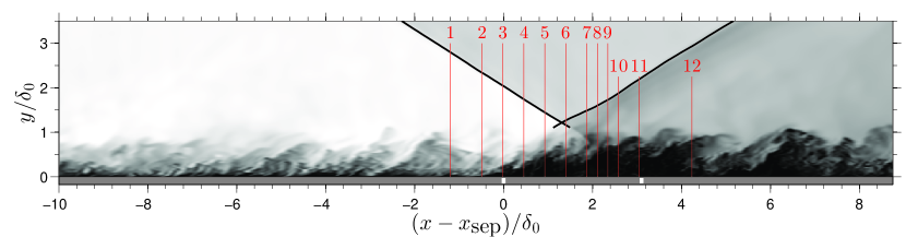
b)  Test case 2 : APGTBL

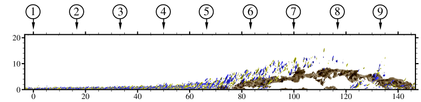
Figure 1: Test cases and interrogation stations used in this study.

1. The 8-degree IUSTI shock/turbulent-boundary-layer interaction (labeled STBLI throughout) experiment of Dupont et al. (2006), with wall-resolved reference LES by Touber & Sandham (2009). Visualization of the instantaneous temperature.

2. The adverse pressure-gradient turbulent boundary-layer (labeled APGTBL throughout) studied in Hickel & Adams (2008). Visualization of the instantaneous coherent structures (Q-criterion) and the separation bubble($u_{1}=0$ iso-surfaces).

Large-eddy simulations (LES) have become part of the basic toolkit for fundamental fluids research. However, the “near-wall problem” of requiring essentially DNS-type grid resolution in the innermost layer of turbulent boundary layers has effectively prevented LES from being applied to many realistic turbulent flows (cf. Piomelli & Balaras, 2002). The solution is to model (rather than resolve) the inner part of turbulent boundary layers, say the innermost 10-20% of the boundary layer thickness $\delta$. By doing this, the grid resolution in an LES is set solely by the need to resolve the remaining outer layer.

There are essentially two different classes of methods that follow this approach. In hybrid LES/RANS and detached eddy simulation (DES), the unsteady evolution equations with an eddy viscosity term are solved everywhere in the domain. The eddy viscosity is then taken from some RANS-type model in the inner layer and some LES-type subgrid model in the outer layer everywhere else in the flow. A second class of methods instead models the wall-stress directly. The LES domain is then defined formally as extending all the way to the wall, while an auxiliary set of equations is solved in an overlapping layer covering the innermost 10-20% of $\delta$. These auxiliary equations are forced by the LES at their upper boundary, and feed the computed wall shear stress and heat transfer back to the LES. The focus in this study is exclusively on the second class of methods.

The most obvious models for the wall stress assume equilibrium; that is, they neglect both the convective and pressure-gradient terms in addition to the wall-parallel diffusive terms. For constant-density flows above the viscous layer, these models yield the famous log-law. While the wall-model only models the innermost 10-20% of $\delta$ (and the LES directly resolves the outermost 80-90%), there has been a long interest in removing the assumption of equilibrium from the wall-model, in hopes of making wall-modeled LES capable of more accurate predictions in the presence of flow separation, etc.

One approach to including non-equilibrium effects was pioneered by Balaras et al. (1996), who solved the thin boundary layer equations (including convection and pressure-gradient, neglecting only wall-parallel diffusion) as a wall-model. From a practical point-of-view, the main drawback of this approach is that a partial differential equation (PDE) must be solved as the wall-model. Thus a full grid with neighbor connectivity is needed in the near-wall layer, in addition to the already existing LES grid. This is a serious obstacle if one seeks to implement the wall-model in an unstructured code for complex geometries. In fact, one could argue that any new wall-model (of the wall-stress kind) will be broadly adopted only if it involves at most connectivity (i.e., derivatives) in the wall-normal direction and time, both of which are easily implemented in a general unstructured code framework.

The challenge, therefore, is to include non-equilibrium effects without the need for wall-parallel derivatives. Hoffmann & Benocci (1995) and Chen et al. (2013) included the pressure-gradient and the temporal term but excluded the convective term. Since the pressure-gradient is constant throughout the wall-modeled layer, and imposed from the LES, this approach does not require wall-parallel derivatives within the wall-model. Wang & Moin (2002) and subsequently Catalano et al. (2003) went one step further and retained only the pressure-gradient term in calculations of the flow over a trailing edge and a circular cylinder, respectively. Neither of these approaches is satisfactory, for reasons to be shown below.

The objective of the present study is to develop a wall-model that includes non-equilibrium effects while still requiring only numerical connectivity in, at most, the wall-normal and temporal directions.

Towards this end, the present paper will:

1. Argue and show that past attempts at including or neglecting the temporal, convective and pressure-gradient terms independently are inconsistent, in the sense that the temporal and convective terms jointly describe the evolution of a fluid particle and that the pressure-gradient and convective terms largely balance outside of the viscous sublayer.

2. Argue and show that the convective term can be parametrized in terms of outer layer LES quantities, thereby eliminating the need for wall-parallel derivatives in the wall-model.

TIME-FILTERED EQUATIONS

When implemented in an LES code, the wall-model is continuously forced by the LES at the upper boundary of the wall-modeled domain (say, at height $h_{\rm wm}$). To give accurate results, $h_{\rm wm}$ should be within the inner part of the boundary layer, so about 10-20% of the boundary layer thickness $\delta$ or less. For accuracy, the grid spacing in the LES needs to be sufficiently small compared to $h_{\rm wm}$ Kawai & Larsson (2012), which implies that $h_{\rm wm}$ should not be chosen too small.

The continuous forcing by the LES at the top boundary means that the wall-model operates in an unsteady mode. The relatively large (RANS-type) eddy viscosity in the wall-model acts as a low-pass filter; therefore, the solution in the wall-modeled layer will be unsteady with primarily low frequencies. This is approximately accounted for in the analysis below by applying a low-pass filter to the wall-resolved LES databases, specifically a top-hat filter with characteristic width $\tau$ defined as

$$\overline{u}(t;\tau)=\frac{1}{\tau}\mathop{\int}_{-\tau/2}^{\tau/2}u(t-t^{\prime})dt^{\prime}\,.$$ (1)

With density-weighting, the associated Favre filter is $\widetilde{u}=\overline{\rho u}/\overline{\rho}$. Application of this filter to the streamwise momentum equation yields to leading order

$$\partial_{t}\widetilde{u}+\widetilde{u}_{j}\partial_{j}\widetilde{u}-\frac{\partial_{2}\left[\mu(\overline{T})\,\partial_{2}\widetilde{u}\right]}{\overline{\rho}}\approx-\frac{\partial_{1}\overline{p}}{\overline{\rho}}-\underbrace{\frac{\partial_{j}(\overline{\rho}\left[\widetilde{u_{j}u}-\widetilde{u}_{j}\widetilde{u}\right])}{\overline{\rho}}}_{\rm modeled}\,,$$ (2)

where wall-parallel diffusion has been neglected, as well as terms due to nonlinearity in the temperature-dependence of the viscosity. The streamwise, wall-normal and spanwise directions (perhaps defined locally) are denoted by subscripts 1, 2 and 3, respectively. For brevity, the streamwise velocity is interchangeably labeled $u$ or $u_{1}$.

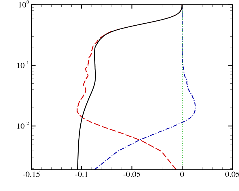
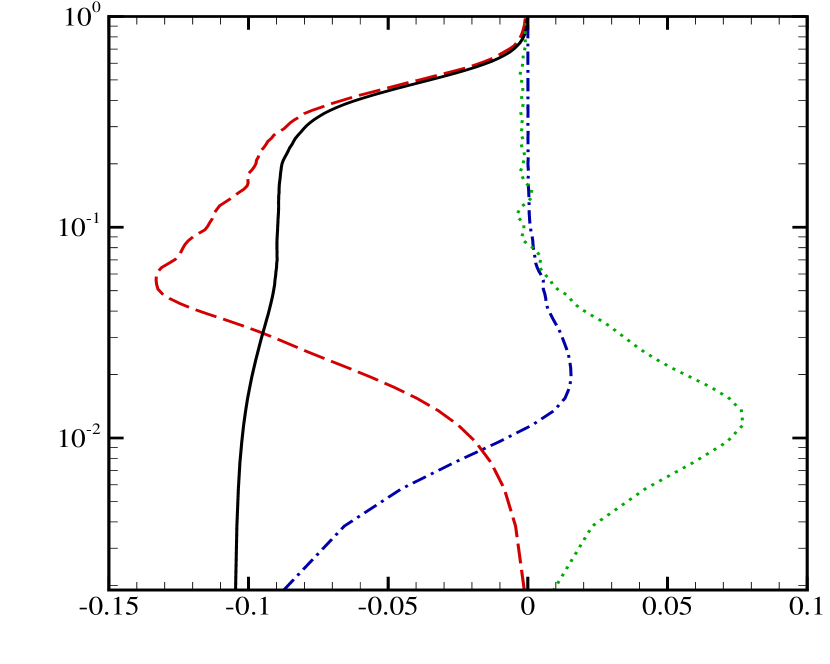
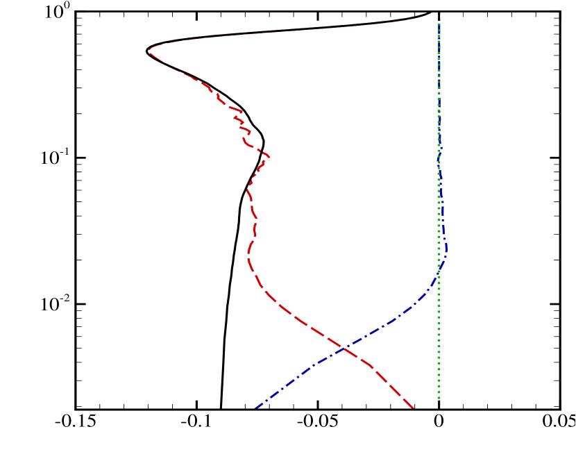
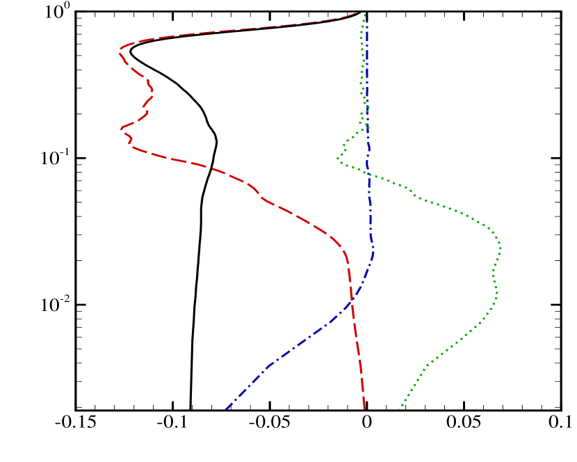
Figure 2: Averaged terms in Eq. (2) for the STBLI case at stations 3 (upper row) and 4 (lower row), filtered using time-scales $\tau U_{\infty}/\delta\approx 0.0$ (left column) and $\tau U_{\infty}/\delta\approx 8.5$ (right column). Pressure-gradient (    ) , viscous term (            ), resolved convection in all three directions (                 ), and unresolved wall-normal Reynolds stress (             ).

TEST CASES

As a first step in this study, data from two reference large-eddy simulations is used to assess the new ideas in an a priori manner. The two reference LESs used sufficiently fine grids to fully resolve the viscous near-wall layer in a quasi-DNS sense.

The first case considered is wall-resolving LES (Touber & Sandham, 2009) of a shock/turbulent-boundary-layer interaction (labeled STBLI throughout) consistent with the flow conditions of the IUSTI experiment of Dupont et al. (2006). An oblique shock wave generated by an 8-degree wedge impinges on a $Ma=2.3$ flat-plate turbulent-boundary layer with a displacement-thickness Reynolds number of $Re_{\delta 1}=21000$. The test case provides regions where equilibrium assumptions are supposed to hold and regions with strong non-equilibrium effects. A visualization of this flow is shown in Figure 1a) based on the instantaneous temperature for the LES of Touber & Sandham (2009).

The second test case is the incompressible non-equilibrium turbulent flat-plate boundary-layer flow of Hickel & Adams (2008) with a displacement-thickness Reynolds number going from $Re_{\delta 1}=1000$ to 30000. Due to the strong non-equilibrium conditions, which result from a constant adverse pressure-gradient imposed at the upper domain boundary, the mean velocity profiles of this boundary layer flow do not follow the classic logarithmic law of the wall. The adverse pressure-gradient decelerates the flow and eventually leads to a highly unsteady and massive flow separation, which is not fixed in space and covers more than a third of the computational domain. The separated flow region and instantaneous coherent structures are visualized in Figure 1b) through an instantaneous iso-surface of $u_{1}=0$ and iso-surfaces of the Q-criterion, respectively. This case is labeled APGTBL throughout this paper.

CONSISTENCY WITH THE
BERNOULLI EQUATION

A typical wall-model essentially solves Eq. (2) with the unresolved convective term parametrized using an eddy viscosity model. The by far most common approach is to assume equilibrium, i.e., to neglect the temporal, resolved convective and pressure-gradient terms. This is exact only for Couette flow, but is a good approximation in many cases.

Hoffmann & Benocci (1995) and, later on, two studies coming out of the Center for Turbulence Research Wang & Moin (2002); Catalano et al. (2003) retained the pressure-gradient term in Eq. (2) but neglected the convective term. One objective of this paper is to point out that this is inconsistent. Consider a flow with a non-zero pressure gradient. In the limit of weak turbulence, for flow in a straight line sufficiently far from the wall such that viscous effects are negligible, Eq. (2) should reduce to the so-called “Euler-s” equation, or, more familiarly (after integration along a streamline), to the Bernoulli equation. In other words, a non-zero pressure-gradient is accompanied by accelerating/decelerating flow, which causes a non-zero streamwise convective term. Therefore, if the pressure-gradient term is explicitly included in the wall-model, then the streamwise convective term must also be included to satisfy this minimal consistency requirement.

Evidence of this is shown in Figures 2 and 3, which show selected terms in the streamwise momentum equation (2) for the two test cases. Results are shown both unfiltered and filtered in time for the first test case, roughly mimicking the effect of the RANS-type eddy viscosity. The filtering hardly affects the viscous and pressure-gradient terms at all, which is to be expected given their essentially linear nature. Note also that not all terms are shown in the figures; thus the sum of all lines is not exactly zero.

The pressure-gradient is essentially balanced by the time-filtered convection term (i.e., the convection that can be resolved by a wall-model) in most of the outer part of the boundary layer, and only within the viscous region does this approximate balance between convection and pressure-gradient break down.

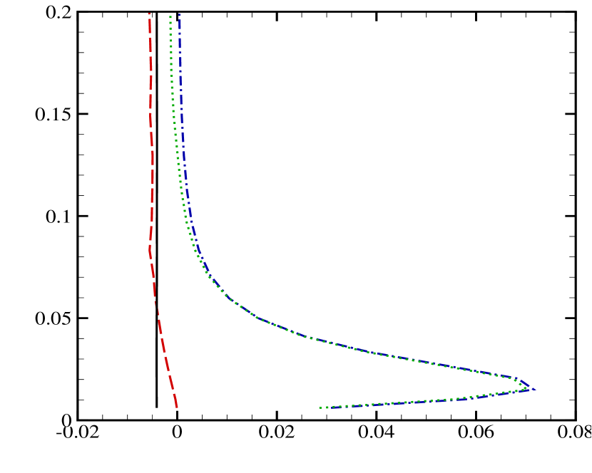
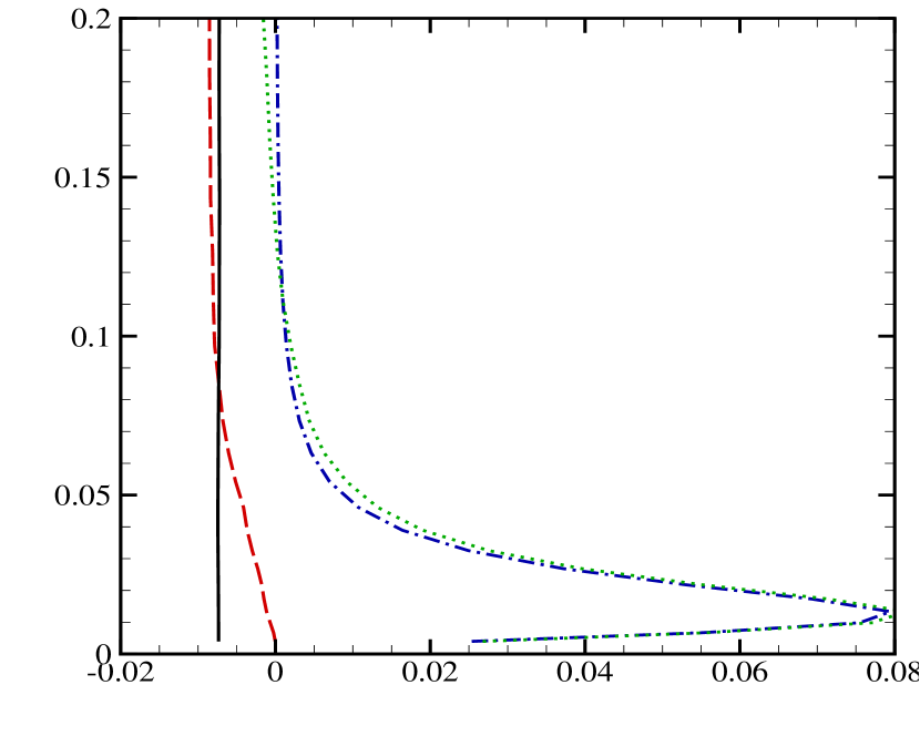
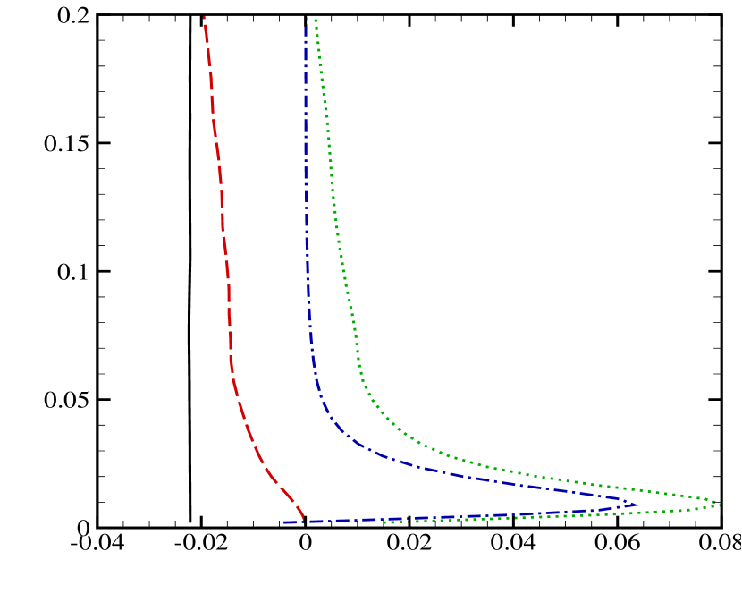
Figure 3: Averaged terms in Eq. (2) for the APGTBL case at stations 1 to 4 using the time-scale $\tau\rightarrow\infty$. Pressure-gradient (    ) , viscous term (            ), resolved convection in all three directions (                 ), and unresolved wall-normal Reynolds stress (             ). All quantities are given in outer scaling, i.e., scaled by the local boundary-layer edge velocity.

CONVECTIVE PARAMETRIZATION

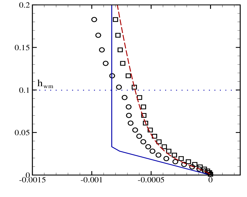
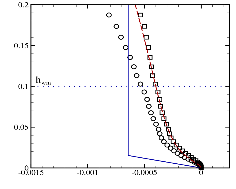
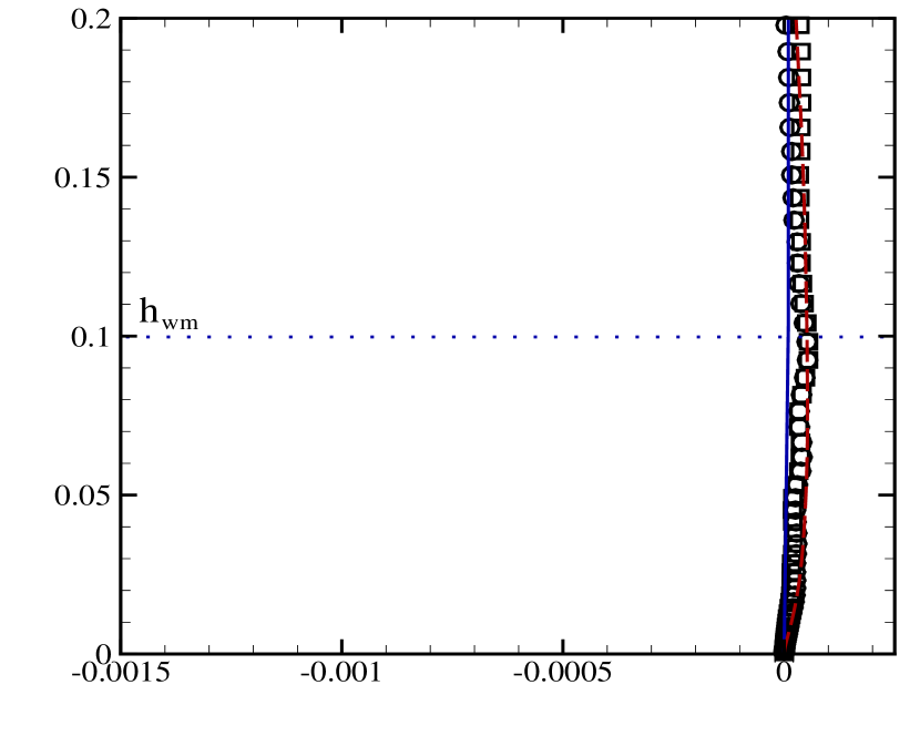
Figure 4: Parametrization of the convective term in terms of the pressure-gradient and velocity profile for the APGTBL case at stations 1, 3, 5 and 8 using the time-scale $\tau\rightarrow\infty$. Approximate $\widetilde{u}_{j}\partial_{j}\widetilde{u}$ from Eq. (3) (    ), Eq. (4) (                 ) , exact $\widetilde{u}\partial_{1}\widetilde{u}$ ($\circ$ ), and exact $\widetilde{u}_{j}\partial_{j}\widetilde{u}$ (        ).

The previous section argued and showed that inclusion of the pressure-gradient term implies that the convective term must also be included for consistency reasons. The convective term, however, includes derivatives in the wall-parallel directions, which implies that a regular grid with full connectivity in all directions is needed to solve the wall-model. While this can be done relatively easily for academic test cases (cf. Balaras et al., 1996; Wang & Moin, 2002; Kawai & Larsson, 2010), it is hard to imagine an implementation in a general-purpose code with an unstructured grid topology. Therefore, it is crucial to remove the need for wall-parallel derivatives in the wall-model.

This can be done by parameterizing the convective term $\widetilde{u}_{j}\partial_{j}\widetilde{u}$ in terms of outer layer quantities, which are available from the LES. The most straight-forward parametrization stems directly from the results shown and discussed in Section CONSISTENCY WITH THE BERNOULLI EQUATION above. Since $\widetilde{u}_{j}\partial_{j}\widetilde{u}$ is essentially balanced by the pressure-gradient $-\partial_{1}\overline{p}/\overline{\rho}$ above the viscous layer, it follows directly that one can approximate

$$\widetilde{u}_{j}\partial_{j}\widetilde{u}\approx-\left.\frac{\partial_{1}\overline{p}}{\overline{\rho}}\right|_{h_{\rm wm}}\cdot\left\{\begin{array}[]{ll}y/y_{\rm pg}&,\ y<y_{\rm pg}\\ 1&,\ y\geq y_{\rm pg}\\ \end{array}\right.$$ (3)

where $y_{\rm pg}$ is the point where viscous effects start damping the streamwise convective term (akin to the thickness of a Stokes layer). For an attached turbulent boundary layer, the value of $y_{\rm pg}$ should be specified in viscous (plus) units for validity across different Reynolds numbers. Since the purpose of this study is to enable wall-models to capture separating flows, we instead set this parameter in viscous pressure-gradient scaling $y_{\rm pg}^{\star}=y_{\rm pg}(\rho_{w}|\partial_{1}p|/\mu_{w}^{2})^{1/3}$; a fixed value of $y_{\rm pg}^{\star}=4$ is used throughout here, with little attempts made at finding an optimal value.

Equation (3) implies that the net effect of convection and pressure-gradient is zero above $y_{\rm pg}$. Thus this parametrization predicts that the logarithmic slope of the mean velocity is independent of the pressure-gradient, but that the additive intercept constant is not (if a regular mixing-length eddy viscosity model is used, such as Eq. (5)).

A second potential parametrization of the convective term is to assume that the streamwise component $\widetilde{u}\partial_{1}\widetilde{u}$ is dominant in the unsteady type of boundary layer flow that occurs in a wall-model, and then to assume that the vertical shape of the derivative $\partial_{1}\widetilde{u}$ can be modeled by the shape of the velocity profile $\widetilde{u}$ itself. In other words, to approximate the convective term as

$$\widetilde{u}_{j}\partial_{j}\widetilde{u}\approx\left|\frac{\widetilde{u}}{\left.\widetilde{u}\right|_{h_{\rm wm}}}\right|^{\alpha}\left.\widetilde{u}_{j}\partial_{j}\widetilde{u}\right|_{h_{\rm wm}}\,,$$ (4)

where the convective term at height $h_{\rm wm}$ is taken from the LES. We found that this approach leads to good predictions that depend only weakly on the precise values of the free parameter $\alpha$; throughout this study $\alpha=3/2$ is used.

These parameterizations of the convective term are tested a priori on the APGTBL case in Figure 4. First, note that the infinite time-filtering for this test case implies that $\widetilde{w}\partial_{3}\widetilde{u}=0$. Secondly, while the $\widetilde{v}\partial_{2}\widetilde{u}$ term is not insignificant, it is small compared to the streamwise component $\widetilde{u}\partial_{1}\widetilde{u}$. The parametrization in terms of velocity, Eq. (4), gives a very reasonable agreement with the wall-resolved LES, while the parametrization in terms of pressure gradient, Eq. (3), only captures the gross features. However, as will be seen below, this is not the complete story.

A PRIORI VALIDATION

To assess the two proposed parameterizations of the convective term, a different type of a priori test is performed. Data from a height $h_{\rm wm}$ above the wall is taken from the wall-resolved reference LES databases and used as the top boundary condition for the wall-model equations; these equations are then solved, and the wall stress is extracted and compared to the actual wall stress in the reference LES databases.

The wall-model is defined by Eq. (2), with the unresolved convective term (the last term) modeled using an eddy-viscosity hypothesis and Eq. (5), and where the sum of the temporal and convective terms (the first two terms) is modeled using either (3) or (4). In the present study, the simple mixing-length model

$$\mu_{t,{\rm wm}}=\kappa\overline{\rho}y\sqrt{\frac{\widetilde{\tau}_{w}}{\overline{\rho}}}\left[1-\exp\left(\frac{-y^{+}}{A^{+}}\right)\right]^{2}\,,$$ (5)

with $\kappa=0.41$ and $A^{+}=17$ is used.

A finite volume approach is used to discretize the equations, and convergence is achieved using a Newton-type iterative procedure. Identical formulations are used for both databases with identical parameters, and compared with an equilibrium wall-model as well as the non-equilibrium wall-model of Duprat et al. (2011).

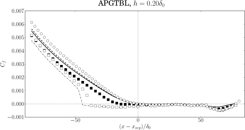
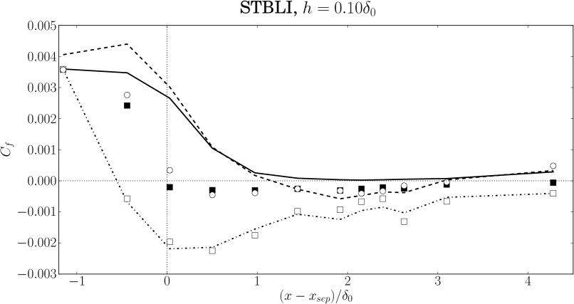
Figure 5: A-priori study: Friction coefficient obtained using various non-equilibrium formulations and compared to existing models. Exact from reference LES ($\circ$ ), equilibrium model (    ), model of Duprat et al. (2011) (                 ), adding $\partial_{1}p$ by itself (            ), adding $\partial_{1}p$ + Eq. (3) with $(y_{pg}^{*}=4)$ (  ), adding $\partial_{1}p$ + Eq. (4) (        ).

The results are shown in Figure 5. In the APGTBL case, all of the different wall-models under-predict the skin friction; this could be due to the low Reynolds number in this case ($Re_{\tau}\approx 400$ at station 1), for which the wall-model parameters are not optimal.

If the pressure-gradient is included without any additional modeling (as done by Hoffmann & Benocci, 1995; Wang & Moin, 2002; Catalano et al., 2003; Chen et al., 2013), the skin friction is further under-predicted, and separation occurs much too early.

Including both the pressure-gradient and a parametrized convective term gives a model which satisfies the necessary “Bernoulli consistency.” Despite this, and despite producing impressive a priori agreement of the vertical profiles in Fig. 4, the parametrization based on the velocity profile, Eq. (4), gives disappointing results, hardly better than without the convective term at all. In contrast, the parametrization based on the pressure-gradient, Eq. (3), gives excellent results for the STBLI case and reasonable results for the APGTBL case, albeit a bit worse than the results of the basic equilibrium model. We also note that the parametrization based on the velocity profile is more sensitive to numerical convergence issues, while the parametrization based on the pressure-gradient was found to be numerically robust.

The model of Duprat et al. (2011) gives disappointing results, essentially no different from the basic equilibrium model for the APGTBL case and with severely over-predicted wall shear for the STBLI case.

SUMMARY

Wall-models are essential for enabling the use of large-eddy simulations on realistic problems at high Reynolds numbers. The present study is focused on approaches that directly model the wall shear stress, specifically on filling the gap between models based on wall-normal ODEs that assume equilibrium and models based on full PDEs that do not. Ideas for how to incorporate non-equilibrium effects (most importantly, strong pressure-gradient effects) in the wall-model while still solving only wall-normal ODEs are developed and tested using two reference databases computed using wall-resolved LES: an adverse pressure-gradient turbulent boundary-layer and a shock/boundary-layer interaction problem, both of which lead to boundary-layer separation and re-attachment.

First, it is pointed out that the convective term and the pressure-gradient term must be treated consistently with each other, since a non-zero pressure-gradient is almost necessarily associated with a non-zero convective acceleration; these terms will have offsetting contributions in most cases. The bottom line is that these terms should either be retained or neglected jointly, not independently as done in several prior studies (e.g., Hoffmann & Benocci, 1995; Wang & Moin, 2002; Catalano et al., 2003). Similarly, since the temporal and convective terms jointly describe the acceleration of a fluid particle in its Lagrangian frame, for consistency these two terms must be treated in the same way as well.

Next, it is argued that a non-equilibrium wall-model in ODE-form requires that the convective terms be parametrized using LES data from the top of the wall-modeled layer. Two forms of this parametrization are proposed: one based on the pressure-gradient, one based on the velocity profile and the LES velocity gradient. When assessed a priori using the reference databases, no clear conclusion is reached: the pressure-based parametrization can capture only the gross features of the convective term, whereas the second parametrization based on the velocity profile gives a very good agreement with the wall-resolved LES data. However, when used to compute the skin friction in the two test cases, the model based on the pressure-gradient appears superior: the predicted skin friction is very close to the reference one for the shock/boundary-layer interaction case, but slightly under-predicted for the adverse pressure-gradient case.

References

- Balaras et al. (1996) Balaras, E., Benocci, C. & Piomelli, U. 1996 Two-layer approximate boundary conditions for large-eddy simulations. AIAA J. 34 (6), 1111–1119.
- Catalano et al. (2003) Catalano, P., Wang, M., Iaccarino, G. & Moin, P. 2003 Numerical simulation of the flow around a circular cylinder at high reynolds numbers. Int. J. Heat Fluid Flow 24, 463–469.
- Chen et al. (2013) Chen, Z. L., Hickel, S., Devesa, A., Berland, J. & Adams, N. A. 2013 Wall modeling for implicit large-eddy simulation and immersed-interface methods. Theor. Comput. Fluid Dyn., DOI: 10.1007/s00162-012-0286-6.
- Dupont et al. (2006) Dupont, P., Haddad, C. & Debieve, J. F. 2006 Space and time organization in a shock-induced separated boundary layer. J. Fluid Mech. 559, 255–277.
- Duprat et al. (2011) Duprat, C., Balarac, G., Metais, O., Congedo, P. M. & Brugiere, O. 2011 A wall-layer model for large-eddy simulations of turbulent flows with/out pressure gradient. Phys. Fluids 23, 015101.
- Hickel & Adams (2008) Hickel, S. & Adams, N. A. 2008 Implicit LES applied to zero-pressure-gradient and adverse-pressure-gradient boundary-layer turbulence. Int. J. Heat Fluid Flow 29, 626–639.
- Hoffmann & Benocci (1995) Hoffmann, G. & Benocci, C. 1995 Approximate wall boundary conditions for large eddy simulations. In Advances in turbulence V: Proceedings of the 5th European Turbulence Conference, 222–228.
- Kawai & Larsson (2010) Kawai, S. & Larsson, J. 2013 Dynamic non-equilibrium wall-modeling for large eddy simulation at high Reynolds numbers. Phys. Fluids 25, 015105.
- Kawai & Larsson (2012) Kawai, S. & Larsson, J. 2012 Wall-modeling in large eddy simulation: length scales, grid resolution and accuracy. Phys. Fluids 24, 015104.
- Piomelli & Balaras (2002) Piomelli, U. & Balaras, E. 2002 Wall-layer models for large-eddy simulations. Annu. Rev. Fluid Mech. 34, 349–374.
- Touber & Sandham (2009) Touber, E. & Sandham, N. 2009 Large-eddy simulation of low-frequency unsteadiness in a turbulent shock-induced separation bubble. Theor. Comp. Fluid Dyn. 23, 79–107.
- Wang & Moin (2002) Wang, M. & Moin, P. 2002 Dynamic wall modeling for large-eddy simulation of complex turbulent flows. Phys. Fluids 14 (7), 2043–2051.