Generalized isotropic Lipkin–Meshkov–Glick models: ground state entanglement and quantum entropies

Abstract

We introduce a new class of generalized isotropic Lipkin–Meshkov–Glick models with $\mathrm{su}(m+1)$ spin and long-range non-constant interactions, whose non-degenerate ground state is a Dicke state of $\mathrm{su}(m+1)$ type. We evaluate in closed form the reduced density matrix of a block of $L$ spins when the whole system is in its ground state, and study the corresponding von Neumann and Rényi entanglement entropies in the thermodynamic limit. We show that both of these entropies scale as $a\log L$ when $L$ tends to infinity, where the coefficient $a$ is equal to $(m-k)/2$ in the ground state phase with $k$ vanishing $\mathrm{su}(m+1)$ magnon densities. In particular, our results show that none of these generalized Lipkin–Meshkov–Glick models are critical, since when $L\to\infty$ their Rényi entropy $R_{q}$ becomes independent of the parameter $q$. We have also computed the Tsallis entanglement entropy of the ground state of these generalized $\mathrm{su}(m+1)$ Lipkin–Meshkov–Glick models, finding that it can be made extensive by an appropriate choice of its parameter only when $m-k\geqslant 3$. Finally, in the $\mathrm{su}(3)$ case we construct in detail the phase diagram of the ground state in parameter space, showing that it is determined in a simple way by the weights of the fundamental representation of $\mathrm{su}(3)$. This is also true in the $\mathrm{su}(m+1)$ case; for instance, we prove that the region for which all the magnon densities are non-vanishing is an $(m+1)$-simplex in ${\mathbb{R}}^{m}$ whose vertices are the weights of the fundamental representation of $\mathrm{su}(m+1)$.

Keywords: entanglement in extended quantum systems (theory), solvable lattice models, conformal field theory (theory)

1 Introduction

A crucial difference between classical and quantum systems is the fact that in the latter ones the entropy of a subsystem can be positive even when the whole system is in its (pure) ground state at zero temperature. Indeed, classically a positive value of the entropy is simply a reflection of the lack of knowledge of the precise microstate of the system when it is in a certain macrostate. On the other hand, an essential property of quantum systems is the fact that the exact knowledge of the state of the whole system does not give complete information about the state of a subsystem. This is a consequence of the entanglement among different parts of the system, which is perhaps the most paradigmatic quantum phenomenon [1, 2].

One of the most widespread quantitative measures of the degree of entanglement of a quantum system at zero temperature is the bipartite entropy of its ground state $|\psi\rangle$. More precisely, if we divide the system into two subsystems with $L$ and $N-L$ particles the corresponding bipartite entropy is the quantum entropy of the reduced density matrix $\rho_{L}=\tr_{N-L}\rho$, where $\rho\equiv|\psi\rangle\langle\psi|$ and the trace is taken over the degrees of freedom of the latter subsystem. This definition is actually symmetric between both subsystems, since the entropy of $\rho_{L}$ necessarily coincides with that of $\rho_{N-L}$. In practice, the von Neumann [1] and Rényi [3, 4] entropies, respectively defined by

$$S=-\tr(\rho_{L}\log\rho_{L}),\qquad R_{q}=\frac{\log\tr(\rho_{L}^{q})}{1-q}$$ (1.1)

(where $q$ is a positive real parameter) have been extensively used as quantitative measures of the bipartite entanglement. The exact evaluation of these entropies, or even the determination of their large $L$ limit, is only possible for a handful of mostly one-dimensional models. These models include the XX and XY nearest-neighbors Heisenberg spin chains, for which the asymptotic behavior of both the von Neumann and Rényi entropies was established in the last decade [5, 6, 7] with the help of the Fisher–Hartwig conjecture. As is well known, both of these models are critical in a certain region of their parameter space [8]. The large $L$ behavior of the entropy is essentially different in the critical and non-critical regions. More precisely, the entropy scales as $\log L$ in the critical region, while it saturates to a constant in the non-critical one. This is a manifestation of the so-called area law [9], according to which the (von Neumann) bipartite entropy of a critical one-dimensional quantum system with short-range interactions behaves as $\log L$, while for non-critical systems it tends to a constant. This is consistent with the fact that the bipartite entropy of two-dimensional conformal field theories (which describe one-dimensional quantum critical systems in the thermodynamic limit) scales as $(c+\bar{c})(1+q^{-1})(\log L)/12$, where $c$ and $\bar{c}$ denote respectively the holomorphic and anti-holomorphic central charges and $q=1$ for the von Neumann entropy [10, 11, 12].

On the other hand, it is generally believed that the area law need not hold for systems exhibiting long-range interactions, since the stronger correlations in these systems are expected to increase the entropy. One of the few one-dimensional long-range quantum systems that has been exactly solved is the Lipkin–Meshkov–Glick (LMG) model [13, 14, 15], originally introduced by the latter authors to describe a system of $N$ fermions in two levels each of which is $N$ times degenerate. This model is equivalent to a system of $N$ spin $1/2$ particles with constant XY-type long-range interactions in a transverse magnetic field. In the isotropic (XX) case the model is exactly solvable, and its bipartite von Neumann entropy has also been computed in closed form [16, 17]. The von Neumann entropy vanishes in the gapped (and not entangled) phase, while it grows as $(\log L)/2$ in the gapless one. Thus the LMG model behaves in this respect as a one-dimensional quantum system with short-range interactions. The reason of this behavior is the competition between the range of the interactions, which tends to increase the entropy, and the high degree of symmetry of this model, which tends to lower it. Indeed, in this case the ground state is a symmetric Dicke state (i.e., it has maximum total spin $S=N/2$ and a well-defined value of the total spin component $S^{z}$) for all values of its parameters, which is easily seen to imply that the entanglement entropy cannot exceed $\log(L+1)$.

A class of one-dimensional models with long-range interactions which has been extensively studied is that of spin chains of Haldane–Shastry (HS) type. The original HS chain [18, 19] is a lattice model of $N$ spin $1/2$ particles uniformly arranged on a circle, with pairwise interactions inversely proportional to the square of the chord distance. This model was soon afterwards generalized to particles carrying $\mathrm{su}(m+1)$ spin, as well as to rational and hyperbolic interactions [20, 21, 22, 23]. The HS chain, which is closely related to the one-dimensional Hubbard model with long-range hopping [24], is exactly solvable via the asymptotic Bethe ansatz, and its partition function can be evaluated in closed form [25]. Among other remarkable properties, the HS chain possesses exact Yangian symmetry for a finite number of sites [26], and provides one of the simplest realizations of anyons in one dimension via Haldane’s fractional statistics [27, 26, 28, 29].

In this paper we shall introduce a large family of $\mathrm{su}(m+1)$ spin chains which, like the HS-type chains, feature variable long-range interactions, and whose ground state entanglement properties are similar to those of the isotropic LMG model. More precisely, the models we shall construct will admit as non-degenerate ground state a generalized Dicke state of $\mathrm{su}(m+1)$ type, i.e., a state totally symmetric under permutations and with a well defined number of particles in each of the $\mathrm{su}(m+1)$ internal one-particle states ($\mathrm{su}(m+1)$ magnons). This will be achieved by replacing the quadratic term in the total spin operator $S^{z}$ present in the LMG Hamiltonian by a sum of similar terms in each of the generators of the $\mathrm{su}(m+1)$ Cartan subalgebra. The resulting models can thus be considered a natural generalization of the original (isotropic) LMG model, to which they actually reduce when $m=1$ and all the two-body interactions are constant.

An explicit expression for the reduced density matrix $\rho_{L}$ of any system whose ground state is an $\mathrm{su}(m+1)$-type Dicke state with arbitrary $m$ first appeared in Ref. [30]. The eigenvalues of $\rho_{L}$ turn out to define a hypergeometric distribution in $m$ variables, thus generalizing the result of Refs. [16, 17] for the spin $1/2$ ($m=1$) isotropic LMG model. We shall show that in the thermodynamic limit $N\gg 1$ with $L/N\to\alpha$ (finite) the eigenvalues of the reduced density matrix can be well approximated by a Gaussian distribution, whose parameters we evaluate in closed form for arbitrary $m$ and $\alpha$. With the help of this approximation, we obtain explicit asymptotic expressions for the von Neumann and Rényi entropies in the thermodynamic limit. In particular, our expression for the von Neumann entropy coincides with that of Ref. [30], derived by extrapolation from the $\alpha=0$ case. Remarkably, in the region of parameter space for which all the ground state magnon densities are non-vanishing both of these entropies scale as $(m\log L)/2$ as $L$ tends to infinity. Thus the behavior of the von Neumann entropy is that of a critical model with $c=\bar{c}=3m/2$, described by a conformal field theory (CFT) with $m$ fermions and $m$ bosons. This may not seem surprising at first sight, taking into account that many critical one-dimensional spin chains, including the Heisenberg (XXX) and the $\mathrm{su}(m+1)$ HS chains, are effectively described by theories of this type (see, e.g., [26, 31, 32]). Here, however, the situation is more subtle. Indeed, the Rényi entropy $R_{q}$, although still proportional to $\log L$ for large $L$, becomes independent of the parameter $q$ for $L\to\infty$, and as a consequence the family of generalized isotropic LMG models cannot contain any critical instances.

It is well known that a crucial requirement of classical thermodynamics is the extensivity of the (Maxwell–Boltzmann) entropy of a given system, i.e., that $S\propto L^{d}$, where $L$ is a characteristic length of the system and $d$ is the number of space dimensions. In a quantum context this requirement, at least for the von Neumann entropy, is violated in many cases, as for instance in black hole thermodynamics [33, 34, 35, 36]. In fact, the area law mentioned above evidences a non-extensive behavior of von Neumann’s entropy in strongly correlated quantum systems. On the other hand, it is very natural to enquire whether this feature is shared by all quantum entropies available in the literature. Interestingly enough, this is not the case. For instance, as already noted in Ref. [37], the quantum Tsallis entropy [38, 39] can be extensive when von Neumann’s is not in several one- and two-dimensional strongly correlated systems, which include the Heisenberg XY model. We have found a similar behavior for the Tsallis entanglement entropy of the ground state of generalized $\mathrm{su}(m+1)$ LMG models with $m-k\geqslant 3$ (where $k$ is the number of vanishing magnon densities), while for $m-k=1,2$ the Tsallis entropy is not extensive for any value of its parameter.

As mentioned above, the ground state of the isotropic LMG model has two quantum phases (entangled and non-entangled), respectively determined by the values of the (suitably normalized) magnetic field strength being less or greater than $1$ in absolute value. For the generalized LMG models constructed in this paper, the situation is more subtle. More precisely, we shall show that in this case the ground state can be in exactly $m+1$ quantum phases, each of which is characterized by the vanishing of a certain number of magnon densities. Moreover, in the phase with $k$ vanishing magnon densities both the von Neumann and Rényi entropies scale as $\frac{1}{2}(m-k)\log L$, implying again that none of these phases can contain any critical models. We have performed a detailed analysis of the ground state phases in the $\mathrm{su}(3)$ ($m=2$) case, completely identifying the corresponding regions in parameter space. Remarkably, these regions are entirely determined in a geometric way by the weights of the fundamental representation of $\mathrm{su}(3)$ associated to the choice of the Cartan generators. A similar result holds in the general ($\mathrm{su}(m+1)$) case; for instance, we show that the region for which all the magnon densities are non-vanishing is an $(m+1)$-simplex in ${\mathbb{R}}^{m}$ whose vertices are the weights of the fundamental representation of $\mathrm{su}(m+1)$.

We end this section with a few words on the paper’s organization. In Section 2 we review the main properties of the isotropic LMG model and present the construction of its $\mathrm{su}(m+1)$ generalization with non-constant interactions. In Section 3 we evaluate in closed form the ground state entanglement entropies of von Neumann and Rényi, and study their main properties. As a byproduct of our analysis, we obtain a similar expression for the Tsallis entropy and discuss its extensivity. In Section 4, a detailed description of the entanglement properties of the ground state as a function of the $\mathrm{su}(m+1)$ magnetic field strength is presented. Special attention is paid to the case $m=2$, for which we obtain a complete phase diagram describing the regions in parameter space with different magnon content. Section 5 is devoted to the presentation of our conclusions and the discussion of some open problems suggested by the previous results. The paper ends with three technical appendices in which we present a detailed derivation of the exact formula for the eigenvalues of the reduced density matrix, compute the first and second moments of a multivariate hypergeometric distribution, and show how a univariate hypergeometric distribution can be approximated by a normal one in a suitable limit.

2 Generalized Lipkin–Meshkov–Glick models

The original Lipkin–Meshkov–Glick model describes a system of $N$ mutually interacting spin 1/2 particles in a constant magnetic field. Its Hamiltonian can be taken as

$$H=-\frac{\lambda}{N}\sum_{i<j}\left(\sigma^{x}_{i}\sigma^{x}_{j}+\gamma\sigma^{y}_{i}\sigma^{y}_{j}\right)-h\sum_{i}\sigma^{z}_{i},$$ (2.1)

where $\lambda>0$, $\gamma\geqslant 0$ and $h$ are real parameters, $\sigma^{a}_{k}$ is the $a$-th Pauli matrix acting on the $k$-th spin, and the sums (as hereafter, unless otherwise stated) range from $1$ to $N$. The model (2.1) is thus the analogue of the Heisenberg XY chain with long-range constant interactions. Its Hamiltonian can be expressed in terms of the total spin operators $S^{a}=\sum_{i}\sigma^{a}_{i}/2$ as

$$H=-\frac{\lambda}{N}(1+\gamma)\Big{(}\mathbf{S}^{2}-(S^{z})^{2}-{\textstyle\frac{N}{2}}\Big{)}-2hS^{z}-\frac{\lambda}{2N}(1-\gamma)\Big{(}(S^{+})^{2}+(S^{-})^{2}\Big{)},$$ (2.2)

where $\mathbf{S}=(S^{x},S^{y},S^{z})$ and $S^{\pm}=S^{x}\pm\rmi S^{y}$.

It is well known [40, 41] that the LMG model undergoes a second-order quantum phase transition with mean field exponents at $h/\lambda=1$. In the anisotropic case $0\leqslant\gamma<1$, the model has been solved only in the thermodynamic limit [42, 43], although its entanglement properties have been extensively studied (see, e.g., [44, 45, 46]). In this work we shall focus on the isotropic case $\gamma=1$, for which $H$ is diagonal in a basis $|S,M,\nu\rangle$ of common eigenstates of $\mathbf{S}^{2}$ and $S^{z}$ with respective eigenvalues $S(S+1)$ and $M$. Here, as usual, $M=-S,-S+1,\dots,S$ and $S=\pi(N)/2,\pi(N)/2+1,\dots,N/2$, where $\pi(N)$ denotes the parity of the integer $N$. We shall further set $\lambda=1$ (which amounts to a trivial rescaling) and also restrict ourselves, without loss of generality, to nonnegative values of $h$ (since the spectrum of $H$ is clearly independent of the sign of $h$). With this choice of parameters Eq. (2.2) implies that $H|S,M,\nu\rangle=E(S,M)|S,M,\nu\rangle$, where the eigenvalue $E(S,M)$ is given by

$$E(S,M) =-\frac{2}{N}\Big{(}S(S+1)-M^{2}-N/2\Big{)}-2hM$$ (2.3)

$$=-\frac{2}{N}\,S(S+1)+\frac{2}{N}\left(M-\frac{Nh}{2}\right)^{2}-\frac{Nh^{2}}{2}+1\,.$$

The properties of the ground state of the LMG model (2.1) with $\lambda=\gamma=1$ and $h\geqslant 0$ are essentially different in the two quantum phases $0\leqslant h<1$ and $h\geqslant 1$. Indeed, for $h\geqslant 1$ the minimum of Eq. (2.3) is achieved when $S=M=N/2$, so that the ground state is the product state with all spins up. In particular, for $h\geqslant 1$ the ground state is not entangled. On the other hand, when $0\leqslant h<1$ the energy is clearly a minimum when $S=N/2$ and $M=I(hN/2)$, where $I(x)$ denotes the closest integer (for $N$ even) or half-integer (for $N$ odd) to $x$. In particular, since the total spin $S$ is maximum the ground state must be totally symmetric. It is also non-degenerate, since the number $N_{\uparrow}$ of “up” spins is fixed by the condition

$$M=I(hN/2)=\frac{1}{2}\,(N_{\uparrow}-N_{\downarrow})=N_{\uparrow}-\frac{N}{2}\enspace\Longrightarrow\enspace N_{\uparrow}=\frac{N}{2}+I(hN/2)\,,$$ (2.4)

where $N_{\downarrow}=N-N_{\uparrow}$ denotes the number of “down” spins. Thus, when $0\leqslant h<1$ the ground state of the LMG Hamiltonian (2.1) with $\gamma=\lambda=1$ is the totally symmetric state

$$|\psi(N_{\uparrow},N_{\downarrow})\rangle\equiv|N/2,I(hN/2)\rangle\,,$$ (2.5)

where $N_{\uparrow}$ is given by (2.4). Denoting by $|\!\!\uparrow\rangle$ and $|\!\!\downarrow\rangle$ respectively the spin up and down one-particle states, the (normalized) ground state (2.5) can be expressed in terms of the elements

$$|s_{1},\dots,s_{N}\rangle\equiv|s_{1}\rangle\cdots|s_{N}\rangle\equiv|s_{1}\rangle\otimes\cdots\otimes|s_{N}\rangle\,,\qquad s_{k}=\uparrow,\downarrow\,,$$

of the canonical spin basis as

$$|\psi(N_{\uparrow},N_{\downarrow})\rangle={N\choose N_{\uparrow}}^{-\frac{1}{2}}\sum_{p\in S_{N_{\uparrow},N_{\downarrow}}}|p(\underbrace{\uparrow,\dots,\uparrow,}_{N_{\uparrow}}\underbrace{\downarrow,\dots,\downarrow}_{N_{\downarrow}})\rangle\,.$$ (2.6)

In the latter formula $S_{N_{\uparrow},N_{\downarrow}}$ denotes any set of ${N\choose N_{\uparrow}}$ permutations of $N$ elements inequivalent with respect to the initial state $|\!\!\uparrow,\dots,\uparrow,\downarrow,\dots,\downarrow\rangle$ (i.e., such that the images of the latter state under any two elements of the set differ).

Our aim is to construct a model generalizing the (isotropic) LMG model (2.1) in two different directions. More precisely, we shall consider an internal space of arbitrary dimension $m+1$, and shall also allow for general (position-dependent) long-range interactions. We shall only require that the ground state of the model (in the thermodynamic limit) be i) non degenerate, ii) totally symmetric, and iii) such that the number $N_{s}$ of particles in each one-particle state $|s\rangle$ (with $s=1,\dots,m+1$) is well-defined, as in the original LMG model. In other words, the ground state of the model should be the Dicke state

$$|\psi(N_{1}, \dots,N_{m+1})\rangle$$ (2.7)

$$=\left(\frac{N!}{N_{1}!\cdots N_{m+1}!}\right)^{-\frac{1}{2}}\sum_{p\in S_{N_{1},\dots,N_{m+1}}}|p(\underbrace{1,\dots,1}_{N_{1}},\ldots,\underbrace{m+1,\dots,m+1}_{N_{m+1}})\rangle,$$

with $N_{1}+\cdots+N_{m+1}=N$. As before, $S_{N_{1},\dots,N_{m+1}}$ denotes any set of $\frac{N!}{N_{1}!\cdots N_{m+1}!}$ permutations of $N$ elements inequivalent with respect to the state $|1,\dots,1,\dots,m+1,\dots,m+1\rangle$.

In order to construct these generalized Lipkin–Meshkov–Glick (gLMG) models, we note that the local $\mathrm{su}(2)$ spin operators $\mathbf{S}_{k}\equiv(S_{k}^{x},S_{k}^{y},S_{k}^{z})$ are related to the spin permutation operators $S_{ij}$, whose action on the canonical spin basis is given by

$$S_{ij}|s_{1},\dots,s_{i},\dots,s_{j},\dots,s_{N}\rangle=|s_{1},\dots,s_{j},\dots,s_{i},\dots,s_{N}\rangle\,,$$ (2.8)

by the identity

$$\mathbf{S}_{i}\cdot\mathbf{S}_{j}=\frac{1}{2}\left(S_{ij}-\frac{1}{2}\right).$$

From the previous equation it easily follows that

$$\mathbf{S}^{2}=\sum_{i<j}S_{ij}-\frac{N}{4}\,(N-4)\,,$$

so that the Hamiltonian (2.1) with $\lambda=\gamma=1$ can also be expressed as

$$H=\frac{2}{N}\sum_{i<j}(1-S_{ij})+\frac{2}{N}\left(S^{z}-\frac{Nh}{2}\right)^{2}-\frac{N}{2}\,(1+h^{2})\,.$$ (2.9)

Motivated by this fact, we consider the general spin permutation operators $S_{ij}$ in Eq. (2.8) acting on particles with $(m+1)$ internal degrees of freedom. It is well known that these operators can be expressed in terms of the local (Hermitian) generators $t^{a}_{k}$ ($a=1,\dots,m(m+2)$) of the fundamental representation of the $\mathrm{su}(m+1)$ algebra acting on the $k$-th site (with the normalization $\tr(t^{a}_{k}t^{b}_{k})=\frac{1}{2}\,\delta_{ab}$) as

$$S_{ij}=\frac{1}{m+1}+2\sum_{a=1}^{m(m+2)}t^{a}_{i}t^{a}_{j}\equiv\frac{1}{m+1}+2\,\mathbf{t}_{i}\cdot\mathbf{t}_{j}\,.$$ (2.10)

Furthermore, since $S_{ij}$ is obviously Hermitian and has eigenvalues $\pm 1$, it is clear that the lowest energy eigenspace of the Hamiltonian

$$H_{0}=\sum_{i<j}h_{ij}(1-S_{ij})$$ (2.11)

coincides with the subspace of totally symmetric states provided that $h_{ij}>0$ for all $i<j$. Note that this Hamiltonian commutes with the total $\mathrm{su}(m+1)$ generators $T^{a}=\sum_{i}t^{a}_{i}$, since these operators commute with each $S_{ij}$. In fact, the model (2.11) reduces to the well-known Haldane–Shastry spin chain of $\mathrm{su}(m+1)$ type when the interactions are given by

$$h_{ij}=\frac{\pi^{2}}{N^{2}}\,\sin^{-2}\left(\frac{\pi(i-j)}{N}\right)\,.$$

This model, as well as its rational and hyperbolic versions, has been extensively studied in the literature due to its remarkable integrability and solvability properties (see, e.g., Refs. [28, 22, 47]).

In order to single out a state of the form (2.7) as the unique ground state we need to add a suitable term to the Hamiltonian $H_{0}$, as we shall now explain. By analogy with the $\mathrm{su}(2)$ case, we define the operators $J_{i}^{a}$ ($a=1,\dots,m$) acting on the $i$-th site by

$$J_{i}^{a}=E^{aa}_{i}-E^{m+1,m+1}_{i}\,,$$ (2.12)

where $E^{bc}$ denotes the $(m+1)\times(m+1)$ matrix whose only nonzero element is a $1$ in the $b$-th row and $c$-th column. Note that the operators $\rmi J^{a}_{k}$ ($1\leqslant a\leqslant m$) are a basis of the standard Cartan subalgebra of $\mathrm{su}(m+1)$ (at the $k$-th site), and that $J^{1}_{k}=\sigma_{k}^{z}$ in the $\mathrm{su}(2)$ case. The simplest Hamiltonian with ground state satisfying conditions i)–iii) above is then given by

$$H=\sum_{i<j}h_{ij}(1-S_{ij})+\sum_{a=1}^{m}c_{a}(J^{a}-Nh_{a})^{2}\equiv H_{0}+H_{1}\,,$$ (2.13)

where $h_{ij},c_{a}>0$, $h_{a}\in{\mathbb{R}}$ and

$$J^{a}=\sum_{i}J^{a}_{i}\,,\qquad 1\leqslant a\leqslant m\,.$$

Indeed, note first of all that $H_{0}$ commutes with all the operators $J^{a}$, and hence with $H_{1}$, so that $H_{0}$ and $H_{1}$ can be simultaneously diagonalized. As mentioned before, the subspace of totally symmetric states is the eigenspace of $H_{0}$ with lowest (zero) energy. On the other hand, we have

$$J^{a}|1,\dots,1,\dots,m+1,\dots,m+1\rangle=(N_{a}-N_{m+1})|1,\dots,1,\dots,m+1,\dots,m+1\rangle\,,$$

and therefore

$$J^{a}|\psi(N_{1},\dots,N_{m+1})\rangle=(N_{a}-N_{m+1})|\psi(N_{1},\dots,N_{m+1})\rangle\,,$$

since $J^{a}$ commutes with all the permutation operators $S_{ij}$. Thus in the thermodynamic limit $N\to\infty$ with $N_{a}/N\to n_{a}$ finite, the energy of the Hamiltonian (2.13) is minimum for the state $|\psi(N_{1},\dots,N_{m+1})\rangle$ whose magnon densities $n_{a}$ satisfy

$$n_{a}-n_{m+1}=h_{a}\,,\qquad 1\leqslant a\leqslant m\,.$$ (2.14)

The above system is easily solved, with the result

$$n_{a}=h_{a}+\frac{1-h}{1+m}\,\qquad n_{m+1}=\frac{1-h}{1+m}\,,$$ (2.15)

where

$$h\equiv\sum_{a=1}^{m}h_{a}\,.$$

The consistency condition for the system (2.14), namely that $0\leqslant n_{a}\leqslant 1$ for $a=1,\dots,m+1$, is satisfied provided that

$$-m\leqslant h\leqslant 1\,,\qquad-m\leqslant h-(m+1)h_{a}\leqslant 1\,.$$ (2.16)

These are the equations of an $m$-dimensional (closed) simplex ${\mathcal{H}}\subset{\mathbb{R}}^{m}$ with vertices

$$\boldsymbol{\mu}_{a}=\mathbf{e}_{a}\quad(1\leqslant a\leqslant m)\,,\qquad\boldsymbol{\mu}_{m+1}=-\sum_{a=1}^{m}\mathbf{e}_{a}\,,$$ (2.17)

where $\{\mathbf{e}_{1},\dots,\mathbf{e}_{m}\}$ is the canonical basis of ${\mathbb{R}}^{m}$ (cf. Eq. (2.14)). In other words, the vectors $\boldsymbol{\mu}_{a}$ ($1\leqslant a\leqslant m+1$) are the weights of the fundamental representation of $\mathrm{su}(m+1)$ with respect to the basis (2.12) of its Cartan subalgebra.

In summary, we have shown that (in the thermodynamic limit) the model (2.13) with $h_{ij},c_{a}>0$ and parameters $h_{a}$ satisfying (2.16) has a non-degenerate, totally symmetric ground state $|\psi(N_{1},\dots,N_{m+1})\rangle$ given by Eq. (2.7), where $N_{a}=n_{a}N$ and the magnon densities $n_{a}$ are determined by $h_{1},\dots,h_{m}$ through Eq. (2.15). The Hamiltonian (2.13) is not invariant under the $\mathrm{su}(m+1)$ algebra, due to its second term $H_{1}$. However, it can be easily expressed in terms of the (local) $\mathrm{su}(m+1)$ generators using Eq. (2.10), namely

$$H=-\sum_{i\neq j}h_{ij}\,\mathbf{t}_{i}\cdot\mathbf{t}_{j}+\sum_{a=1}^{m}c_{a}(J^{a}-Nh_{a})^{2}+E_{0}\,,$$

with $E_{0}=\frac{m}{m+1}\sum_{i<j}h_{ij}$. We shall thus refer to the model (2.13) with $m+1$ internal degrees of freedom and $h_{a}$ satisfying Eq. (2.16) as an $\mathrm{su}(m+1)$ gLMG model. Note that, since the parameters $h_{a}$ couple to the total $\mathrm{su}(m+1)$ generators $J^{a}$, they can be regarded as $\mathrm{su}(m+1)$ magnetic field strengths by analogy with the $\mathrm{su}(2)$ case. In fact, from Eq. (2.9) and the identity $S^{z}=J^{1}/2$ it follows that the isotropic LMG model is an $\mathrm{su}(2)$ gLMG model with $h_{ij}=2/N$ for all $1\leqslant i,j\leqslant N$ and $c_{1}=1/(2N)$ (up to an irrelevant constant).

Remark 1.

The condition that all the coefficients $h_{ij}$ in Eq. (2.13) be positive can be considerably relaxed. Indeed, the latter condition is certainly sufficient to guarantee that the ground state of the model be symmetric, but it is by no means necessary. More precisely, it suffices that the transpositions $i\leftrightarrow j$ corresponding to positive $h_{ij}$ generate the full symmetric group. For instance, the consecutive transpositions $i\leftrightarrow i+1$ (with $i=1,\dots,N-1$) certainly fulfill this requirement. It follows that the ground state of the Hamiltonian with nearest neighbor interactions

$$H=\sum_{i}\tilde{h}_{i}(1-S_{i,i+1})+\sum_{a=1}^{m}c_{a}(J^{a}-Nh_{a})^{2}\,,$$

where $\tilde{h}_{i},c_{a}>0$ and $S_{N,N+1}=1$ or $S_{N,N+1}=S_{1,N}$, is also of the form (2.7). Thus the family of gLMG models can be suitably enlarged to encompass systems with both short-range and long-range interactions.

Remark 2.

Although the ground state of the model (2.13) with the restrictions (2.16) is explicitly given by Eq. (2.7), its full spectrum cannot be computed in closed form for arbitrary values of the parameters $h_{ij}$, $c_{a}$, $h_{a}$. Note, however, that the spin permutation operators $S_{ij}$ leave invariant each of the subspaces ${\mathcal{S}}_{N_{1},\dots,N_{m+1}}$ consisting of states with $N_{s}$ particles in each internal state $|s\rangle$ (magnons of type $s$). It trivially follows that $H_{0}$ leaves these subspaces invariant, and the same is true of $H_{1}$, since each Cartan generator $J^{a}$ is equal to the constant $N_{a}-N_{m+1}$ on them. Thus, in order to compute the spectrum of $H$ it suffices to diagonalize the restrictions of $H_{0}$ to each of the subspaces ${\mathcal{S}}_{N_{1},\dots,N_{m+1}}$. More precisely, if $E_{i}(N_{1},\dots,N_{m})$ denotes an arbitrary eigenvalue of $H_{0}\big{|}_{{\mathcal{S}}_{N_{1},\dots,N_{m+1}}}$ then the eigenvalues of $H$ are given by

$$E_{i}(N_{1},\dots,N_{m+1})+\sum_{a=1}^{m}c_{a}(N_{a}-N_{m+1}-Nh_{a})^{2}\,.$$

3 Quantum entropies

In this section we shall compute the analytic expressions of the (bipartite) entanglement entropies of von Neumann and Rényi for the ground state of the gLMG model (2.13) or, more generally, of any quantum system whose ground state is a Dicke state (2.7). Actually, since the von Neumann entropy is the $q\to 1$ limit of the Rényi entropy, it suffices to compute $\tr(\rho_{L}^{q})$ for arbitrary $q>0$. Note that, by Eq. (1.7), the von Neumann entropy is bounded above by $\log d(L,m)$, where $d(L,m)$ is the dimension of the subspace spanned by the Dicke states $|\psi(L_{1},\dots,L_{m+1})\rangle$ with $L_{1}+\cdots+L_{m+1}=L$, i.e., the subspace of symmetric states for $L$ particles with an $(m+1)$-dimensional internal space. Since we obviously have

$$d(L,m)={L+m\choose m}\leqslant\frac{(L+m)^{m}}{m!}\,,$$

the von Neumann entropy satisfies

$$S \leqslant\log{L+m\choose m}\leqslant m\log(L+m)-\log(m!)\leqslant m\log(L+m)-\int_{1}^{m}\log x\,\rmd x$$ (3.1)

$$=m\log(L+m)-m\log m+m-1\,.$$

In other words, the von Neumann (bipartite) entropy of the ground state of the gLMG model (2.13) —or, more generally, of any quantum system whose ground state is a Dicke state (2.7)— cannot grow faster than $\log L$, which is the typical scaling behavior of the entropy observed in many critical spin chains (see, e.g.,[17], [9]).

As first shown in Ref. [30], the reduced density matrix $\rho_{L}$ is diagonal in the Dicke basis $|\psi(L_{1},\dots,L_{m+1})\rangle$ (where $0\leqslant L_{i}\leqslant N_{i}$ and $L_{1}+\cdots+L_{m+1}=L$), with eigenvalues

$$\lambda(L_{1},\dots,L_{m})={N\choose L}^{\!\!-1}\prod_{a=1}^{m+1}{N_{a}\choose L_{a}}$$ (3.2)

(see A for a detailed derivation of the latter formula). Our first goal is to analyze the behavior of $\lambda(L_{1},\dots,L_{m})$ in the thermodynamic limit $N\to\infty$, with

$$\lim_{N\to\infty}\frac{L}{N}=\alpha\,,\qquad\lim_{N\to\infty}\frac{N_{a}}{N}=n_{a}$$ (3.3)

and $0<\alpha,n_{a}<1$ for $a=1,\dots,m+1$. Note that, by Eq. (2.15), the latter condition on the magnon densities $n_{a}$ will be satisfied provided that the magnetic field strength vector $\mathbf{h}\equiv(h_{1},\dots,h_{m})$ lies in the interior of the simplex (2.16). We start by rewriting Eq. (3.2) as

$$\lambda(L_{1},\ldots,L_{m})=\prod_{a=1}^{m}\lambda_{a}(L_{1},\dots,L_{a})\,,$$ (3.4)

where each factor

$$\lambda_{a}(L_{1},\ldots,L_{a})={L-\sum\limits_{b<a}L_{b}\choose L_{a}}{N-L-\sum\limits_{b<a}(N_{b}-L_{b})\choose N_{a}-L_{a}}{N-\sum\limits_{b<a}N_{b}\choose N_{a}}^{\!\!-1}$$ (3.5)

is a hypergeometric distribution in the variable $L_{a}$. Note, in particular, that all the binomial coefficients appearing in the latter expression are well defined (i.e., non-vanishing) on account of the inequalities (1.5). The main idea in order to derive the asymptotic behavior of the RHS of Eq. (3.4) as $N\gg 1$ is to recursively apply the approximation of a hypergeometric distribution by a suitable Gaussian distribution described in C. To begin with, the first factor

$$\lambda_{1}(L_{1})={L\choose L_{1}}{N-L\choose N_{1}-L_{1}}{N\choose N_{1}}^{-1}$$

can be approximated using Eqs. (3.5)-(3.6) with

$$\tilde{L}=L\,,\quad\tilde{N}=N\,,\quad l=L_{1}\,,\quad n=N_{1}\,,$$

and hence $\tilde{\alpha}=\alpha$, $\nu=n_{1}$. We thus obtain (cf. Eq. (3.3))

$$\lambda_{1}(L_{1})\simeq g(L_{1};\mu_{1},\sigma_{1})=\frac{1}{\sqrt{2\pi}\,\sigma_{1}}\,\rme^{-\frac{x_{1}^{2}}{2\sigma_{1}^{2}}}\,,$$

where

$$\mu_{1}=Ln_{1}\,,\qquad\sigma_{1}^{2}=L(1-\alpha)n_{1}(1-n_{1})\,,\qquad x_{1}=L_{1}-\mu_{1}=L_{1}-Ln_{1}\,.$$

By Eqs. (2.3) and (2.4), the mean and standard deviation of the first magnon number $L_{1}$ are respectively equal to $\mu_{1}$ and $(1-1/N)^{-1}\sigma_{1}^{2}$, so that $\sigma_{1}/\mu_{1}=\Or(L^{-1/2})$. In particular, this implies that in the thermodynamic limit the distribution of $L_{1}$ becomes sharply peaked around its mean value $Ln_{1}$. As we shall now see, this fact is crucial for determining the behavior of the second factor

$$\lambda_{2}(L_{1},L_{2})={L-L_{1}\choose L_{2}}{N-L-N_{1}+L_{1}\choose N_{2}-L_{2}}{N-N_{1}\choose N_{2}}^{-1}\,.$$

Indeed, we can approximate $\lambda_{2}(L_{1},L_{2})$ using Eqs. (3.5)-(3.6) with

$$\tilde{L}=L-L_{1}\,,\quad\tilde{N}=N-N_{1}\simeq(1-n_{1})N\,,\quad l=L_{2}\,,\quad n=N_{2}\,,$$

and hence

$$\tilde{\alpha}=\frac{\alpha-L_{1}/N}{1-n_{1}}\simeq\alpha\,,\qquad\nu=\lim_{N\to\infty}\frac{N_{2}}{N-N_{1}}=\frac{n_{2}}{1-n_{1}}\equiv\nu_{2}\,,$$

where we have used the fact that $L_{1}\sim Ln_{1}$. We thus obtain

$$\lambda_{2}(L_{1},L_{2})\simeq g(L_{2};\mu_{2},\sigma_{2})\,,$$

with

$$\mu_{2} =\tilde{L}\nu_{2}=Ln_{2}-\frac{n_{2}x_{1}}{1-n_{1}}\,,$$

$$\sigma_{2}^{2} =\tilde{L}(1-\tilde{\alpha})\nu_{2}(1-\nu_{2})\simeq L(1-n_{1})(1-\alpha)\nu_{2}(1-\nu_{2})=\frac{L(1-\alpha)n_{2}(1-n_{1}-n_{2})}{1-n_{1}}\,,$$

where in the second formula we have again taken into account that $L_{1}\sim Ln_{1}$. Setting $x_{2}=L_{2}-\mu_{2}$, from the previous formulas it immediately follows that

$$\sigma_{1}\sigma_{2}=L(1-\alpha)n_{1}n_{2}(1-n_{1}-n_{2})\,,\qquad L_{2}-\mu_{2}=x_{2}+\frac{n_{2}x_{1}}{1-n_{1}}\,,$$

and hence

$$\lambda_{1}(L_{1})\lambda_{2}(L_{1},L_{2})=\big{[}2\pi L(1-\alpha)\big{]}^{-1}\big{[}n_{1}n_{2}(1-n_{1}-n_{2})\big{]}^{-1/2}\exp\left(-\frac{{\mathcal{E}}(x_{1},x_{2})}{2L(1-\alpha)}\right),$$

where

$${\mathcal{E}}(x_{1},x_{2})=\frac{x_{1}^{2}}{n_{1}(1-n_{1})}+\frac{1-n_{1}}{n_{2}(1-n_{1}-n_{2})}\,\bigg{(}x_{2}+\frac{n_{2}x_{1}}{1-n_{1}}\bigg{)}^{2}=\frac{x_{1}^{2}}{n_{1}}+\frac{x_{2}^{2}}{n_{2}}+\frac{(x_{1}+x_{2})^{2}}{1-n_{1}-n_{2}}\,.$$

The above approximate formula for $\lambda_{1}\lambda_{2}$ suggests that in general we have

$$\prod_{b=1}^{a}\lambda_{b}\simeq\big{[}2\pi L(1-\alpha)\big{]}^{-m/2}\bigg{(}1-\sum_{b=1}^{a}n_{b}\bigg{)}^{-1/2}\prod_{b=1}^{a}n_{b}^{-1/2}\exp\left(-\frac{{\mathcal{E}}(x_{1},\dots,x_{a})}{2L(1-\alpha)}\right),$$ (3.6)

with $x_{b}\equiv L_{b}-Ln_{b}$ and

$${\mathcal{E}}(x_{1},\dots,x_{a})=\sum_{b=1}^{a}\frac{x_{b}^{2}}{n_{b}}+\frac{\Big{(}\sum_{b=1}^{a}x_{b}\Big{)}^{2}}{1-\sum_{b=1}^{a}n_{b}}\,.$$ (3.7)

This fact can be readily established by induction through a straightforward calculation. In particular, setting $a=m$ in the previous formulas we obtain the following simple asymptotic expression for the eigenvalues of the reduced density matrix $\rho_{L}$ in the thermodynamic limit:

$$\lambda(L_{1},\dots,L_{m})\simeq\big{[}2\pi L(1-\alpha)\big{]}^{-m/2}\prod_{a=1}^{m+1}n_{a}^{-1/2}\cdot\exp\left(-\frac{{\mathcal{E}}(x_{1},\dots,x_{m})}{2L(1-\alpha)}\right).$$ (3.8)

Remark 3.

From the condition $\tr\rho_{L}=1$ it follows that the integral over ${\mathbb{R}}^{m}$ of the RHS of Eq. (3.8) is approximately equal to $1$. In fact, it is straightforward to check that this integral is exactly equal to $1$, which proves that the multivariate hypergeometric distribution $\lambda(L_{1},\dots,L_{m})$ can be approximated in the thermodynamic limit (3.3) by a suitable normal distribution. We shall next show that this normal distribution is completely determined by the fact that its first and second moments coincide with those of the exact distribution $\lambda(L_{1},\dots,L_{m})$ in the thermodynamic limit. In other words (cf. Eqs. (2.5) and (2.8)), the RHS of Eq. (3.8) is simply the Gaussian distribution with moments

$$\langle L_{i}\rangle=Ln_{i}\,,\qquad\big{\langle}L_{i}L_{j}\big{\rangle}-\big{\langle}L_{i}\big{\rangle}\big{\langle}L_{j}\big{\rangle}=\big{\langle}x_{i}x_{j}\big{\rangle}=L(1-\alpha)n_{i}(\delta_{ij}-n_{j})\,,$$

where $x_{i}\equiv L_{i}-Ln_{i}$. Indeed, the covariance matrix of the general normal distribution

$$g(L_{1},\dots,L_{m})=\frac{(\det A)^{1/2}}{(2\pi)^{m/2}}\exp\left(-\frac{1}{2}\,\sum_{i,j=1}^{m}a_{ij}x_{i}x_{j}\right)$$ (3.9)

with means $\langle L_{i}\rangle=Ln_{i}$ is given by

$$\big{\langle}x_{i}x_{j}\big{\rangle}=\frac{A_{ij}}{\det A}=(A^{-1})_{ij}\,,$$

where $A_{ij}$ is the complementary minor of $a_{ij}$ in the symmetric matrix $A\equiv(a_{ij})_{1\leqslant i,j\leqslant m}$. Comparing with Eq. (3.9) we immediately obtain

$$(A^{-1})_{ij}=L(1-\alpha)n_{i}(\delta_{ij}-n_{j})\,,$$

which after an elementary calculation leads to

$$a_{ij}=\big{[}L(1-\alpha)\big{]}^{-1}\left(\frac{\delta_{ij}}{n_{i}}+\frac{1}{n_{m+1}}\right).$$

This is exactly the coefficient matrix of the Gaussian distribution (3.8), as claimed. In particular, this observation also shows that the approximation (3.8) coincides with that explicitly derived in Ref. [30] for the case $\alpha=0$ and $m=2$.

Let us now turn to the computation of the trace

$$\tr(\rho_{L}^{q})=\sum_{L_{1},\dots,L_{m}}\lambda(L_{1},\dots,L_{m})^{q}\,,$$

where $\lambda(L_{1},\dots,L_{m})$ is given by Eq. (3.2) and the sum is over all non-negative integers $L_{1},\dots,L_{m}$ satisfying the inequalities (1.5). In the thermodynamic limit we can approximate $\lambda(L_{1},\dots,L_{m})$ by the asymptotic formula (3.8), and the sum over $L_{1},\dots,L_{m}$ by an integral. Moreover, we can extend the domain of integration to the whole space, since the Gaussian distribution is negligible unless $L_{a}\sim Ln_{a}$ for all $a$. We thus obtain

$$\tr(\rho_{L}^{q}) =\big{[}2\pi L(1-\alpha)\big{]}^{-mq/2}\prod_{a=1}^{m+1}n_{a}^{-q/2}\cdot\int_{{\mathbb{R}}^{m}}\exp\left(-\frac{{\mathcal{E}}(q^{1/2}x_{1},\dots,q^{1/2}x_{m})}{2L(1-\alpha)}\right)\rmd x_{1}\cdots\rmd x_{m}$$ (3.10)

$$=q^{-\frac{m}{2}}\big{[}2\pi L(1-\alpha)\big{]}^{-mq/2}\prod_{a=1}^{m+1}n_{a}^{-q/2}\cdot\int_{{\mathbb{R}}^{m}}\exp\left(-\frac{{\mathcal{E}}(x_{1},\dots,x_{m})}{2L(1-\alpha)}\right)\rmd x_{1}\cdots\rmd x_{m}$$

$$=q^{-\frac{m}{2}}\left(2\pi(1-\alpha)L\prod_{a=1}^{m+1}n_{a}^{1/m}\right)^{\!\!\frac{m(1-q)}{2}},$$

where we have used the fact that the RHS of (3.8) is normalized to $1$.

Remark 4.

An immediate consequence of the Schmidt decomposition is the fact that $\tr(\rho^{q}_{L})=\tr(\rho_{N-L}^{q})$, where $\rho_{N-L}$ is the reduced density matrix of the last $N-L$ spins [2]. It follows from this equality that $\tr(\rho_{L}^{q})$ should be symmetric under $L\to N-L$. This obviously holds for the RHS of Eq. (3.10), since

$$L(1-\alpha)\simeq\frac{L(N-L)}{N}\,.$$

Remark 5.

The $\alpha\to 0$ limit of Eq. (3.10) when $q$ is a positive integer can also be obtained using the replica trick and the techniques developed in Refs. [48, 49, 50] to analyze totally symmetric states. More precisely, the authors of the latter references derive an expression for $\tr(\rho_{L}^{q})$ (with $q\in{\mathbb{N}}$) in the limit $N\to\infty$ with

$$\lim_{N\to\infty}\frac{N_{a}}{N}=n_{a}\,,\qquad L~{}\text{fixed}\,,$$ (3.11)

namely

$$\tr(\rho_{L}^{q})=\int_{[0,2\pi]^{mq}}\left(\sum_{a=1}^{m+1}n_{a}\rme^{\rmi(\theta_{a}^{k+1}-\theta_{a}^{k})}\right)^{\!\!L}\prod_{k=1}^{q}\prod_{a=1}^{m}\frac{\rmd\theta^{k}_{a}}{2\pi}\,,$$

where $\theta_{a}^{q+1}\equiv\theta_{a}^{1}$ and $\theta_{m+1}^{k}=0$. Although this integral cannot be computed in closed form, its asymptotic behavior when $L\gg 1$ can be exactly determined, with the result

$$\tr(\rho_{L}^{q})=q^{-\frac{m}{2}}\left(2\pi L\prod_{a=1}^{m+1}n_{a}^{1/m}\right)^{\!\!\frac{m(1-q)}{2}}\,.$$ (3.12)

This is indeed the $\alpha\to 0$ limit of Eq. (3.10), as expected, since (3.11) followed by the $L\to\infty$ limit is essentially equivalent to the thermodynamic limit (3.3) followed by the $\alpha\to 0$ limit. In any case, it should be noted that, although Eq. (3.12) can be obtained from (3.10) taking the $\alpha\to 0$ limit (at least for $q\in{\mathbb{N}}$), it is of course not possible to derive the latter equation from (3.12).

From Eqs. (1.1) and (3.10) it immediately follows that in the large $L$ limit the Rényi entropy is given by

$$R_{q}=\frac{m}{2}\frac{\log q}{q-1}+\frac{m}{2}\log\left(2\pi L(1-\alpha)\prod_{a=1}^{m+1}n_{a}^{1/m}\right).$$ (3.13)

Remarkably, $R_{q}$ depends on $q$ only through the first term, which is irrelevant in the thermodynamic limit $L\to\infty$. This fact, already noted by the authors of Ref. [50] in the $\alpha=0$ case, shall prove important for determining whether the class of generalized LMG models (2.13) contains critical models. Taking the $q\to 1$ limit of Eq. (3.13) we deduce a similar formula for the von Neumann entropy, namely

$$S=\frac{m}{2}\log\left(2\pi\rme L(1-\alpha)\prod_{a=1}^{m+1}n_{a}^{1/m}\right).$$ (3.14)

Equation (3.14) was first derived in Ref. [30] by extrapolation from the $\alpha=0$ case (see also Ref. [16]). Note also that this equation is clearly consistent with the a priori bound (3.1) since $L\gg 1$ by hypothesis.

Equations (3.13)-(3.14) provide excellent approximations to the exact values of the Rényi and von Neumann entropies for even moderately large values of $L$, with a relative error steadily decreasing with $L$ (see, e.g., Fig. 1 for the case $m=2$, $h_{1}=h_{2}=1/5$ and $\alpha=1/2$). Remarkably, in this case the Rényi and von Neumann entropies merely differ by a ($q$-dependent) constant, namely

$$R_{q}=S+\frac{m}{2}\left(\frac{\log q}{q-1}-1\right).$$

Note also that in the $\mathrm{su}(2)$ case the von Neumann entropy (3.14) reduces to

$$S=\frac{1}{2}\log\Bigl{(}2\pi\rme L(1-\alpha)n_{1}n_{2}\Bigr{)}=\frac{1}{2}\log\bigg{[}\frac{\pi\rme}{2}L(1-\alpha)\bigg{]}+\frac{1}{2}\log(1-h^{2})\,,$$

in agreement with the result of Refs. [16] and [17] for the isotropic LMG model.

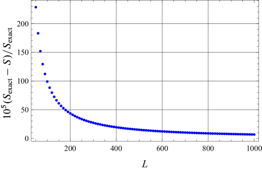
Figure 1: Relative error of the approximation (3.14) to the exact von Neumann entropy $S_{\mathrm{exact}}$ for $m=2$, $h_{1}=h_{2}=1/5$, $\alpha=1/2$ as a function of $L\in[50,1000]$ (in increments of $10$).

As expected, the maximum value of the entropies (3.13)-(3.14) is obtained when $n_{a}=1/(m+1)$ for all $a=1,\dots,m+1$, i.e., for $\mathbf{h}=0$. On the other hand, the approximations (3.13)–(3.14) to the von Neumann and Rényi entropies tend to $-\infty$ when $\mathbf{h}$ approaches the faces of the simplex ${\mathcal{H}}$, since each of these faces is determined by the vanishing of one of the magnon densities $n_{a}$. This behavior had already been pointed out in Ref. [17] for the von Neumann entropy of the isotropic ($\mathrm{su}(2)$) LMG model. It may seem surprising that the approximate von Neumann and Rényi entropies (3.13)–(3.14) become negative in a certain subset of ${\mathcal{H}}$. In fact, as we shall now discuss in more detail, when $L\gg 1$ the regions in which each of these approximations are negative (and, therefore, break down) are negligibly small.

In order to substantiate the previous claim, we shall estimate the distance $r_{0}$ of a point $\mathbf{h}_{0}$ lying on one of the $(m-1)$-dimensional faces of the simplex ${\mathcal{H}}$ to the positive entropy region, or equivalently to the zero entropy hypersurface. For simplicity, we shall deal with the generic situation in which $\mathbf{h}_{0}$ belongs to the interior of the face. We shall prove that for both entropies under consideration $r_{0}\sim L^{-m}$. To this end, suppose to begin with that $\mathbf{h}_{0}$ lies in the interior of the face where $n_{a}=0$, with $1\leqslant a\leqslant m$. In this case we can approximate the remaining densities $n_{b}$ by their values $n_{b}^{0}=h_{0b}+(1-h_{0})/(m+1)$ at the point $\mathbf{h}_{0}\equiv(h_{01},\dots,h_{0m})$ (with $h_{0}\equiv\sum_{a=1}^{m+1}h_{0a}$), so that (for instance) the von Neumann entropy satisfies

$$S\simeq\frac{m}{2}\,\log\big{[}2\pi\rme L(1-\alpha)\big{]}+\frac{1}{2}\hphantom{\hbox{$\scriptstyle 1\leqslant b$}}\sum_{\hbox to0.0pt{\hss$\scriptstyle 1\leqslant b\neq a\leqslant m+1$\hss}}\,\log n_{b}^{0}+\frac{1}{2}\,\log n_{a}\,.$$

Equating the RHS of this equation to zero and solving for $n_{a}$ we obtain

$$n_{a}\equiv\frac{1}{m+1}\,\left(mh_{a}-\sum_{\hbox to0.0pt{\hss$\scriptstyle 1\leqslant b\neq a\leqslant m+1$\hss}}h_{b}+1\right)=\frac{\big{[}2\pi\rme L(1-\alpha)]^{-m}}{\prod\limits_{\hbox to0.0pt{\hss$\scriptstyle 1\leqslant b\neq a\leqslant m+1$\hss}}n_{b}^{0}}\,.$$

Thus near $\mathbf{h}_{0}$ the $S=0$ hypersurface can be approximated by the above hyperplane, which is parallel to the hyperplane $n_{a}=0$ containing the face under consideration. Computing the distance between these two hyperplanes we immediately find the following approximate formula for $r_{0}$ in the case of the von Neumann entropy:

$$r_{0}\simeq\frac{m+1}{\sqrt{m^{2}+m-1}}\,\frac{\big{[}2\pi\rme L(1-\alpha)\big{]}^{-m}}{\prod\limits_{\hbox to0.0pt{\hss$\scriptstyle 1\leqslant b\neq a\leqslant m+1$\hss}}n_{b}^{0}}\sim L^{-m}\,.$$ (3.15)

When $\mathbf{h}_{0}$ lies on the face $n_{m+1}=0$ a totally analogous calculation leads to the slightly simpler result

$$r_{0}\simeq\frac{m+1}{\sqrt{m}}\,\frac{\big{[}2\pi\rme L(1-\alpha)\big{]}^{-m}}{\prod\limits_{\hbox to0.0pt{\hss$\scriptstyle 1\leqslant b\leqslant m$\hss}}n_{b}^{0}}\sim L^{-m}\,.$$ (3.16)

The computation of $r_{0}$ for the Rényi entropy proceeds along the same lines, with the result

$$r_{0}\simeq q^{\frac{m}{1-q}}\,\rme^{m}\,(r_{0})_{\mathrm{S}}\,,$$ (3.17)

where $(r_{0})_{\mathrm{S}}$ is the approximate value of $r_{0}$ for the von Neumann entropy given by Eqs. (3.15) or (3.16). Interestingly, the RHS of Eq. (3.17) is less (resp. greater) than $(r_{0})_{\mathrm{S}}$ for $0<q<1$ (resp. $q>1$). Note, finally, that the assumption that $\mathbf{h}_{0}$ belongs to the interior of the face is essential for the validity of Eqs. (3.15)–(3.17). More generally, it can be shown that the corresponding value of $r_{0}$ for $\mathbf{h}_{0}$ lying on (the interior of) an $(m-k)$-dimensional face of ${\mathcal{H}}$ (with $k=1,\dots,m$) behaves as $L^{-m/k}$. In other words, even in the most unfavorable case $k=m$ (i.e., when $\mathbf{h}_{0}$ is one of the vertices of the simplex ${\mathcal{H}}$) the distance of $\mathbf{h}_{0}$ to the positive entropy region is $\Or(L^{-1})$.

By Eqs. (3.13)-(3.14), when $L\to\infty$ the von Neumann and Rényi ground state entanglement entropies satisfy

$$S=R_{q} =\frac{m}{2}\log L+\Or(1)\,.$$ (3.18)

As remarked above, this behavior of the von Neumann entropy is characteristic of quantum critical (gapless) one-dimensional lattice systems with short-range interactions. More generally, when $d>1$ the von Neumann entanglement entropy of a $d$-dimensional critical system featuring short-range interactions is expected to scale as $L^{d-1}\log L$ (for fermionic systems) or $L^{d-1}$ (for bosonic ones) when $L\gg 1$, $L$ being the linear size of the system. On the other hand, for a non-critical (gapped) system with short-range interactions the von Neumann entropy should grow only as $L^{d-1}$. This so-called area law [9] has been verified for a wide range of quantum systems, such as the XX and XY models [6, 7], the Heisenberg (XYZ) spin chain [51, 52], the original ($\mathrm{su}(2)$, not necessarily isotropic) LMG model [17], translation-invariant (quadratic) fermionic systems in arbitrary dimension [53], and certain two-dimensional bosonic and fermionic systems [37], [54], to name only a few. On the other hand, for models with long-range interactions it is widely accepted that the area law need not hold, since in general the range of the interaction tends to increase the entropy [9]. This statement should be taken with some caution, since the entanglement entropy is ultimately a property of the state, and two models featuring short-range and long-range interactions may have the same ground state [55]. The logarithmic growth (3.18) of the ground state entanglement entropy of the gLMG models (2.13) does not indicate, however, that this class contains critical models. Indeed, the Rényi entropy of these models scales as $a\log L$ with $a$ independent of $q$, while for a two-dimensional CFT the coefficient $a$ should instead be proportional to $1+q^{-1}$.

It has been shown in Ref. [37] that in some low-dimensional quantum systems whose entanglement (von Neumann) entropy follows the area law the Tsallis entropy, defined by

$$T_{q}=\frac{\tr(\rho_{L}^{q})-1}{1-q}\,,$$ (3.19)

becomes extensive (i.e., scales as $L^{d}$, where $d$ is the number of space dimensions and $L$ is a characteristic length) for a suitable value of the positive parameter $q$. This entropy, which plays an important role in the study of strongly correlated classical systems, has also been extensively applied in other fields ranging from natural and social sciences to linguistics and economics (see the online document http://tsallis.cat.cbpf.br/TEMUCO.pdf for an updated bibliography). Since the Tsallis and Rényi entropies are obviously related by

$$R_{q}=\frac{\log\bigl{[}1+(1-q)T_{q}\bigr{]}}{1-q}\,,$$ (3.20)

from Eq. (3.13) we immediately obtain the following explicit formula for the Tsallis entanglement entropy of the ground state (2.7) of the gLMG model (2.13):

$$T_{q}=\frac{1}{1-q}\left(q^{-\frac{m}{2}}\left[2\pi L(1-\alpha)\prod_{a=1}^{m+1}n_{a}^{1/m}\right]^{\frac{m(1-q)}{2}}-1\right).$$ (3.21)

Thus for $L\gg 1$ the Tsallis entropy scales as a power law, namely

$$T_{q}=\frac{L^{\frac{m(1-q)}{2}}}{(1-q)q^{\frac{m}{2}}}\left[2\pi(1-\alpha)\prod_{a=1}^{m+1}n_{a}^{1/m}\right]^{\frac{m(1-q)}{2}}+\Or(1).$$ (3.22)

The dominant term of $T_{q}$ is linear in $L$ if $q=1-2/m$, which requires that $m\geqslant 3$ due to the condition $q>0$. For this critical value of $q$ the Tsallis entropy is given by

$$T_{1-\frac{2}{m}}=\frac{\pi mL(1-\alpha)}{{(1-\frac{2}{m})}^{\frac{m}{2}}}\prod_{a=1}^{m+1}n_{a}^{1/m}-\frac{m}{2}\,,$$ (3.23)

so that the entropy per particle in the thermodynamic limit reads

$$\lim_{L\to\infty}\frac{T_{1-\frac{2}{m}}}{L}=\frac{\pi m(1-\alpha)}{{(1-\frac{2}{m})}^{\frac{m}{2}}}\prod_{a=1}^{m+1}n_{a}^{1/m}\,.$$ (3.24)

As we have just seen, in the $\mathrm{su}(2)$ and $\mathrm{su}(3)$ cases the Tsallis entanglement entropy is not extensive for any value of the parameter $q$. It would therefore be of interest, in this context, to find a generalized entropy (like, e.g., one of the group entropies studied in Refs. [56] and [57]) which is extensive for the ground state of the gLMG model (2.13) with $m=1,2$.

4 Ground state phase diagram

In the previous sections we have studied the entanglement properties of the ground state of the gLMG model (2.13) when the magnetic field strength $\mathbf{h}$ lies in the interior of the simplex ${\mathcal{H}}$ given by Eq. (2.16). The aim of this section is to extend the previous results outside this region, determining how the behavior of the ground state and its entanglement entropy vary with $\mathbf{h}$.

To this end, note first of all that by Eq. (2.13) the magnon densities $n_{a}$ in the ground state must minimize the function

$$\varepsilon(n_{1},\dots,n_{m})=\sum_{a=1}^{m}c_{a}(n_{a}-n_{m+1}-h_{a})^{2}\,,$$ (4.1)

with $n_{m+1}=1-\sum\limits_{a=1}^{m}n_{a}$, in the simplex ${\mathcal{N}}\subset{\mathbb{R}}^{m}$ defined by

$$0\leqslant n_{a}\leqslant 1\,,\qquad\sum_{a=1}^{m}n_{a}\leqslant 1\,.$$

Thus the condition for the ground state to have well-defined magnon densities is that $\varepsilon$ has a unique minimum in ${\mathcal{N}}$. In fact, from the very definition of the set ${\mathcal{H}}$ it follows that for $\mathbf{h}\in{\mathcal{H}}$ the unique minimum of the energy function (4.1) over ${\mathbb{R}}^{m}$, given by Eqs. (2.14), lies in ${\mathcal{N}}$. More precisely, when $\mathbf{h}$ belongs to the interior of ${\mathcal{H}}$ the absolute minimum of $\varepsilon$ lies in the interior of ${\mathcal{N}}$, and therefore $0<n_{a}<1$ for all $a=1,\dots,m+1$. Thus in this case the ground state is not only entangled, but contains magnons of each of the $m+1$ types $|a\rangle$. On the other hand, when $\mathbf{h}$ belongs to the boundary of ${\mathcal{H}}$ the unique global minimum of $\varepsilon$, still given by Eq. (2.15), now lies on the boundary of ${\mathcal{N}}$. In particular, at least one of the magnon densities must vanish in this case, so that the ground state is entangled but does not have full magnon content. We shall be mainly interested in this section in the case in which $\mathbf{h}$ lies in the exterior of ${\mathcal{H}}$, so that the minimum of $\varepsilon$ in ${\mathcal{N}}$ is necessarily attained on its boundary $\partial{\mathcal{N}}$. This minimum is therefore no longer given by the simple equations (2.14), but must be computed by examining the behavior of $\varepsilon$ on $\partial{\mathcal{N}}$. We shall prove at the end of this section that the minimum of $\varepsilon$ on $\partial{\mathcal{N}}$ is unique for all values of the magnetic field strength $\mathbf{h}$. Thus the ground state of the generalized LMG model (2.13) is always unique, although its magnon content is given by Eq. (2.15) only for $\mathbf{h}\in{\mathcal{H}}$.

The boundary of the simplex ${\mathcal{N}}$ is the union of the $(m-k)$-dimensional sets (or $(m-k)$-faces) $\partial{\mathcal{N}}_{a_{1},\dots,a_{k}}$ determined by the equations

$$n_{a_{1}}=\cdots=n_{a_{k}}=0\,,$$

where $k=1,\dots,m$ and $1\leqslant a_{1}<\cdots<a_{k}\leqslant m+1$. Let us suppose, therefore, that the unique minimum of $\varepsilon$ in $\partial{\mathcal{N}}$ is attained on a certain $(m-k)$-face $\partial{\mathcal{N}}_{a_{1},\dots,a_{k}}$. If $k=m$ (i.e., if the minimum of $\varepsilon$ on ${\mathcal{N}}$ is attained at one of its vertices) then one of the magnon densities is necessarily equal to $1$ and the remaining ones vanish, so that the ground state is not entangled. On the other hand, if $1\leqslant k<m$ then the ground state is entangled but has not full magnon content, since it only contains magnons of $m-k+1<m+1$ types. In other words, we expect that in general the ground state can be in exactly one of $m+1$ possible “phases”, characterized by the vanishing of $0\leqslant k\leqslant m$ magnon densities. Note that we have included the $k=0$ case, in which $n_{a}>0$ for all $a=1,\dots,m+1$, which holds when $\mathbf{h}$ lies in the interior of ${\mathcal{H}}$.

We shall now describe the essential properties of the ground state when $\mathbf{h}$ belongs to the exterior of ${\mathcal{H}}$. As we have just seen, in this case the minimum of the energy function $\varepsilon$ is attained on one of the $(m-k)$-faces $\partial{\mathcal{N}}_{a_{1},\dots,a_{k}}$ of ${\mathcal{N}}$, so that in the ground state $n_{a_{1}}=\cdots=n_{a_{k}}=0$ and $0<n_{a_{k+1}},\dots,n_{a_{m+1}}<1$, where

$$\{a_{k+1},\dots,a_{m+1}\}=\{1,\dots,m+1\}\setminus\{a_{1},\dots,a_{k}\}\,.$$

Thus in the thermodynamic limit (3.3) we have

$$N_{a_{1}}=\cdots=N_{a_{k}}=L_{a_{1}}=\cdots=L_{a_{k}}=0\,,$$

and the eigenvalues of the reduced density matrix $\rho_{L}$ are given by

$$\lambda(L_{a_{k+1}},\dots,L_{a_{m}}) =\frac{L!}{\prod_{j=k+1}^{m+1}L_{a_{j}}!}\frac{(N-L)!}{\prod_{j=k+1}^{m+1}(N_{a_{j}}-L_{a_{j}})!}\frac{\prod_{j=k+1}^{m+1}N_{a_{j}}!}{N!}$$

$$={N\choose L}^{\!\!-1}\prod_{j=k+1}^{m+1}{N_{a_{j}}\choose L_{a_{j}}}\,,$$

with $L_{a_{m+1}}=L-\sum_{j=k+1}^{m}L_{a_{j}}$ . The distribution of the $m-k$ independent variables $L_{a_{j}}$ ($k+1\leqslant j\leqslant m$) is therefore the analogue of Eq. (3.2), with $m$ replaced by $m-k$ and $n_{1},\dots,n_{m+1}$ by $n_{a_{k+1}},\dots,n_{a_{m+1}}$. Hence Eqs. (3.13), (3.14) and (3.21) for the Rényi, von Neumann and Tsallis entropies still hold in this case, provided that we perform the above replacements; in particular, the von Neumann entropy is given by

$$S=\frac{m-k}{2}\log\left(2\pi\rme L(1-\alpha)\prod_{j=k+1}^{m+1}n_{a_{j}}^{1/(m-k)}\right)\,.$$ (4.2)

In the derivation of the latter equation we have tacitly assumed that $k<m$. In fact, when $k=m$ the ground state is not entangled, and hence $S=0$ in this case.

By Eq. (4.2), the asymptotic behavior of the von Neumann entropy in the ground state phase with $k$ vanishing magnon densities is given by

$$S=\frac{m-k}{2}\,\log L+\Or(1)\,.$$

As discussed in the previous section, this result does not imply that in this phase there should be critical gLMG models. Indeed, the Rényi entropy $R_{q}$ also scales as $a\log L$ when $L\gg 1$, where $a=(m-k)/2$ is independent of the parameter $q$. As we know, this behavior is inconsistent with the characteristic scaling of the Rényi entropy of a one-dimensional CFT, for which $R_{q}=a(q)\log L$ with $a(q)$ proportional to $1+q^{-1}$.

Remark 6.

By the discussion preceding Eq. (4.2), the Tsallis entropy in the phase with $k$ vanishing magnon densities scales as $L^{(m-k)(1-q)/2}$, and is therefore extensive for $q=1-2/(m-k)$ provided that $m-k\geqslant 3$. Hence this entropy is not extensive for any value of $q$ in the phases with $m-1$ and $m-2$ vanishing magnon densities.

As a concrete example of the previous general statements, we shall next discuss in detail the $\mathrm{su}(3)$ case ($m=2$) with the symmetric choice $c_{1}=c_{2}=C$. Taking (without loss of generality) $C=1$, the energy function is simply

$$\varepsilon(\mathbf{n})=\big{(}\mathbf{x}(\mathbf{n})-\mathbf{h}\big{)}^{2}\,,$$ (4.3)

where $\mathbf{x}(\mathbf{n})\equiv\sum_{s=1}^{3}n_{s}\boldsymbol{\mu}_{s}$, $\mathbf{n}=(n_{1},n_{2})\in{\mathcal{N}}$ and $n_{3}=1-n_{1}-n_{2}$. When $\mathbf{n}$ ranges over ${\mathcal{N}}$, the point $\mathbf{x}(\mathbf{n})$ varies over the triangle ${\mathcal{H}}$ in a one-to-one fashion, with $\mathbf{n}\in\partial{\mathcal{N}}$ if and only if $\mathbf{x}(\mathbf{n})\in\partial{\mathcal{H}}$. Hence the minimum of $\varepsilon(\mathbf{n})$ is simply the distance of the fixed vector $\mathbf{h}$ to the triangle ${\mathcal{H}}$. Moreover, since this triangle is convex, the minimum distance of $\mathbf{h}$ to ${\mathcal{H}}$ is attained at a unique point $\mathbf{x}(\mathbf{n}_{0})$ in ${\mathcal{H}}$.

The problem of minimizing the energy function $\varepsilon$ has a very simple geometric solution. Indeed, when $\mathbf{h}\in\,\mathop{\!{\mathcal{H}}}\limits^{\lower 3.01389pt\hbox{$\scriptstyle\circ$}}{}$ the point $\mathbf{x}(\mathbf{n}_{0})$ closest to $\mathbf{h}$ is obviously $\mathbf{h}$ itself, so that the magnon density vector $\mathbf{n}_{0}=\mathbf{x}^{-1}(\mathbf{h})$ is given by Eq. (2.15). Suppose, on the other hand, that $\mathbf{h}\notin\,\mathop{\!{\mathcal{H}}}\limits^{\lower 3.01389pt\hbox{$\scriptstyle\circ$}}{}$ (including the limiting case $\mathbf{h}\in\partial{\mathcal{H}}$). Let us denote by $L_{bc}$ the side of the triangle ${\mathcal{H}}$ with vertices $\boldsymbol{\mu}_{b}$ and $\boldsymbol{\mu}_{c}$. This side is parametrized by a magnon density $\mathbf{n}$ with $n_{a}=0$, where $\{a,b,c\}=\{1,2,3\}$. Likewise, we shall denote by $R_{bc}$ the half-strip bounded by the side $L_{bc}$ and the two straight lines perpendicular to it through the vertices $\boldsymbol{\mu}_{b}$ and $\boldsymbol{\mu}_{c}$ which does not contain the opposite vertex $\boldsymbol{\mu}_{a}$, with the two limiting half-lines removed (cf. Fig. 2). By construction, when $\mathbf{h}\in R_{bc}$ the point in ${\mathcal{H}}$ closest to $\mathbf{h}$ lies on the interior of the side $L_{bc}\subset\partial{\mathcal{H}}$, so that in this case the corresponding density $\mathbf{n}_{0}$ belongs to the side $n_{a}=0$ of ${\mathcal{N}}$. The value of $\mathbf{n}_{0}\equiv(n_{01},n_{02})$ can be easily computed by minimizing

$$\varepsilon\big{|}_{n_{a}=0}=\Big{(}n_{b}(\boldsymbol{\mu}_{b}-\boldsymbol{\mu}_{c})+\boldsymbol{\mu}_{c}-\mathbf{h}\Big{)}^{\!2}$$ (4.4)

with respect to $n_{b}$ (assuming, without loss of generality, that $b\in\{1,2\}$). In this way we easily obtain

$$n_{0b}=\frac{(\mathbf{h}-\boldsymbol{\mu}_{c})\cdot(\boldsymbol{\mu}_{b}-\boldsymbol{\mu}_{c})}{(\boldsymbol{\mu}_{b}-\boldsymbol{\mu}_{c})^{2}}\,,$$ (4.5)

and of course $n_{0c}=1-n_{0b}$. Note that in this case, although $n_{0a}=0$, the ground state is still entangled, since $0<n_{0b},n_{0c}<1$. On the other hand, let $W_{a}$ denote the closed wedge with vertex $\boldsymbol{\mu}_{a}$ limited by the half-strips $R_{ab}$ and $R_{ac}$ (cf. Fig. 2). Obviously, if $\mathbf{h}$ lies in $W_{a}$ the point of the triangle ${\mathcal{H}}$ closest to $\mathbf{h}$ is the vertex $\boldsymbol{\mu}_{a}$, whose corresponding magnon densities are $n_{a}=1$ and $n_{b}=n_{c}=0$.

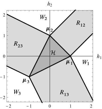
Figure 2: Triangle ${\mathcal{H}}$, half-strips $R_{ab}$, wedges $W_{a}$ and vertices $\boldsymbol{\mu}_{a}$ in the $(h_{1},h_{2})$-plane.

In summary, we have shown that the “phase diagram” of the ground state of the $\mathrm{su}(3)$ gLMG model (2.13) (with $c_{1}=c_{2}$ for all $a$) is as follows:

1. In the interior $\,\mathop{\!{\mathcal{H}}}\limits^{\lower 3.01389pt\hbox{$\scriptstyle\circ$}}{}$ of the triangle ${\mathcal{H}}$, the ground state is a symmetric state containing all three types of magnons $|a\rangle$ (with $a=1,2,3$).

2. In each of the sets $R_{bc}$ the ground state is still entangled, but contains only magnons of the two types $|b\rangle$ and $|c\rangle$.

3. In the wedges $W_{a}$, the ground state consists of magnons of type $|a\rangle$ only, and is therefore not entangled.

From the previous remark, the general formula (4.2) and Eqs. (2.15) and (4.5), it follows that when $L\gg 1$ the von Neumann entanglement entropy as a function of the $\mathrm{su}(3)$ magnetic field strength $\mathbf{h}$ is given by

$$S=\cases{S_{0}-\frac{3}{2}\log 3+\frac{1}{2}\,\Big{(}\log(1+2h_{1}-h_{2})+\log(1-h_{1}+2h_{2})&\vspace*{-.5\baselineskip}\\ \hphantom{S_{0}-\frac{3}{2}\log 3+\frac{1}{2}\,\big{(}\log(2h_{1}-h_{2}-1)+\log(2h_{2}-}+\log(1-h_{1}-h_{2})\Big{)},&$\mathbf{h}\in\,\mathop{\!{\mathcal{H}}}\limits^{\lower 3.01389pt\hbox{$\scriptstyle\circ$}}{}$\\ \frac{1}{2}\Big{(}S_{0}+\log\left[1-(h_{1}-h_{2})^{2}\right]-2\log 2\Big{)},&\hphantom{$\mathbf{h}\in\,\mathop{\!{\mathcal{H}}}\limits^{\lower 3.01389pt\hbox{$\scriptstyle\circ$}}{}$}\hbox to0.0pt{\hss$\mathbf{h}\in R_{12}$}\\ \frac{1}{2}\Big{(}S_{0}-2\log 5+\log(3+2h_{1}+h_{2})+\log(2-2h_{1}-h_{2})\Big{)},&\hphantom{$\mathbf{h}\in\,\mathop{\!{\mathcal{H}}}\limits^{\lower 3.01389pt\hbox{$\scriptstyle\circ$}}{}$}\hbox to0.0pt{\hss$\mathbf{h}\in R_{13}$}\\ \frac{1}{2}\Big{(}S_{0}-2\log 5+\log(3+h_{1}+2h_{2})+\log(2-h_{1}-2h_{2})\Big{)},&\hphantom{$\mathbf{h}\in\,\mathop{\!{\mathcal{H}}}\limits^{\lower 3.01389pt\hbox{$\scriptstyle\circ$}}{}$}\hbox to0.0pt{\hss$\mathbf{h}\in R_{23}$}\\ 0\,,&\hphantom{$\mathbf{h}\in\,\mathop{\!{\mathcal{H}}}\limits^{\lower 3.01389pt\hbox{$\scriptstyle\circ$}}{}$}\hbox to0.0pt{\hss$\mathbf{h}\in W_{1}\cup W_{2}\cup W_{3}\,,$}}$$

with $S_{0}\equiv\log\bigl{[}2\pi\rme L(1-\alpha)\bigr{]}$ . In Fig. 3 we have plotted this entropy as a function of the magnetic field $\mathbf{h}$ in the range $|h_{a}|\leqslant 2$ for $L(1-\alpha)=1000$. As mentioned in the previous section, the latter approximation to the von Neumann entropy tends to $-\infty$ when $\mathbf{h}$ approaches a side $L_{ab}$ of the triangle ${\mathcal{H}}$ from its interior. Note, however, that it has a finite limit when this side is approached from the corresponding half-strip $R_{ab}$. Similarly, $S\to-\infty$ when $\mathbf{h}$ approaches one of the straight lines limiting a half-strip $R_{ab}$ from its interior, but has a finite limit when this straight line is approached from the corresponding wedge $W_{a}$ or $W_{b}$ (except at the vertices $\boldsymbol{\mu}_{a}$ and $\boldsymbol{\mu}_{b}$).

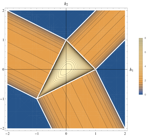
Figure 3: Von Neumann entropy of the $\mathrm{su}(3)$ gLMG model (2.13) with $c_{1}=c_{2}$ and $L(1-\alpha)=1000$ as a function of the magnetic field $\mathbf{h}=(h_{1},h_{2})$.

Remark 7.

A formula similar to the previous equation for the von Neumann entropy can be derived without difficulty for the Rényi and the Tsallis entropies. In fact, comparing Eqs. (3.13)-(3.14) it is clear that the only difference between the von Neumann and the Rényi entropies is the constant term $(m-k)[(\log q)/(q-1)-1]/2$ in the phase with $k$ vanishing magnon densities (i.e., $k=0,1,2$ respectively for $\mathbf{h}$ belonging to $\,\mathop{\!{\mathcal{H}}}\limits^{\lower 3.01389pt\hbox{$\scriptstyle\circ$}}{}$, $R_{ab}$ and $W_{a}$). Thus the von Neumann and Rényi entropies are essentially equivalent for the models under consideration.

In the general case (i.e., for $m>2$ and arbitrary positive values of the parameters $c_{a}$), the analysis is very similar. Indeed, in this case the energy function $\varepsilon(\mathbf{n})$ can be written as

$$\varepsilon(\mathbf{n})=\|\mathbf{x}(\mathbf{n})-\mathbf{h}\|^{2}\,,$$

where

$$\mathbf{x}(\mathbf{n})=\sum_{s=1}^{m+1}n_{s}\boldsymbol{\mu}_{s}\,,\qquad\mathbf{n}=(n_{1},\dots,n_{m})\,,\qquad n_{m+1}=1-\sum_{a=1}^{m}n_{a}\,,$$

and the norm $\|{\cdot}\|$ is defined by $\|\mathbf{y}\|^{2}\equiv\sum_{a=1}^{m}c_{a}y_{a}^{2}$. As before, when the vector $\mathbf{n}$ varies over the simplex ${\mathcal{N}}$ the point $\mathbf{x}(\mathbf{n})$ parametrizes the simplex ${\mathcal{H}}$ in a bijective way, with $\mathbf{n}\in\partial{\mathcal{N}}$ if and only if $\mathbf{x}(\mathbf{n})\in\partial{\mathcal{H}}$. Thus the problem of minimizing $\varepsilon(\mathbf{n})$ is again equivalent to finding the distance (with respect to the norm $\|{\cdot}\|$) of the fixed vector $\mathbf{h}$ to the simplex ${\mathcal{H}}$. Since this simplex is a convex polytope, there is a unique point in ${\mathcal{H}}$ closest to $\mathbf{h}$ for all values of $\mathbf{h}\in{\mathbb{R}}^{m}$. This proves that the magnon densities are uniquely determined by the magnetic field strength $\mathbf{h}$, so that the ground state of the gLMG model (2.13) is always unique. More precisely, when $\mathbf{h}\in\,\mathop{\!{\mathcal{H}}}\limits^{\lower 3.01389pt\hbox{$\scriptstyle\circ$}}{}$, the distance of $\mathbf{h}$ to ${\mathcal{H}}$ is obviously zero and the corresponding density vector $\mathbf{n}_{0}$ is again determined by the condition $\mathbf{h}=\mathbf{x}(\mathbf{n}_{0})$, i.e., by Eq. (2.15). On the other hand, when $\mathbf{h}$ lies outside $\,\mathop{\!{\mathcal{H}}}\limits^{\lower 3.01389pt\hbox{$\scriptstyle\circ$}}{}$ (in particular, if $\mathbf{h}\in\partial{\mathcal{H}}$), it is clear from geometric considerations that the minimum distance of $\mathbf{h}$ to the simplex ${\mathcal{H}}$ is attained at a point $\mathbf{x}(\mathbf{n}_{0})\in\partial{\mathcal{H}}$, so that the corresponding magnon density $\mathbf{n}_{0}$ lies in $\partial{\mathcal{N}}$. Hence in the latter case the system is in one of the $m$ phases characterized by the vanishing of $k>0$ magnon densities.

5 Conclusions and outlook

In this work we have introduced a large class of $\mathrm{su}(m+1)$ spin models with long-range interactions possessing a symmetric non-degenerate ground state with well-defined magnon numbers. Our models provide a natural multiparameter generalization of the well-known spin $1/2$ isotropic Lipkin–Meshkov–Glick model, featuring non-constant interactions and $\mathrm{su}(m+1)$ spin. They are also closely related to Haldane–Shastry type chains, which can be formally obtained from them through specific realizations of the couplings $h_{ij}$ dropping the magnetic field terms.

One of the main results of our work is the detailed derivation of the asymptotic behavior of the eigenvalues of the reduced density matrix of a block of $L$ spins when the system is in its ground state, for arbitrary values of $m$ and $\alpha=\lim_{N\to\infty}L/N$. This makes it possible to compute the von Neumann and Rényi entropies in closed form when $L\gg 1$, and to derive their asymptotic behavior when $L\to\infty$. A notable outcome of our analysis is that both of these entropies scale as $\frac{1}{2}(m-k)\log L$ in the latter limit, where $k$ is the number of vanishing magnon densities in the ground state. In particular, from the behavior of the Rényi entropy it follows that the class of generalized $\mathrm{su}(m+1)$ LMG models contains no critical models. We have also computed the Tsallis entropy, showing that it can be made extensive when the number of “effective” internal degrees of freedom $m-k+1$ is greater than $3$. Finally, we have completely determined the different phases of the ground state in terms of the $\mathrm{su}(m+1)$ magnetic field strength $\mathbf{h}$, and shown that they are related in a simple geometric way to the weights of the fundamental representation of $\mathrm{su}(m+1)$.

Our results open up several natural directions for further research and a number of related problems. One such problem is the determination in closed form of the full spectrum of suitable models of the class introduced in this paper, particularly for $\mathrm{su}(m+1)$ spin with $m>1$. In fact, the integrability properties of the HS-type chains suggest the possibility of exploring the existence of integrable generalizations thereof with a non-vanishing magnetic field term of the form considered in this work. At the same time, it could also be of interest to extend the analysis of the entanglement entropy performed in this paper to different entropic functionals. Indeed, due to the presence of several parameters in the gLMG Hamiltonian, multiparametric entropies [56, 57] could play an important role in the classification of the possible thermodynamic regimes admitted by the system when one varies the values of its parameters. Finally, the fact that the von Neumann entanglement entropy of generalized LMG models is proportional to $\log L$ in certain regions of parameter space, though as we have seen does not imply the existence of critical models, suggests that these regions may nevertheless contain models with interesting non-generic properties worth investigating. This is certainly true in the $m=1$ case, since (for instance) the isotropic LMG model is gapless precisely in the interval $|h|<1$ for which the von Neumann entropy scales as $\log L$ [40].

Appendix A Ground-state reduced density matrix for a block of spins

In this appendix we shall compute from first principles the reduced density matrix $\rho_{L}$ of a block of $L$ spins of the $\mathrm{su}(m+1)$ gLMG chain (2.13) when the system is in its ground state (2.7), with magnon densities $n_{a}=N_{a}/N$ determined (in the thermodynamic limit) by Eq. (2.15). This result, first obtained in Ref. [30], shall be used in Section 3 to evaluate several standard bipartite entanglement entropies in the thermodynamic limit.

More precisely, we need to compute

$$\rho_{L}=\tr_{N-L}\rho\equiv\tr_{N-L}|\psi(N_{1},\dots,N_{m+1})\rangle\langle\psi(N_{1},\dots,N_{m+1})|\,,$$ (1.1)

where $\tr_{N-L}$ is the trace over the degrees of freedom of the remaining $N-L$ spins. Since the ground state $|\psi(N_{1},\dots,N_{m+1})\rangle$ is invariant under permutations, the result is obviously independent of the specific positions of the $L$ spins considered. We shall therefore assume in what follows that the two blocks under consideration consist of the first $L$ and the last $N-L$ spins. In order to evaluate the RHS of Eq. (1.1), it is convenient to label the states of the canonical spin basis $|s_{1},\dots,s_{N}\rangle$ by the positions of its magnons. More explicitly, we shall use the notation $|\mathbf{i}_{1},\dots,\mathbf{i}_{m}\rangle$ to denote a state whose type $a$ magnons (with $a=1,\dots,m$) are located in the positions specified by the $N_{a}$ components of the ordered multi-index $\mathbf{i}_{a}$, while those of type $m+1$ lie in the remaining positions. Note, in particular, that no two multi-indices $\mathbf{i}_{a}$ and $\mathbf{i}_{b}$ with $a\neq b$ can have any common components, which we shall denote by $\mathbf{i}_{a}\cap\mathbf{i}_{b}=\emptyset$. For instance, with this notation the $\mathrm{su}(4)$ basis state $|3,1,1,4,1,3,4\rangle$ will be denoted by $|(2,3,5),(),(1,6)\rangle$.

Using the above notation, the ground state (2.7) can be written as

$$|\psi(N_{1},\dots,N_{m+1})\rangle=\left(\frac{N!}{\prod_{a=1}^{m+1}N_{a}!}\right)^{\!\!-\frac{1}{2}}\sum_{\mathbf{i}_{1},\dots,\mathbf{i}_{m}}|\mathbf{i}_{1},\dots,\mathbf{i}_{m}\rangle\,,$$ (1.2)

where the sum is over all ordered multi-indices $\mathbf{i}_{a}\in\{1,\dots,N\}^{N_{a}}$ such that $\mathbf{i}_{a}\cap\mathbf{i}_{b}=\emptyset$ for $a\neq b$. We thus have

$$\rho=\frac{\prod_{a=1}^{m+1}N_{a}!}{N!}\sum_{\substack{\mathbf{i}_{1},\dots,\mathbf{i}_{m}\cr\mathbf{j}_{1},\dots,\,\mathbf{j}_{m}}}|\mathbf{i}_{1},\dots,\mathbf{i}_{m}\rangle\langle\,\mathbf{j}_{1},\dots,\mathbf{j}_{m}|\,,$$

where the sum is again over all ordered multi-indices $\mathbf{i}_{a}$, $\mathbf{j}_{a}$ satisfying the above condition. Thus, in order to evaluate $\rho_{L}$ we need only compute $\tr_{N-L}|\mathbf{i}_{1},\dots,\mathbf{i}_{m}\rangle\langle\,\mathbf{j}_{1},\dots,\mathbf{j}_{m}|$. To this end, we decompose each multi-index $\mathbf{i}_{a}$ as

$$\mathbf{i}_{a}=(\mathbf{i}_{a}^{L},\mathbf{i}_{a}^{N-L})\,,$$

where the components of each  $\mathbf{i}_{a}^{L}$ range from $1$ to $L$ and those of $\mathbf{i}_{a}^{N-L}$ from $L+1$ to $N$, and similarly for $\mathbf{j}_{a}$. It is then straightforward to show that

$$\tr_{N-L}|\mathbf{i}_{1},\dots,\mathbf{i}_{m}\rangle\langle\,\mathbf{j}_{1},\dots,\mathbf{j}_{m}|=|\mathbf{i}_{1}^{L},\dots,\mathbf{i}_{m}^{L}\rangle\langle\,\mathbf{j}_{1}^{L},\dots,\mathbf{j}_{m}^{L}|\,\prod_{a=1}^{m}\delta_{\mathbf{i}_{a}^{N-L},\,\mathbf{j}_{a}^{N-L}}\,.$$ (1.3)

Indeed,

$$\langle s_{L+1},\dots,s_{N}|\mathbf{i}_{1},\dots,\mathbf{i}_{m}\rangle\,\langle\,\mathbf{j}_{1},\dots,\mathbf{j}_{m}|s_{L+1},\dots,s_{N}\rangle=0$$

unless the last $N-L$ spin components of the basis states represented by $|\mathbf{i}_{1},\dots,\mathbf{i}_{m}\rangle$ and $|\,\mathbf{j}_{1},\dots,\mathbf{j}_{m}\rangle$ are both equal to $s_{L+1},\dots,s_{N}$, which accounts for the product of Kronecker deltas in Eq. (1.3). Moreover, when $\mathbf{i}_{a}^{N-L}=\mathbf{j}_{a}^{N-L}$ for all $a=1,\dots,m$ the only state of the canonical basis of the Hilbert space of the last $N-L$ spins that can contribute to the trace is $|\mathbf{i}_{1}^{N-L},\dots,\mathbf{i}_{m}^{N-L}\rangle=|\mathbf{j}_{1}^{N-L},\dots,\mathbf{j}_{m}^{N-L}\rangle$, which immediately yields Eq. (1.3).

Using Eq. (1.3) it is straightforward to obtain the expression

$$\rho_{L}=\frac{\prod_{a=1}^{m+1}N_{a}!}{N!}\sum_{\substack{\mathbf{i}_{1}^{L},\dots,\mathbf{i}_{m}^{L},\,\mathbf{j}_{1}^{L},\dots,\,\mathbf{j}_{m}^{L}\,,\mathbf{i}_{1}^{N-L},\dots,\mathbf{i}_{m}^{N-L}\cr|\mathbf{i}_{a}^{L}|=|\mathbf{j}_{a}^{L}|=N_{a}-|\mathbf{i}_{a}^{N-L}|}}|\mathbf{i}_{1}^{L},\dots,\mathbf{i}_{m}^{L}\rangle\langle\,\mathbf{j}_{1}^{L},\dots,\mathbf{j}_{m}^{L}|\,,$$ (1.4)

where $|\mathbf{i}|$ denotes the number of components of the multi-index $\mathbf{i}$. In order to evaluate the latter sum, we introduce the notation $L_{a}=|\mathbf{i}_{a}^{L}|$, $a=1,\dots,m$, where the magnon numbers $L_{1},\dots,L_{m}$ satisfy the obvious inequalities

$$0\leqslant L_{a}\leqslant N_{a}\,,\qquad\sum_{a=1}^{m}L_{a}\leqslant L\,,\qquad\sum_{a=1}^{m}(N_{a}-L_{a})\leqslant N-L\,.$$ (1.5)

Equation (1.4) can then be written as

$$\rho_{L}=\frac{\prod_{a=1}^{m+1}N_{a}!}{N!}\sum_{L_{1},\dots,L_{m}}\,\sum_{\substack{\mathbf{i}_{1}^{L},\dots,\mathbf{i}_{m}^{L},\,\mathbf{j}_{1}^{L},\dots,\,\mathbf{j}_{m}^{L}\cr|\mathbf{i}_{a}^{L}|=|\mathbf{j}_{a}^{L}|=L_{a}}}\sum_{\substack{\mathbf{i}_{1}^{N-L},\dots,\mathbf{i}_{m}^{N-L}\cr|\mathbf{i}_{a}^{N-L}|=N_{a}-L_{a}}}|\mathbf{i}_{1}^{L},\dots,\mathbf{i}_{m}^{L}\rangle\langle\,\mathbf{j}_{1}^{L},\dots,\mathbf{j}_{m}^{L}|\,,$$ (1.6)

where the outermost sum is over the range specified by Eq. (1.5). The sum over the multi-indices $\mathbf{i}_{a}^{N-L}$ is clearly the number of different $(N-L)$-particles states of the form $|\mathbf{i}_{1}^{N-L},\dots,\mathbf{i}_{m}^{N-L}\rangle$ with a fixed number $N_{a}-L_{a}$ of type $a$ magnons ($1\leqslant a\leqslant m+1$), namely the combinatorial number

$$\frac{(N-L)!}{\prod_{a=1}^{m+1}(N_{a}-L_{a})!}$$

with $L_{m+1}\equiv L-\sum\limits_{a=1}^{m}L_{a}$. Thus Eq. (1.6) reduces to

$$\rho_{L}=\frac{\prod_{a=1}^{m+1}N_{a}!}{N!}\sum_{L_{1},\dots,L_{m}}\frac{(N-L)!}{\prod_{a=1}^{m+1}(N_{a}-L_{a})!}\sum_{\substack{\mathbf{i}_{1}^{L},\dots,\mathbf{i}_{m}^{L}\cr|\mathbf{i}_{a}^{L}|=L_{a}}}|\mathbf{i}_{1}^{L},\dots,\mathbf{i}_{m}^{L}\rangle\cdot\sum_{\substack{\mathbf{j}_{1}^{L},\dots,\,\mathbf{j}_{m}^{L}\cr|\mathbf{j}_{a}^{L}|=L_{a}}}\langle\,\mathbf{j}_{1}^{L},\dots,\mathbf{j}_{m}^{L}|\,.$$

Using Eq. (1.2) with $N$ and $N_{a}$ respectively replaced by $L$ and $L_{a}$ we finally arrive at the following explicit formula for the reduced density matrix $\rho_{L}$:

$$\rho_{L}=\sum_{L_{1},\dots,L_{m}}\lambda(L_{1},\dots,L_{m})|\psi(L_{1},\dots,L_{m+1})\rangle\langle\psi(L_{1},\dots,L_{m+1})|\,,$$ (1.7)

where the summation range is again given by Eq. (1.5) and

$$\lambda(L_{1},\dots,L_{m})=\frac{L!}{\prod_{a=1}^{m+1}L_{a}!}\,\frac{(N-L)!}{\prod_{a=1}^{m+1}(N_{a}-L_{a})!}\,\frac{\prod_{a=1}^{m+1}N_{a}!}{N!}={N\choose L}^{\!\!-1}\prod_{a=1}^{m+1}{N_{a}\choose L_{a}}\,.$$ (1.8)

Thus $\rho_{L}$ is diagonal in the basis $|\psi(L_{1},\dots,L_{m+1})\rangle$ with $L_{1},\dots,L_{m}$ satisfying (1.5) (and $L_{m+1}=L-\sum_{a=1}^{m}L_{a}$), and its eigenvalues $\lambda(L_{1},\dots,L_{m})$ are given by Eq. (1.8) (cf. [30]). In the particular case $m=1$ (1.8) reduces to a hypergeometric distribution [58], as shown in Ref. [17] for the isotropic LMG model (see also [16]).

According to the Schmidt decomposition theorem (see, e.g., [2]), the ground state $|\psi(N_{1},\dots,N_{m+1})\rangle$ can be expressed as

$$|\psi(N_{1},\dots,N_{m+1})\rangle=\sum_{i}b_{i}|\psi_{i}\rangle\otimes|\varphi_{i}\rangle\,,$$ (1.9)

where $\{|\psi_{j}\rangle\}$ and $\{|\varphi_{k}\rangle\}$ are appropriate orthonormal bases of the Hilbert spaces of the first $L$ and last $N-L$ particles, and the Schmidt coefficients $b_{i}$ are non-negative real numbers. From this formula it immediately follows that

$$\rho_{L}=\sum_{i}b_{i}^{2}\,|\psi_{i}\rangle\langle\psi_{i}|\,,$$

and comparing with Eq. (1.7) we obtain

$$|\psi_{i}\rangle=|\psi(L_{1},\dots,L_{m+1})\rangle\,,\qquad b_{i}=\sqrt{\lambda(L_{1},\dots,L_{m+1})}\,.$$

In fact, in this case it is straightforward to derive the Schmidt decomposition (1.9) directly. Indeed, using the previous notation for the multi-indices $\mathbf{i}_{a}$ and Eq. (1.2) we have

Again, in the $\mathrm{su}(2)$ case the latter equation reduces to the analogous formula in Ref. [17].

It is also important to observe that all the results in this section are based exclusively on the fact that the ground state of the gLMG model (2.13) is of the form (2.7), i.e., it is symmetric and has well-defined magnon densities. Thus the above results hold, in general, for any quantum system whose ground state is of the latter form.

Appendix B Moments of the multivariate hypergeometric distribution

In this appendix we shall compute in closed form the first and second moments of the multivariate hypergeometric distribution $\lambda(L_{1},\dots,L_{m})$ given by Eq. (3.2), with support (1.5). Our starting point is the elementary identity

$$\prod_{i=1}^{m+1}(1+t_{i})^{N_{i}}=\sum_{L_{1}=0}^{N_{1}}\cdots\sum_{L_{m+1}=0}^{N_{m+1}}\prod_{i=1}^{m+1}{N_{i}\choose L_{i}}\cdot t_{1}^{L_{1}}\cdots t_{m+1}^{L_{m+1}}\,,$$

from which we deduce that

$$\sum_{L_{1}=0}^{N_{1}}\cdots\sum_{L_{m+1}=0}^{N_{m+1}}\prod_{k=1}^{n}(L_{i}-k+1)\cdot\prod_{j=1}^{m+1}{N_{j}\choose L_{j}}\cdot t_{1}^{L_{1}}\cdots t_{m+1}^{L_{m+1}}=t_{i}^{n}\frac{\partial^{n}}{\partial t_{i}^{n}}\,\prod_{j=1}^{m+1}(1+t_{j})^{N_{j}}.$$ (2.1)

The previous formula can be applied to compute the moments of the distribution $\lambda(L_{1},\dots,L_{m})$ in a straightforward way. Indeed, let

$$\langle f(L_{1},\dots,L_{m})\rangle\equiv\sum_{L_{1},\dots,L_{m}}f(L_{1},\dots,L_{m})\lambda(L_{1},\dots,L_{m})\,,$$

where the sum ranges over the set determined by the inequalities (1.5), denote the average of the function $f(L_{1},\dots,L_{m})$ with respect to the distribution (3.2). Equation (2.1) with $N_{1}+\cdots+N_{m+1}=N$ implies that

$$\left\langle\prod_{k=1}^{n}(L_{i}-k+1)\right\rangle={N\choose L}^{-1}\left\{t_{i}^{n}\frac{\partial^{n}}{\partial t_{i}^{n}}\,\prod_{j=1}^{m+1}(1+t_{j})^{N_{j}}\Big{|}_{t_{1}=\cdots=t_{m+1}=t}\right\}_{L},$$ (2.2)

where $\{\phi(t)\}_{L}$ denotes the coefficient of $t^{L}$ in the polynomial $\phi(t)$. From the latter formula with $n=1$ we obtain

$$\langle L_{i}\rangle={N\choose L}^{-1}\left\{N_{i}t(1+t)^{N-1}\right\}_{L}=N_{i}\,\frac{{N-1\choose L-1}}{{N\choose L}}=\frac{LN_{i}}{N}=Ln_{i}\,.$$ (2.3)

Similarly, Eq. (2.2) with $n=2$ yields

$$\big{\langle}L_{i}(L_{i}-1)\big{\rangle} ={N\choose L}^{-1}\left\{N_{i}(N_{i}-1)t^{2}(1+t)^{N-2}\right\}_{L}=N_{i}(N_{i}-1)\,\frac{{N-2\choose L-2}}{{N\choose L}}$$

$$=\frac{L(L-1)N_{i}(N_{i}-1)}{N(N-1)}\,,$$

so that

$$\big{\langle}x_{i}^{2}\big{\rangle}\equiv\Big{\langle}(L_{i}-\langle L_{i}\rangle)^{2}\Big{\rangle}=\big{\langle}L_{i}(L_{i}-1)\big{\rangle}-\langle L_{i}\rangle\big{(}\langle L_{i}\rangle-1\big{)}=Ln_{i}(1-n_{i})\,\frac{N-L}{N-1}\,.$$ (2.4)

In particular, in the thermodynamic limit $N\to\infty$ with $\lim_{N\to\infty}(L/N)=\alpha$ finite we obtain the asymptotic formula

$$\big{\langle}x_{i}^{2}\big{\rangle}\simeq L(1-\alpha)n_{i}(1-n_{i})\,.$$ (2.5)

The latter equation generalizes the analogous formula derived in Ref. [30] by approximating $\lambda(L_{1},\dots,L_{m})$ by a multinomial distribution, valid only for $\alpha=0$. Finally, the covariances $\langle x_{i}x_{j}\rangle=\langle L_{i}L_{j}\rangle-\langle L_{i}\rangle\langle L_{j}\rangle$ with $i\neq j$ can also be easily evaluated from the identity

$$\left\langle L_{i}L_{j}\right\rangle={N\choose L}^{-1}\left\{t_{i}t_{j}\frac{\partial}{\partial t_{i}}\frac{\partial}{\partial t_{j}}\,\prod_{k=1}^{m+1}(1+t_{k})^{N_{k}}\Big{|}_{t_{1}=\cdots=t_{m+1}=t}\right\}_{L},$$ (2.6)

whose proof is similar to that of Eq. (2.2). From Eq. (2.6) we easily obtain

$$\left\langle L_{i}L_{j}\right\rangle={N\choose L}^{-1}\left\{N_{i}N_{j}t^{2}(1+t)^{N-2}\right\}_{L}=N_{i}N_{j}$$

=L(L-1)NiNjN(N-1),i≠j,

and hence, by Eq. (2.3),

$$\big{\langle}x_{i}x_{j}\big{\rangle}=\frac{L(L-1)N_{i}N_{j}}{N(N-1)}-\frac{L^{2}N_{i}N_{j}}{N^{2}}=-Ln_{i}n_{j}\,\frac{N-L}{N-1}\,,\qquad i\neq j\,.$$ (2.7)

Again, in the thermodynamic limit we obtain the asymptotic formula

$$\big{\langle}x_{i}x_{j}\big{\rangle}\simeq-L(1-\alpha)n_{i}n_{j}\,,\qquad i\neq j\,,$$ (2.8)

which for $\alpha=0$ yields the analogous formula in Ref. [30].

Appendix C Limit of the hypergeometric probability distribution

In this appendix we shall provide a brief self-contained proof of the approximation of a hypergeometric probability distribution by a suitable Gaussian distribution, used in Section 3 to derive the behavior of the eigenvalues of the reduced density matrix $\rho_{L}$ in the thermodynamic limit.

Consider the hypergeometric probability distribution

$$p_{l}=\frac{{\tilde{L}\choose l}{\tilde{N}-\tilde{L}\choose n-l}}{{\tilde{N}\choose n}}\,,\qquad l=0,1,\dots,\tilde{L}\,,$$ (3.1)

where $0\leqslant n,\tilde{L}\leqslant\tilde{N}$ are fixed. We are interested in approximating $p_{l}$ when $\tilde{N}\to\infty$, assuming that $\lim_{\tilde{N}\to\infty}(\tilde{L}/\tilde{N})\equiv\tilde{\alpha}$ and $\lim_{\tilde{N}\to\infty}(n/\tilde{N})\equiv\nu$ with $0<\tilde{\alpha},\nu<1$. To this end, note that we can write

$$p_{l}=\frac{{\tilde{L}\choose l}x^{l}(1-x)^{\tilde{L}-l}\cdot{{\tilde{N}-\tilde{L}\choose n-l}x^{n-l}(1-x)^{\tilde{N}-\tilde{L}-n+l}}}{{{\tilde{N}\choose n}x^{n}(1-x)^{\tilde{N}-n}}}$$ (3.2)

for arbitrary $x\in(0,1)$. According to the Laplace–de Moivre theorem, for $K\gg 1$ a binomial distribution

$${K\choose k}x^{k}(1-x)^{K-k}$$

can be approximated by the continuous Gaussian distribution

$$g(k;\mu,\sigma)\equiv\frac{\rme^{-\frac{(k-\mu)^{2}}{2\sigma^{2}}}}{\sqrt{2\pi\sigma^{2}}}\,,$$ (3.3)

where

$$\mu=xK\,,\qquad\sigma^{2}=Kx(1-x)\,.$$

By Eqs. (2.3) and (2.5) with $m=1$, in the limit considered the mean and variance of the random variable $l$ are given by

$$\langle l\rangle=\nu\tilde{L}\,,\qquad\langle l^{2}\rangle-\langle l\rangle^{2}\simeq\tilde{L}(1-\tilde{\alpha})\nu(1-\nu)\,.$$ (3.4)

Hence $\big{(}\langle l^{2}\rangle-\langle l\rangle^{2}\big{)}^{1/2}/\langle l\rangle=\Or(\tilde{L}^{-1/2})$, so that the hypergeometric distribution (3.1) is sharply peaked around its average $\nu\tilde{L}$. It is immediate to check that when $l$ is near $\nu\tilde{L}$ we can simultaneously approximate the three binomial distributions in Eq. (3.2) using the Laplace–de Moivre formula with $x=\nu$ and suitable choices of $k$ and $K$. We thus obtain

$$p_{l}\simeq\sqrt{2\pi\tilde{N}\nu(1-\nu)}\cdot\frac{\rme^{-\frac{(l-\tilde{N}\tilde{\alpha}\nu)^{2}}{2\tilde{N}\tilde{\alpha}\nu(1-\nu)}}}{\sqrt{2\pi\tilde{N}\tilde{\alpha}\nu(1-\nu)}}\,\cdot\frac{\rme^{-\frac{(\tilde{N}\nu-l-\tilde{N}(1-\tilde{\alpha})\nu)^{2}}{2\tilde{N}(1-\tilde{\alpha})\nu(1-\nu)}}}{\sqrt{2\pi\tilde{N}(1-\tilde{\alpha})\nu(1-\nu)}}=g(l;\mu,\sigma)\,,$$ (3.5)

with

$$\mu=\tilde{N}\tilde{\alpha}\nu\,,\qquad\sigma^{2}=\tilde{N}\tilde{\alpha}(1-\tilde{\alpha})\nu(1-\nu)\,.$$ (3.6)

Note, finally, that these values of $\mu$ and $\sigma^{2}$ respectively coincide with the asymptotic values of the mean and variance of the random variable $l$ (cf. Eq. (3.4)).

References

References

• [1] Horodecki R, Horodecki P, Horodecki M and Horodecki K, Quantum entanglement, 2009 Rev. Mod. Phys. 81 865
• [2] Nielsen M A and Chuang I L, Quantum Computation and Quantum Information (Cambridge: Cambridge University Press), 10th Annyversary edition 2010
• [3] Rényi A, On measures of entropy and information, in J Neyman, ed., Proc. Fourth Berkeley Symp. on Math. Statist. and Prob., Vol. 1 (Berkeley, Calif.: University of California Press), pp. 547–561
• [4] Rényi A, Probability Theory (Amsterdam: North-Holland) 1970
• [5] Vidal G, Latorre J I, Rico E and Kitaev A, Entanglement in quantum critical phenomena, 2003 Phys. Rev. Lett. 90 227902(4)
• [6] Jin B Q and Korepin V E, Quantum spin chain, Toeplitz determinants and the Fisher–Hartwig conjecture, 2004 J. Stat. Phys. 116 79
• [7] Its A R, Jin B Q and Korepin V E, Entanglement in the XY spin chain, 2005 J. Phys. A: Math. Gen. 38 2975
• [8] Sachdev S, Quantum Phase Transitions (Cambridge University Press), second edition 2011
• [9] Eisert J, Cramer M and Plenio M B, Colloquium: Area laws for the entanglement entropy, 2010 Rev. Mod. Phys. 82 277
• [10] Holzhey C, Larsen F and Wilczek F, Geometric and renormalized entropy in conformal field theory, 1994 Nucl. Phys. B 424 443
• [11] Calabrese P and Cardy J, Entanglement entropy and quantum field theory, 2004 J. Stat. Mech.-Theory E. 2004 P06002(27)
• [12] Calabrese P and Cardy J, Evolution of entanglement entropy in one-dimensional systems, 2005 J. Stat. Mech.-Theory E. 2005 P04010(24)
• [13] Lipkin H J, Meshkov N and Glick A J, Validity of many-body approximation methods for a solvable model: (I). Exact solutions and perturbation theory, 1965 Nucl. Phys. 62 188
• [14] Meshkov N, Glick A J and Lipkin H J, Validity of many-body approximation methods for a solvable model: (II). Linearization procedures, 1965 Nucl. Phys. 62 199
• [15] Glick A J, Lipkin H J and Meshkov N, Validity of many-body approximation methods for a solvable model: (III). Diagram summations, 1965 Nucl. Phys. 62 211
• [16] Popkov V and Salerno M, Logarithmic divergence of the block entanglement entropy for the ferromagnetic Heisenberg model, 2005 Phys. Rev. A 71 012301(4)
• [17] Latorre J I, Orús R, Rico E and Vidal J, Entanglement entropy in the Lipkin–Meshkov–Glick model, 2005 Phys. Rev. A 71 064101(4)
• [18] Haldane F D M, Exact Jastrow–Gutzwiller resonating-valence-bond ground state of the spin-$1/2$ antiferromagnetic Heisenberg chain with $1/r^{2}$ exchange, 1988 Phys. Rev. Lett. 60 635
• [19] Shastry B S, Exact solution of an ${S}=1/2$ Heisenberg antiferromagnetic chain with long-ranged interactions, 1988 Phys. Rev. Lett. 60 639
• [20] Frahm H, Spectrum of a spin chain with inverse-square exchange, 1993 J. Phys. A: Math. Gen. 26 L473
• [21] Polychronakos A P, Lattice integrable systems of Haldane–Shastry type, 1993 Phys. Rev. Lett. 70 2329
• [22] Polychronakos A P, Exact spectrum of $\mathrm{SU}(n)$ spin chain with inverse-square exchange, 1994 Nucl. Phys. B 419 553
• [23] Frahm H and Inozemtsev V I, New family of solvable 1D Heisenberg models, 1994 J. Phys. A: Math. Gen. 27 L801
• [24] Gebhard F and Ruckenstein A E, Exact results for a Hubbard chain with long-range hopping, 1992 Phys. Rev. Lett. 68 244
• [25] Finkel F and González-López A, Global properties of the spectrum of the Haldane–Shastry spin chain, 2005 Phys. Rev. B 72 174411(6)
• [26] Haldane F D M, Ha Z N C, Talstra J C, Bernard D and Pasquier V, Yangian symmetry of integrable quantum chains with long-range interactions and a new description of states in conformal field theory, 1992 Phys. Rev. Lett. 69 2021
• [27] Haldane F D M, “Fractional statistics” in arbitrary dimensions: a generalization of the Pauli principle, 1991 Phys. Rev. Lett. 67 937
• [28] Bernard D, Gaudin M, Haldane F D M and Pasquier V, Yang–Baxter equation in long-range interacting systems, 1993 J. Phys. A: Math. Gen. 26 5219
• [29] Greiter M, Statistical phases and momentum spacings for one-dimensional anyons, 2009 Phys. Rev. B 79 064409(5)
• [30] Popkov V, Salerno M and Schütz G, Entangling power of permutation-invariant quantum states, 2005 Phys. Rev. A 72 032327(6)
• [31] Affleck I, Critical behavior of two-dimensional systems with continuous symmetries, 1985 Phys. Rev. Lett. 55 1355
• [32] Schoutens K, Yangian symmetry in conformal field theory, 1994 Phys. Lett. B 331 335
• [33] Bekenstein J D, Black holes and entropy, 1973 Phys. Rev. D 7 2333
• [34] Bekenstein J D, Generalized second law of thermodynamics in black-hole physics, 1974 Phys. Rev. D 9 3292
• [35] Hawking S W, Black hole explosions?, 1974 Nature 248 30
• [36] Hawking S W, Black holes and thermodynamics, 1976 Phys. Rev. D 13 191
• [37] Caruso F and Tsallis C, Nonadditive entropy reconciles the area law in quantum systems with classical thermodynamics, 2008 Phys. Rev. E 78 021102(6)
• [38] Tsallis C, Possible generalization of Boltzmann–Gibbs statistics, 1988 J. Stat. Phys. 52 479
• [39] Tsallis C, Introduction to Nonextensive Statistical Mechanics: Approaching a Complex World (Berlin: Springer) 2009
• [40] Botet R, Jullien R and Pfeuty P, Size scaling for infinitely coordinated systems, 1982 Phys. Rev. Lett. 49 478
• [41] Botet R and Jullien R, Large-size critical behavior of infinitely coordinated systems, 1983 Phys. Rev. B 28 3955
• [42] Ribeiro P, Vidal J and Mosseri R, Thermodynamical limit of the Lipkin–Meshkov–Glick model, 2007 Phys. Rev. Lett. 99 050402(4)
• [43] Ribeiro P, Vidal J and Mosseri R, Exact spectrum of the Lipkin–Meshkov–Glick model in the thermodynamic limit and finite-size corrections, 2008 Phys. Rev. E 78 021106(13)
• [44] Barthel T, Dusuel S and Vidal J, Entanglement entropy beyond the free case, 2006 Phys. Rev. Lett. 97 220402(4)
• [45] Orus R, Dusuel S and Vidal J, Equivalence of critical scaling laws for many-body entanglement in the Lipkin–Meshkov–Glick model, 2008 Phys. Rev. Lett. 101 25701(4)
• [46] Wilms J, Vidal J, Verstraete F and Dusuel S, Finite-temperature mutual information in a simple phase transition, 2012 J. Stat. Mech.-Theory E. 2012 P01023(21)
• [47] Barba J C, Finkel F, González-López A and Rodríguez M A, Inozemtsev’s hyperbolic spin model and its related spin chain, 2010 Nucl. Phys. B 839 499
• [48] Castro-Alvaredo O A and Doyon B, Permutation operators, entanglement entropy, and the $XXZ$ spin chain in the limit $\Delta\to-1^{+}$, 2011 J. Stat. Mech.-Theory E. 2011 P02001(32)
• [49] Castro-Alvaredo O A and Doyon B, Entanglement entropy of highly degenerate states and fractal dimensions, 2012 Phys. Rev. Lett. 108 120401(5)
• [50] Castro-Alvaredo O A and Doyon B, Entanglement in permutation symmetric states, fractal dimensions, and geometric quantum mechanics, 2013 J. Stat. Mech.-Theory E. 2013 P02016(32)
• [51] Latorre J I, Rico E and Vidal J, Ground state entanglement in quantum spin chains, 2004 Quantum Inf. Comput 4 48
• [52] Ercolessi E, Evangelisti S and Ravanini F, Exact entanglement entropy of the XYZ model and its sine-Gordon limit, 2010 Phys. Lett. A 374 2101
• [53] Wolf M M, Violation of the entropic area law for fermions, 2006 Phys. Rev. Lett. 96 010404(4)
• [54] Barthel T, Chung M C and Schollwöck U, Entanglement scaling in critical two-dimensional fermionic and bosonic systems, 2006 Phys. Rev. A 74 022329(5)
• [55] Cadarso A, Sanz M, Wolf M M, Cirac J I and Pérez-García D, Entanglement, fractional magnetization, and long-range interactions, 2013 Phys. Rev. B 87 035114(9)
• [56] Tempesta P, Formal groups and $Z$-entropies 2015, arXiv:1507.07436 [math-ph]
• [57] Tempesta P, Beyond the Shannon–Khinchin formulation: the composability axiom and the universal-group entropy, 2016 Ann. Phys. 365 180
• [58] Feller W, An Introduction to Probability Theory and its Applications, volume 2 (New York: John Wiley and Sons), 3rd edition 1971