Super compact equation for water waves

Abstract

We derive very simple compact equation for gravity water waves which includes nonlinear wave term (à la NLSE) and advection term (may results in wave breaking).

1 Introduction

A potential flow of an ideal incompressible fluid with free surface in a gravity field is described (Zakharov, 1968) by the following Hamiltonian system:

$$\frac{\partial\psi}{\partial t}=-\frac{\delta H}{\delta\eta}\hskip 56.9055pt\frac{\partial\eta}{\partial t}=\frac{\delta H}{\delta\psi}.$$ (1)

Thereafter we study only the case of one horizontal direction. Now

$$\eta=\eta(x,t)\mbox{ - shape of the surface},$$ (2)

$$\psi=\psi(x,t)=\phi(x,\eta(x,t),t)\mbox{ - potential on the surface},$$ (3)

$$\phi(x,z,t)\mbox{ - potential inside the fluid}.$$ (4)

The Hamiltonian $H$ is

$$H = \frac{1}{2}\int\!dx\!\int_{-\infty}^{\eta}|\nabla\phi|^{2}dz+\frac{g}{2}\int\eta^{2}\!dx$$ (5)

The potential $\phi(x,z,t)$ satisfies the Laplace equation:

$$\frac{\partial^{2}\phi}{\partial^{2}x}+\frac{\partial^{2}\phi}{\partial^{2}z}=0$$

with the asymptotic boundary conditions:

$$\frac{\partial\phi}{\partial z}\rightarrow 0,\hskip 20.0pt\mbox{at }z\rightarrow-\infty.$$

If the steepness of surface is small, $\eta_{x}^{2}<<1$, the Hamiltonian can be presented by the infinite series

$$H = H_{2}+H_{3}+H_{4}+\dots$$ (6)

$$H_{2} = \frac{1}{2}\int(g\eta^{2}+\psi\hat{k}\psi)dx,$$ (7)

$$H_{3} = -\frac{1}{2}\int\{(\hat{k}\psi)^{2}-(\psi_{x})^{2}\}\eta dx,$$ (8)

$$H_{4} = \frac{1}{2}\int\{\psi_{xx}\eta^{2}\hat{k}\psi+\psi\hat{k}(\eta\hat{k}(\eta\hat{k}\psi))\}dx.$$ (9)

where $\hat{k}\psi$ means multiplication by $|k|$ in $k$-space ($|k|=\sqrt{-\frac{\partial^{2}}{\partial x^{2}}}$).

Equations (1) although truncated according to (6) even for the full 3-D case can be efficiently used for numerical simulations of water wave dynamics (see, for instance (Korotkevich et al, 2008)). However, they are not convenient for analytic study because $\eta(x,t)$ and $\psi(x,t)$ are not ”optimal” canonical variables. One can choose better Hamiltonian variables by performing a proper canonical transformation. This transformation can be done in two steps. In the first step we eliminate qubic terms in the Hamiltonian and simplify essentially quartic terms. What we obtain as a result of this transformation is so called ”Zakharov equation which was widely used in recent years by many researchers (see, for instance (Crawford et al, 1980; Debnath, 1994)) of more recent publications (Annenkov & Shrira, 2011, 2013). In the second step one can ”improve” Zakharov equation applying appropriate canonical transformation. This ”improvement” is possible due to some very special property of the quartic Hamiltonian in Zakharov equation. We mean misterious cancellation (Dyachenko & Zakharov, 1994) of nontrivial four-wave interactions. This cancellation takes place only in one-dimensional case. this cancellation makes possible to replace the ”generic” Zakharov equation by much more suitable ”compact equation”, (Dyachenko & Zakharov, 2011, 2012), which was intensively used as a base for both numerical simulations (Fedele & Dutykh, 2012, 2012a; Dyachenko, 2013; Dyachenko et al, 2014; Fedele, 2014a, b; Dyachenko et al, 2016, 2015a, 2015b) and analytical proof on nonintegrability Of Zakharov equation (Dyachenko et al, 2013a).

In this paper we discovered that the second step in the canonical transformation is not a unique procedure. One can do it by many different ways, obtaining different forms of the compact equation. In this paper we present the most optimal (by our opinion) version of the compact equation which we call ”the super compact equation” for water waves. We present also some preliminary results of numerical simulations made by the use of this equation.

2 Zakharov equation

Here we briefly recall how to obtain Zakharov equation starting with Hamiltonian (6). All the detail can be found in Zakharov (1968); Krasitskii (1990); Zakharov et al (1992).

So, Zakharov equation can be derived in two steps.

1. It is convenient to introduce normal complex variable $a_{k}$:

   $$\eta_{k}=\sqrt{\frac{\omega_{k}}{2g}}(a_{k}+a^{*}_{-k})\hskip 14.22636pt\psi_{k}=-i\sqrt{\frac{g}{2\omega_{k}}}(a_{k}-a^{*}_{-k})$$

   here $\omega_{k}=\sqrt{gk}$ -is the dispersion law for the gravity waves, and Fourier transformations $\psi(x)\rightarrow\psi_{k}$ and $\eta(x)\rightarrow\eta_{k}$ are defined as follows:

   $$f_{k}=\frac{1}{\sqrt{2\pi}}\int f(x)e^{-ikx}dx,\hskip 5.0ptf(x)=\frac{1}{\sqrt{2\pi}}\int f_{k}e^{+ikx}dk.$$

   With $a_{k}$ the Hamiltonian takes the form:

   $$H_{2} = \int\!\omega_{k}a_{k}a_{k}^{*}dk,$$

   $$H_{3} = \int\!V^{k}_{k_{1}k_{2}}\{a_{k}^{*}a_{k_{1}}a_{k_{2}}+a_{k}a_{k_{1}}^{*}a_{k_{2}}^{*}\}\delta_{k-k_{1}-k_{2}}\!dkdk_{1}dk_{2}$$ (10)

   $$+ \frac{1}{3}\int\!U_{kk_{1}k_{2}}\{a_{k}a_{k_{1}}a_{k_{2}}+a_{k}^{*}a_{k_{1}}^{*}a_{k_{2}}^{*}\}\delta_{k+k_{1}+k_{2}}\!dkdk_{1}dk_{2},$$

   $$H_{4}=\!\frac{1}{2}\!\int\!W_{k_{1}k_{2}}^{k_{3}k_{4}}a_{k_{1}}^{*}a_{k_{2}}^{*}a_{k_{3}}a_{k_{4}}\delta_{k_{1}\!+\!k_{2}\!-\!k_{3}\!-\!k_{4}}\!dk_{1}\!dk_{2}\!dk_{3}\!dk_{4}+$$

   $$+\frac{1}{3}\!\int\!G_{k_{1}k_{2}k_{3}}^{k_{4}}(\!a_{k_{1}}^{*}\!a_{k_{2}}^{*}\!a_{k_{3}}^{*}\!a_{k_{4}}+c.c.)\delta_{k_{1}\!+\!k_{2}\!+\!k_{3}\!-\!k_{4}}\!dk_{1}\!dk_{2}\!dk_{3}\!dk_{4}+$$

   $$+\frac{1}{12}\!\int\!R_{k_{1}k_{2}k_{3}k_{4}}(\!a_{k_{1}}^{*}\!a_{k_{2}}^{*}\!a_{k_{3}}^{*}\!a_{k_{4}}^{*}\!+\!c.c.)\delta_{k_{1}\!+\!k_{2}\!+\!k_{3}\!+\!k_{4}}\!dk_{1}\!dk_{2}\!dk_{3}\!dk_{4}$$

   Explicit expressions for coefficients of Hamiltonian are not important here. Nevertheless they can be found in Zakharov (1998, 1999); Dyachenko et al (2016). The motion equations (1) now take the form:

   $$\frac{\partial a_{k}}{\partial t}+\frac{\delta H}{\delta a^{*}_{k}}=0.$$

2. Variables $a_{k}$ are still not optimal. For transition to better variables $b_{k}$ one has to perform a canonical transformation $a_{k}\rightarrow b_{k}$ to cancel all nonresonant cubic and quartic terms in the new Hamiltonian. The most economical way to construct the transformation was offered in (Zakharov et al, 1992).

   By performing the transformation we end up with the Hamiltonian

   $$H=\int\!\omega_{k}b_{k}b_{k}^{*}\!dk+\frac{1}{2}\int\!T_{kk_{1}}^{k_{2}k_{3}}b_{k}^{*}b_{k_{1}}^{*}b_{k_{2}}b_{k_{3}}\delta_{k+k_{1}-k_{2}-k_{3}}dkdk_{1}dk_{2}dk_{3}+\tilde{H}$$ (12)

   $\tilde{H}$ is an infinite series in $b_{k},b^{*}_{k}$ starting from the fifth order terms. The explicit (and cumbersome) expression for $T_{kk_{1}}^{k_{2}k_{3}}$ can be found in (Zakharov, 1968, 1998, 1999). The motion equation

   $$\frac{\partial b_{k}}{\partial t}+\frac{\delta H}{\delta b^{*}_{k}}=0.$$ (13)

   (neglecting $\tilde{H}$) is the traditional Zakharov equation.

3 Canonical transformation for Zakharov equation

A possibility of further simplification of equation (13) is based on the remarkable fact, established in (Dyachenko & Zakharov, 1994). It is the following. Let us consider the resonant condition for four wave interaction

$$k+k_{1} = k_{2}+k_{3},$$ (14)

$$\omega_{k}+\omega_{k_{1}} = \omega_{k_{2}}+\omega_{k_{3}},$$ (15)

In 1-D case this system of equations can be resolved as follows:

$$k = a(1+\zeta)^{2},$$ (16)

$$k_{1} = a(1+\zeta)^{2}\zeta^{2},$$ (17)

$$k_{2} = -a\zeta^{2},$$ (18)

$$k_{3} = a(1+\zeta+\zeta^{2})^{2}\hskip 14.22636pt\mbox{here }0<\zeta<1.$$ (19)

Notice that $kk_{1}k_{2}k_{3},0$. Now

$$T_{kk_{1}}^{k_{2}k_{3}}=F(a,\zeta)=a^{3}f(\zeta).$$

Direct calculation shows that

$$f(\zeta)\equiv 0.$$ (20)

This fact means that ”nontrivial” four-wave resonances are absent. However system (14) has also ”trivial” solution:

$$k_{2}=k_{1},\hskip 14.22636ptk_{3}=k,\hskip 14.22636ptor\hskip 14.22636ptk_{2}=k,\hskip 14.22636ptk_{3}=k_{1},$$ (21)

We introduce $T_{kk_{1}}$ (diagonal part) as value of the four-wave coefficient on the trivial manifold (21). It was calculated in (Zakharov, 1968) and is equal to:

$$T_{kk_{1}}=T_{kk_{1}}^{kk_{1}}=\frac{1}{4\pi}|k||k_{1}|(|k+k_{1}|-|k-k_{1}|)=\frac{1}{2\pi}|k||k_{1}|\mbox{min}(|k|,|k_{1}|)$$

Let us introduce $\tilde{T}_{kk_{1}}^{k_{2}k_{3}}$ as follows:

$$\!\tilde{T}_{kk_{1}}^{k_{2}k_{3}}\!=\!\theta(kk_{1}k_{2}k_{3})\left[\frac{1}{2}\!(T_{kk_{2}}\!+\!T_{kk_{2}}\!+\!T_{k_{1}k_{2}}\!+\!T_{k_{1}k_{3}})\!-\!\frac{1}{4}\!(T_{kk}\!+\!T_{k_{1}k_{1}}\!+\!T_{k_{2}k_{2}}\!+\!T_{k_{3}k_{3}})\right].$$ (22)

Here $\theta(k)$ is the step-function. Canonical transformation of the second step has to replace cumbersome Zakharov’s $T_{kk_{1}}^{kk_{1}}$ from (12) by much more simple $\tilde{T}_{kk_{1}}^{kk_{1}}$. Obviously their diagonal parts are the same.

The simple method to construct canonical transformation is based on the fact that a Hamiltonian system keeps at all times Hamiltonian properties.It means that transformation $c_{k}(0)\rightarrow c_{k}(\tau)$ is canonical. Let us construct this transformation (as a power series) using some auxiliary Hamiltonian $\tilde{H}$ (starting from the quartic term) of the form:

$$\tilde{H}=\frac{1}{2}\int{\bf\tilde{B}_{kk_{1}}^{k_{2}k_{3}}}c_{k}^{*}c_{k_{1}}^{*}c_{k_{2}}c_{k_{3}}\delta_{k+k_{1}-k_{2}-k_{3}}dkdk_{1}dk_{2}dk_{3}+\dots.$$

Obviously

$${\bf\tilde{B}^{k_{2}k_{3}}_{kk_{1}}}={\bf\tilde{B}^{k_{2}k_{3}}_{k_{1}k}}={\bf\tilde{B}^{k_{3}k_{2}}_{kk_{1}}}=({\bf\tilde{B}^{kk_{1}}_{k_{2}k_{3}}})^{*}$$

Using Taylor series we can express old canonical $b_{k}(\tau)=c_{k}(\tau)$ in terms of $c_{k}(0)$:

$$c_{k}(\tau) = c_{k}(0)+\tau\dot{c}_{k}(0)+\dots$$

$$\dot{c}_{k}(0) = -i\frac{\delta\tilde{H}(c_{k}(0),c^{*}_{k}(0))}{\delta c^{*}_{k}(0)}$$

and

$$b_{k}=c_{k}-i\int{\bf\tilde{B}_{kk_{1}}^{k_{2}k_{3}}}c_{k_{1}}^{*}c_{k_{2}}c_{k_{3}}\delta_{k+k_{1}-k_{2}-k_{3}}dk_{1}dk_{2}dk_{3}+\dots$$

Now we plug this transformation in the Hamiltonian (12) of Zakharov equation and get new Hamiltonian:

$$H=\int\!\omega_{k}c_{k}c_{k}^{*}\!dk + \frac{1}{2}\int\!\left[T_{kk_{1}}^{k_{2}k_{3}}-i(\omega_{k}+\omega_{k_{1}}-\omega_{k_{2}}-\omega_{k_{3}}){\bf\tilde{B}^{k_{2}k_{3}}_{kk_{1}}}\right]\times$$ (23)

$$\times c_{k}^{*}c_{k_{1}}^{*}c_{k_{2}}c_{k_{3}}\delta_{k+k_{1}-k_{2}-k_{3}}dkdk_{1}dk_{2}dk_{3}+\dots$$ (24)

Coefficient ${\bf\tilde{B}^{k_{2}k_{3}}_{kk_{1}}}$ of the auxiliary Hamiltonian is also the coefficient of canonical transformation. It controls the four-wave coefficient $T_{kk_{1}}^{k_{2}k_{3}}$ in the Hamiltonian of Zakharov equation (23). To replace cumbersome $T_{kk_{1}}^{k_{2}k_{3}}$ by more simple $\tilde{T}_{kk_{1}}^{k_{2}k_{3}}$, ${\bf\tilde{B}^{k_{2}k_{3}}_{kk_{1}}}$ has to be equal to:

$${\bf\tilde{B}_{kk_{1}}^{k_{2}k_{3}}}=i\frac{\tilde{T}_{kk_{1}}^{k_{2}k_{3}}-T_{kk_{1}}^{k_{2}k_{3}}}{\omega_{k}+\omega_{k_{1}}-\omega_{k_{2}}-\omega_{k_{3}}}.$$ (25)

One can check that ${\bf\tilde{B}_{kk_{1}}^{k_{2}k_{3}}}$ has no singularities at $k+k_{1}=k_{2}+k_{3}$. Indeed in the area where $kk_{1}k_{2}k_{3}\leq 0$ singularities are canceled in virtue of identity (20). In the area where $kk_{1}k_{2}k_{3}>0$ singularities are canceled due to special choice of $\tilde{T}_{kk_{1}}^{k_{2}k_{3}}$. Explicit expression for ${\bf\tilde{B}_{kk_{1}}^{k_{2}k_{3}}}$ was published in (Dyachenko et al, 1995). By this way we derive the ”compact water wave equation”.

Due to the absence of nontrivial resonances, waves moving in the same direction do not generate waves moving in the opposite direction. Hence we can assume that all $k_{i}>0$. Finally

$$\tilde{T}_{kk_{1}}^{k_{2}k_{3}} = \left[-\frac{1}{8\pi}(kk_{2}|k-k_{2}|+kk_{3}|k-k_{3}|+k_{1}k_{2}|k_{1}-k_{2}|+k_{1}k_{3}|k_{1}-k_{3}|)\right.+$$ (26)

$$+ \left.\frac{1}{8\pi}(kk_{1}(k+k_{1})+k_{2}k_{3}(k_{2}+k_{3}))\right]\theta(k)\theta(k_{1})\theta(k_{2})\theta(k_{3})$$ (27)

It corresponds to the following Hamiltonian in $x$-space:

$$H=\int\!b^{*}\hat{\omega}_{k}bdx+\frac{1}{2}\int\!\left|\frac{\partial b}{\partial x}\right|^{2}\left[\frac{i}{2}\left(b\frac{\partial b^{*}}{\partial x}-b^{*}\frac{\partial b}{\partial x}\right)-\hat{k}|b|^{2}\right]dx.$$ (28)

Here we again went back to using variable $b(x,t)$. The compact equation with the Hamiltonian (28) was used as a base for numerical Simulations in papers

4 Super compact equation

Now we notice that choice (22) is not a unique way for introducing a new Hamiltonian. In fact, the conditions imposed on $\tilde{T}_{kk_{1}}^{k_{2}k_{3}}$ are pretty loose. They area

1. Symmetry conditions. One must demand that

   $${\bf\tilde{T}^{k_{2}k_{3}}_{kk_{1}}}={\bf\tilde{T}^{k_{2}k_{3}}_{k_{1}k}}={\bf\tilde{T}^{k_{3}k_{2}}_{kk_{1}}}={\bf\tilde{T}^{kk_{1}}_{k_{2}k_{3}}}.$$

2. The diagonal part must be strictly defined

   $${\bf\tilde{T}^{k_{2}k_{3}}_{kk_{1}}}=T_{kk_{1}}=\frac{1}{4\pi}|k|k_{1}|(|k+k_{1}|-|k-k_{1}|).$$

Let us choose ${\bf\tilde{T}^{k_{2}k_{3}}_{kk_{1}}}$ as follows:

$$\tilde{T}_{k_{2}k_{3}}^{kk_{1}} = \frac{(kk_{1}k_{2}k_{3})^{\frac{1}{2}}}{2\pi}\mbox{min}(k,k_{1},k_{2},k_{3})\times\theta_{k}\theta_{k_{1}}\theta_{k_{2}}\theta_{k_{3}}$$ (29)

$$\mbox{min}(k,k_{1},k_{2},k_{3})\! = \!\frac{1}{4}(k\!+\!k_{1}\!+\!k_{2}\!+\!k_{3}\!-\!|k-k_{2}|\!-\!|k-k_{3}|\!-\!|k_{1}-k_{2}|\!-\!|k_{1}-k_{3}|)$$ (30)

$$\mbox{here }\theta_{k} - \mbox{ is the step-function, }\theta_{k}=\theta(k)$$ (31)

Now function $b_{k}$ satisfies the equation:

$$i\dot{b}_{k}=\frac{\delta H}{\delta b_{k}^{*}}=\omega_{k}b_{k}+\frac{k^{\frac{1}{2}}\theta_{k}}{2\pi}\!\int\!\!\mbox{min}(k,\!k_{1},\!k_{2}\!,k_{3}\!)c_{k_{1}}^{*}c_{k_{2}}c_{k_{3}}\!\delta_{k+k_{1}-k_{2}-k_{3}}dk_{1}dk_{2}dk_{3}$$ (32)

where

$$c_{k}=k^{\frac{1}{2}}\theta_{k}b_{k}$$

is Fourier-image of analytical (in the upper half-plane) function. Note, nonlinear term in (32) preserve this property. Multiplying (32) by $ik^{\frac{1}{2}}$ one can easily get:

$$\dot{c}_{k}+ik\theta_{k}\left[\frac{\omega_{k}}{k}c_{k}+\frac{1}{2\pi}\!\int\!\!\mbox{min}(k,\!k_{1},\!k_{2}\!,k_{3}\!)c_{k_{1}}^{*}c_{k_{2}}c_{k_{3}}\!\delta_{k+k_{1}-k_{2}-k_{3}}dk_{1}dk_{2}dk_{3}\right]=0$$ (33)

Expression in square brackets of (33) is variational derivative of the following Hamiltonian:

$$H=\int\!\frac{\omega_{k}}{k}|c_{k}|^{2}dk+\frac{1}{4\pi}\int\!\mbox{min}(k,\!k_{1},\!k_{2}\!,k_{3}\!)c_{k}^{*}c_{k_{1}}^{*}c_{k_{2}}c_{k_{3}}\!\delta_{k+k_{1}-k_{2}-k_{3}}dkdk_{1}dk_{2}dk_{3}$$ (34)

Using following relations between $k$-space and $x$-space

$$kc^{*}_{k} \Leftrightarrow i\frac{\partial}{\partial x}c^{*}(x),\hskip 28.45274ptkc_{k}\Leftrightarrow-i\frac{\partial}{\partial x}c(x),$$

$$|k-k_{2}|c^{*}_{k}c_{k_{2}} \Leftrightarrow \hat{K}(|c(x)|^{2}),\hskip 28.45274pt(k+k_{1})c_{k}c_{k_{1}}\Leftrightarrow-i\frac{\partial}{\partial x}(c(x)^{2}),$$

Relation (33) is exactly our super compact equation.

Hamiltonian can be written in $x$-space:

$$H=\int\!c^{*}\hat{V}c\hskip 2.0ptdx+\frac{1}{2}\int\!\left[\frac{i}{4}(c^{2}\frac{\partial}{\partial x}{c^{*}}^{2}-{c^{*}}^{2}\frac{\partial}{\partial x}c^{2})-|c|^{2}\hat{K}(|c|^{2})\right]dx$$ (35)

Here operator $\hat{V}$ in K-space is so that $V_{k}=\frac{\omega_{k}}{k}$. If along with this to introduce bracket similar to Gardner-Zakharov-Faddeev

$$\partial^{+}_{x}\Leftrightarrow ik\theta_{k}$$ (36)

than equation of motion is the following:

$$\frac{\partial c}{\partial t}+\partial^{+}_{x}\frac{\delta H}{\delta c^{*}}=0.$$ (37)

Introducing advection velocity

$${\cal U}=\hat{K}|c|^{2}$$ (38)

taking variational derivative one can write the equation (37) in the form:

$$\frac{\partial c}{\partial t}+i\hat{\omega}c-i\partial^{+}_{x}\left(|c|^{2}\frac{\partial c}{\partial x}\right)=\partial^{+}_{x}({\cal U}c)$$ (39)

one can recognize two terms in the equation:

• nonlinear waving: $i\hat{\omega}c-i\partial^{+}_{x}\left(|c|^{2}\frac{\partial c}{\partial x}\right)$

• advection term: $\partial^{+}_{x}({\cal U}c)$.

Along with usual quantities such as energy and both momenta equation (39)) conserves action or number of waves:

$$N=\int\frac{|c|^{2}}{k}dx.$$

Equation (39) has exact self-similar substitution

$$c(x,t)=g(t_{0}-t)^{\frac{3}{2}}C\left(\frac{x}{g(t_{0}-t)^{2}}\right).$$

Easy to check that $C(\xi)$ satisfies the following equation:

$$\frac{3}{2}C-2\xi\frac{\partial C}{\partial\xi}+i\hat{K}^{\frac{1}{2}}C-i\frac{\partial}{\partial\xi}\left(|C|^{2}\frac{\partial C}{\partial\xi}\right)=\frac{\partial}{\partial\xi}\left((\hat{K}|C|^{2})C\right)$$ (40)

where $C(\xi)$ - is dimensionless function which is analytic in the upper half-plane, $\hat{K}$ -is dimensionless operator.

In $k$-space equation (33) has the following solution:

$$c(k,t)=g^{2}(t_{0}-t)^{\frac{7}{2}}F\left(gk(t_{0}-t)^{2}\right)$$

Easy to check that dimensionless function $F(\xi)$ satisfies the following equation:

$$\frac{7}{2}F+2\xi\frac{\partial F}{\partial\xi}=i\xi^{\frac{1}{2}}F+\frac{i\xi}{2\pi}\int\!\!\mbox{min}(\xi,\!\xi_{1},\!\xi_{2}\!,\xi_{3}\!)F^{*}(\xi_{1})F(\xi_{2})F(\xi_{3})\delta_{\xi+\!\xi_{1}-\!\xi_{2}\!-\xi_{3}\!}\!d\xi_{1}\!d\xi_{2}\!d\xi_{3}$$ (41)

5 Back to $\eta$ and $\psi$

According to canonical transformation $\eta_{k}$ and $\psi_{k}$ are power series of $b_{k}$ (or $c_{k}$) up to the third order:

$$\eta_{k}=\eta_{k}^{(1)}+\eta_{k}^{(2)}+\eta_{k}^{(3)},\hskip 28.45274pt\psi_{k}=\psi_{k}^{(1)}+\psi_{k}^{(2)}+\psi_{k}^{(3)}.$$ (42)

Details of the recovering physical quantities $\eta(x,t)$ and $\psi(x,t)$ are given in Dyachenko et al (2016). Obviously

$$\eta_{k}^{(1)}=\sqrt{\frac{\omega_{k}}{2g}}[b_{k}+b_{-k}^{*}],\hskip 28.45274pt\psi_{k}^{(1)}=-i\sqrt{\frac{g}{2\omega_{k}}}[b_{k}-b_{-k}^{*}].$$

Or

$$\eta^{(1)}(x)=\frac{1}{\sqrt{2}g^{\frac{1}{4}}}(\hat{k}^{\frac{1}{4}}b(x)+\hat{k}^{\frac{1}{4}}b(x)^{*}),\hskip 28.45274pt\psi^{(1)}(x)=-i\frac{g^{\frac{1}{4}}}{\sqrt{2}}(\hat{k}^{-\frac{1}{4}}b(x)-\hat{k}^{-\frac{1}{4}}b(x)^{*}).$$

Operators $\hat{k}^{\alpha}$ act in Fourier space as multiplication by $|k|^{\alpha}$.

$$\eta^{(2)}(x) = \frac{\hat{k}}{4\sqrt{g}}[\hat{k}^{\frac{1}{4}}b(x)-\hat{k}^{\frac{1}{4}}b^{*}(x)]^{2},$$ (43)

$$\psi^{(2)}(x) = \frac{i}{2}[\hat{k}^{\frac{1}{4}}b^{*}(x)\hat{k}^{\frac{3}{4}}b^{*}(x)-\hat{k}^{\frac{1}{4}}b(x)\hat{k}^{\frac{3}{4}}b(x)]+$$ (44)

$$+ \frac{1}{2}\hat{H}[\hat{k}^{\frac{1}{4}}b(x)\hat{k}^{\frac{3}{4}}b^{*}(x)+\hat{k}^{\frac{1}{4}}b^{*}(x)\hat{k}^{\frac{3}{4}}b(x)].$$ (45)

Here $\hat{H}$ - is Hilbert transformation with eigenvalue $i\textbf{sign}(k)$.

6 Numerical Simulation

6.1 Breather

Breather is the localized solution of the following type:

$$c(x,t)=C(x-Vt)e^{i(k_{0}x-\omega_{0}t)}\hskip 14.22636ptor\hskip 14.22636ptc_{k}=e^{i(\Omega+Vk)t}\phi_{k}$$

where $\phi_{k}$ satisfies the equation:

$$(\Omega+Vk-\omega_{k})\phi_{k}=\frac{1}{2}\int\!T_{kk_{1}}^{k_{2}k_{3}}\phi_{k_{1}}^{*}\phi_{k_{2}}\phi_{k_{3}}\delta_{k+k_{1}-k_{2}-k_{3}}\!dk_{1}\!dk_{2}\!dk_{3}$$

It can be found by Petviashvili method

$$\phi^{n+1}_{k} = \frac{NL^{n}_{k}}{M_{k}}\left[\frac{<\phi^{n}\cdot NL(\phi^{n})>}{\phi^{n}\cdot M\phi^{n}}\right]^{\gamma},\hskip 14.22636ptM_{k}=\Omega+Vk-\omega_{k},$$

$$NL(\phi^{n}) = -P^{+}\frac{\partial}{\partial x}\left(|\phi^{n}|^{2}\frac{\partial\phi^{n}}{\partial x}\right)+iP^{+}\frac{\partial}{\partial x}\left(\hat{k}\left(|\phi^{n}|^{2}\right)\phi^{n}\right)$$

Breather solution of this equation in the periodic domain $2\pi$ with $k_{0}=100$ is shown in Fig.1. Breather is very stable structure. Collision of two breathers moving with different velocities (or with $k_{0}=100$ and $k_{0}=200$) is shown in Fig.2.

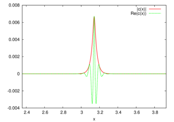
Figure 1: Narrow breather with three crests. $\mbox{Re}(c(x,0))$ and $|c(x,0)|$

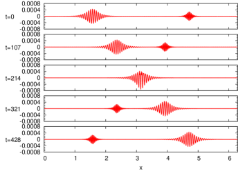
Figure 2: Snapshots of breather collision

6.2 Modulational instability

Freak-wave appearing from homogeneous sea with $k_{0}=100$ and steepness $\mu=0.085$ in the Fig.3:

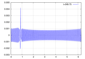
Figure 3: Freak-wave

One can see the beginning of wave breaking in the Fig.4:

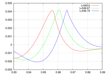
Figure 4: Three snapshots showing beginning of wave breaking

7 Conclusion

We derive new compact and elegant form of Hamiltonian and equation for the gravity waves at the surface of deep water.

• Equation is written for complex normal variable $c(x,t)$ which is analytic function in the upper half-plane

• Hamiltonian both in $k$-space (34) and ix $x$-space (35) is very simple

• Equation itself is very straightforward consisting of only two terms - nonlinear waves and advection

• It can be easily implemented for numerical simulation

The equation can be generalized for ”almost” 2-D waves like KdV is generalized to Kadomtsev-Petviashvili equation:

$$H = \int\!c^{*}\hat{V}c\hskip 2.0ptdxdy+$$ (46)

$$+ \frac{1}{2}\int\!\left[\frac{i}{4}(c^{2}\frac{\partial}{\partial x}{c^{*}}^{2}-{c^{*}}^{2}\frac{\partial}{\partial x}c^{2})-|c|^{2}\hat{K}_{x}(|c|^{2})\right]dxdy$$ (47)

Here operator $\hat{V}$ in K-space is $V_{\vec{k}}=\frac{\omega_{\vec{k}}}{k_{x}}$.

8 Acknowledgments

This work was supported by Grant ”Wave turbulence: theory, numerical simulation, experiment” #14-22-00174 of Russian Science Foundation.

References

• Zakharov (1968) Zakharov, V.E. 1968 Stability of periodic waves of finite amplitude on the surface of a deep fluid, Journal of Applied Mechanics and Technical Physics 9(2), 190–194
• Korotkevich et al (2008) Korotkevich, A.O., Pushkarev, A.N., Resio, D. & Zakharov, V. 2008 Numerical verification of the weak turbulent model for swell evolution, European Journal of Mechanics - B/Fluids 27(4), 361–387
• Crawford et al (1980) Crawford,D.E., Yuen,H.G. and Saffman,P.G. 1980 Evolution of a random inhomogeneous field of nonlinear deep-water gravity waves, Wave Motion , 2(1), 1–16
• Debnath (1994) Debnath, L. 1994 Nonlinear water waves, Academic press Inc.
• Annenkov & Shrira (2011) Annenkov, S.Y. and Shrira, V.I. 2011 Evolution of Wave Turbulence under ”Gusty” Forcing, Phys. Rev. Lett., 107, 114502.
• Annenkov & Shrira (2013) Annenkov, S.Y. and Shrira, V.I. 2013 Large-time evolution of statistical moments of wind-wave fields, Journal of Fluid Mechanics , 726, 517–546.
• Dyachenko & Zakharov (1994) Dyachenko, A.I. and V.E.Zakharov, V.E. 1994 Is free-surface hydrodynamics an integrable system? Phys. Lett. A , 190, 144-148.
• Dyachenko & Zakharov (2011) Dyachenko, A.I. and Zakharov, V.E. 2011 Compact equation for gravity waves on deep water, JETP Letters 93(12), 701–705
• Dyachenko & Zakharov (2012) Dyachenko, A.I., Zakharov, V.E. 2012 A dynamic equation for water waves in one horizontal dimension, European Journal of Mechanics - B/Fluids 32, 17–21
• Fedele & Dutykh (2012) Fedele, F. and Dutykh, D. 2012 Special solutions to a compact equation for deep-water gravity waves, Journal of Fluid Mechanics 712, 646–660
• Fedele & Dutykh (2012a) Fedele, F. and Dutykh, D. 2012 Solitary wave interaction in a compact equation for deep-water gravity waves, JETP Letters 95(12), 622–625
• Dyachenko (2013) Dyachenko,A.I., Kachulin, D.I., Zakharov, V.E. 2013 Collisions of two breathers at the surface of deep water, Nat. Hazards Earth Syst. Sci. 13, 1–6
• Dyachenko et al (2014) Dyachenko A.I., Kachulin D.I. and Zakharov V.E. 2014 Freak waves at the surface of deep water, Journal of Physics: Conference Series 510, 012050
• Fedele (2014a) Fedele, F. 2014 On certain properties of the compact Zakharov equation, Journal of Fluid Mechanics 748, 692–711
• Fedele (2014b) Fedele, F. 2014 On the persistence of breathers at deep water, JETP Letters 98(9), 523–527
• Dyachenko et al (2016) Dyachenko,A.I., Kachulin, D.I., Zakharov, V.E. 2016 Freak-waves: Compact Equation vs Fully Nonlinear One, ”Extreme Ocean Waves” 2nd ed., eds. E. Pelinovsky and C. Harif. Springer, 23-44
• Dyachenko et al (2015a) Dyachenko,A.I., Kachulin, D.I., Zakharov, V.E. 2015 Evolution of one-dimensional wind-driven sea spectra, Pis’ma v ZhETF 102(8), 577–581
• Dyachenko et al (2015b) Dyachenko,A.I., Kachulin, D.I., Zakharov, V.E. 2015 Probability Distribution Functions of freak-waves: nonlinear vs linear model, Stud. in Appl. Math in press
• Dyachenko et al (2013a) Dyachenko, A.I., Kachulin, D.I., Zakharov, V.E. 2013 On the Nonintegrability of the Free Surface Hydrodynamics, JETP. Lett. 98(1), 43–47
• Zakharov (1998) Zakharov, V.E. 1998 Nonlinear waves and wave turbulence, Amer. Math. Soc. Transl. Series 2 182, 167–197
• Zakharov (1999) Zakharov, V.E. 1999 Statistical theory of gravity and capillary waves on the surface of a finite-depth fluid, European Journal of Mechanics - B/Fluids 18(3), 327–344
• Krasitskii (1990) Krasitskii,V.P. Sov. Phys. JETP 71, 921
• Zakharov et al (1992) Zakharov V.E., Lvov V.S. and Falkovich G. 1992 Kolmogorov Spectra of Turbulence I, Springer-Verlag
• Dyachenko et al (1995) Dyachenko A.I., Lvov Y.V. and Zakharov V.E. 1995 Physica D , 87, 233–261.