Investigating some technical improvements to glueball calculations.

Abstract:

We briefly discuss some issues concerning including the pseudoscalar glueball interpolating operators into the variational basis for computing the masses of the $\eta$ and $\eta^{\prime}$ mesons. As a start we present some preliminary results for the correlators from pseudoscalar glueball operators on $n_{f}$ = 2+1+1 twisted mass gauge configurations. Preliminary results for the effect of open boundary conditions on the masses of three glueballs computed in quenched QCD are presented. The statistics of glueball correlators are briefly discussed.

1 Introduction

The glueballs are truly non-perturbative objects in QCD (see [1] for a review of glueballs). We desperately hope they exist in nature, even if they are mixed in with quark degrees of freedom, but, as many Beyond the Standard Model (BSM) experts are finding, experiment may ultimately disappoint us. The quenched glueball spectrum was largely settled over a decade ago [2, 3]. Recent efforts have focused on unquenching the glueball spectrum [4]. Even more recently, it has been speculated, that the $0^{++}$ glueball in some strongly interacting BSM theories is a candidate for a composite Higgs [5, 6].

In this paper we discuss some technical issues in lattice QCD studies of glueball degrees of freedom, as part of our long term goals to find experimental evidence for them and their possible contribution to BSM theories. In this paper we stick with the SU(3) theory.

2 Unquenching the pseuodoscalar glueball

There are a number of challenges with searching for glueball degrees of freedom in nature. Glueball operators will mix with quark operators with the same quantum numbers, so unquenched calculations should include both glueball and quark disconnected diagrams in the same variational calculation. Also high statistics are required. Although large $N_{c}$ arguments suggest that the widths of glueballs should be small, the candidate states which may include glueball degrees of freedom usually have large widths. Hence, specialized resonance techniques are required to study $0^{++}$ states, for example.

It may be easier to consider the pseudo-scalar glueball, even though in the quenched theory the $0^{-+}$ glueball is the third heaviest glueball. The widths of the $\eta$ and $\eta^{\prime}$ mesons are 1.3 kev and 0.2 MeV respectively, hence it is reasonable to neglect resonance effects. Also there are fewer concerns about candidate molecules or tetraquarks as there with the flavour singlet $0^{++}$ hadrons.

Some phenomenologically studies have suggested that in experiment the pseudo-scalar glueball degrees of freedom are at a much lower mass than the quenched pseudo-scalar glueball mass [7]. The few previous lattice studies of unquenching the pseudo-scalar glueball have not seen much difference in the mass at a fixed lattice spacing [4, 8]. However, recently the JLQCD collaboration have used the pseudo-scalar glueball interpolating operators to exact the mass of the $\eta^{\prime}$ meson [9], which suggests a strong mixing of the glueball with the $\eta^{\prime}$.

There has been a big effort to determine the mixing angle between the $\eta$ and $\eta^{\prime}$ meson. For example, the LHCb experiment have recently estimated $\eta$ and $\eta^{\prime}$ mixing [10]. Some $\eta-\eta^{\prime}$ mixing schemes also include the $0^{-+}$ glueball. For example the KLOE experiment [11] wrote the physical $\eta^{\prime}$ meson state in terms of light quarks ($\mid\overline{q}q\rangle$) strange quarks ($\mid\overline{s}s$) and glueball degrees of freedom ($\mid glueball\rangle$).

$$\mid\eta^{\prime}\rangle=X_{\eta^{\prime}}\mid\overline{q}q\rangle+Y_{\eta^{\prime}}\mid\overline{s}s\rangle+Z_{\eta^{\prime}}\mid glueball\rangle$$ (1)

There are different parameterizations of the mixing angles (see [7] for example), but KLOE used one with the constraint $X_{\eta^{\prime}}^{2}+Y_{\eta^{\prime}}^{2}=1$ The KLOE experiment fitted $X_{\eta^{\prime}}$, $Y_{\eta^{\prime}}$, and $Z_{\eta^{\prime}}$ to experimental branching fractions and obtained $Z_{\eta^{\prime}}^{2}=0.14\pm 0.04$.

There have been a number of lattice QCD calculations of $\eta^{\prime}-\eta$ mixing [12, 13, 14, 15, 16]. So it would be good to include the glueball interpolating operators as well, to try to determine $Z_{\eta^{\prime}}$. Although the variational basis used to study $\eta$ and $\eta^{\prime}$ mesons can be extended to include glueball interpolating operators. At this moment, it is less clear to us how to define the quantity $Z_{\eta^{\prime}}$ in terms of lattice QCD correlators. Matrix elements of glueballs have been estimated using quenched QCD [3].

Ensemble	$\beta$	$L^{3}\times T$	$\kappa$	$\mu_{l}$	$\mu_{\sigma}$	$\mu_{\delta}$	No.
D45.32sc	2.10	$32^{3}\times 64$	0.156315	0.0045	0.0937	0.1077	1100
B55.32	1.95	$32^{3}\times 64$	0.161236	0.0055	0.135	0.17	2200
A80.24s	1.90	$24^{3}\times 48$	0.163204	0.008	0.15	0.197	2433

Table 1: Parameters of twisted mass ensembles used in the glueball analysis. Further details are in the papers [17, 18]

We decided to use twisted mass configurations, from the European Twisted Mass collaboration, with $n_{f}=2+1+1$ sea quarks, because these had successfully been used to calculate the mass of the $\eta$ and $\eta^{\prime}$ mesons [16], so we were hopeful that the statistics would be high enough to get a signal with glueball interpolating operators. Three twisted mass ensembles were analyzed using the glueball code developed in [19]. The parameters of the ensembles used are in table 1.

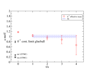
Figure 1: Preliminary effective mass from the $0^{-+}$ glueball interpolating operators from the B45.32sc ensemble. Also included is the continuum limit glueball mass from quenched QCD [3]. Also the masses of the $\eta$ and $\eta^{\prime}$ meson from ETMC [16] from the same ensemble are plotted.

Our glueball code includes an estimate of the projection of the state onto the unphysical toleron state. Unfortunately, the B55.32 ensemble had a very strong projection of the ground state in the pseudo-scalar channel to the toleron. The D45.32sc ensemble had a good overlap of the glueball operator with the ground state in the pseudo-scalar channel. The physical box size of the D45.32sc ensemble was 2.0 fm, compared to 2.5 fm for the B55.32 ensemble. Normally, the contribution of the tolerons is a finite volume effect, so it is not clear why the toleron contribution is larger for the ensemble with the larger physical size. In figure 1 we plot our preliminary results for the effective mass from the $0^{-+}$ glueball operators from the B45.32sc ensemble.

3 Open boundary conditions

One concern about Monte Carlo calculations is that the autocorrelation time is underestimated and the resulting final errors on physical quantities are underestimated, or even worse, there are systematic errors. Different physical quantities have different autocorrelation times. The topological charge is one quantity that has been observed to have large autocorrelation effects which get worse as the continuum limit is taken. Of particular concern are the results from the MILC collaboration [20], where the time series for the topological charge look worse as the lattice spacing is reduced. However, as the MILC collaboration points out, the topological susceptibility from the calculation agrees with theoretical expectations. The two finest lattice spacings simulated by the MILC collaboration are crucial for reducing the errors on phenomenological quantities involving heavy quarks, so it is important to study the issue.

Recently Lüscher and Schaefer have proposed the use of open boundary conditions [21, 22] to improve the sampling of the topological charge. McGlynn and Mawhinney have recently developed a simple model to explain the diffusion of topological charge and compared it to their lattice data [23]. Full QCD calculations with open boundary conditions have already started [24].

What is not clear is whether the large autocorrelation on the topological charge is important for spectral quantities, such as the masses of particles. Chowdhury et al. have recently made a number of studies of the pseudo-scalar [25] and scalar [26] glueballs comparing periodic and open boundary conditions. Within their large errors the glueball masses computed with periodic and open boundary conditions are broadly consistent.

The errors on the mass of the $0^{++}$ glueball by Chowdhury et al. [25, 26] range from 6% to 17%. Given that many high precision lattice QCD calculations quote results at under 1%, then it is desirable to have a more accurate calculation. The calculation of Chowdhury et al. only use one glueball operator (smeared with the Wilson flow) for each channel, so one improvement would be the use of a variational calculation.

$\beta$	$L^{3}\times T$	No.
6.0625	$16^{4}$	11779
6.338	$24^{4}$	4485

Table 2: Parameters of quenched calculation using the Wilson gauge action

In table  2, we report the parameters of the quenched QCD calculations, used to compute the masses of the glueballs with open boundary conditions. The Wilson gauge action was used. The configurations were generated with a standard update algorithm based on an admixture of Cabibbo-Marinari heathbath and over-relaxed sweeps. In this calculation we use a variational calculation, with the code, developed and applied for large $N_{c}$ calculations [19] and unquenched calculations [4]. The use of open boundary conditions means that some of the time slices of correlators have unphysical contributions. In our initial calculations we only used one or two time slices per correlators, rather than average the correlator over all time slices as is normally done for glueball calculation with periodic boundary conditions.

Figure 2: Preliminary results for the masses of the $0^{++}$, $0^{-+}$ and $2^{++}$ glueballs in units of $r_{0}$ computed with open boundary conditions, versus the square of the lattice spacing in units of $r_{0}$. We also include results for the glueball masses from Chowdhury et al. [26, 25] with open boundary conditions. For comparison we include the glueball masses computed with periodic boundary conditions (PBC) by Lucini et al.  [27] and the continuum limit results from Morningstar and Peardon [2].

We use Sommer’s $r_{0}$ parameter to determine the the lattice spacing [28]. Our preliminary results in figure 2 seem to show the the results for glueball masses from open and periodic boundary conditions are consistent, but the errors still need to be reduced for a definite high precision conclusion. The use of the variational code has not reduced the statistical errors over those of Chowdhury et al. [26]. We have probably been too conservative in our choice of time slices to average over. We are currently investigating other options.

4 Statistical distribution of glueball correlators

Calculations which include glueball degrees of freedom require large statistics. One concern is that the probability distribution of the correlators has a “long tail.” This is a potentially generic feature of disconnected diagrams. See for example the modeling of the correlators of the $\eta^{\prime}$ meson in [14].

In some physical calculations, such as the moments in heavy ion collisions, the probability distribution of the data is important [29]. In standard lattice QCD calculations, the law of large numbers makes the underlying distribution of correlators irrelevant, if the statistics are large enough to be in the asymptotic regime. One motivation for studying the statistical distribution of the glueball correlators is the possible use of the techniques developed Endres et al. [30] for many body simulations, where a “filter like procedure” is applied to dramatically reduce the statistical errors.

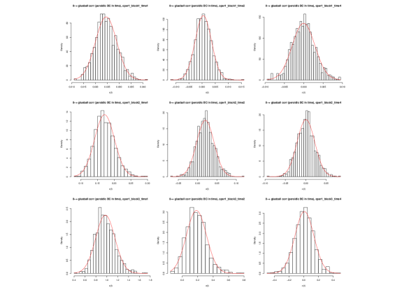
Figure 3: Some $0^{-+}$ glueball correlators, for a specific operator, from the B55.32 twisted mass ensemble. The different graphs are for the time-slices (1 to 3) and blocking levels (1 to 3).

In figure 3 we plot the histograms of some $0^{-+}$ glueball correlators from the B55.32 twisted mass ensemble. Also included is a fit with a Gaussian fit model made with the the R statistical system [31]. The Gaussian distribution gives a good description of the correlator.

5 Conclusions

We have started a project to study whether pseudo-scalar glueball interpolating operators strongly couple to the $\eta^{\prime}$ meson. We have presented preliminary results for the effects of open boundary conditions on the three lightest glueballs.

This work is supported by STFC under the DiRAC framework. We are grateful for the support from the HPCC Plymouth, where part of the numerical computations have been carried out. We thank GridPP and Scotgrid for their support. The ETMC configurations were downloaded from the ILDG [32]. Biagio Lucini is supported by STFC (grant ST/L000369/1) Antonio Rago is supported by the Leverhulme Trust (grant RPG-2014-118) and STFC (grant ST/L000350/1).

References

- [1] V. Mathieu, N. Kochelev, and V. Vento, Int. J. Mod. Phys. E18, 1 (2009), arXiv:0810.4453.
- [2] C. J. Morningstar and M. J. Peardon, Phys. Rev. D60, 034509 (1999), arXiv:hep-lat/9901004.
- [3] Y. Chen et al., Phys. Rev. D73, 014516 (2006), arXiv:hep-lat/0510074.
- [4] E. Gregory et al., JHEP 10, 170 (2012), arXiv:1208.1858.
- [5] J. Kuti, PoS LATTICE2013, 004 (2014).
- [6] Y. Aoki et al., Phys. Rev. D89, 111502 (2014), arXiv:1403.5000.
- [7] H.-Y. Cheng, H.-n. Li, and K.-F. Liu, Phys. Rev. D79, 014024 (2009), arXiv:0811.2577.
- [8] C. M. Richards, A. C. Irving, E. B. Gregory, and C. McNeile, Phys. Rev. D82, 034501 (2010), arXiv:1005.2473.
- [9] H. Fukaya et al., (2015), arXiv:1509.00944.
- [10] R. Aaij et al., JHEP 01, 024 (2015), arXiv:1411.0943.
- [11] F. Ambrosino et al., Phys. Lett. B648, 267 (2007), arXiv:hep-ex/0612029.
- [12] C. McNeile and C. Michael, Phys. Lett. B491, 123 (2000), arXiv:hep-lat/0006020, [Erratum: Phys. Lett.B551,391(2003)].
- [13] N. H. Christ et al., Phys. Rev. Lett. 105, 241601 (2010), arXiv:1002.2999.
- [14] E. B. Gregory, A. C. Irving, C. M. Richards, and C. McNeile, Phys. Rev. D86, 014504 (2012), arXiv:1112.4384.
- [15] J. J. Dudek, R. G. Edwards, P. Guo, and C. E. Thomas, Phys. Rev. D88, 094505 (2013), arXiv:1309.2608.
- [16] C. Michael, K. Ottnad, and C. Urbach, Phys. Rev. Lett. 111, 181602 (2013), arXiv:1310.1207.
- [17] R. Baron et al., JHEP 06, 111 (2010), arXiv:1004.5284.
- [18] C. Michael, K. Ottnad, and C. Urbach, PoS LATTICE2013, 253 (2014), arXiv:1311.5490.
- [19] B. Lucini, A. Rago, and E. Rinaldi, JHEP 08, 119 (2010), arXiv:1007.3879.
- [20] A. Bazavov et al., Phys. Rev. D87, 054505 (2013), arXiv:1212.4768.
- [21] M. Luscher and S. Schaefer, JHEP 07, 036 (2011), arXiv:1105.4749.
- [22] M. Luscher and S. Schaefer, Comput. Phys. Commun. 184, 519 (2013), arXiv:1206.2809.
- [23] G. McGlynn and R. D. Mawhinney, Phys. Rev. D90, 074502 (2014), arXiv:1406.4551.
- [24] W. Soldner, PoS LATTICE2014, 099 (2015), arXiv:1502.05481.
- [25] A. Chowdhury, A. Harindranath, and J. Maiti, Phys. Rev. D91, 074507 (2015), arXiv:1409.6459.
- [26] A. Chowdhury, A. Harindranath, and J. Maiti, JHEP 06, 067 (2014), arXiv:1402.7138.
- [27] B. Lucini, M. Teper, and U. Wenger, JHEP 06, 012 (2004), arXiv:hep-lat/0404008.
- [28] R. Sommer, Nucl. Phys. B411, 839 (1994), arXiv:hep-lat/9310022.
- [29] L. Chen, Z. Li, X. Zhong, Y. He, and Y. Wu, J. Phys. G42, 065103 (2015), arXiv:1504.04445.
- [30] M. G. Endres, D. B. Kaplan, J.-W. Lee, and A. N. Nicholson, PoS LATTICE2011, 017 (2011), arXiv:1112.4023.
- [31] R Core Team, R: A Language and Environment for Statistical Computing, R Foundation for Statistical Computing, Vienna, Austria, 2014.
- [32] M. G. Beckett et al., Comput. Phys. Commun. 182, 1208 (2011), arXiv:0910.1692.