Influence diagrams for the optimization of a vehicle speed profile

Abstract

Influence diagrams are decision theoretic extensions of Bayesian networks. They are applied to diverse decision problems. In this paper we apply influence diagrams to the optimization of a vehicle speed profile. We present results of computational experiments in which an influence diagram was used to optimize the speed profile of a Formula 1 race car at the Silverstone F1 circuit. The computed lap time and speed profiles correspond well to those achieved by test pilots. An extended version of our model that considers a more complex optimization function and diverse traffic constraints is currently being tested onboard a testing car by a major car manufacturer. This paper opens doors for new applications of influence diagrams.

1 INTRODUCTION

Optimization of a vehicle speed profile is a well known problem studied in literature. Some authors minimize the energy consumption (Monastyrsky and Golownykh,, 1993; Chang and Morlok,, 2005; Saboohi and Farzaneh,, 2009; Hellström et al.,, 2010; Mensing et al.,, 2011; Rakha et al.,, 2012) while others aim at minimizing the total time (Velenis and Tsiotras,, 2008).

In this paper we describe an application of influence diagrams to the problem of the optimization of a vehicle speed profile. Speed profile specifies the vehicle speed at each point of the path. We illustrate the proposed method using an example of the speed profile optimization of a Formula 1 race car at the Silverstone F1 circuit (Velenis and Tsiotras,, 2008). The goal is to minimize the total lap time. This example will be used throughout the paper to explain the key concepts and for the final experimental evaluation of the proposed approach. An advantage is that the optimal solution is known (Velenis and Tsiotras,, 2008). This allows us to compare the influence diagram solution with the analytic one. Both solutions have a close correspondence.

The proposed method allows applications of influence diagrams to more complex scenarios of a speed profile optimization. Speed constraints can be invoked not only by path radii, but also by other causes like traffic regulations, weather conditions, distance to other vehicles, etc. Moreover, these conditions can be changing dynamically. Also, the criteria to be optimized need not be the total time only. We can consider also safety, fuel consumption, etc. We believe that influence diagrams are very appropriate for these situations since optimum policies are precomputed for any speed the vehicle can attain. The optimal speed profile can be quickly updated if the conditions change.

There are two key properties that allow efficient computations. The first one is that the overall utility function is the sum of local utilities in all considered segments of the vehicle path. This is the case not only when the goal is to minimize the total time, but also when we aim at the minimal total fuel consumption or a linear combination of these two. The second key property is the Markov property. This allows to aggregate the whole future in one probability and one utility potential. These potentials are defined over the speed variable in the current path segment.

The paper is organized as follows. In Section 2, we describe the physical model of a vehicle and define the problem of the vehicle speed profile optimization. In Section 3, we introduce influence diagrams and in Section 4 we apply them to the vehicle speed profile optimization. The results of numerical experiments with real data are presented in Section 5. Section 6 reviews the related work. In Section 7, we conclude the paper by a summary of our contribution and by a discussion of our future work.

2 PHYSICAL MODEL OF THE VEHICLE

First, we describe a simple physical model of a vehicle. The content of this section is based on (Velenis and Tsiotras,, 2008). Although this model is too simple to model the complex behavior of a car-like vehicle, it is sufficient for the optimization of a vehicle speed profile.

Figure 1: A point mass moving along a path.

We model a vehicle as a point mass moving along a path, see Figure 1. We split the path into $n\in\mathbb{N}$ small segments of a specified length (e.g., $5$ meters). Let $s$ denote the length of each segment, $i\in\{0,\ldots,n\}$ be the path length coordinate, $[i,i+1]$ be the segment between path length coordinates $i$ and $i+1$. We assume that the acceleration is constant at each segment. Let $v_{i}$ be the velocity at $i$, and $a_{i}$ the acceleration at the segment $[i,i+1]$. The velocity $v_{i+1}$ at $i+1$ is a function of the velocity $v_{i}$ and acceleration $a_{i}$:

$$v_{i+1} = v_{i+1}(v_{i},a_{i},s)\ \ =\ \ \sqrt{(v_{i})^{2}+2\cdot s\cdot a_{i}}\enspace.\rule{11.38109pt}{0.0pt}$$ (1)

Time $t_{i+1}$ spent at the path segment $[i,i+1]$ is:

$$t_{i+1} = t_{i+1}(v_{i},v_{i+1},s)\ \ =\ \ s\cdot\left({\frac{v_{i}+v_{i+1}}{2}}\right)^{-1}.\rule{11.38109pt}{0.0pt}$$ (2)

The vehicle is controlled by a control variable $u_{i}$, which is assumed to be constant at the segment $[i,i+1]$. The control variable $u_{i}$ takes values from interval $[-1,+1]$, where negative values represent braking and positive values represent accelerating. We use variable $u_{i}$ to control acceleration $a_{i}$:

$$a_{i} = \left\{\begin{array}[]{ll}a_{t}^{max}\cdot u_{i}-c_{v}\cdot(v_{i})^{2}&\mbox{if $u_{i}\geq 0$}\\ a_{t}^{min}\cdot u_{i}-c_{v}\cdot(v_{i})^{2}&\mbox{if $u_{i}<0$ \ ,}\end{array}\right.$$ (5)

where $a_{t}^{max}$ and $a_{t}^{min}$ are engine and brakes characteristics, namely the maximum tangential acceleration and deceleration, respectively. $c_{v}$ is the deceleration coefficient for aerodynamic drag.

Example 1.

For a F1 race car:

$$a_{i}\ \ =\ \ a_{i}(u_{i},v_{i})$$ (8)

$$= \left\{\begin{array}[]{ll}16\cdot u_{i}-0.0021\cdot(v_{i})^{2}&\mbox{if $u_{i}\geq 0$}\\ 18\cdot u_{i}-0.0021\cdot(v_{i})^{2}&\mbox{if $u_{i}<0$ \ .}\end{array}\right.$$

The vehicle path is characterized by a radius profile, which is defined as the radius $r_{i}$ of the circular arc which best approximates the path curve at each point $i=1,\ldots,n$ (see Figure 1). The radius $r_{i}$ defines the maximum speed at point $i$ as

$$v_{i} \leq v_{i}^{max}\ \ =\ \ \sqrt{a_{n}^{max}\cdot r_{i}}\enspace,$$ (9)

where $a_{n}^{max}$ is the maximum lateral acceleration.

Example 2.

For a typical F1 race car $a_{n}^{max}=30\ m\cdot s^{-2}$. This implies that

$$v_{i}^{max} = \sqrt{30\cdot r_{i}\enspace}\enspace.$$ (10)

If $r_{i}=30\ m$ then the maximum speed is $108\ km\cdot h^{-1}$.

Example 3.

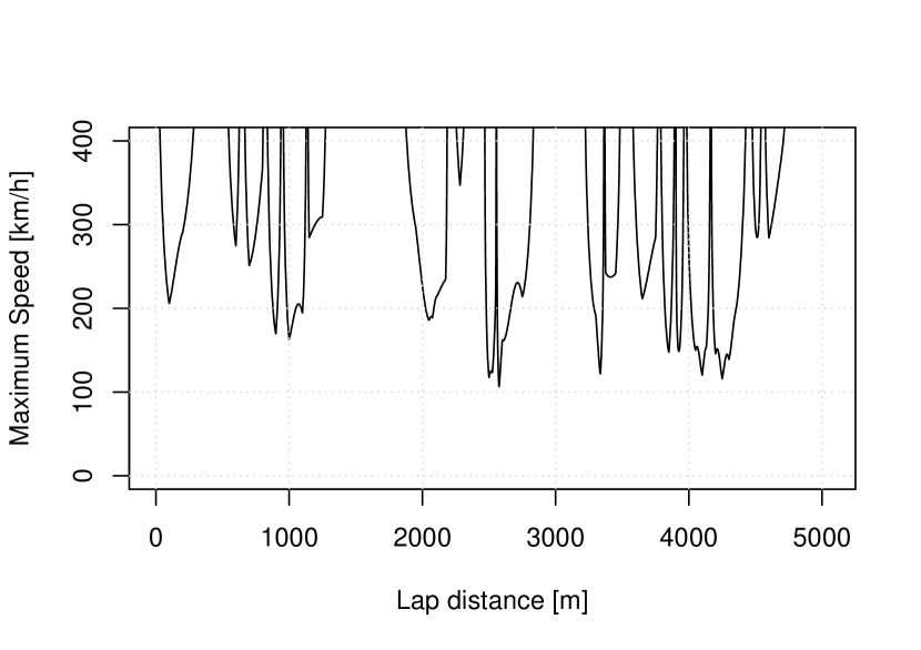
In Figure 2, we present the radius and maximum speed profiles of the F1 Silverstone circuit (the bridge version). The radius larger than $500$ meters is not depicted. From the radius profile, we derive the maximum speed profile by use of formula (10).

Figure 2: Radius and maximum speed profiles.

Other restrictions on maximal and minimal tangential accelerations are due to friction forces at the tires, which restricts the control signals:

$$|u_{i}| \leq u_{i}^{max}(v_{i})\ \ =\ \ \sqrt{1-\left(\frac{v_{i}}{v_{i}^{max}}\right)^{4}}\enspace.$$ (11)

Now, we can formally specify the problem.

Definition 1 (Vehicle speed profile optimization problem).

The goal is to find a vehicle speed profile $v_{i},i=1,\ldots,n$ such that

• $v_{0}$ is the actual speed of the vehicle at coordinate $0$,

• it minimizes the total time $\sum_{i=1}^{n}t_{i}$,

• it satisfies the speed constraints specified by formula (9) for $i=0,1,\ldots,n$ and

• it satisfies the control constraints specified by formula (11) for $i=0,1,\ldots,n$.

Remark.

Please, note that an optimal speed profile can be also specified by values of control variable $u_{i}$ for $i=0,\ldots,n-1$, from which it is computed.

3 INFLUENCE DIAGRAMS

An influence diagram (Howard and Matheson,, 1981) is a Bayesian network augmented with decision variables and utility functions. In graphs, random variables are depicted as circles, decision variables as squares, and utility functions as diamonds. As an example, see Figure 3. Random and decision variables are denoted by capital letters, their states by respective lower-case ones.

A solution to the decision problem described by an influence diagram consists of a series of decision policies for the decision variables. Decision policy for decision variable $U$ defines for each configuration of parents of $U$ a probability distribution over the states of $U$. Decision strategy is a sequence of decision policies, one for every decision variable. The goal is to find an optimal decision strategy that maximizes the expected total utility.

3.1 SOLVING INFLUENCE DIAGRAMS

Several methods for solving influence diagrams were proposed. A simple method was published already in (Howard and Matheson,, 1981) where influence diagrams were introduced. They proposed to unfold respective influence diagram into a decision tree and solve it using dynamic programming. Another algorithm was developed by (Shachter,, 1986) and it foreshadowed the future graphical algorithms. Basically, one can gradually simplify respective influence diagram by successive removing nodes from its graph. When a decision node is being removed (by maximizing expected utility), the maximizing alternative is recorded as the optimal policy. Three operations to remove graph nodes were introduced; at least one of them can be used at any given time. Another method is to reduce an influence diagram into a Bayesian network by converting decision variables into random variables – the solution of a specific inference problem in this Bayesian network then corresponds to the optimal decision policy of the influence diagram (Cooper,, 1988). One can also transform an influence diagram into a valuation network and solve it using variable elimination in the valuation network (Shenoy,, 1992).

We decided to use a method that employs a strong junction tree (Jensen et al.,, 1994; Jensen and Nielsen,, 2007), which is a refinement of methods of Shenoy, (1992) and Shachter and Peot, (1992). The utility nodes are eliminated first by marrying all parents of each utility node and by including the corresponding utility potentials to cliques containing all parents of the utility node. It has been shown that an influence diagram can be solved exactly by message passing performed on the strong junction tree.

To every clique $C$ in the junction tree, we associate a probability potential $\Phi_{C}$ and a utility potential $\Psi_{C}$. Let $C_{1}$ and $C_{2}$ be adjacent cliques with separator $S$. To pass a message from clique $C_{2}$ to clique $C_{1}$ potentials $\Phi_{C_{1}}$ and $\Psi_{C_{1}}$ are updated as follows (Jensen et al.,, 1994):

$$\Phi^{\prime}_{C_{1}} = \Phi_{C_{1}}*\Phi_{S},$$ (12)

$$\Psi^{\prime}_{C_{1}} = \Psi_{C_{1}}+\frac{\Psi_{S}}{\Phi_{S}}\enspace,$$ (13)

where

$$\Phi_{S}\ =\ \underset{C_{2}\setminus S}{\mathcal{M}}\Phi_{C_{2}}, \Psi_{S}\ =\ \underset{C_{2}\setminus S}{\mathcal{M}}\left(\Phi_{C_{2}}*\Psi_{C_{2}}\right)$$

and $\mathcal{M}$ is a generalized marginalization operation. The operator $\mathcal{M}$ acts differently for a random variable $A$ and a decision variable $U$ of a (probability or utility) potential $\Xi$:

$$\underset{A}{\mathcal{M}}\Xi=\sum_{A}\Xi,~{}~{}~{}~{}~{}\underset{U}{\mathcal{M}}\Xi=\max_{U}\Xi\enspace,$$

where $\sum_{A}$ is a shorthand for summation over all states of $A$ and $\max_{U}$ denotes maximum over all states of $U$. For a set of variables $C$, we define $\mathcal{M}_{C}\Xi$ as a sequence of single-variable marginalizations. The elimination order follows the inverse order as determined by the relation $\prec$. In case of discrete variables, the complexity of one message passing operation is $O(|C_{1}|+|C_{2}|+|S|)$, where $|C|$ denotes the number of combinations of states of variables in $C$.

Despite its similarity with the junction tree algorithm for Bayesian networks (Lauritzen and Spiegelhalter,, 1988), only the collection phase of the strong junction tree is needed to solve an influence diagram. The maximum expected utility value can be obtained by doing the remaining marginalization in the root. Above that, we can easily get the optimal decision policy for decision variables during the message passing process. For every combination of parents of a decision variable (in our case the only parent is the speed variable), it is the alternative with the maximal expected utility in the moment of message passing.

Note that this approach is highly dependent on the process of building a junction tree from an influence diagram. The size of cliques is determining the speed of the algorithm. Consequently, the junction tree algorithm is typically infeasible for solving large influence diagrams. Fortunately, this is not the case for our application.

4 INFLUENCE DIAGRAMS FOR VEHICLE SPEED PROFILE OPTIMIZATION

In this section, we use the physical model of a vehicle from Section 2 to create an influence diagram for the speed profile optimization. We split the vehicle path into $n$ segments of the same length $s$. In each segment $[i,i+1]$, $i\in\{0,\ldots,n-1\}$ there are three random variables $V_{i},A_{i},$ and $V_{i+1}$, one decision variable $U_{i}$, and one utility potential $T_{i}$. A part of influence diagram corresponding to one path segment is depicted in Figure 3. The influence diagram used in the final experiments reported in Section 5 consisted of $1010$ parts, one for a segment 5 meters long.

Figure 3: A part of influence diagram corresponding to the path segment $[i,i+1]$.

Variable $V_{i}$ corresponds to the vehicle speed in the beginning of the segment (at point $i$). $A_{i}$ corresponds to the vehicle acceleration in the segment $[i,i+1]$ and it is assumed to be constant in this segment. $V_{i+1}$ is the vehicle speed at the end of the segment (at point $i+1$). The decision variable $U_{i}$ corresponds to the vehicle control signal whose positive values denote application of vehicle accelerator and negative values ones an application of brakes. Utility function $T_{i}$ corresponds to time spent at segment $[i,i+1]$. In our implementation the actual values of $T_{i}$ are time savings achieved at segment $[i,i+1]$. They are computed by subtracting time spent by the vehicle in the segment from a constant $t^{max}$ – the maximum considered time the vehicle may spend at a segment of length $s$. This allows us to use maximization over non-negative utility potentials, which is required when working with random variables having states of zero probability.

In this paper we consider discrete random and discrete decision variables. For all $i\in\{0,\ldots,n\}$, the variable $V_{i}$ takes its values from $\mathcal{V}$, which is a finite subset of interval $[0,400]$ measured in $km/h$, the values of $A_{i}$ are from $\mathcal{A}$, which is a finite subset of interval $[-34,16]$ measured in $ms^{-2}$, and values of decision variable $U_{i}$ are from $\mathcal{U}$, which is a finite subset of interval $[-100,+100]$, where value $-100$ corresponds to the maximum braking (brakes $100\%$) while $+100$ corresponds to full acceleration (accelerator $100\%$). Sets $\mathcal{V}$, $\mathcal{A}$, and $\mathcal{U}$ are uniformly discretized with discretization steps $d_{V}$, $d_{A}$, and $d_{U}$, respectively. Symbols $|\mathcal{V}|$, $|\mathcal{A}|$, and $|\mathcal{U}|$ denote the cardinalities of the respective sets.

The probability and utility potentials are defined using formulas from Section 2. The conditional probability distributions are “almost” deterministic. For each parent configuration of a variable there are only two states from the finite domain of that variable with a non-zero probability. These two values are those that are closest to the value computed by the corresponding formula of the physical model of the vehicle. The conditional probability distribution of the acceleration $A_{i}$ is defined as:

$$P(A_{i}=a|V_{i}=v_{i},U_{i}=u_{i})\ \ =$$ (17)

$$\left\{\begin{array}[]{ll}1-\frac{a_{i}-a}{d_{A}}&\mbox{if $a=\max\{a\in\mathcal{A},a\leq a_{i}\}$}\\[2.84526pt] 1-\frac{a-a_{i}}{d_{A}}&\mbox{if $a=\min\{a\in\mathcal{A},a>a_{i}\}$}\\ 0&\mbox{otherwise,}\end{array}\right.\rule{8.53581pt}{0.0pt}$$

where $a_{i}$ is defined by formula (5).

Example 4.

Consider $P(A_{i}|V_{i}=131km/h,U_{i}=25)$ and $\mathcal{A}=\{-34,-33,\ldots,-1,0,1,2,\ldots,16\}$. Using (8) we compute the acceleration of an F1 race car $a_{i}=1.2\ ms^{-2}$. The conditional probability distribution is specified in Table 1.

Table 1: The conditional probability table $P(A_{i}|V_{i}=131km/h,U_{i}=25)$

$a_{i}$	…	-1	0	1	2	3	…
$P(a_{i}|v_{i},u_{i})$	0	0	0	0.8	0.2	0	0

Similarly, we define the conditional probability distribution $P(V_{i+1}|V_{i},A_{i})$. More specifically, we combine the above approximation and formula (1). Finally, the utility function is defined as

$$f(v_{i-1},v_{i},s) = t^{max}-t_{i}(v_{i-1},v_{i},s)\enspace,\rule{14.22636pt}{0.0pt}$$ (18)

where function $t_{i}$ is defined by formula (2).

After elimination of utility nodes, the graph of the influence diagram is transformed into a strong junction tree. See Figure 4 where we present the strong junction tree of influence diagram from Figure 3. There are two cliques for path segment $[i,i+1]$, $i\in\{0,\ldots,n-1\}$ in the strong junction tree. We will denote them $C_{i}^{A}$ and $C_{i}^{V}$ and define $C_{i}^{A}=\{A_{i},U_{i},V_{i}\}$ and $C_{i}^{V}=\{V_{i+1},A_{i},V_{i}\}$. Cliques are ordered reversely and the variable elimination is processed also in this order. Rectangular nodes correspond to junction tree separators.

Figure 4: The strong junction tree for the part of influence diagram from Figure 3.

The junction tree is initialized as follows. Each conditional probability distribution and each utility function is assigned to a clique containing all its variables. Thus

$$\begin{array}[]{ll}\Phi_{C_{i}^{A}}\ =\ P(A_{i}|U_{i},V_{i})\enspace,&\Phi_{C_{i}^{V}}\ =\ P(V_{i+1}|A_{i},V_{i})\enspace,\\ \Psi_{C_{i}^{A}}\ =\ 0\enspace,&\Psi_{C_{i}^{V}}\ =\ f(T_{i+1}|V_{i},V_{i+1})\enspace.\end{array}$$

4.1 IMPLEMENTATION OF CONSTRAINTS

During the inference we have to consider the speed and control constraints. Both, speed and control constraints are inserted to corresponding cliques of the junction tree.

4.1.1 Speed constraints

Speed constraints are inserted in the form of likelihood evidence. Likelihood evidence is a vector that for each state of the corresponding variable takes values between zero and one (Jensen,, 2001, Section 1.4.6). Likelihood evidence of a speed constraint is a vector $\phi$ of length $|\mathcal{V}|$ such that

$$\phi(v)\ \ =$$ (22)

$$\left\{\begin{array}[]{ll}1&\mbox{if $v\leq v_{i}^{max}$}\\ 1-\frac{v-v_{i}^{max}}{d_{V}}&\mbox{if $v=\min\{v\in\mathcal{V},v>v_{i}^{max}\}$}\rule{14.22636pt}{0.0pt}\\ 0&\mbox{otherwise,}\end{array}\right.$$

where $v_{i}^{max}$ is defined by (9).

Remark.

The idea behind the formula (22) is that the closer the value of $v_{i}^{max}$ is to the nearest speed value $v\in\mathcal{V}$ that is greater than $v_{i}^{max}$ the higher is the likelihood of $v$. In experiments, we observed that by giving a non-zero probability to the state $v$ just above the maximum value $v_{i}^{max}$ we improve the quality of results. The coarser the discretization the larger the improvement.

During the inference we include potential $\phi(V_{i})$ into a clique containing $V_{i}$ that appears first in the computations.

4.1.2 Control constraints

The control constraints (11) are applied during marginalization of the control variable $U_{i}$ from a potential $\Psi_{C_{i}^{V}}^{\prime}$ (we will abbreviate it as $\Xi$) performed in the steps specified by formulas (12) and (13).

For each $v_{i}\in\mathcal{V}$ we define a set of admissible control

$$\mathcal{U}^{\prime}(v_{i}) = \{u_{i}\in\mathcal{U},|u_{i}|\leq u_{i}^{max}(v_{i})\}$$

and compute an optimal admissible control value

$$u_{i}^{*}(v_{i}) = \arg\max_{u_{i}\in\mathcal{U}^{\prime}(v_{i})}\Xi(U_{i}=u_{i},V_{i}=v_{i})\enspace.$$

The optimal decision policy in $U_{i}$ is for all $v_{i}\in\mathcal{V}$

$$\delta_{i}(u|v_{i}) = \left\{\begin{array}[]{ll}1&\mbox{if $u=u_{i}^{*}(v_{i})$}\\ 0&\mbox{otherwise.}\end{array}\right.$$ (25)

The value of the new potential is

$$\Xi(V_{i}=v_{i}) = \Xi(U_{i}=u_{i}^{*}(v_{i}),V_{i}=v_{i})\enspace.$$ (26)

However, whenever $u_{i}^{*}(v_{i})$ is the least or the largest value of $\mathcal{U}^{\prime}(v_{i})$ we can reduce the discretization error by considering also the nearest value $u_{i}^{**}(v_{i})$ outside $\mathcal{U}^{\prime}_{i}$. The idea is similar to (22). If

$$\Xi(U_{i}=u_{i}^{**}(v_{i}),V_{i}=v_{i}) \geq \Xi(U_{i}=u_{i}^{*}(v_{i}),V_{i}=v_{i})$$

then we replace the deterministic policy (25) by a probabilistic policy

$$\delta_{i}(u|v_{i}) = \left\{\begin{array}[]{ll}1-\frac{|u_{i}^{*}(v_{i})-u_{i}^{max}(v_{i})|}{d_{U}}&\mbox{if $u=u_{i}^{*}(v_{i})$}\\ 1-\frac{|u_{i}^{**}(v_{i})-u_{i}^{max}(v_{i})|}{d_{U}}&\mbox{if $u=u_{i}^{**}(v_{i})$}\\ 0&\mbox{otherwise.}\end{array}\right.$$

Formula (26) is replaced by

$$\Xi(V_{i}=v_{i})\ \ =$$

$$\delta_{i}(u_{i}^{*}|v_{i})\cdot\Xi(U_{i}=u^{*}(v_{i}),V_{i}=v_{i})$$

$$+\delta_{i}(u_{i}^{**}|v_{i})\cdot\Xi(U_{i}=u_{i}^{**}(v_{i}),V_{i}=v_{i})\enspace.$$

4.2 ZERO COMPRESSION

We solve the influence method using standard strong junction tree method (Jensen et al.,, 1994) briefly described in Section 3.1. But the probability potentials we are working with are sparse, i.e., they contain many zeroes. This is a consequence of conditional probability distributions being “almost” deterministic. In Hugin (Andersen et al.,, 1990) a procedure called zero compression is employed to improve efficiency of inference with sparse potentials. In this procedure an efficient representation of the clique tables is used so that zeros need not be stored explicitly. The savings can be large: in our case, we basically reduce the dimension of each table by one. The compression does not affect the accuracy of the inference process, as it introduces no approximations (Cowell et al.,, 1999), i.e., it is an exact inference method.

Example 5.

We can store the distribution from Example 4 using two numbers only – value $val$ and position $pos$ of the first non-zero number in the table. Note that the second non-zero number is positioned on $pos+1$ with value $1-val$ and there are two non-zero numbers only. The same applies to $P(V_{i+1}|V_{i},A_{i})$.

In the standard inference method the complexity in one path segment is $O\left(|\mathcal{A}|\cdot|\mathcal{V}|\cdot(|\mathcal{V}|+|\mathcal{U}|)\right)$. In case of zero compression the complexity drops to $O(|\mathcal{V}|\cdot(|\mathcal{A}|+|\mathcal{U}|))$. In Section 5.1 we evaluate the savings experimentally.

5 EXPERIMENTS

We performed experiments with a model of a Formula 1 race car at the Silverstone F1 circuit (the bridge version). The goal is to find a speed profile that minimizes the total lap time and satisfies speed and acceleration constraints as specified by Definition 1. The speed constraints are derived from radius of curves and the maximum allowed lateral acceleration $a_{n}^{max}$ – see formula (9). For a typical F1 race car $a_{n}^{max}=30\ ms^{-2}$ – see Example 2. The acceleration constraints are defined by formula (11).

In our experiments we use the influence diagram described in Section 3. The experiments were conducted in the following way:

1. Define the length of one segment $s$ and sets of variables’ states $\mathcal{V,A,U}$.

2. Initialize potentials $\Phi_{C_{i}^{A}},\Phi_{C_{i}^{V}},\Psi_{C_{i}^{A}},$ and $\Psi_{C_{i}^{V}}$ and set up the junction tree.

3. Insert speed and acceleration constraints to the junction tree.

4. Compute the optimal policies $\delta_{i},i=0,1,\ldots,n-1$.

5. Use the optimal policy and the initial speed $v_{0}=312\ km/h$ to compute an optimal speed profile as specified by formulas (28), (29), and (30).

The expected speed $\hat{v}_{i+1}$ at coordinate $i+1$ is computed using formulas (1) and (8) from the expected control value $\hat{u}_{i}(v_{i})$, which is computed as a weighted average of policies for two values $\underline{v}_{i},\overline{v}_{i}$ from $\mathcal{V}$ that are the closest to $v_{i}$:

$$\hat{v}_{i+1} = v_{i+1}(v,s,a_{i}\left(\hat{u}_{i}(v_{i}),v_{i})\right)\enspace,$$ (28)

$$\hat{u}_{i}(v_{i}) = \sum_{v\in\{\underline{v}_{i},\overline{v}_{i}\}}w(v,v_{i})\cdot\sum_{u\in\mathcal{U}}u\cdot\delta_{i}(u|v)\enspace,\rule{14.22636pt}{0.0pt}$$ (29)

$$w(v,v_{i}) = 1-\frac{|v-v_{i}|}{d_{V}}\enspace.$$ (30)

All algorithms used in our experiments were implemented in the programming language R (R Core Team,, 2014).

5.1 ZERO COMPRESSION EXPERIMENTS

We compared computational time of the zero compression and standard junction tree inference methods, see Table 2. Recall that symbols $|\mathcal{V}|$, $|\mathcal{A}|$, and $|\mathcal{U}|$ denote the cardinalities of the respective sets. The experiments were carried out on an influence diagram consisting of 10 path segments. We can see that zero compression brings large computational savings for fine grained discretizations.

Table 2: Comparisons of the CPU time for the zero compression and the standard approach.

$|\mathcal{V}|$	$|\mathcal{A}|$	$|\mathcal{U}|$	zero compr. $[s]$	standard $[s]$
50	50	50	0.08	0.73
100	100	100	0.20	4.78
100	100	200	0.19	7.09
100	200	100	0.25	9.17
200	100	100	0.39	13.01
200	200	100	0.49	24.30
200	200	200	0.50	29.61
400	100	100	0.84	38.53
400	400	100	1.26	142.92

5.2 DISCRETIZATION EXPERIMENTS

We tested different variable discretizations and different path segmentations. The goal was to find a combination of these parameters that represents a reasonable tradeoff between precision and computational time.

Settings: $s=1m$, $\mathcal{|V|=|A|=|U|}=100$	Settings: $s=5m$, $\mathcal{|V|=|A|=|U|}=100$
Settings: $s=1m$, $|\mathcal{V}|=400,\mathcal{|A|=|U|}=100$	Settings: $s=5m$, $|\mathcal{V}|=400,\mathcal{|A|=|U|}=100$

Figure 5: Comparisons of various path segmentations and discretizations.

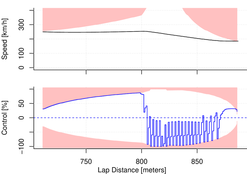
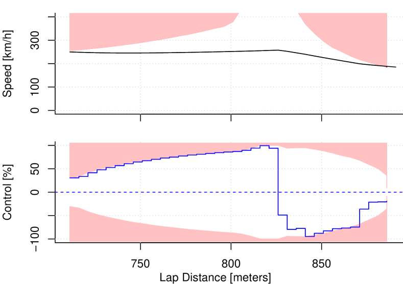
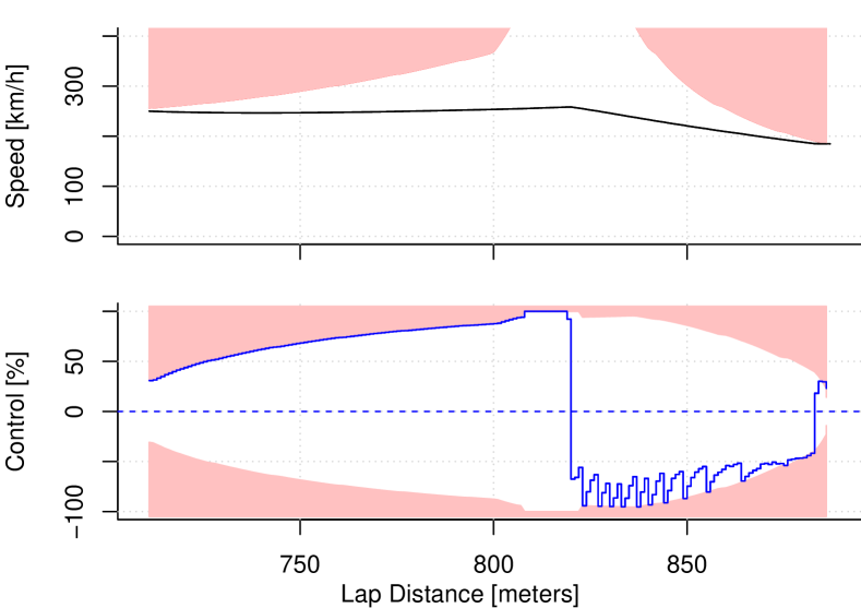
We performed experiments on a part of Silverstone F1 circuit 180 meters long. Results of some performed experiments are presented in Figure 5. In the upper part of these figures, speed profiles are depicted while the control profile is plotted in their lower part. The shaded areas are forbidden by the speed and control constraints, respectively.

It turned out that the number of states of the model variables should be in accordance with the path segmentation. The finer is the path segmentation, the more variables’ values are required. Discretization that is not well balanced with the path segmentation leads to oscillations of decision (control) variables as it is illustrated for $s=1m$, $\mathcal{|V|=|A|=|U|}=100$ in Figure 5.

In the experiments it turned out the oscillation depends strongly on $|\mathcal{V}|$. Basically, there are two reasons. First, the discretization has to be able to distinguish small speed changes within one segment of the path. The reason can be elucidated by the following example.

Example 6.

Consider uniformly accelerated motion with the initial speed $v_{0}\in\{200\ km/h,300\ km/h\}$. In case of full throttle, the acceleration computed by formula (8) is $a\doteq 9.52\ ms^{-2}$ and $a\doteq 1.42\ ms^{-2}$, respectively. Considering segments of various length $s$, we can compute the speed at the end of the respective segment using formula (1). From Table 3 we can see that in case of $s=1\ m$ the discretization has to be fine grained in order to capture small speed changes within such a short segment.

Table 3: Speed [in $km/h$] in case of full acceleration

$v_{0}$	$v_{1}$
	$s=1\ m$	$s=5\ m$	$s=20\ m$
200	200.6159	203.0606	211.9774
300	300.0612	300.3058	301.2215

The second reason is the inference algorithm itself. Information passes through clique separators. In Figure 4 we can see that all separators contain $V_{i}$ and every second separator consists of single $V_{i}$ only. Hence, the size of $\mathcal{V}$ limits the information flow between respective cliques. In other words, $|\mathcal{V}|$ represents a bottleneck of the inference mechanism.

Representative results for the whole Silverstone F1 circuit are presented in Table 4. The expected lap time is quite stable with respect to different discretizations. For the final experiments we selected the configuration printed in boldface since from those that respect the speed and acceleration constraints well it is least computationally demanding.

Table 4: CPU and lap time for diverse path segmentations and discretizations.

$s$	$\mathcal{|V|}$	$\mathcal{|A|}$	$\mathcal{|U|}$	lap time	CPU time
$[m]$				$[s]$	$[s]$
10	400	200	100	83.92	20.61
10	800	400	200	83.83	103.94
5	400	200	100	84.09	42.88
5	800	200	100	83.97	166.88
5	800	400	200	83.95	197.93
5	800	800	800	83.94	473.16
5	1000	1000	1000	83.91	588.80
1	800	400	200	84.17	2110.68
1	1000	1000	1000	84.10	2850.66
1	1600	1000	1000	83.96	5544.99

5.3 INFLUENCE DIAGRAM SOLUTION

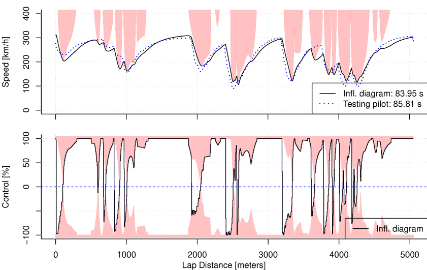
We used the influence diagram to compute the speed profile for the Silverstone F1 circuit. It is plotted in the upper part of Figure 6 by a full line. The bridge version of Silverstone circuit is $5049$ meters long, which corresponds to $1010$ segments $5m$ long. In this figure we compare the computed speed profile with a test pilot performance at the Silverstone F1 circuit (Oxford Technical Solutions,, 2002). In the upper part of Figure 6 the test pilot speed profile is plotted by a dotted line. Notice that the testing pilot violates these restrictions several times. Also, the test pilot acceleration is slower than expected. The speed constraints used in the model seem to be too cautious and the car acceleration ability a bit exaggerated.

It is interesting to compare the total lap time estimated by the influence diagram model with results achieved by F1 pilots. While the model estimated time $83.95$ seconds is little lower than time achieved by the test pilot – $85.51$ seconds, it is higher than the fastest ever lap time – $78.12$ seconds – attained by Sebastian Vettel with his Red Bull-Renault in the qualification of the 2009 British Grand Prix.

Figure 6: A comparison of speed profiles: the influence diagram and a test pilot (Oxford Technical Solutions,, 2002). The shaded areas are forbidden by the speed and control constraints, respectively.

5.4 ANALYTIC SOLUTION

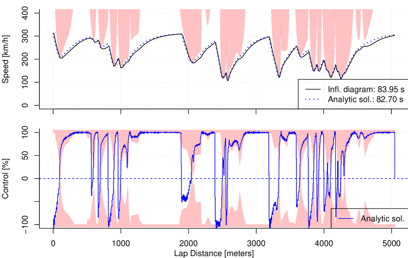
The analytic solution was presented in (Velenis and Tsiotras,, 2008). It is plotted in Figure 7 by a dotted line together with the influence diagram solution. The solutions are quite similar but there are some differences. Apparently, the analytical solution does not fully comply with the acceleration constraints. This causes differences in the speed profiles, otherwise they would be equivalent. We were not able to explain this observation. In the lower part of Figure 7 we present the control profile of the analytic solution reconstructed from the speed profile of the analytic solution.

Figure 7: A comparison of speed profiles: the influence diagram and analytic solution (Velenis and Tsiotras,, 2008). The shaded areas are forbidden by the speed and control constraints, respectively.

6 RELATED WORK

The speed profile optimization problem can be also specified using Markov decision processes (MDPs) (Puterman,, 1994) with a finite horizon, a non-stationary policy and a non-linear stationary reward function. The solution of such an MDP can be found by the approach presented in this paper since solution methods of both approaches are based on dynamic programming. In (Velenis and Tsiotras,, 2008) the problem was solved analytically by methods of the continuous time control (Bertsekas,, 2000) using the Pontryagin’s maximum principle. We compared the influence diagram solution with the analytic solution in Section 5.4 – the solutions were similar. However, analytical solutions for considered extended versions of the problem with an advanced optimization function and additional constraints are not known and numerical methods have to be used.

7 CONCLUSIONS AND FUTURE WORK

We proposed an application of influence diagrams to speed profile optimization and tested it in a real-life scenario. We summarize what we have achieved and what we have learned:

• We were able to find optimal solutions efficiently.

• We verified the solutions are in accordance with the analytical solution of the considered problem.

• An important advantage of influence diagrams is that once the policy is computed, it can be immediately used to update the optimal speed profile under modified circumstances. For example, if the driver has to slow down because of an unexpected traffic situation, the policy immediately provides the best new control value and the speed profile is specified by following the precomputed optimal policies.

• Influence diagrams are especially handy in more complex real-life scenarios where the analytic solution is unknown.

• In applications, different optimality criteria come into play. We can do the computations efficiently as long as they decompose additively along the path segments.

In future we plan to optimize speed profiles using influence diagrams with continuous variables. Inspired by the work of (Kveton et al.,, 2006) on MDPs we plan to study inference in influence diagrams based on mixtures of beta distributions. Other possibilities to be considered are approximations by mixtures of polynomials (Shenoy and West,, 2011; Li and Shenoy,, 2012) or by mixtures of truncated exponentials (Cobb and Shenoy,, 2008; Moral et al.,, 2001).

Currently, we are applying influence diagrams to a more complex scenario with a complex utility function, for which no analytical solution is known. Methods of the control theory, if applied to this scenario, thus need to rely on approximate numerical methods.

Acknowledgements

This work was supported by the Czech Science Foundation through project 13–20012S.

References

- Andersen et al., (1990) Andersen, S. K., Olesen, K. G., Jensen, F. V., and Jensen, F. (1990). HUGIN: a shell for building Bayesian belief universes for expert systems. In Shafer, G. and Pearl, J., editors, Readings in Uncertain Reasoning, pages 332–337. Kaufman.
- Bertsekas, (2000) Bertsekas, D. P. (2000). Dynamic Programming and Optimal Control. Athena Scientific, 2nd edition.
- Chang and Morlok, (2005) Chang, D. J. and Morlok, E. K. (2005). Vehicle speed profiles to minimize work and fuel consumption. Journal of Transportation Engineering, 131(3):173–182.
- Cobb and Shenoy, (2008) Cobb, B. R. and Shenoy, P. P. (2008). Decision making with hybrid influence diagrams using mixtures of truncated exponentials. European Journal of Operational Research, 186(1):261 – 275.
- Cooper, (1988) Cooper, G. (1988). A method for using belief networks as influence diagrams. In Proceedings of the Fourth Conference Annual Conference on Uncertainty in Artificial Intelligence (UAI-88), pages 55–63, Corvallis, Oregon. AUAI Press.
- Cowell et al., (1999) Cowell, R. G., Dawid, A. P., Lauritzen, S. L., and Spiegelhalter, D. J. (1999). Probabilistic Networks and Expert Systems. Springer-Verlag, Berlin-Heidelberg-New York.
- Hellström et al., (2010) Hellström, E., Åslund, J., and Nielsen, L. (2010). Design of an efficient algorithm for fuel-optimal look-ahead control. Control Engineering Practice, 18(11):1318–1327.
- Howard and Matheson, (1981) Howard, R. A. and Matheson, J. E. (1981). Influence diagrams. In Howard, R. A. and Matheson, J. E., editors, Readings on The Principles and Applications of Decision Analysis, volume II, pages 721–762. Strategic Decisions Group.
- Jensen et al., (1994) Jensen, F., Jensen, F. V., and Dittmer, S. L. (1994). From influence diagrams to junction trees. In Proceedings of the Tenth Conference on Uncertainty in Artificial Intelligence, pages 367–373. Morgan Kaufmann.
- Jensen, (2001) Jensen, F. V. (2001). Bayesian Networks and Decision Graphs. Springer-Verlag, New York.
- Jensen and Nielsen, (2007) Jensen, F. V. and Nielsen, T. D. (2007). Bayesian Networks and Decision Graphs, 2nd ed. Springer-Verlag, New York.
- Kveton et al., (2006) Kveton, B., Hauskrecht, M., and Guestrin, C. (2006). Solving factored MDPs with hybrid state and action variables. Journal of Artificial Intelligence Research, 27:153–201.
- Lauritzen and Spiegelhalter, (1988) Lauritzen, S. L. and Spiegelhalter, D. J. (1988). Local computations with probabilities on graphical structures and their application to expert systems (with discussion). Journal of the Royal Statistical Society, Series B, 50:157–224.
- Li and Shenoy, (2012) Li, Y. and Shenoy, P. P. (2012). A framework for solving hybrid influence diagrams containing deterministic conditional distributions. Decision Analysis, 9(1):55–75.
- Mensing et al., (2011) Mensing, F., Trigui, R., and Bideaux, E. (2011). Vehicle trajectory optimization for application in Eco-driving. In Vehicle Power and Propulsion Conference (VPPC), IEEE, pages 1–6.
- Monastyrsky and Golownykh, (1993) Monastyrsky, V. V. and Golownykh, I. M. (1993). Rapid computation of optimal control for vehicles. Transportation Research Part B: Methodological, 27(3):219 – 227.
- Moral et al., (2001) Moral, S., Rumi, R., and Salmerón, A. (2001). Mixtures of truncated exponentials in hybrid bayesian networks. In Benferhat, S. and Besnard, P., editors, Symbolic and Quantitative Approaches to Reasoning with Uncertainty, volume 2143 of Lecture Notes in Computer Science, pages 156–167. Springer Berlin Heidelberg.
- Oxford Technical Solutions, (2002) Oxford Technical Solutions (2002). RT3000 inertial and GPS measurement system. Technical report, Oxfordshire, UK.
- Puterman, (1994) Puterman, M. L. (1994). Markov Decision Processes: Discrete Stochastic Dynamic Programming. John Wiley & Sons, New York, NY.
- R Core Team, (2014) R Core Team (2014). R: A Language and Environment for Statistical Computing. R Foundation for Statistical Computing, Vienna, Austria.
- Rakha et al., (2012) Rakha, H. A., Kamalanathsharma, R. K., and Ahn, K. (2012). Aeris: Eco-vehicle speed control at signalized intersections using i2v communication. Technical Report FHWA-JPO-12-063, Virginia Polytechnic Institute and State University and Virginia Tech Transportation Institute.
- Saboohi and Farzaneh, (2009) Saboohi, Y. and Farzaneh, H. (2009). Model for developing an eco-driving strategy of a passenger vehicle based on the least fuel consumption. Applied Energy, 86(10):1925–1932.
- Shachter, (1986) Shachter, R. D. (1986). Evaluating influence diagrams. Operations Research, 34(6):871–882.
- Shachter and Peot, (1992) Shachter, R. D. and Peot, M. A. (1992). Decision making using probabilistic inference methods. In Proceedings of the Eighth Conference Annual Conference on Uncertainty in Artificial Intelligence (UAI-92), pages 276–283, San Mateo, CA. Morgan Kaufmann.
- Shenoy, (1992) Shenoy, P. P. (1992). Valuation based systems for bayesian decision analysis. Operations Research, 40:463–484.
- Shenoy and West, (2011) Shenoy, P. P. and West, J. C. (2011). Inference in hybrid bayesian networks using mixtures of polynomials. International Journal of Approximate Reasoning, 52(5):641–657.
- Velenis and Tsiotras, (2008) Velenis, E. and Tsiotras, P. (2008). Minimum-time travel for a vehicle with acceleration limits: Theoretical analysis and receding-horizon implementation. Journal of Optimization Theory and Applications, 138(2):275–296.