Quark-hadron phase transition in massive gravity

Abstract

We study the quark -hadron phase transition in the framework of massive gravity. We show that the modification of the FRW cosmological equations leads to the quark -hadron phase transition in the early massive Universe. Using numerical analysis, we consider that a phase transition based on the chiral symmetry breaking after the electroweak transition, occurred at approximately $10\mu$ seconds after the Big Bang to convert a plasma of free quarks and gluons into hadrons.

1 Introduction

In the expanding and cooling standard cosmology, the early Universe experiences a series of symmetry-breaking phase transitions, resulted of the topological defects forming. Study such phase transitions help us to understand better the evolution of the early Universe, characterized by the existence of a quark-gluon plasma phase transition. In this way, we concentrate on possible scenarios which allow such a phase transition occurrence. Here, we follow [1] which have considered the quark-gluon phase transition in a cosmologically transparent perspective. It is worth mentioning that QCD predicts the existence of phase transition from the quark-gluon plasma phase to hadron gas one. The phase transition in QCD which depends on singular behavior of the partition function, can be described by a first or second order phase transition, and also it can be outlined by a crossover phase transition, that depends on the values of the quark masses. First time, the possibility of a phase transition in the gas of quark-gluon bags was studied in [2]. The results of the first, second and higher order transitions have been presented in literatures. Furthermore, the possibility of no phase transitions was mentioned in [3]. Lattice QCD calculations carried out for two quark flavors propound that QCD makes a smooth crossover transition at a temperature of $T_{c}\sim 150$ MeV [4]. In the early Universe crossover phase transition may be responsible for the formation of relic quark -gluon objects which may have survived. In this work, we study the phase transition under certain conditions that a gas of extended hadrons could generate phase transitions of the first or second order, and also we consider a smooth crossover transition which is qualitatively same as the lattice QCD.

The color deconfined quark–gluon plasma cooling down, below the critical temperature believed to be around $T_{c}\sim 150$ MeV leads to form color confined hadrons (mainly pions and a tiny amount of neutrons and protons, since the net baryon number should be conserved). Therefore, such a new phase does not assemble quickly. Actually, a first order phase transition requires some supercooling to produce the energy used in composing the surface of the bubble and the new hadron phase. In [5] a first order quark-hadron phase transition in the expanding Universe has been expressed. During the hadron bubble nucleating, hidden heat is blurted and a spherical shock wave propagates to the surrounding supercooled quark gluon plasma. The plasma thus formed is reheated and reaches the critical temperature, preventing further nucleation in a region shifted by means of one or more shock fronts. Generally, bubble growth is explained by deflagrations where a shock front precedes the actual transition front. The ending of the nucleation occurs when the whole Universe has reheated $T_{c}$. The prompt stopping of this phase transition, in about $0.05\mu$s, contributes the cosmic expansion completely insignificant over this period. Finally, the transition ends when all quark-gluon plasma has been reformed into hadrons surrender of possible quark nugget production. The quark-hadron phase transition and its cosmological implications have been widely studied in the context of general relativistic cosmology in [6]-[21].

In this paper we study quark-gluon phase transition in the framework of a covariant massive gravity model recently proposed in [22, 23]. In order to have a consistent theory, nonlinear terms should be tuned to remove order by order the negative energy state in the spectrum [24]. The model under consideration follows from a scheme originally studied in [25, 26] and at the complete nonlinear level with an arbitrary reference metric has been not found any ghosts [27, 28]. The treated theory exploits several important features. Actually, the graviton mass typically demonstrates itself on cosmological scales at late times thus providing a natural explanation of the late lime acceleration of the Universe [29]. Additionally, the theory has exotic solutions in which the graviton mass affects the dynamics at early times. We show that in the massive gravity theory, it is possible to have cosmological quark-gluon phase transition and it exists even for spatially flat (i.e. ${\cal K}=0$) cosmological models.

2 Massive cosmological equations

We review cosmological equations of the massive gravity introduced in [22, 23]. According to the formalism used in [30], we define a four-dimensional pseudo-Riemannian manifold $({\cal M},g)$ and the dynamics can be determined by the action as follows

$$S=-\frac{1}{8\pi G}\int\left(\frac{1}{2}R+m^{2}\mathcal{U}\right)d^{4}x\ +\ S_{m},$$

where $G$, $R$ and $S_{m}$ are the Newton gravitational constant, the Ricci scalar and ordinary matter field action, respectively. The mass coupled potential term is defined by

$$\mathcal{U} = \frac{1}{2}(K^{2}-K^{\nu}_{\mu}K^{\mu}_{\nu})+\frac{c_{3}}{3!}\epsilon_{\mu\nu\rho\sigma}\epsilon^{\alpha\beta\gamma\sigma}K_{\alpha}^{\mu}K_{\beta}^{\nu}K_{\gamma}^{\rho}$$

$$+\frac{c_{4}}{4!}\epsilon_{\mu\nu\rho\sigma}\epsilon^{\alpha\beta\gamma\delta}K_{\alpha}^{\mu}K_{\beta}^{\nu}K_{\gamma}^{\rho}K_{\delta}^{\sigma},$$

here $c_{3}$, $c_{4}$ are arbitrary dimensionless real constants and also $\epsilon_{\mu\nu\rho\sigma}$ is the Levi-Civita tensor density.

$$K^{\mu}_{\nu}=\delta^{\mu}_{\nu}-\gamma^{\mu}_{\nu},$$

$\gamma^{\mu}_{\nu}$ being defined by the relation

$$\gamma^{\mu}_{\sigma}\gamma^{\sigma}_{\nu}=g^{\mu\sigma}f_{\sigma\nu},$$

with $f_{\sigma_{\nu}}$ that is, a symmetric tensor field. The quantity $m_{g}=\hbar m/c$ is called the graviton mass.

We consider the Friedmann-Lemaître-Robertson-Walker (FLRW) Universe with three-dimensional spatial curvature ${\cal K}=0,\pm 1$, explained by the line element

$$ds^{2} = g_{\mu\nu}dx^{\mu}dx^{\nu}$$

$$= dt^{2}-a(t)^{2}\left[\frac{dr^{2}}{1-{\cal K}r^{2}}+r^{2}(d\theta^{2}+\sin(\theta)^{2}d\phi^{2})\right].$$

The first Friedmann equation for generic values of the dimensionless constants $c_{3}$ and $c_{4}$ and imposing the Bianchi identities, reads

$$3\frac{\dot{a}^{2}+{\cal K}{a^{2}}}{a^{2}} = m^{2}\left(4c_{3}+c_{4}-6+3C\frac{3-3c_{3}-c_{4}}{a}\right.$$ (2)

$$\left.+3C^{2}\frac{c_{4}+2c_{3}-1}{a^{2}}-C^{3}\frac{c_{3}+c_{4}}{a^{3}}\right)+8\pi G\rho~{},$$

where $C$ is an integration constant. The conservation equations for the matter component is

$$\dot{\rho}+3H(\rho+p)=0~{},$$ (3)

with $H=\dot{a}/a$. Also we define a constant equation of state parameter $w=p/\rho$.
Furthermore, in the consequent analysis the parameter space is reduced to the subset $c_{3}=-c_{4}$ [31], that is the simplest choice that presents a successful Vainshtein effect in the weak field limit.

We can rewrite equation (2) as follows

$$H^{2}=\frac{\kappa}{3}\rho-\frac{\mathcal{K}}{a^{2}}+\frac{m^{2}}{3}\left(A_{1}+\frac{A_{2}}{a}+\frac{A_{3}}{a^{2}}\right),$$ (4)

where $\kappa=8\pi G$, $a/C\rightarrow a$ and

$$A_{1}=-3c_{4}-6,~{}~{}~{}~{}~{}~{}~{}~{}~{}~{}A_{2}=3\left(3+2c_{4}\right),~{}~{}~{}~{}~{}~{}~{}~{}~{}A_{3} = -3\left(1+c_{4}\right).$$ (5)

3 Quark–hadron phase transition

In this section, we interpret the appropriate physical quantities of the quark–hadron phase transition, which will be used in the following sections in the framework of the massive gravity. We know that at the phase transition the scale of the cosmological QCD transition is given by the Hubble radius $H^{-1}$, which is $H^{-1}\sim M_{4}/T^{2}_{c}\sim 10$ km, here $T_{c}$ is the critical temperature. Inside of the Hubble volume has the mass about $\sim 1M_{\odot}$. The timescale of QCD is $1$ fm/c $\approx 10^{-23}$ s which should be compared with the expansion time scale, $10^{-5}$ s. Even the rate of the weak interactions passes the Hubble rate by a factor of $10^{7}$. As a result, in this phase photons, leptons, quarks and gluons (or pions) are lightly coupled and may be characterized as a single, adiabatically expanding fluid [12]. In consideration of the quark–hadron phase transition it is essential to determine the equation of state of the matter, in both hadron and quark state. Specifying an equation of state is equivalent to give the chemical potential $\mu$ and the pressure as a function of the temperature $T$. The quark chemical potentials at high temperatures are equal, because weak interactions keep them in chemical equilibrium, and the chemical potentials for leptons are zero. So the chemical potential for a baryon is characterized by $\mu_{B}=3\mu_{q}$ . The baryon number density of an ideal Fermi gas of three quark flavors is defined by $n_{B}\approx T^{2}\mu_{B}/3$ which leads to $\mu_{B}/T\sim 10^{-9}$ at $T>T_{c}$. At low temperatures $\mu_{B}/T\sim 10^{-2}$. Thus, an excellent approximation for the study of the equation of state of the cosmological matter in the early Universe, is assumption of a vanishing chemical potential at the phase transition temperature in both quark and hadron phase. In addition to the strongly interacting matter, we suppose that in each phase there are present leptons and relativistic photons, obeying equations of state similar to that of hadronic matter [6]. The equation of state of the matter in the quark phase can be have the following form

$$\rho_{q}=3a_{q}T^{4}+V(T),~{}~{}~{}~{}~{}~{}~{}~{}~{}~{}~{}~{}p_{q}=a_{q}T^{4}-V(T),$$ (6)

where $a_{q}=(\pi^{2}/90)g_{q}$, with $g_{q}=16+(21/2)N_{F}+14.25=51.25$ and $N_{F}=2$. $V(T)$ is the self-interaction potential. For $V(T)$ we use the expression in [19]

$$V(T)=B+\gamma_{T}T^{2}-\alpha_{T}T^{4},$$ (7)

where $B$ is the bag pressure constant, $\alpha_{T}=7\pi^{2}/20$ and $\gamma_{T}=m^{2}_{s}/4$ with $m_{s}$ the mass of the strange quark in the range $m_{s}\in(60-200)$ MeV. The potential form $V$ corresponds to a physical model in which the quark fields are interacting with a chiral field constructed with a scalar field and the $\pi$ meson field. By ignoring the temperature effects, the equation of state in the quark phase is in the form of $p_{q}=(\rho_{q}-4B)/3$, in the MIT bag model. Results gained in low energy hadron spectroscopy, heavy ion collisions and phenomenological fits of light hadron properties give $B^{1/4}$ between $100$ and $200$ MeV [25]. In the hadron phase, we take the cosmological fluid which consists of an ideal gas of massless pions and of nucleons explained by the Maxwell -Boltzmann statistics, with energy density $\rho_{h}$ and pressure $p_{h}$, respectively. The equation of state can be written approximately as

$$p_{h}(T)=\frac{1}{3}\rho_{h}(T)=a_{\pi}T^{4},$$ (8)

where $a_{\pi}=(\pi^{2}/90)g_{h}$ and $g_{h}=17.25$.

The critical temperature $T_{c}$ is defined by the condition $p_{q}(T_{c})=p_{h}(T_{c})$ [6], and in the present model given by

$$T_{c}=\left(\frac{\gamma_{T}+\sqrt{\gamma_{T}^{2}+4B(a_{q}+\alpha_{T}-a_{\pi})}}{2(a_{q}+\alpha_{T}-a_{\pi})}\right)^{1/2}.$$ (9)

For $m_{s}=200$ MeV and $B^{1/4}=200$ MeV the transition temperature is of the order $T_{c}\approx 125$ MeV. When the phase transition is of first order, all the physical quantities, like the energy density, pressure and entropy have discontinuities behavior across the critical curve. The ratio of the quark and hadron energy densities at the critical temperature, $\rho_{q}(T_{c})/\rho_{h}(T_{c})$, is of the order of $3.62$ for $m_{s}=200$ MeV and $B^{1/4}=200$ MeV. If the temperature effects in the self-interaction potential $V$ are neglected, $\alpha_{T}=\gamma_{T}\approx 0$, thus we get the well-known relation between the bag constant and critical temperature, $B=(g_{q}-g_{h})\pi^{2}T^{4}_{c}/90$ [6].

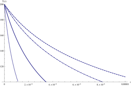
Figure 1: Variation of $T(\tau)$ as a function of time ($\tau$) for different values of $c_{4}$: $c_{4}=8\times 10^{8}$ (solid curve), $c_{4}=8\times 10^{9}$ (dashed curve), $c_{4}=2\times 10^{10}$ (dotted curve) and $c_{4}=1\times 10^{11}$ (dotted-dashed curve). We have taken $B^{1/4}=200$ MeV, $\kappa=1$ and ${\cal K}=-1$.

4 Dynamical interpretation of the massive Universe during the quark–hadron phase transition

The quantities to be followed through the quark-hadron phase transition in the massive gravity are the temperature $T$, the energy density $\rho$ and the scale factor $a$. Note that these quantities are determined by the gravitational field equations (4) and (3) and by the equations of state (6), (7) and (8). We must study now the evolution of the massive Universe before, during and after the phase transition.

Before the phase transition, $T>T_{c}$ the massive Universe is in the quark phase. With the use of the equations of state of the quark matter, and the conservation equations for the matter component, equation (3) can be written in the form

$$H=\frac{\dot{a}}{a}=-\frac{3a_{q}-\alpha_{{}_{T}}}{3a_{q}}\frac{\dot{T}}{T}-\frac{1}{6}\frac{\gamma_{{}_{T}}}{a_{q}}\frac{\dot{T}}{T^{3}},$$ (10)

by integrating we have scale factor-temperature relation as

$$a(T)=a_{0}~{}T^{\frac{\alpha_{{}_{T}}-3a_{q}}{3a_{q}}}\exp\left(\frac{1}{12}\frac{\gamma_{{}_{T}}}{a_{q}}\frac{1}{T^{2}}\right),$$ (11)

where $a_{0}$ is a constant of integration.

By using equation (10) we have an expression, describing the evolution of the temperature of the massive Universe in the quark phase, given by

$$\frac{dT}{d\tau} = \frac{-T^{3}}{U_{0}T^{2}+U_{1}}\times$$

$$\sqrt{\frac{1}{3}m^{2}\left(\frac{A_{3}T^{-2\xi}e^{-\frac{\eta}{T^{2}}}}{a_{0}^{2}}+\frac{A_{2}T^{-\xi}e^{-\frac{\eta}{2T^{2}}}}{a_{0}}+A_{1}\right)+\frac{1}{3}\kappa\left(3a_{q}T^{4}+B-\alpha_{T}T^{4}+\gamma_{T}T^{2}\right)-\frac{{\cal K}T^{-\xi}e^{-\frac{\eta}{T^{2}}}}{a_{0}^{2}}},$$

where we have denoted

$$U_{0}=1-\frac{\alpha_{{}_{T}}}{3a_{{}_{T}}},~{}~{}~{}~{}~{}~{}~{}\eta=\frac{\gamma_{T}}{6a_{q}},~{}~{}~{}~{}~{}~{}~{}~{}\xi=\frac{\alpha_{T}-3a_{q}}{3a_{q}},~{}~{}~{}~{}~{}U_{1}=\frac{\gamma_{{}_{T}}}{6a_{q}}.$$ (13)

We solve equation (4) numerically and the result is presented in Figure 1 which shows the behavior of temperature as a function of cosmic time $\tau$ in a massive Universe filled with quark matter for different values of $c_{4}$. It can be seen that the temperature drops faster for higher values of $c_{4}$.

4.1 Self-interaction potential $(V(T)=B)$

Let us take attention on the phase transition era, namely the simple case where temperature corrections can be neglected in the self-interaction potential $V$. Then $V=B={\rm cons.}$ and equation of state of the quark matter is given by that of the bag model, $p_{q}=\left(\rho_{q}-4B\right)/3$. Equation (3) may then be integrated to give the scale factor massive Universe as a function of temperature

$$a(T)=\frac{c}{T},$$ (14)

where $c$ is a constant of integration.

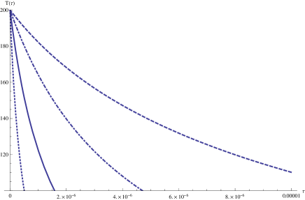
Figure 2: Variation of $T(\tau)$ as a function of time ($\tau$) for different values of $c_{4}$: $c_{4}=8\times 10^{8}$ (solid curve), $c_{4}=8\times 10^{9}$ (dashed curve), $c_{4}=2\times 10^{10}$ (dotted curve) and $c_{4}=1\times 10^{11}$ (dotted-dashed curve). We have taken $B^{1/4}=200$ MeV, $\kappa=1$ and ${\cal K}=-1$.

Using equations (3) and (4), the time dependence of temperature can be written as follows

$$\frac{1}{T}\frac{dT}{d\tau}=-\sqrt{\frac{\kappa}{3}\left(3a_{q}T^{4}+B\right)-{\cal K}T^{{}^{2}}+\frac{m^{2}}{3}\left(A_{1}+A_{2}T+A_{3}T^{{}^{2}}\right)}.$$ (15)

The equation (15) can be solved numerically and plotted in figure 2 which shows the behavior of temperature as a function of cosmic time $\tau$ in a massive Universe filled with quark matter for different values of $c_{4}$.

4.2 Formation of hadrons

In the phase transition regime, pressure and temperature are constant and quantities like the entropy $S=sa^{3}$ and enthalpy $W=\left(\rho+p\right)a^{3}$ are conserved. Following [1, 6], we substitute $\rho\left(\tau\right)$ by $h(\tau)$, the volume fraction of matter in the hadron phase, by defining

$$\rho\left(\tau\right)=\rho_{{}_{H}}h(\tau)+\rho_{{}_{Q}}\left[1-h(\tau)\right]=\rho_{{}_{Q}}\left[1+nh(\tau)\right],$$ (16)

where $n=\left(\rho_{{}_{H}}-\rho_{{}_{Q}}\right)/\rho_{{}_{Q}}$. Start of the phase transition is described by $h(\tau_{c})=0$ where $\tau_{c}$ is the time representing the beginning of the phase transition and $\rho\left(\tau_{c}\right)\equiv\rho_{{}_{Q}}$, during the end of the transition is characterized by $h\left(\tau_{h}\right)=1$ with $\tau_{h}$ being the time signalling the end and corresponding to $\rho\left(\tau_{h}\right)\equiv\rho_{{}_{H}}$. For $\tau>\tau_{h}$ the Universe goes to the hadronic phase.

Now, equation (3) gives

$$\frac{\dot{a}}{a}=-\frac{1}{3}\frac{\left(\rho_{{}_{H}}-\rho_{{}_{Q}}\right)\dot{h}}{\rho_{{}_{Q}}+p_{c}+\left(\rho_{{}_{H}}-\rho_{{}_{Q}}\right)h}=-\frac{1}{3}\frac{r\dot{h}}{1+rh},$$ (17)

where we have implied $r=\left(\rho_{{}_{H}}-\rho_{{}_{Q}}\right)/\left(\rho_{{}_{Q}}+p_{c}\right)$. From the above equation we can obtain the relation between the scale factor and the hadron fraction $h(\tau)$

$$a(\tau)=a\left(\tau_{c}\right)\left[1+rh(\tau)\right]^{-1/3},$$ (18)

where the initial condition $h\left(\tau_{c}\right)=0$ has been used. Now, using equations (4) and (18) we get the time evolution of the matter fraction in the hadronic phase

$$\frac{dh}{d\tau} = -3\left(h+\frac{1}{r}\right)\times$$

$$\sqrt{\frac{\kappa\rho_{{}_{Q}}\left[1+nh(\tau)\right]}{3}-\frac{{\cal K}\left[1+rh(\tau)\right]}{a^{2}\left(\tau_{c}\right)}^{2/3}+\frac{m^{2}}{3}\left(A_{1}+\frac{A_{2}\left[1+rh(\tau)\right]^{1/3}}{a\left(\tau_{c}\right)}+\frac{A_{3}\left[1+rh(\tau)\right]^{2/3}}{a^{2}\left(\tau_{c}\right)}\right)}.$$

Figure 2 shows variation of the hadron fraction $h(\tau)$ as a function of $\tau$ for different values of $c_{4}$. The higher values of $c_{4}$ end the phase transition in shorter period of time.

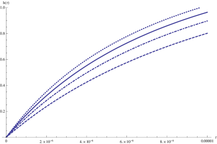
Figure 3: Variation of $h(\tau)$ as a function of time ($\tau$) for different values of $c_{4}$: $c_{4}=8\times 10^{8}$ (solid curve), $c_{4}=8\times 10^{9}$ (dashed curve), $c_{4}=2\times 10^{10}$ (dotted curve) and $c_{4}=1\times 10^{11}$ (dotted-dashed curve). We have taken $B^{1/4}=200$ MeV, $\kappa=1$ and ${\cal K}=-1$.

4.3 Pure hadronic era

The scale factor of the Universe at the end of the phase transition has the value

$$a\left(\tau_{h}\right)=a\left(\tau_{c}\right)\left(r+1\right)^{\frac{-1}{3}}.$$ (20)

Also, the energy density of the pure hadronic matter after the phase transition is $\rho_{h}=3p_{h}=3a_{\pi}T^{4}$. The conservation equation (3) gives $a(T)=a\left(\tau_{h}\right)T_{c}/T$. The temperature dependence of the massive Universe in the hadronic phase is governed by the equation

$$\frac{dT}{d\tau}=-T\sqrt{\kappa a_{\pi}T^{4}-\frac{{\cal K}}{a^{2}\left(\tau_{h}\right)T_{c}^{2}}T^{2}+\frac{m^{2}}{3}\left(A_{1}+\frac{A_{2}}{a\left(\tau_{h}\right)T_{c}}T+\frac{A_{3}}{a^{2}\left(\tau_{h}\right)T_{c}^{2}}T^{2}\right)}.$$ (21)

Variation of temperature of the hadronic fluid filled massive Universe as a function of $\tau$ for different values of $c_{4}$ is depicted in figure 3. The hadronic fluid cools down faster for higher values of $c_{4}$.

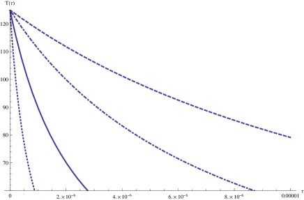
Figure 4: Variation of $T(\tau)$ as a function of time ($\tau$) for different values of $c_{4}$: $c_{4}=8\times 10^{8}$ (solid curve), $c_{4}=8\times 10^{9}$ (dashed curve), $c_{4}=2\times 10^{10}$ (dotted curve) and $c_{4}=1\times 10^{11}$ (dotted-dashed curve). We have taken $B^{1/4}=200$ MeV, $\kappa=1$ and ${\cal K}=-1$.

5 Hight and low temperature equation of state in lattice QCD

QCD phase transition is an important character of the particle physics in which it is more relevant to any studied mechanisms responsible for the evolution of the early Universe. In such a scenario, under a crossover transition a soup of quarks and gluons interact and undergo to form hadrons. To study the Universe at early times within the context of massive gravity in the lattice QCD, we must have a short review of the basic conceptions before using the results achieved in such a phase transition. Lattice QCD is a new access that allows one to systematically consider the non-perturbative regime of the QCD equation of state. The QCD equation of state was calculated by supercomputers on the lattice in [39] with a heavier strange quark and two light quarks on a $(N_{t}=6)32^{3}$ size lattice. See [39, 42] for recent results in lattice QCD at high temperature. We see that during the high temperature regime, radiation like behavior in the region at and below the critical temperature $T_{c}(\approx 200$ MeV) of the de-confinement transition changes remarkably. We will see in the next section this change in behavior will also be relevant for cosmological observables. For high temperatures interval $2.82(100$ MeV) and $7.19(100$ MeV) data fitting give a simple form of equation of state as

$$\rho_{{}_{High}}(T)\approx\alpha T^{4},$$ (22)

$$p_{{}_{High}}(T)\approx\sigma T^{4}.$$

By using a least squares fit, one can get $\alpha=14.9702\pm 009997$ and $\sigma=4.99115\pm 004474$ [39]. While for times before the phase transition the lattice data match the radiation behavior very well, for times corresponding to temperatures above $T_{c}$ the behavior of the lattice data changes towards that of the matter dominated phase. We notice that lattice studies on QCD show that the phase transition is actually a crossover transition.

In addition to, there is an other approach to the low temperature equation of state in the lattice QCD named Hadronic Resonance Gas model (HRG)in which QCD in the confinement phase is considered as an non-interacting gas of fermions and bosons [43]. The conception of the HRG model is to basically account for the strong interaction in the confinement phase by looking at the hadronic resonances only, since these are implicity the relevant degrees of freedom in that phase. The HRG model predicts a good description of thermodynamic quantities in the transition region from high to low temperatures [44]. The trace anomaly result in HRG can also be parameterized as [45]

$$\frac{\Theta(T)}{T^{4}}\equiv\frac{\rho-3p}{T^{4}}=a_{1}T+a_{2}T^{3}+a_{3}T^{4}+a_{4}T^{10},$$ (23)

with $a_{1}=4.654GeV^{-1}$, $a_{2}=-879GeV^{-3},$ $a_{3}=8081GeV^{-4}$ and $a_{4}=-7039000GeV^{-10}$.

The calculation of the pressure, entropy density and energy density in lattice QCD, usually arises from the calculation of the trace anomaly $\Theta(T)=\rho(T)-3p(T)$. Using the conventional thermodynamic identity, the pressure difference at temperatures $T$ and $T_{low}$ can be written as the integral of the trace anomaly

$$\frac{p(T)}{T_{4}}-\frac{p(T_{low})}{T^{4}_{low}}=\int^{T}_{T_{low}}\frac{dT^{\prime}}{T^{5}\Theta(T^{\prime})}.$$ (24)

By taking the lower integration limit adequately small, $p(T_{{}_{low}})$ can be neglected due to the exponential suppression and the energy density $\rho(T)=\Theta(T)+3p(T)$ and entropy density $s(T)=(\rho+p)/T$ can be calculated. This technique is known as the integral method [46]. Using equations (23) and (24), we get

$$\rho_{{}_{Low}}(T)=\eta T^{4}+4a_{1}T^{5}+2a_{2}T^{7}+\frac{7a_{3}}{4}T^{8}+\frac{13a_{4}}{10}T^{14},$$ (25)

where $\eta=-0.112$. The trace anomaly plays an essential role in lattice determination of the equation of state. The equation of state is obtained by integrating the parameterizations given in (23) over temperature as shown in (24).

6 Massive Universe and QCD phase transition

6.1 High temperature regime

To continue, let us consider the era before the phase transition at high temperature where the Universe is in the quark phase. Using the conservation equation of matter and equation of state of quark matter (22), one can write the Hubble parameter relation as

$$H=\frac{\dot{a}}{a}=-\frac{4\alpha}{3(\alpha+\sigma)}\frac{\dot{T}}{T},$$ (26)

thus, one can solve for the scale factor

$$a(T)=w_{3}T^{\frac{-4\alpha}{3(\alpha+\sigma)}},$$ (27)

where $w_{3}$ is an integration constant.

We can write an expression to describe the behavior of temperature of the massive Universe as a function of time the quark phase. Using (22) and (4), we get a differential equation for the temperature as follows

$$\frac{dT}{dt}=-\frac{3(\alpha+\sigma)T}{4\alpha}\sqrt{\frac{\kappa}{3}\rho(T)-\frac{\mathcal{K}}{a(T)^{2}}+\frac{m^{2}}{3}\left(A_{1}+\frac{A_{2}}{a(T)}+\frac{A_{3}}{a(T)^{2}}\right)},$$ (28)

here we have set $w_{3}=1$. In compatible with the HRG equation of state the lower temperature limit is $T<170$MeV. Equation (28) may be solved numerically and the result is depicted in Fig. 4, which presents the behavior of temperature of the Universe in the quark phase as a function of cosmic time in massive cosmology for different values of the $c_{4}$, in the interval $282$ MeV$<T<719$MeV in high temperature regime. It can be seen that as the time grows the Universe becomes cooler.

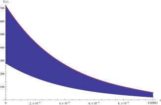
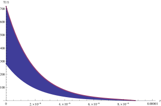
Figure 5: The behavior of $T(\tau)$ in interval $282$ MeV $<T<719$ MeV as a function of $\tau$ for values of $c_{4}=6\times 10^{10}$ (left) and $c_{4}=3\times 10^{11}$ (right). We have taken $\kappa=1$ and ${\cal K}=-1$.

6.2 Low temperature regime

In this subsection we study the era before phase transition at low temperature where the Universe is in the confinement phase and is expressed as a non-interacting gas of fermions and bosons [43]. Using the equation of state (25) together with conservation equation of matter, we obtain the Hubble parameter as

$$H=\frac{\dot{a}}{a}=-\frac{12\eta T^{3}+20a_{1}T^{4}+A(T)}{3[4\eta T^{4}+5a_{1}T^{5}+B(T)]}\dot{T},$$ (29)

where

$$A(T)=14a_{2}T^{6}+14a_{3}T^{7}+\frac{91}{5}T^{13},$$ (30)

$$B(T)=73a_{2}T^{7}+2a_{3}T^{8}+75a_{4}T^{14}.$$

We may now solve for the scale factor and obtain

$$a(T)=\frac{w_{4}}{T(75a_{1}T+35a_{2}T^{3}+30a_{3}T^{4}+21T^{10}+60\eta)^{1/3}},$$ (31)

where $w_{4}$ is an integration constant. We can write an expression to explain the behavior of temperature of the massive Universe as a function of time in the quark phase. By using (25) and (4), one can write a differential equation for temperature as follows

$$\frac{dT}{dt}=-\frac{3[4\eta T^{4}+5a_{1}T^{5}+B(T)]T}{12\eta T^{3}+20a_{1}T^{4}+A(T)}\sqrt{\frac{\kappa}{3}\rho(T)-\frac{\mathcal{K}}{a(T)^{2}}+\frac{m^{2}}{3}\left(A_{1}+\frac{A_{2}}{a(T)}+\frac{A_{3}}{a(T)^{2}}\right)}$$ (32)

where we have set $w_{4}=1$. We have solved equation (32) numerically, and the result is depicted in Fig. 5, which presents the behavior of temperature of the Universe in the quark phase as a function of the cosmic time for different values of $c_{4}$, in the interval $80$ MeV $<T<180$ MeV at the low temperature regime. From Fig. 5 it can be seen that in the context of the HRG model, $c_{4}$ enhances the cooling process. It seems in our model the phase transition depends on $c_{4}$ and can be interpreted as a running coupling constant for the phase transition.

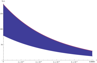
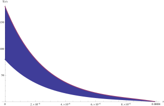
Figure 6: The behavior of $T(\tau)$ in interval $282$ MeV $<T<719$ MeV as a function of $\tau$ for values of $c_{4}=6\times 10^{10}$ (left) and $c_{4}=3\times 10^{11}$ (right). We have taken $\kappa=1$ and ${\cal K}=-1$.

7 Conclusion

In this paper, we have considered the quark -hadron phase transition in the massive gravity, within an effective model of QCD. We have studied the time evolution of the physical quantities in the early Universe, such as; the energy density, temperature and scale factor, before, during, and after the phase transition. Also, in the context of crossover transition for high and low temperatures we have discussed the time evolution of temperature and scale factor of the early Universe which is presented in section five.

We have shown that the effective temperature of the quark gluon plasma and of the hadronic fluid for different values of $c_{4}$ phase transition occurs and it decreases. Comparing Figs. 4 and 5, it can be seen that for the above mentioned two models the slope of temperature, $T$ , is different during the crossover transition. Taking into account the energy range in which the calculations are done, one might conclude that these two approaches to the quark -hadron transition in the early Universe do not predict fundamentally different ways of the evolution of the early Universe. Note that in the massive gravity theory it is possible to have cosmological quark-gluon phase transition and it exists even for spatially flat and closed (i.e. ${\cal K}=0,+1$) cosmological models.

References

- [1] G. De Risi, T. Harko, F. S. N. Lobo and C. S. J. Pun, Nucl. Phys. B 805 (2008) 190, gr-qc/ 0807.3066.
-
[2]
M. I. Gorenstein, V. K. Petrov and G. M. Zinovjev, Phys. Lett. B 106 (1981) 327;
M. I. Gorenstein , V. K. Petrov, V. P. Shelest and G. M. Zinovev, Theor. Math. Phys. 52 (1982) 843. -
[3]
M. I. Gorenstein, W. Greiner and Yang Shin Nan, J. Phys. G: Nucl. Part. Phys. 24 (1998) 725;
M. I. Gorenstein, M. Gazdzicki and W. Greiner, Phys. Rev. C 72 (1998) w024909;
I. Zakout, C. Greiner and J. Schaffner-Bielich, Nucl. Phys. A 781 (2007) 150;
I. Zakout and C. Greiner, Phys. Rev. C 78 (2008) 034916;
K. A. Bugaev, Phys. Rev. C 76 (2007) 014903;
K. A. Bugaev, V. K. Petrov and G. M. Zinovjev, arXiv: 0904.4420;
A. Bessa, E. S. Fraga and B. W. Mintz, Phys. Rev. D 79 (2009) 034012. -
[4]
Y. Aoki, Sz. Borsanyi, S. Durr, Z. Fodor, S. D. Katz, S. Krieg and K. K. Szabo, JHEP 0906
(2009) 088, arXiv: 0903.4155 ;
A. Bazavov, et al, Phys. Rev. D 80 (2009) 014504, arXiv: 0903.4379;
L. Ferroni and V. Koch, Phys. Rev. C 79 (2009) 034905;
C. De Tar, PoS LATTICE 2008 (2008) 001, arXiv: 0811.2429;
Y. Aoki, G. Endrodi, Z. Fodor, S. D. Katz and K. K. Szabo, Nature 443 (2006) 675;
P. de Forcrand and O. Philipsen, JHEP 070 (2007) 077, hep-lat/0607017;
Z. G. Tan and A. Bonasera, Nucl. Phys. A 784, 368 (2007). - [5] K. Kajantie, H. Kurki-Suonio, Phys. Rev. D 34 (1986) 1719.
- [6] J. Ignatius, K. Kajantie, H. Kurki-Suonio and M. Laine, Phys. Rev.D 49(1994) 3854.
- [7] J. Ignatius, K. Kajantie, H. Kurki-Suonio and M. Laine, Phys. Rev. D 50 (1994) 3738.
- [8] H. Kurki-Suonio and M. Laine, Phys. Rev. D 51, 5431 (1995).
- [9] H. Kurki-Suonio and M. Laine, Phys. Rev. D 54(1996) 7163.
- [10] M. B. Christiansen and J. Madsen, Phys. Rev. D 53 (1996) 5446.
- [11] L. Rezzolla, J. C. Miller and O. Pantano, Phys. Rev. D 52 (1995) 3202.
- [12] L. Rezzolla and J. C. Miller, Phys. Rev. D 53(1996) 5411.
- [13] L. Rezzolla, Phys. Rev. D 54 (1996) 1345.
- [14] L. Rezzolla, Phys. Rev. D 54 (1996) 6072.
- [15] A. Bhattacharyya, J. -e. Alam, S. S. P. Roy, B. Sinha, S. Raha and P. Bhattacharjee, Phys. Rev. D 61 (2000) 083509.
- [16] A. C. Davis and M. Lilley, Phys. Rev. D 61 (2000) 043502.
- [17] N. Borghini, W. N. Cottingham and R. Vinh Mau, J. Phys. G 26 (2000) 771.
- [18] H. I. Kim, B.-H. Lee and C. H. Lee, Phys. Rev. D 64 (2001) 067301.
- [19] J. Ignatius and D. J. Schwarz, Phys. Rev. Lett. 86 (2001) 2216.
- [20] M. Heydari-Fard and H. R. Sepangi, Class. Quantum Grav. 26 (2009) 235021.
-
[21]
K. Atazadeh, A. M. Ghezelbash and H. R. Sepangi, Class. Quantum
Grav. 28 (2011) 085013, arXiv:1103.0073;
K. Atazadeh, Eur. Phys. J. C 71 (2011) 1580. - [22] C. de Rham and G. Gabadadze, Phys. Rev. D82 (2010) 044020.
- [23] C. de Rham, G. Gabadadze and A. J. Tolley, Phys. Rev. Lett. 106 (2011) 231101.
- [24] D.G. Boulware and S. Deser, Phys. Rev. D 6 (1972) 3368 .
- [25] N. Arkani-Hamed, H. Georgi and M. D. Schwartz, Annals Phys. 305 (2003) 96.
- [26] P. Creminelli, A. Nicolis, M. Papucci and E. Trincherini, JHEP 0509 (2005) 003.
- [27] S. F. Hassan, R. A. Rosen and A. Schmidt-May, JHEP 1202 (2012) 026.
- [28] S. F. Hassan and R. A. Rosen, JHEP 1204 (2012) 123.
- [29] V. F. Cardone, N. Radicella and L. Parisi Phys. Rev. D85 (2012) 124005.
- [30] T. M. Nieuwenhuizen, Phys. Rev. D84 (2011) 024038.
- [31] K. Koyama, G. Niz and G. Tasinato, Phys. Rev. D84 (2011) 064033.
- [32] S. C. Davis, W. B. Perkins, A. C. Davis and I. R. Vernon, Phys. Rev. D 63 (2001) 083518.
- [33] E. E. Flanagan, S. H. H. Tye and I. Wasserman, Phys. Rev. D 62 (2000) 044039, hep-ph/9910498.
- [34] C. Germani and R. Maartens, Phys. Rev. D 64 (2001) 124010.
- [35] R. Maartens, D. Wands, B. A. Bassett and I. P. C. Heard, Phys. Rev. D 62 (2000) 041301(R).
- [36] Y. V. Shtanov, hep-th/0005193.
- [37] S. Nojiri and S. D. Odintsov, JHEP 0007 (2000) 049, hep-th/0006232.
- [38] T. D. Lee and Y. Pang, Phys. Rept. 221 (1992) 251.
- [39] M. Cheng et al., Phys. Rev. D 77 (2008) 014511, arXiv: 0710.0354.
- [40] R. Gupta, PoS LATTICE 2008 (2008) 170.
- [41] M. Laine and Y. Schroder, Phys. Rev. D 73 (2006) 085009, hep-ph/0603048.
-
[42]
M. Cheng (RBC-Bielefeld Collaboration), PoS LATTICE 2007
(2007) 173, arXiv:0710.4357;
G. Endrodi, Z. Fodor, S. D. Katz and K. K. Szabo, PoS LATTICE 2007 (2007) 228, arXiv:0710.4197;
D. E. Miller, Phys. Rep. 443 (2007) 55, hep-ph/0608234. -
[43]
F. Karsch, K. Redlich and A. Tawfik, Eur. Phys. J. C 29 (2003) 549,
hep-ph/0303108;
F. Karsch, K. Redlich and A. Tawfik, Phys. Lett. B 571 (2003) 67, hep-ph/0306208;
K. Sakthi Murugesan, G. Janhavi and P.R. Subramanian, Phys. Rev. D 41 (1990) 2384;
A. Tawfik, Phys. Rev. D 71 (2005) 054502, hep-ph/0412336. - [44] A. Andronic, P. Braun-Munzinger and J. Stachel, Nucl. Phys. A 772, (2006) 167, nucl-th/0511071.
- [45] P. Huovinen and P. Petreczky, Nucl. Phys. A 837 (2010) 26, arXiv:0912.2541.
- [46] G. Boyd, J. Engels, F. Karsch, E. Laermann, C. Legeland, M. Lutgemeier and B. Petersson, Nucl. Phys. B 469 (1996) 419, hep-lat/9602007.