Intrinsic upper bound on two-qubit polarization entanglement predetermined by pump polarization correlations in parametric down-conversion

Abstract

We study how one-particle correlations transfer to manifest as two-particle correlations in the context of parametric down-conversion (PDC), a process in which a pump photon is annihilated to produce two entangled photons. We work in the polarization degree of freedom and show that for any two-qubit generation process that is both trace-preserving and entropy-nondecreasing the concurrence $C(\rho)$ of the generated two-qubit state $\rho$ follows an intrinsic upper bound with $C(\rho)\leq(1+P)/2$, where $P$ is the degree of polarization of the pump photon. We also find that for the class of two qubit states that is restricted to have only two non-zero diagonal elements such that the effective dimensionality of the two-qubit state is same as the dimensionality of the pump polarization state, the upper bound on concurrence is the degree of polarization itself, that is, $C(\rho)\leq P$. Our work shows that the maximum manifestation of two-particle correlations as entanglement is dictated by one-particle correlations. The formalism developed in this work can be extended to include multi-particle systems and can thus have important implications towards deducing the upper bounds on multi-particle entanglement, for which no universally accepted measure exists.

The wave-particle duality, that is, the simultaneous existence of both particle and wave properties, is the most distinguishing feature of a quantum system. A quantum system is characterized in terms of physical observables such as energy, momentum, etc., as well as in terms of correlations, which, although, cannot be measured directly like the physical observables but the degree of which can be measured in terms of the contrast with which a system produces interference patterns mandel&wolf ; glauber1963pr ; sudarshan1963prl . In the context of quantum systems consisting of more than one particle, the wave-particle duality can manifest as entanglement einstein1935pr . Entanglement refers to intrinsic multi-particle correlations in a system and is quite often referred to as the quintessential feature of quantum systems schrodinger1935 . There are many processes in which a quantum system gets annihilated to produce a new quantum system consisting of either equal or more number of particle. An example is the nonlinear optical process of parametric down-conversion (PDC), in which an input pump photon gets annihilated to produce two entangled photons called the signal and idler photons burnham1970prl . Another example is the four-wave mixing process, in which two input pump photons get annihilated to produce two new photons boyd . In such processes, it is known that the physical observables get transferred in a conserved manner burnham1970prl ; mair2001nature . For example, in parametric down-conversion, the energy of the pump photon remains equal to the sum of the energies of the down-converted signal and idler photons burnham1970prl . However, it is not very well understood as to how the intrinsic correlations in one quantum system get transferred to another quantum system.

One of the main difficulties in addressing questions related to correlation transfer is the lack of a mathematical framework for quantifying correlations in multi-dimensional systems in terms of a single scalar quantity, although more recently there have been a lot of research efforts with the aim of quantifying coherence vogel2014pra ; baumgratz2014prl ; girolami2014prl ; streltsov2015prl ; yao2015pra . For one-particle quantum system with a two-dimensional Hilbert space, the correlation in the system can be completely specified. For example, polarization is a degree of freedom that provides a two-dimensional basis and the correlations in an arbitrary state of a one-photon system can be uniquely quantified in terms of the degree of polarization wolf ; mandel&wolf . Two-photon systems have a four-dimensional Hilbert space in the polarization degree of freedom and are described by two-qubit states kwiat1995prl . In the last several years much effort has gone into quantifying the entanglement of the two-qubit states bennett1996pra ; bennett1996pra2 ; bennett1996prl ; popescu1997pra ; wootters2001qic ; hill1997prl ; wootters1998prl ; nielsen1999prl ; torres2015prl , and among the available entanglement quantifiers, Wootters’s concurrence hill1997prl ; wootters1998prl is the most widely used one. However, when the dimensionality of the Hilbert space is more than two, there is no prescription for quantifying the correlations in the entire system. One can at best quantify correlations in a two-dimensional subspace born&wolf . So, as far as quantifying intrinsic correlations in terms of a single quantity is concerned, it can only be done in the polarization degree of freedom.

Different aspects of correlation transfer have previously been investigated in degrees of freedom other than polarization jha2008pra ; jha2010pra ; jha2010prl ; monken1998pra ; olvera2015arxiv . In particular, Ref. jha2010pra studied correlation transfer in PDC in the spatial degree of freedom. However, in this study, correlations were quantified in two-dimensional subspaces only. The spatial correlations in the pump field were quantified in terms of a spatial two-point correlation function. For quantifying spatial correlations of the signal and idler fields, spatial two-qubit states with only two non-zero diagonal elements were considered. It was then shown that the maximum achievable concurrence of spatial two-qubit states is bounded by the degree of spatial correlations of the pump field. In this Letter, we study correlation transfer from one-particle to two-particle systems, not in any restricted subspace, but in the complete space of the polarization degree of freedom. We quantify intrinsic one-particle correlations in terms of the degree of polarization and the two-particle correlations in terms of concurrence.

We begin by noting that the state of a normalized quasi-monochromatic pump field may be described by a $2\times 2$ density matrix mandel&wolf given by

$$J\ =\ \begin{bmatrix}\langle E_{\!{}_{H}}E^{*}_{\!{}_{H}}\rangle&\langle E_{\!{}_{H}}E^{*}_{\!{}_{V}}\rangle\\ \langle E^{*}_{\!{}_{H}}E_{\!{}_{V}}\rangle&\langle E_{\!{}_{V}}E^{*}_{\!{}_{V}}\rangle\end{bmatrix},\,\,$$ (1)

which is referred to as the ‘polarization matrix.’ The complex random variables $E_{\!{}_{H}}$ and $E_{\!{}_{V}}$ denote the horizontal and vertical components of the electric field, respectively, and $\langle\cdots\rangle$ denotes an ensemble average. By virtue of a general property of $2\times 2$ density matrices, $J$ has a decomposition of the form,

$$J=P\,|\psi_{\rm pol}\rangle\langle\psi_{\rm pol}|+(1-P)\,\bar{\mathds{1}},$$ (2)

where $|\psi_{\rm pol}\rangle$ is a pure state representing a completely polarized field, and $\bar{\mathds{1}}$ denotes the normalized $2\times 2$ identity matrix representing a completely unpolarized field mandel&wolf . This means that any arbitrary field can be treated as a unique weighted mixture of a completely polarized part and a completely unpolarized part. The fraction $P$ corresponding to the completely polarized part is called the degree of polarization and is a basis-invariant measure of polarization correlations in the field. If we denote the eigenvalues of $J$ as $\epsilon_{1}$ and $\epsilon_{2}$, then it can be shown that $P=|\epsilon_{1}-\epsilon_{2}|$ mandel&wolf . Furthermore, the eigenvalues are connected to $P$ as $\epsilon_{1}=(1+P)/2$ and $\epsilon_{2}=(1-P)/2$.

We now investigate the PDC-based generation of polarization entangled two-qubit signal-idler states $\rho$ from a quasi-monochromatic pump field $J$ (see Fig. 1). The nonlinear optical process of PDC is a very low-efficiency process boyd . Most of the pump photons do not get down-converted and just pass through the nonlinear medium. Only a very few pump photons do get down-converted, and in our description, only these photons constitute the ensemble containing the pump photons. We further assume that the probabilities of the higher-order down-conversion processes are negligibly small so that we do not have in our description the down-converted state containing more than two photons. With these assumptions, we represent the state of the down-converted signal and idler photons by a $4\times 4$, two-qubit density matrix in the polarization basis $\left\{|H\rangle_{s}|H\rangle_{i},|H\rangle_{s}|V\rangle_{i},|V\rangle_{s}|H\rangle_{i},|V\rangle_{s}|V\rangle_{i}\right\}$. In what follows, we will be applying some results from the theory of majorization bhatia in order to study the propagation of correlations from the $2\times 2$ pump density matrix $J$ to the $4\times 4$ two-qubit density matrix $\rho$. This requires us to equalize the dimensionalities of the pump and the two-qubit states. We therefore represent the pump field by a $4\times 4$ matrix $\sigma$, where

$$\sigma\equiv\left(\begin{array}[]{cc}1&0\\ 0&0\\ \end{array}\right)\otimes J.$$ (5)

We denote the eigenvalues of $\sigma$ in non-ascending order as $\left(\epsilon_{1},\epsilon_{2},\epsilon_{3},\epsilon_{4}\right)\equiv\left((1+P)/2,(1-P)/2,0,0\right)$ and the eigenvalues of $\rho$ in non-ascending order as $\left(\lambda_{1},\lambda_{2},\lambda_{3},\lambda_{4}\right)$.

Let us represent the two-qubit generation process $\sigma\to\rho$ by a completely positive map $\mathcal{E}$ (see Fig. 1) such that $\rho=\mathcal{E}(\sigma)=\sum_{i}M_{i}\sigma M^{\dagger}_{i}$, where $M_{i}$’s are the Sudarshan-Kraus operators for the process nielsen&chuang ; sudarshan1961pr ; jordan1961jmp ; kraus1971 . We restrict our analysis only to maps that satisfy the following two conditions for all $\sigma$: (i) No part of the system can be discarded, that is, there must be no postselection. This means that the map must be trace-preserving, which leads to the condition that $\sum_{i}M^{\dagger}_{i}M_{i}=\mathds{1}$; (ii) Coherence may be lost to, but not gained from degrees of freedom external to the system. In other words, the von Neumann entropy cannot decrease. This condition holds if and only if the map is unital, that is, $\sum_{i}M_{i}M^{\dagger}_{i}=\mathds{1}$. The above two conditions together imply that the process $\sigma\to\rho$ is doubly-stochastic nielsen2002notes . The characteristic implication of double-stochasticity is that the two-qubit state is majorized by the pump state, that is $\rho\prec\sigma$. This means that the eigenvalues of $\rho$ and $\sigma$ satisfy the following relations:

$$\lambda_{1} \leq\epsilon_{1},$$ (6a)

$$\lambda_{1}+\lambda_{2} \leq\epsilon_{1}+\epsilon_{2},$$ (6b)

$$\lambda_{1}+\lambda_{2}+\lambda_{3} \leq\epsilon_{1}+\epsilon_{2}+\epsilon_{3},$$ (6c)

$$\lambda_{1}+\lambda_{2}+\lambda_{3}+\lambda_{4} =\epsilon_{1}+\epsilon_{2}+\epsilon_{3}+\epsilon_{4}.$$ (6d)

We must note that condition (i) may seem not satisfied in some of the experimental schemes for producing polarization entangled two-qubit states. For example, in the scheme for producing a polarization Bell state using Type-II phase-matching kwiat1995prl , only one of the polarization components of the pump photon is allowed to engage in the down-conversion process; the other polarization component, even if present, simply gets discarded away. Nevertheless, our formalism is valid even for such two-qubit generation schemes. In such schemes, the state $\sigma$ represents that part of the pump field which undergoes the down-conversion process so that condition (i) is satisfied.

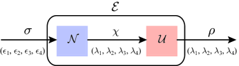
Figure 1: (color online). Modelling the generation of two-qubit states $\rho$ from $\sigma$ through a doubly stochastic process.

Now, for a general realization of the process $\sigma\to\rho$, the generated density matrix $\rho$ can be thought of as arising from a process ${\cal N}$, that can have a non-unitary part, followed by a unitary-only process ${\cal U}$, as depicted in Fig. 1. This means that we have $\sigma\rightarrow\chi\equiv{\mathcal{N}}(\sigma)\rightarrow\rho\equiv{\mathcal{U}}(\chi)$. The process ${\mathcal{N}}$ generates the two-qubit state $\chi$ with eigenvalues $\{\lambda_{1},\lambda_{2},\lambda_{3},\lambda_{4}\}$ which are different from the eigenvalues $\{{\epsilon_{1},\epsilon_{2},\epsilon_{3},\epsilon_{4}}\}$ of $\sigma$, except when $\mathcal{N}$ consists of unitary-only transformations, in which case the eigenvalues of $\chi$ remain the same as that of $\sigma$. The unitary part ${\mathcal{U}}$ transforms the two-qubit state $\chi$ to the final two-qubit state $\rho$. This action does not change the eigenvalues but can change the concurrence of the two-qubit state. The majorization relations of Eq. (6) dictate how the two sets of eigenvalues are related and thus quantify the effects due to $\mathcal{N}$. We quantify the effects due to $\mathcal{U}$ by using the result from Refs. ishizaka2000pra ; verstraete2001pra ; wootters2001qic for the maximum concurrence achievable by a two-qubit state under unitary transformations. According to this result, for a two-qubit state $\rho$ with eigenvalues in non-ascending order denoted as $\lambda_{1},\lambda_{2},\lambda_{3},\lambda_{4}$, the concurrence $C(\rho)$ obeys the inequality:

$$C(\rho)\leq\mathrm{max}\{0,\lambda_{1}-\lambda_{3}-2\sqrt{\lambda_{2}\lambda_{4}}\};$$ (7)

the bound is saturable in the sense that there always exists a unitary transformation $\mathcal{U}(\chi)=\rho$ for which the equality holds true verstraete2001pra . Now, from Eq. (7), we clearly have $C(\rho)\leq\lambda_{1}$. And, from the majorization relation of Eq. (6a), we find that $\lambda_{1}\leq\epsilon_{1}=(1+P)/2$. Therefore, for a general doubly-stochastic process $\mathcal{E}$, we arrive at the inequality:

$$C(\rho)\leq\frac{1+P}{2}.$$ (8)

We stress that this bound is tight, in the sense that there always exists a pair of $\mathcal{N}$ and $\mathcal{U}$ for which the equality in the above equation holds true. In fact, the saturation of Eq.(8) is achieved when $\mathcal{N}$ consists of unitary-only process and when $\mathcal{U}$ is such that it yields the maximum concurrence for $\rho$ as allowed by Eq. (7). This can be verified, first, by noting that when $\mathcal{N}$ is unitary the process $\chi=\mathcal{N}(\sigma)$ preserves the eigenvalues to yield $\left(\lambda_{1},\lambda_{2},\lambda_{3},\lambda_{4}\right)=\left((1+P)/2,(1-P)/2,0,0\right)$, and second, by substituting these eigenvalues in Eq.(7) which then yields $(1+P)/2$ as the maximum achievable concurrence. Eq.(8) is the central result of this Letter which clearly states that the intrinsic polarization correlations of the pump field in PDC predetermine the maximum entanglement that can be achieved by the generated two-qubit signal-idler states. We note that while Eq.(8) has been derived keeping in mind the physical context of parametric down-conversion, the derivation does not make any specific reference to the PDC process or to any explicit details of the two-qubit generation scheme. As a result, Eq.(8) is also applicable to processes other than PDC that would produce a two-qubit state from a single source qubit state via a doubly stochastic process.

We now recall that our present work is directly motivated by previous studies in the spatial degree of freedom for two-qubit states with only two nonzero diagonal entries in the computational basis jha2010pra . Therefore, we next consider this special class of two-qubit states in the polarization degree of freedom. We refer to such states as ‘2D states’ in this Letter and represent the corresponding density matrix as $\rho^{\rm(2D)}$. Since such states can only have two nonzero eigenvalues, the majorization relations of Eq.(6) reduce to: $\lambda_{1}\leq\epsilon_{1}$ and $\lambda_{1}+\lambda_{2}=\epsilon_{1}+\epsilon_{2}=1$. Owing to its $2\times 2$ structure, the state $\rho^{\rm(2D)}$ has a decomposition of the form mandel&wolf ,

$$\rho^{\rm(2D)}=\tilde{P}|\psi^{\rm(2D)}\rangle\langle\psi^{\rm(2D)}|+(1-\tilde{P})\bar{\mathds{1}}^{\rm(2D)},$$ (9)

where $|\psi^{\rm(2D)}\rangle$ is a pure state and $\bar{\mathds{1}}^{\rm(2D)}$ is a normalized $2\times 2$ identity matrix. As in Eq.(2), the pure state weightage $\tilde{P}$ can be shown to be related to the eigenvalues as $\tilde{P}=\lambda_{1}-\lambda_{2}$. It is known that the concurrence is a convex function on the space of density matrices wootters1998prl , that is, $C(\sum_{i}p_{i}\rho_{i})\leq\sum_{i}p_{i}C(\rho_{i})$, where $0\leq p_{i}\leq 1$ and $\sum_{i}p_{i}=1$. Applying this property to Eq. (9) along with the fact that $C(\bar{\mathds{1}}^{\rm(2D)})=0$, we obtain that the concurrence $C(\rho^{\rm(2D)})$ of a 2D state satisfies $C(\rho^{\rm(2D)})\leq\tilde{P}$. Now since $\tilde{P}=\lambda_{1}-\lambda_{2}=2\lambda_{1}-1$, and $\lambda_{1}\leq\epsilon_{1}$, we get $\tilde{P}\leq 2\epsilon_{1}-1=\epsilon_{1}-\epsilon_{2}=P$, or $\tilde{P}\leq P$. We therefore arrive at the inequality,

$$C(\rho^{\rm(2D)})\leq P.$$ (10)

Thus, for 2D states the upper bound on concurrence is the degree of polarization itself. This particular result is in exact analogy with the result shown previously for 2D states in the spatial degree of freedom that the maximum achievable concurrence is bounded by the degree of spatial correlations of the pump field itself.jha2010pra .

Our entire analysis leading upto Eq. (8) and Eq. (10) describes the transfer of one-particle correlations, as quantified by $P$, to two-particle correlations and their eventual manifestation as entanglement, as quantified by concurrence. For 2D states, which have a restricted Hilbert space available to them, the maximum concurrence that can get manifested is $P$. Thus, restricting the Hilbert space appears to restrict the degree to which pump correlations can manifest as the entanglement of the generated two-qubit state. However, when there are no restrictions on the available Hilbert space, the maximum concurrence that can get manifested is $(1+P)/2$.

Next, for conceptual clarity, we illustrate the bounds derived in this Letter in an example experimental scheme shown in Fig. 2(a). This scheme can produce a wide range of two-qubit states in a doubly-stochastic manner. A pump field with the degree of polarization $P$ is split into two arms by a non-polarizing beam-splitter (BS) with splitting ratio $t:1-t$. We represent the horizontal and vertical polarization components of the field hitting the PDC crystals in arm (1) as $E_{H1}$ and $E_{V1}$, respectively. The phase retarder (PR1) introduces a phase difference $\alpha_{1}$ between $E_{H1}$ and $E_{V1}$. The rotation plate (RP1) rotates the polarization vector by angle $\theta_{1}$. The corresponding quantities in arm (2) have similar representations. The stochastic variable $\gamma$ introduces a decoherence between the pump fields in the two arms. Its action is described as $\langle e^{i\gamma}\rangle=\mu\,e^{i\gamma_{0}}$, where $\langle\cdots\rangle$ represents the ensemble average, $\mu$ is the degree of coherence and $\gamma_{0}$ is the mean value of $\gamma$ mandel&wolf . The entangled photons in each arm are produced using type-I PDC in a two-crystal geometry kwiat1999pra . The purpose of the half-wave plate (HP) is to convert the two-photon state vectors $|H\rangle_{s}|H\rangle_{i}$ and $|V\rangle_{s}|V\rangle_{i}$, into $|V\rangle_{s}|H\rangle_{i}$ and $|H\rangle_{s}|V\rangle_{i}$, respectively. Therefore, a typical realization $|\psi_{\gamma}\rangle$ of the two-qubit state in the ensemble detected at $\mathrm{D}_{s}$ and $\mathrm{D}_{i}$ can be represented as $|\psi_{\gamma}\rangle=E_{V1}|H\rangle_{s}|H\rangle_{i}+E_{H1}|V\rangle_{s}|V\rangle_{i}+e^{i\gamma}\left(E_{V2}|H\rangle_{s}|V\rangle_{i}+E_{H2}|V\rangle_{s}|H\rangle_{i}\right)$. The two-qubit density matrix is then $\rho=\langle|\psi_{\gamma}\rangle\langle\psi_{\gamma}|\rangle=$

$$\!\begin{bmatrix}\langle E_{V1}E^{*}_{V1}\rangle&\langle E_{V1}E^{*}_{V2}e^{-i\gamma}\rangle&\langle E_{V1}E^{*}_{H2}e^{-i\gamma}\rangle&\langle E_{V1}E^{*}_{H1}\rangle\\[4.0pt] \langle E_{V2}E^{*}_{V1}e^{i\gamma}\rangle&\langle E_{V2}E^{*}_{V2}\rangle&\langle E_{V2}E^{*}_{H2}\rangle&\langle E_{V2}E^{*}_{H1}e^{i\gamma}\rangle\\[4.0pt] \langle E_{H2}E^{*}_{V1}e^{i\gamma}\rangle&\langle E_{H2}E^{*}_{V2}\rangle&\langle E_{H2}E^{*}_{H2}\rangle&\langle E_{H2}E^{*}_{H1}e^{i\gamma}\rangle\\[4.0pt] \langle E_{H1}E^{*}_{V1}\rangle&\langle E_{H1}E^{*}_{V2}e^{-i\gamma}\rangle&\langle E_{H1}E^{*}_{H2}e^{-i\gamma}\rangle&\langle E_{H1}E^{*}_{H1}\rangle\end{bmatrix}\,.$$

For calculating the matrix elements of $\rho$, we represent the polarization vector of the pump field before the BS as $\left(E_{H},E_{V}\right)^{T}$ and thus write $E_{H1}$ and $E_{V1}$ as

$$\begin{bmatrix}\!E_{H1}\\ E_{V1}\end{bmatrix}\!=\!\eta_{1}\!\begin{bmatrix}\!\cos{\theta_{1}}&\sin{\theta_{1}}\\ -\sin{\theta_{1}}&\cos{\theta_{1}}\!\end{bmatrix}\!\begin{bmatrix}1&0\\ 0&e^{i\alpha_{1}}\end{bmatrix}\!\begin{bmatrix}E_{H}\\ E_{V}\!\end{bmatrix},$$ (11)

where $\eta_{1}=\sqrt{t}$, and the two matrices represent the transformations by PR1 and RP1. $E_{H2}$ and $E_{V2}$ are calculated in a similar manner, with the corresponding quantity $\eta_{2}=\sqrt{1-t}\ e^{i\gamma}$. Without the loss of generality, we assume $\langle E^{*}_{H}E_{H}\rangle=\langle E^{*}_{V}E_{V}\rangle=1/2$ and $\langle E^{*}_{H}E_{V}\rangle=P/2$, and calculate the matrix elements to be

$$\langle E_{V1(2)}E^{*}_{V1(2)}\rangle=|\eta_{1(2)}|^{2}\big{(}1-P\cos\alpha_{1(2)}\sin 2\theta_{1(2)}\big{)}/2,\\ \langle E_{H1(2)}E^{*}_{H1(2)}\rangle=|\eta_{1(2)}|^{2}\big{(}1+P\cos\alpha_{1(2)}\sin 2\theta_{1(2)}\big{)}/2,\\ \hskip 0.56905pt\langle E_{V1(2)}E^{*}_{H1(2)}\rangle=|\eta_{1(2)}|^{2}\,P\big{(}\cos\alpha_{1(2)}\!\cos 2\theta_{1(2)}+i\sin\alpha_{1(2)}\big{)}/2,\\ \langle E_{V1}E^{*}_{V2}e^{-i\gamma}\rangle\!=\!\mu|\eta_{1}\eta_{2}|\big{(}\sin{\theta_{1}}\sin{\theta_{2}}+\cos{\theta_{1}}\cos{\theta_{2}}e^{i(\alpha_{1}-\alpha_{2})}\big{.}\\ \big{.}-P\cos{\theta_{1}}\sin{\theta_{2}}e^{i\alpha_{1}}-P\sin{\theta_{1}}\cos{\theta_{2}}e^{-i\alpha_{2}}\big{)}e^{-i\gamma_{0}}/2,\\ \langle E_{V1}E^{*}_{H2}e^{-i\gamma}\rangle\!=\!\mu|\eta_{1}\eta_{2}|\big{(}-\sin{\theta_{1}}\cos{\theta_{2}}+\cos{\theta_{1}}\sin{\theta_{2}}e^{i(\alpha_{1}-\alpha_{2})}\big{.}\\ \big{.}+P\cos{\theta_{1}}\cos{\theta_{2}}e^{i\alpha_{1}}-P\sin{\theta_{1}}\sin{\theta_{2}}e^{-i\alpha_{2}}\big{)}e^{-i\gamma_{0}}/2,\\ \langle E_{V2}E^{*}_{H1}e^{i\gamma}\rangle\!=\!\mu|\eta_{1}\eta_{2}|\big{(}-\cos{\theta_{1}}\sin{\theta_{2}}+\sin{\theta_{1}}\cos{\theta_{2}}e^{-i(\alpha_{1}-\alpha_{2})}\big{.}\\ \big{.}-P\sin{\theta_{1}}\sin{\theta_{2}}e^{-i\alpha_{1}}+P\cos{\theta_{1}}\cos{\theta_{2}}e^{i\alpha_{2}}\big{)}e^{i\gamma_{0}}/2,\\ \langle E_{H2}E^{*}_{H1}e^{i\gamma}\rangle\!=\!\mu|\eta_{1}\eta_{2}|\big{(}\cos{\theta_{1}}\cos{\theta_{2}}+\sin{\theta_{1}}\sin{\theta_{2}}e^{-i(\alpha_{1}-\alpha_{2})}\big{.}\\ \big{.}+P\sin{\theta_{1}}\cos{\theta_{2}}e^{-i\alpha_{1}}+P\cos{\theta_{1}}\sin{\theta_{2}}e^{i\alpha_{2}}\big{)}e^{i\gamma_{0}}/2.$$

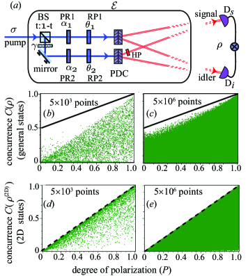
Figure 2: (color online). (a) An example experimental scheme for producing a wide range of two-qubit states. BS: beam-splitter, PR: phase retarder, RP: rotation plate, HP: half-wave plate; $\mathrm{D}_{s}$ and $\mathrm{D}_{i}$ are photon detectors in a coincidence-counting setup. (b) and (c) are the scatter plots of concurrences of states numerically generated by randomly varying all the tunable parameters. (d) and (e) are the scatter plots of concurrence of 2D states, numerically generated by keeping $t=1$ and varying all the remaining tunable parameters.

Here, $t,\alpha_{1},\alpha_{2},\theta_{1},\theta_{2}$, $\mu$, and $\gamma_{0}$ are the tunable parameters. We numerically vary these parameters with a uniform random sampling and simulate a large number of two-qubit states. Fig.2(b) and Fig. 2(c) are the scatter plots of concurrences of $5\times 10^{3}$ and $5\times 10^{6}$ two-qubit states, respectively, numerically generated by varying all the tunable parameters. Fig.2(d) and Fig. 2(e) are the scatter plots of concurrence of $5\times 10^{3}$ and $5\times 10^{6}$ 2D states, respectively, numerically generated by keeping $t=1$ and varying all the remaining tunable parameters. The solid black lines are the general upper bound $C(\rho)=(1+P)/2$ and the dashed black lines are the upper bound $C(\rho)=P$ for 2D states. The unfilled gaps in the scatter plots can be filled in either by sampling more data points or by adopting a different sampling strategy. To this end, we note that one possible setting for which the general upper bound can be achieved is: $t=0.5,\theta_{1}=-\pi/4,\theta_{2}=0,\alpha_{1}=\pi/2,\alpha_{2}=\pi,\mu=1$ and $\gamma_{0}=0$.

In conclusion, we have investigated how one-particle correlations transfer to manifest as two-particle correlations in the physical context of PDC. We have shown that if the generation process is trace-preserving and entropy-nondecreasing, the concurrence $C(\rho)$ of the generated two-qubit state $\rho$ follows an intrinsic upper bound with $C(\rho)\leq(1+P)/2$, where $P$ is the degree of polarization of the pump photon. For the special class of two-qubit states $\rho^{\rm(2D)}$ that is restricted to have only two nonzero diagonal elements, the upper bound on concurrence is the degree of polarization itself, that is, $C(\rho^{\rm(2D)})\leq P$. The surplus of $(1+P)/2-P=(1-P)/2$ in the maximum achievable concurrence for arbitrary two-qubit states can be attributed to the availability of the entire $4\times 4$ computational space, as opposed to 2D states which only have a $2\times 2$ computational block available to them. We believe these results can have two important implications. The first one is to understand from a fundamental perspective, whether or not correlations too follow a quantifiable conservation principle just as physical observables such as energy, momentum do. The second one is that this formalism provides a systematic method of deducing an upper bound on the correlations in a generated quantum system, purely from the knowledge of the correlations of the source. In the light of the recent experiment on generation of three-photon entangled states from a single source photon hamel2014natphoto , this formalism may prove useful in determining upper bounds on the entanglement of such multipartite systems, for which no well-accepted measure exists. This alternative approach based on intrinsic source correlations could complement the existing information-theoretic approaches bennett1996pra ; bennett1996pra2 ; bennett1996prl ; popescu1997pra ; wootters2001qic ; hill1997prl ; wootters1998prl ; nielsen1999prl ; torres2015prl towards quantifying entanglement.

GK acknowledges helpful discussions on the Physics StackExchange online forum. AKJ acknowledges financial support through an initiation grant from IIT Kanpur.

References

- (1) L. Mandel and E. Wolf, Optical Coherence and Quantum Optics (Cambridge university press, New York, 1995).
- (2) R. J. Glauber, Phys. Rev. 130, 2529 (1963).
- (3) E. C. G. Sudarshan, Phys. Rev. Lett. 10, 277 (1963).
- (4) A. Einstein, B. Podolsky, and N. Rosen, Phys. Rev. 47, 777 (1935).
- (5) E. Schrödinger, Proc. Cambridge Philos. Soc. 31, 555 (1935).
- (6) D. C. Burnham and D. L. Weinberg, Phys. Rev. Lett. 25, 84 (1970).
- (7) R. W. Boyd, Nonlinear Optics, 2nd ed. (Academic Press, New York, 2003).
- (8) A. Mair, A. Vaziri, G. Weihs, and A. Zeilinger, Nature 412, 313 (2001).
- (9) W. Vogel and J. Sperling, Phys. Rev. A 89, 052302 (2014).
- (10) T. Baumgratz, M. Cramer, and M. B. Plenio, Phys. Rev. Lett. 113, 140401 (2014).
- (11) D. Girolami, Phys. Rev. Lett. 113, 170401 (2014).
- (12) A. Streltsov, U. Singh, H. S. Dhar, M. N. Bera, and G. Adesso, Phys. Rev. Lett. 115, 020403 (2015).
- (13) Y. Yao, X. Xiao, L. Ge, and C. P. Sun, Phys. Rev. A 92, 022112 (2015).
- (14) E. Wolf, Introduction to the Theory of Coherence and Polarization of Light (Cambridge University Press, New York, 2007).
- (15) P. G. Kwiat, K. Mattle, H. Weinfurter, A. Zeilinger, A. V. Sergienko, and Y. Shih, Phys. Rev. Lett. 75, 4337 (1995).
- (16) C. H. Bennett, D. P. DiVincenzo, J. A. Smolin, and W. K. Wootters, Phys. Rev. A 54, 3824 (1996).
- (17) C. H. Bennett, H. J. Bernstein, S. Popescu, and B. Schumacher, Phys. Rev. A 53, 2046 (1996).
- (18) C. H. Bennett, G. Brassard, S. Popescu, B. Schumacher, J. A. Smolin, and W. K. Wootters, Phys. Rev. Lett. 76, 722 (1996).
- (19) S. Popescu and D. Rohrlich, Phys. Rev. A 56, R3319 (1997).
- (20) W. K. Wootters, Quantum Information & Computation 1, 27 (2001).
- (21) S. Hill and W. K. Wootters, Phys. Rev. Lett. 78, 5022 (1997).
- (22) W. K. Wootters, Phys. Rev. Lett. 80, 2245 (1998).
- (23) M. A. Nielsen, Phys. Rev. Lett. 83, 436 (1999).
- (24) J. Svozilík, A. Vallés, J. Peřina, and J. P. Torres, Phys. Rev. Lett. 115, 220501 (2015).
- (25) M. Born and E. Wolf, Principles of Optics, 7th expanded ed. (Cambridge University Press, Cambridge, 1999).
- (26) A. K. Jha, M. N. O’Sullivan, K. W. C. Chan, and R. W. Boyd, Phys. Rev. A 77, 021801 (2008).
- (27) A. K. Jha and R. W. Boyd, Phys. Rev. A 81, 013828 (2010).
- (28) A. K. Jha, J. Leach, B. Jack, S. Franke-Arnold, S. M. Barnett, R. W. Boyd, and M. J. Padgett, Phys. Rev. Lett. 104, 010501 (2010).
- (29) C. H. Monken, P. H. S. Ribeiro, and S. Pádua, Phys. Rev. A 57, 3123 (1998).
- (30) M. A. Olvera and S. Franke-Arnold, arXiv preprint arXiv:1507.08623 (2015).
- (31) R. Bhatia, Matrix analysis (Springer Science & Business Media, New York, 2013).
- (32) M. A. Nielsen and I. L. Chuang, Quantum computation and quantum information (Cambridge university press, New York, 2010).
- (33) E. C. G. Sudarshan, P. M. Mathews, and J. Rau, Phys. Rev. 121, 920 (1961).
- (34) T. F. Jordan and E. Sudarshan, Journal of Mathematical Physics 2, 772 (1961).
- (35) K. Kraus, Annals of Physics 64, 311 (1971).
- (36) M. A. Nielsen, Lecture Notes, Department of Physics, University of Queensland, Australia (2002).
- (37) S. Ishizaka and T. Hiroshima, Phys. Rev. A 62, 022310 (2000).
- (38) F. Verstraete, K. Audenaert, and B. De Moor, Phys. Rev. A 64, 012316 (2001).
- (39) P. G. Kwiat, E. Waks, A. G. White, I. Appelbaum, and P. H. Eberhard, Phys. Rev. A 60, R773 (1999).
- (40) D. R. Hamel, L. K. Shalm, H. Hübel, A. J. Miller, F. Marsili, V. B. Verma, R. P. Mirin, S. W. Nam, K. J. Resch, and T. Jennewein, Nature Photonics 8, 801 (2014).