Broadband linear polarization of Jupiter Trojans

Abstract

Context. Trojan asteroids orbit in the Lagrange points of the system Sun-planet-asteroid. Their dynamical stability make their physical properties important proxies for the early evolution of our solar system.

Aims. To study their origin, we want to characterize the surfaces of Jupiter Trojan asteroids and check possible similarities with objects of the main belt and of the Kuiper Belt.

Methods. We have obtained high-accuracy broad-band linear polarization measurements of six Jupiter Trojans of the L4 population and tried to estimate the main features of their polarimetric behaviour. We have compared the polarimetric properties of our targets among themselves, and with those of other atmosphere-less bodies of our solar system.

Results. Our sample show approximately homogeneous polarimetric behaviour, although some distinct features are found between them. In general, the polarimetric properties of Trojan asteroids are similar to those of D- and P-type main-belt asteroids. No sign of coma activity is detected in any of the observed objects.

Conclusions. An extended polarimetric survey may help to further investigate the origin and the surface evolution of Jupiter Trojans.

1 Introduction

Trojan asteroids are confined by solar and planetary gravity to orbiting the Sun 60° ahead (L4 Lagrange point of the binary system planet Sun) or behind (L5 Lagrange point) a planet’s position along its orbit (Murray & Dermott 1999). Stable trojans are supported by Mars, by Jupiter, by Neptune, and by two Saturnian moons. Because of their dynamical stability, they allow us to look at the earliest stages of the formation of our solar system. Saturn and Uranus do not have a stable Trojan population because their orbits are perturbed on a short time scale compared to the age of the solar system. Terrestrial planets may support a population of Trojan asteroids, (e.g. the Earth Trojan 2010 TK₇ discovered by Connors et al. 2011), but so far no stable population has been identified.

More than 6000 Trojans of Jupiter are known so far (Emery et al. 2015). In the framework of the Nice model of the formation of our solar system, Morbidelli et al. (2005) predicted the capture of Jupiter Trojans from the proto Kuiper belt. While these predictions were invalidated by further simulations (e.g. Nesvorný & Morbidelli 2012), Nesvorný et al. (2013) investigated the possibility of the capture of Jupiter Trojans from the Kuiper-belt region within the framework of the so-called jumping-Jupiter scenario, and succeeded at reproducing the observed distribution of the orbital elements of Jupiter Trojan asteroids. The model by Nesvorný et al. (2013) supports the scenario in which the majority of Trojans are captured from the trans-Neptunian disk, while a small fraction of them may come from the outer asteroid belt.

Unfortunately, direct spectral comparisons between the optical properties of Jupiter Trojans with those of Kuiper-belt objects (or trans-Neptunian objects, TNOs) show significant differences. TNOs have a wide range of albedos that extend, in particular, to higher albedos, while all known Jupiter Trojans have a low albedo and fairly featureless spectrum, all belonging to ‘primitive’ taxonomies, principally C-, D-, and P-types of the Tholen (Tholen 1984) classification system (Grav et al. 2012). These types are the most common ones in the outer part of the main belt.

Emery et al. (2011) investigated the infrared properties of Jupiter Trojans and report a bimodal distribution of their spectral slopes. This bimodality is also seen in the albedos in the infrared (Grav et al. 2012), although it is not apparent in the optical albedo distribution. Emery et al. (2011) interpret the slope bimodality as the observational evidence of at least two distinct populations of objects within the Trojan clouds where the ‘less red’ group originated near Jupiter (i.e. either at Jupiter’s radial distance from the Sun or in the Main Asteroid Belt), while the ‘redder’ population originated significantly beyond Jupiter’s orbit (where similar ‘red’ objects are prevalent). Therefore, at least the near-IR spectroscopy observations of Emery et al. (2011) are broadly consistent with the widely accepted scenario suggested by Morbidelli et al. (2005) and Nesvorný et al. (2013), while the inconsistency in the optical albedo and spectral properties could be naturally explained by the fact that TNOs migrated to the Jupiter orbit have been exposed to a different irradiation and thermal environment (Emery et al. 2015).

Polarimetric measurements are sensitive to the micro-structure and composition of a scattering surface. In the case of the atmosphere-less bodies of the solar system, the way that linear polarization changes as a function of the phase angle (i.e., the angle between the sun, the target, and the observer) may reveal information about the properties of the topmost surface layers, such as the complex refractive index, particle size, packing density, and microscopic optical heterogeneity. Objects that display different polarimetric behaviours must have different surface structures, so that they probably have different evolution histories. Polarimetric techniques have been applied to hundreds of asteroids (e.g., Belskaya et al. 2015), as well as to a few Centaurs (Bagnulo et al. 2006; Belskaya et al. 2010) and TNOs (Boehnhardt et al. 2004; Bagnulo et al. 2006, 2008; Belskaya et al. 2010). These works have revealed that certain objects exhibit very distinct polarimetric features. For instances, at very small phase angles, some TNOs and Centaurs exhibit a very steep polarimetric curve that is not observed in main-belt asteroids. This finding is evidence of substantial differences in the surface micro-structure of these bodies compared to other bodies in the inner part of the solar system. It is therefore very natural to explore whether optical polarimetry may help in finding other similarities or differences among Jupiter Trojans, and between Jupiter Trojans and other classes of solar system objects.

In this work, we carry out a pilot study intending to explore whether polarimetry can bring additional constraints that help to understand the origin and the composition of Jupiter Trojans better. We present polarimetric observations of six objects belonging to the L4 Jupiter Trojan population: (588) Achilles, (1583) Antilochus, (3548) Eurybates, (4543) Phoinix, (6545) 1986 TR6, and (21601) 1998 XO89. All our targets have sizes in the diameter range of 50–160 km, and represent both spectral groups defined by Emery et al. (2011).

From ground-based facilities, Jupiter Trojans may be observed up to a maximum phase-angle of $\sim 12\degr$. Our observations cover the range $7\degr-12\degr$ and are characterized by a ultra-high signal-to-noise ratio (S/N) of $\sim 5000$, so their accuracy is not limited by photon noise, but by instrumental polarization and other systematic effects. Our observations are aimed at directly addressing the question of how diverse the polarimetric properties of the L4 population of Trojans are and how they compare with the polarimetric properties of other objects of the solar system. With our data we can estimate the minimum of their polarization curves and make a comparison with the behaviour of low-albedo main-belt asteroids. Finally, by combining the polarimetric images, we can also try to detect coma activity (if any) with great precision.

2 Observations and results

Table 1: Polarimetry and photometry of six Jupiter Trojans asteroids in the special $R$ FORS filter. $P_{Q}$ and $P_{U}$ are the reduced Stokes parameters measured in a reference system such that $P_{Q}$ is the flux perpendicular to the plane Sun-Object-Earth (the scattering plane) minus the flux parallel to that plane, divided by the sum of the two fluxes. Null parameters $N_{Q}$ and $N_{U}$ are expected to be zero within error bars. $m_{R}$ is the observed magnitude in the $R$ filter, and $R(1,1,\alpha)$ is the magnitude as if the object was observed at geocentric and heliocentric distances = 1 au at phase angle $\alpha$. Photometric error bars are estimated a priori = 0.05.

				Phase
	Time	Exp		angle $\alpha$	$P_{Q}$		$N_{Q}$	$P_{U}$		$N_{U}$
Date	(UT)	(sec)	OBJECT	(°)	(%)		(%)	(%)		(%)	$m_{R}$	$R(1,1,\alpha)$
2013 04 12	04:40	400	588	9.31	$-$1.07 $\pm$	0.02	$-$0.02	0.01 $\pm$	0.02	$-$0.04	$14.92$	$8.39$
2013 04 18	01:16	96	Achilles	10.03	$-$1.07 $\pm$	0.04	0.00	$-$0.07 $\pm$	0.04	$-$0.06	$15.00$	$8.43$
2013 05 26	01:33	680	(1906 TG)	11.93	$-$0.98 $\pm$	0.03	$-$0.02	$-$0.01 $\pm$	0.03	0.01	$\leq 15.59$	$\leq 8.62$
2013 04 11	02:26	560	1583	9.15	$-$1.22 $\pm$	0.02	0.02	$-$0.01 $\pm$	0.02	$-$0.01	$15.74$	$8.87$
2013 04 18	04:13	480	Antilochus	9.75	$-$1.23 $\pm$	0.03	$-$0.01	0.01 $\pm$	0.03	0.02	$15.89$	$8.98$
2013 05 13	00:52	400	(1950 SA)	11.07	$-$1.25 $\pm$	0.03	0.00	0.00 $\pm$	0.03	0.02	$15.96$	$8.90$
2013 04 12	03:31	1280	3548	7.35	$-$1.18 $\pm$	0.03	$-$0.02	$-$0.04 $\pm$	0.03	0.03	$16.73$	$9.93$
2013 04 18	03:41	1450	Eurybates	8.21	$-$1.25 $\pm$	0.03	$-$0.05	$-$0.04 $\pm$	0.03	0.03	$16.78$	$9.95$
2013 04 19	04:31	1420	(1973 SO)	8.35	$-$1.31 $\pm$	0.03	$-$0.03	0.02 $\pm$	0.03	$-$0.04	$16.72$	$9.88$
2013 06 01	01:30	1760		11.18	$-$1.28 $\pm$	0.04	0.00	0.03 $\pm$	0.04	$-$0.08	$\leq 17.29$	$\leq 10.16$
2013 04 11	03:00	1440	4543	7.32	$-$0.91 $\pm$	0.03	$-$0.02	0.00 $\pm$	0.03	$-$0.02	$\leq 16.71$	$\leq 9.82$
2013 04 19	01:24	1660	Phoinix	8.40	$-$0.91 $\pm$	0.03	0.02	$-$0.02 $\pm$	0.03	0.01	$16.78$	$9.85$
2013 06 04	01:56	1920	(1989 CQ1)	10.96	$-$0.97 $\pm$	0.03	$-$0.02	0.04 $\pm$	0.03	$-$0.02	$17.39$	$10.14$
2013 04 12	04:08	1080	6545	8.79	$-$1.20 $\pm$	0.03	0.03	0.02 $\pm$	0.03	$-$0.04	$17.24$	$10.43$
2013 04 25	02:58	2400	(1986 TR6)	10.13	$-$1.04 $\pm$	0.09	0.07	0.11 $\pm$	0.10	$-$0.01	$\leq 17.37$	$\leq 10.49$
2013 06 05	01:25	2400		11.14	$-$1.25 $\pm$	0.04	0.07	0.02 $\pm$	0.04	$-$0.01	$17.81$	$10.64$
2013 04 11	03:40	1360	21601	6.83	$-$1.17 $\pm$	0.03	0.02	$-$0.02 $\pm$	0.03	$-$0.01	$16.84$	$10.14$
2013 04 19	05:10	1390	(1998 X089)	7.85	$-$1.18 $\pm$	0.03	0.11	0.01 $\pm$	0.03	$-$0.06	$16.93$	$10.20$
2013 05 26	02:27	1920		11.07	$-$1.13 $\pm$	0.09	0.10	$-$0.07 $\pm$	0.09	$-$0.01	$\leq 17.67$	$\leq 10.72$
2013 06 05	02:20	1920		11.36	$-$1.19 $\pm$	0.03	$-$0.05	0.04 $\pm$	0.03	0.05	$17.59$	$10.58$

Our observations were obtained with the FORS2 instrument (Appenzeller & Rupprecht 1992; Appenzeller et al. 1998) of the ESO VLT using the well-established beam-swapping technique (e.g. Bagnulo et al. 2009), setting the retarder waveplate at 0°, 22.5°, …,157.5°. For each observing series, the exposure time accumulated over all exposures varied from a few minutes for (588) Achilles up to 40 minutes for (6545) 1986 TR6.

2.1 Instrument setting

Jupiter Trojans are relatively bright targets for the VLT, therefore the S/N may be limited by the number of photons that can be measured with the instrument CCD without reaching saturation, rather than by mirror size and shutter time. The telescope time requested to reach an ultra-high S/N is in part determined by overheads for CCD readout. The standard readout mode of the FORS CCD has a conversion factor from e^- to ADU of 1.25 and 2$\times$2 binning readout mode. Each pixel size, after rebinning, corresponds to 0.25″. Therefore, for a 1″ seeing, the $2^{16}-1$ maximum ADU counts set by the ADC converter limits the S/N achievable with each frame to $\sim 1000-1400$ (neglecting background noise and taking into account that the incoming radiation is split into two beams). To increase the efficiency, we requested the use of a non-standard $1\times 1$ readout mode for our observing run. This way, pixel size was reduced to 0.125″, and with a conversion factor of ADU to e^- of 1.25, we could expect to reach a S/N per frame of $\sim 2000-2800$. We also requested special sky flat fields obtained with the same readout mode. While flat-fielding is not a necessary step for the polarimetry of bright objects, we found that it improved the quality of our results because it reduces the noise introduced by background subtraction. For consistency with previous FORS measurements of Centaurs and TNO, our broadband linear polarization measurements were obtained in the $R$ filter.

2.2 Aperture polarimetry

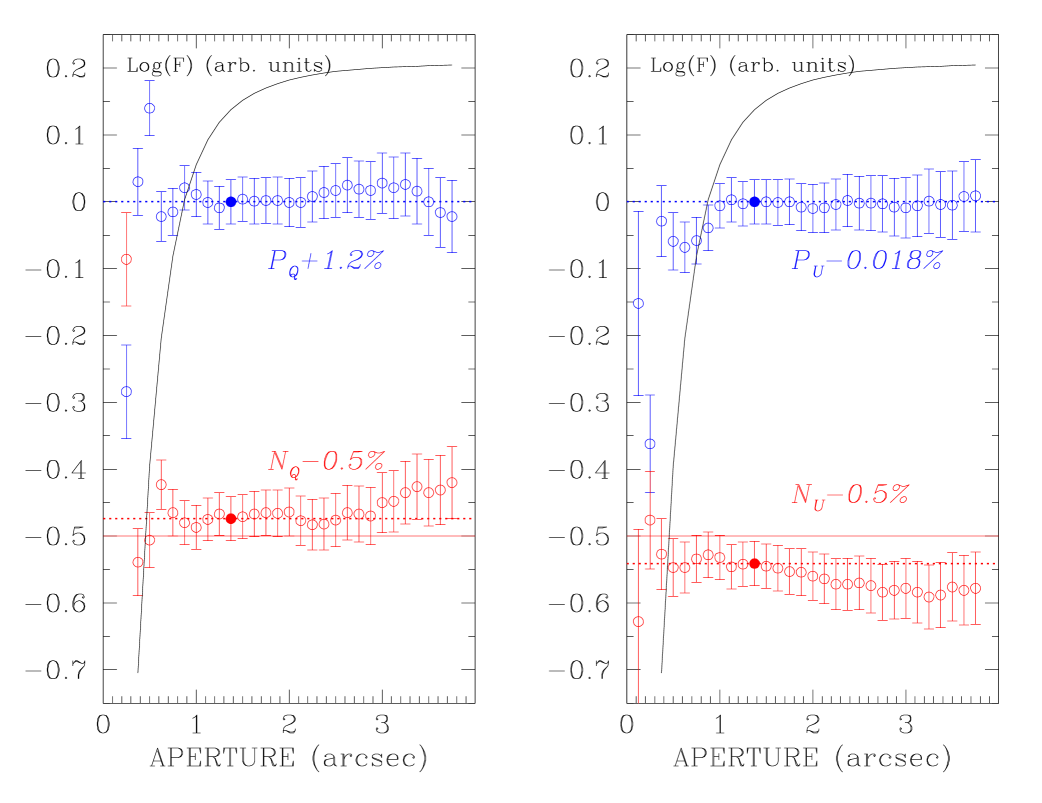
Figure 1: The principle of aperture polarimetry. The Figure is explained in the text (Sect. 2.2 and 2.2.1).

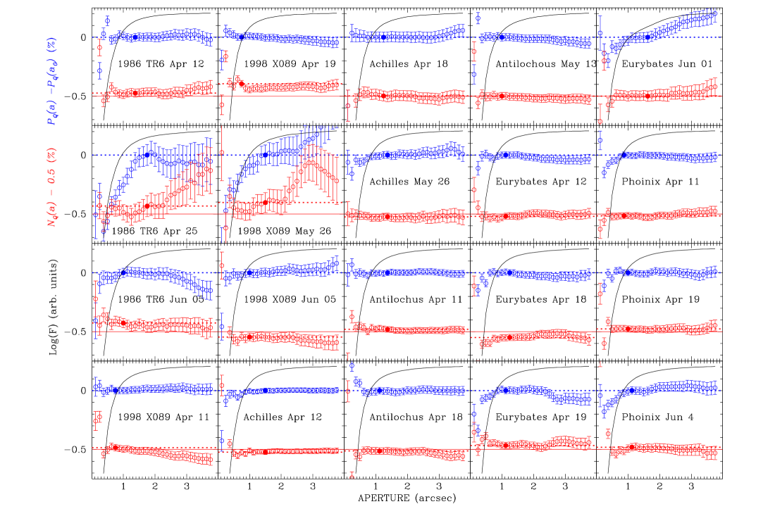
Figure 9: Aperture polarimetry: $P_{Q}$ and $N_{Q}$ parameters as function of the aperture for the various observing series. $P_{Q}$ parameters, represented by blue empty circles, are offset to the values corresponding to the aperture adopted for the measurement and reported in Table 1. This point is hightlighted with solid circles and dotted lines. $N_{Q}$ parameters, represented by red empty circles, are offset by $-0.5$ % for display purpose. Again, the adopted values are highlighted with solid symbols and dotted lines. Each panel of this figure is similar to the left panel of Fig.1 and is explained in more detail in Sect. 2.2.

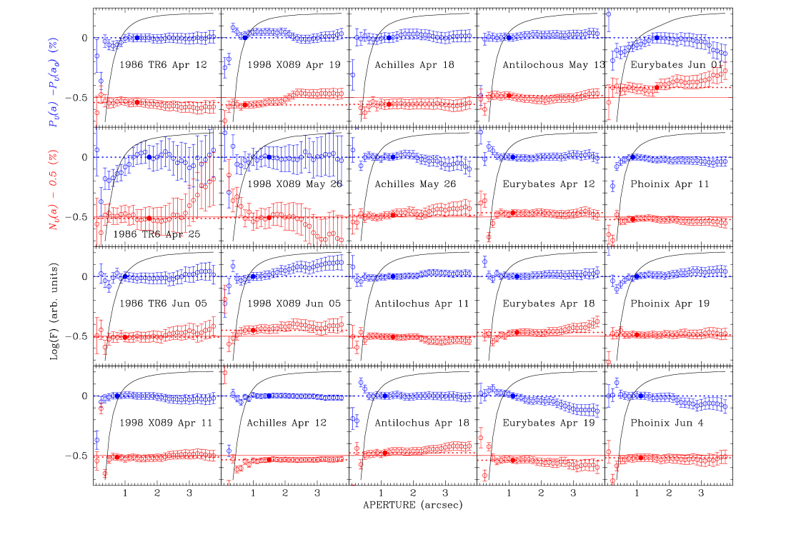
Figure 10: Aperture polarimetry: $P_{U}$ and $N_{U}$ parameters as function of the aperture for the various observing series. $P_{U}$ parameters, represented by blue empty circles, are offset to the value corresponding to the aperture adopted for the measurement and reported in Table 1. This point is hightlighted with solid circles and dotted lines. $N_{Q}$ parameters are represented by red empty circles, and are offset by $-0.5$ % for display purpose. Again, the adopted values are highlighted with solid symbols and dotted lines. Each panel of this figure is similar to the right panel of Fig.1 and is explained in more detail in Sect. 2.2.

Fluxes were calculated for apertures up to a 30-pixel radius (=3.75″) with one-pixel (=0.125″) increments. Sky background was generally calculated in an annulus with inner and outer radii of 28 and 58 pixels (i.e. 4.5″and 7.25″), respectively. Imaging aperture polarimetry was performed as explained in Bagnulo et al. (2011) by selecting the aperture at which the reduced Stokes paremeters $P_{Q}=Q/I$ and $P_{U}=U/I$ converge to a well-defined value. Polarimetric measurements are reported the perpendicular to the great circle passing through the object and the Sun adopting as a reference direction. This way, $P_{Q}$ represents the flux perpendicular to the plane Sun-object-Earth (the scattering plane) minus the flux parallel to that plane, divided by the sum of these fluxes. For symmetry reasons, $P_{U}$ values are always expected to be zero, and inspecting their values allows us to perform an indirect quality check of the $P_{Q}$ values. This “growth-curve” method is illustrated in Fig. 1 for one individual case, while Figs. 9 and 10 (available in the appendix of the online version) show the same plot for all observed targets.

Figures 1, 9, and 10 contain a lot of information, and it is worthwhile commenting on them in detail. In the left-hand panel of Fig. 1, the blue empty circles show the $P_{Q}$ values measured as a function of the aperture used for the flux measurement, with their error bars calculated from photon noise and background subtraction using Eqs. (A3), (A4), and (A11) of Bagnulo et al. (2009). The $P_{Q}$ values are offset to the value adopted in Table 1. Ideally, for apertures slightly larger than the seeing, $P_{Q}$ should converge to a well defined value, that should be adopted as $P_{Q}$ measurement value in Table 1.

Practically speaking, Figs. 1 and 9 clearly show that $P_{Q}$ sometimes depends on the aperture in a complicated way, mainly due to the presence of background objects that enter into the aperture where flux is measured (see e.g. the case of Eurybates observed on June 1 in Figs. 9 and 10.) The values reported in Table 1 were selected through visual inspection of Figs. 9, as the value corresponding to the smallest aperture of a “plateau” of the growth curve rather than to its asymptotic value.

Lower in the figure, the empty red circles show the null parameters offset to the value adopted in Table 1, and offset by $-0.5$ % for display purpose. The solid circle shows the aperture adopted for the $P_{Q}$ measurement, and the corresponding $N_{Q}$ value is shown with a dotted line. In practice, the distances between the solid line at $-0.5$ % and the empty circles correspond to the null parameter values, and the distance between solid line and the dotted line shows the $N_{Q}$ value of Table 1. The physical significance of the null parameters is discussed in Sect. 2.2.1.

The black solid line shows the logarithm of the total flux expressed in arbitrary units. In this context it does not have any diagnostic meaning, but demonstrates that polarimetric measurements converge at lower aperture values than photometry and suggests that simple aperture polarimetry leads to results more robust than those of aperture photometry.

The right-hand panels of Figs. 1 and 10 refer to $P_{U}$ and $N_{U}$and are organized in exactly the same way as the left-hand panels of Figs. 1 and 9, respectively. For quality-check purposes, the aperture of $P_{U}$ was selected to be identical to that of $P_{Q}$ (see Sect. 2.2.2).

2.2.1 Quality checks with the null parameters

The polarimetric measurements presented here were obtained using the so-called beam-swapping technique; i.e., Stokes parameters are obtained as the difference between two observations obtained at position angles of the retarder waveplate separated by 45°. This technique allows one to minimize spurious contributions due to the instrument. For instance, the reduced Stokes parameter $P_{Q}$ was obtained as

$$\frac{1}{2}\left[P_{Q}(\phi=0\degr)+P_{Q}(\phi=90\degr)\right],$$ (1)

where

$$P_{Q}(\phi)=\frac{1}{2}\left[\left(\frac{f^{\parallel}-f^{\perp}}{f^{\parallel}+f^{\perp}}\right)_{\phi}-\left(\frac{f^{\parallel}-f^{\perp}}{f^{\parallel}+f^{\perp}}\right)_{\phi+45\degr}\right],$$ (2)

where $\phi$ is the position angle of the retarder waveplate, and $f^{\parallel}$ ($f^{\perp}$) is the flux measured in the parallel (perpendicular) beam of the retarder waveplate.

The null parameter $N_{Q}$ ($N_{U}$) is defined as the difference between the $P_{Q}$ values obtained from distinct pairs of observations:

$$\frac{1}{2}\left[P_{Q}(\phi=0\degr)-P_{Q}(\phi=90\degr)\right]\;.$$ (3)

Bagnulo et al. (2009) have shown that, in the ideal case, the results of repeated measurements of the null parameters are expected to be scattered about zero according to a Gaussian distribution with the same $\sigma$ as the $P_{Q}$ ($P_{U}$) error bar. (Of course, we do not expect a Gaussian distribution for the $N_{Q}$ values measured on the same frames but with different apertures, since these are not independent measurements.) The consistency of the null parameters with zero within the $P_{Q}$ error bars are therefore an indirect form of quality check. For instance, an $N_{Q}$ value inconsistent with zero could be due to the presence of a cosmic ray, or a background object or reflection in the aperture for some positions of the retarder waveplate. These events would also affect the $P_{Q}$ measurement, therefore one has to be wary of $P_{Q}$ measurements that have high $N_{Q}$ values. Figures 1, 9, and 10 show that the null parameters are scattered about zero well within 2 $\sigma$.

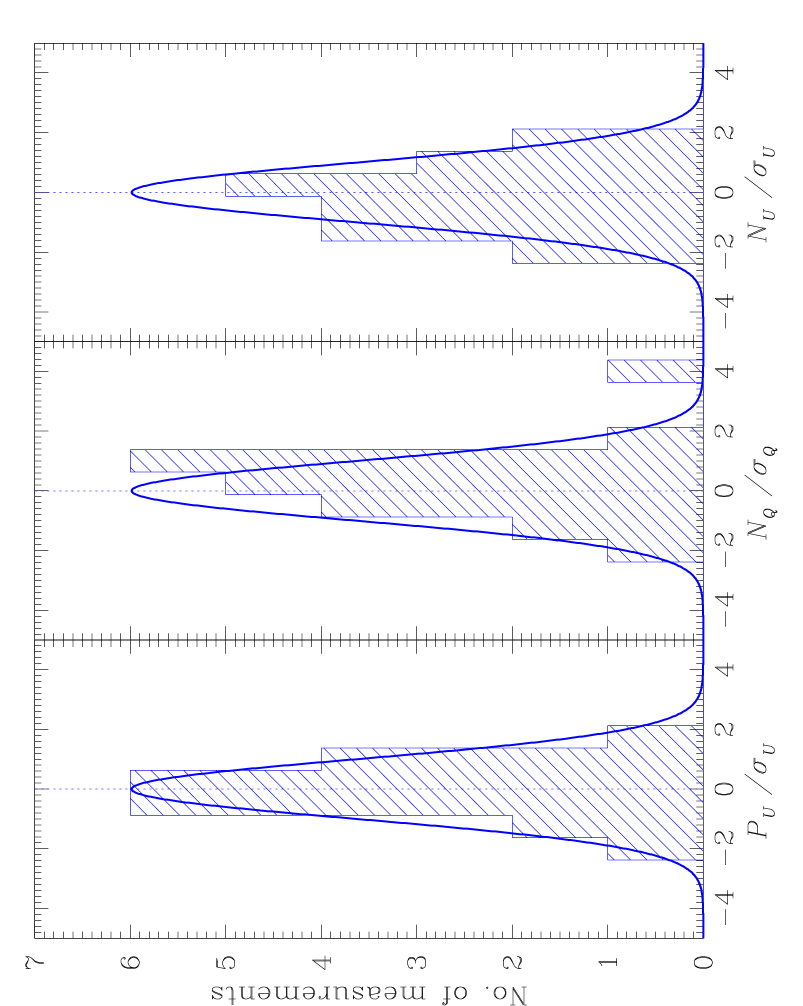
Figure 2: Distribution of the $P_{U}$, $N_{Q}$ and $N_{U}$ parameters normalised by the error bars, compared to a Gaussian with $\sigma=1$.

2.2.2 Quality checks with $P_{U}$

If the target is macroscopically symmetric about the scattering plane, $P_{U}$ is expected to be zero. An individual $P_{U}$ measurement that significantly deviates from zero means either that there is a problem with the measurement (similar to what is discussed for the null parameter) or that the object is not symmetric about the plane identified by the object, the Sun, and the observer. When considering a large sample, all $P_{U}$ measurements of different objects should be scattered around zero. The null parameters should be scattered around zero, and the null parameters normalized by their error bar should be fit by a Gaussian with $\sigma=1$ centred on zero.

Inspection of the distribution of $P_{U}$ parameters initially showed a systematic offset by $\sim-1\,\sigma$. Another way to see exactly the same effect is to calculate the average polarization position angle measured from the perpendicular to the scattering plane: we found 90.4°instead of 90.0°. This 0.4° rotation offset can be easily explained by an imperfect alignment of the polarimetric optics and by an imperfect estimate of the chromatism of the retarder waveplate. To compensate for the waveplate chromatism in the R Bessel filter, we had originally adopted the rotation suggested by the FORS user manual of $-1.2\degr$. After inspecting the $P_{U}$ values, we instead decided to adopt a rotation by $-0.8$°. Figure 2 shows the histograms of the $P_{U}$, $N_{Q}$, and $N_{U}$ values normalized to their error bars. The marginal deviations from the expected Gaussian distribution do not look systematic and may only be ascribed to the sample still being relatively small statistically.

2.3 Aperture photometry

The importance of acquiring simultaneous photometry and polarimetry has probably been underestimated in the past. Modelling attempts need both pieces of information, which are only available for a handful of asteroids. However, at least with certain instrument configurations, photometry may be a by-product of polarimetric measurements. In the case of the FORS instrument, an acquisition image is always obtained prior to inserting the polarimetric optics. This can be used to estimate the absolute brightness of the target, if the observing night is photometric. (In fact, even if this is not the case, one could in principle observe the same field again during a photometric night and calibrate the previous observations). Therefore we performed aperture photometry from our acquisition images, and then we calculated

$$R(r=1\,{\rm au},\Delta=1\,{\rm au},\alpha)=m_{R}-5\,{\rm Log}_{10}\left(r\,\Delta\right)$$

where $r$ and $\Delta$ are the heliocentric and geocentric distances, respectively, and $m_{R}$ is obtained from the instrument magnitude $m_{R}^{\rm(instr)}$ using

$$m_{R}=m_{R}^{\rm(instr)}-k_{R}X-k_{VR}\,(V-R)X+{ZP}_{R}$$

where $ZP_{R}$, $k_{R}$ and $k_{VR}$ are the zero point and the extinction coefficient in the $R$ filter and the $(V-R)$ colour index tabulated in the FORS2 QC1 database, respectively, and $X$ is the airmass. Aperture photometry can also be performed on the images obtained with the polarimetric optics in, if these are calibrated. From a comparison between photometry obtained from the acquisition images and photometry obtained from the polarimetric images (obtained adding $f^{\parallel}$ and $f^{\perp}$), we estimated that zero points of the frames obtained in polarimetric mode with the $R$ special filter can be obtained by subtracting 0.31 from the zero points obtained in imaging mode.

Both $ZP_{R}$ and $k_{VR}$ are night dependent (their values are $\sim 28.28$ and $0.01$, respectively). Based on the night-to-night variations, we a priori assigned an error of 0.05 and 0.0005 to the zero point and to the colour term, respectively. ESO classifies each night with the symbols S(table), U(known), or Non stable. Unfortunately, only three out of our 20 observing series were obtained during stable nights. The reason is that to maximize the chances that our observations would be performed during the desired time windows, we set only loose constraints on sky transparency. However, since we obtained several frames during an extended period of time (typically 30–60 min), it is still possible to roughly evaluate the stability of the atmospheric conditions at the time of our observations. We also note that the Line of Sight Sky Absorption Monitor (LOSSAM, available online through the ESO web site) shows that most of the observing nights were actually clear.

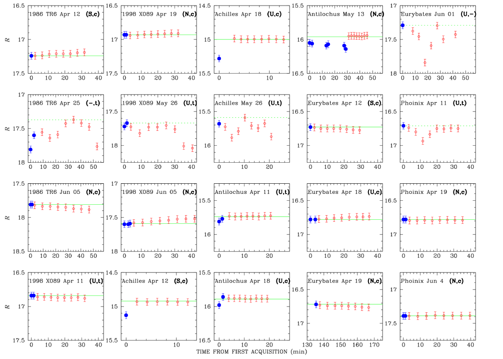
Figure 11: Photometric measurements. The blue solid circles represent the photometry measured in the acquisition images, and the red empty circles represent the photometry measured from the polarimetric images. The green lines show the final value adopted for the time series (dotted green line represent an upper limit). In each panel, between parenthesis we report the ESO QC1 classification of the night (U=unknown, N=non stable, S=stable) followed by the sky conditions as we estimate after inspection of the LOSSAM plots available (c=clear,t=thin to thick). The LOSSAM archive is available online through the ESO website. This Figure is discussed in Sect. 2.3.

FORS acquisition images have a hard-coded $2\times 2$ pixel readout mode. Aperture photometry was calculated on apertures up to 15 pixel, and background was calculated in an annulus with inner radius of 20 and 30 pixels, respectively (corresponding to 5″ and 7.5″). The results of our photometric measurements are also reported in Table 1, and Fig. 11 shows the magnitude measured in each observing series.

2.4 Searching for coma activity

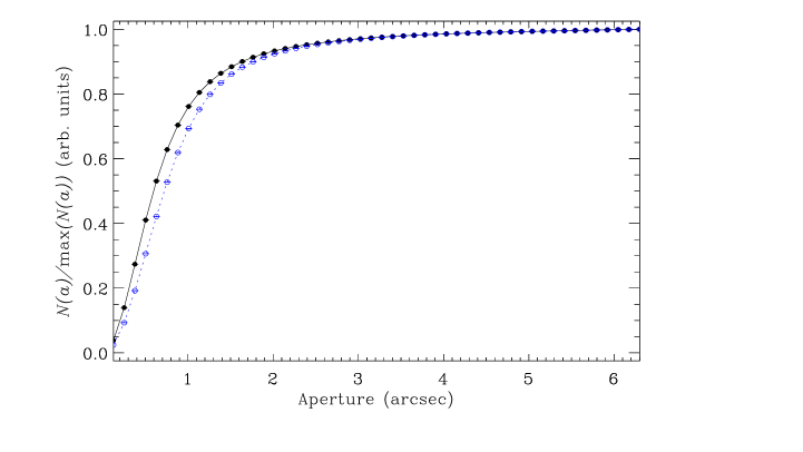
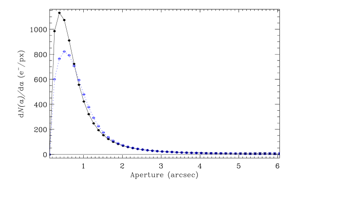
Figure 3: Flux (top panel) and its derivative (bottom panel) as a function of the aperture for asteroid (6545) 1986 TR6 observed on 2013-06-05 (black solid circles and solid lines) and for a background star of similar brightness (blue empty circules and dashed lines).

After background subtraction, all polarimetric frames of each observing series were coadded (combining together both images split by the Wollaston prism and obtained at different positions of the retarder waveplate). The resulting frames were analysed as explained in Sect. 3.2 of Bagnulo et al. (2010) to check for the presence of coma activity. Briefly, we assumed that the number of detected electrons e^- of the object per unit of time within a circular aperture of radius $a$ is the sum of the contribution of the nucleus plus the potential contribution of a coma, plus, possibly, a spurious contribution due to imperfect background subtraction. To check for the presence of a coma, it is probably sufficient to compare the point-spread function (PSF) of the main target with those of the background stars. However, if we are interested in a more quantitative estimate (e.g. an upper limit), following A’Hearn et al. (1984), we can assume that the flux of a weak coma around the nucleus in a certain wavelength band can be written as

$$F_{\mathrm{C}}=Af\left(\frac{\rho}{2r\Delta}\right)^{2}{F_{\odot}}\;,$$ (4)

where $A$ is the bond albedo (unitless), $f$ the filling factor (unitless), $r$ the heliocentric distance expressed in au, $\Delta$ the geocentric distance and $\rho$ the projected distance from the nucleus (corresponding to the aperture). Finally, $F_{\odot}$ is the solar flux at 1 au, integrated in the same band as $F_{\mathrm{C}}$, and convolved with the filter transmission curve. Following the approach of Tozzi & Licandro (2002), Bagnulo et al. (2010) have shown that if the derivative of the flux with respect to the aperture converges to a constant value $k^{\mathrm{(C)}}$, then

$$Af\rho=1.234\,10^{19}\ 10^{0.4\,(m_{\odot}-{ZP}_{m})}\ r^{2}\ \left(\frac{\Delta}{d_{\rm p}}\right)\ k^{\mathrm{(C)}},$$ (5)

where $m_{\odot}$ is the apparent magnitude of the Sun (i.e., at 1 au) in the considered filter, $ZP_{m}$ is the zero point in that filter for the observing night, and $d_{\rm p}$ the CCD pixel scale in arcsec (0.125″ in our case). In Eq. (5) $r$ and $\Delta$ are measured in au and $k^{\mathrm{(C)}}$ in e^- per pixel, and $Af\rho$ is obtained in cm. We found that in all cases, $Af\rho$ is consistent with zero within a typical error bar of $\sim 10$ cm (see Fig. 3). We conclude that there is no evidence of any coma activity.

3 Discussion

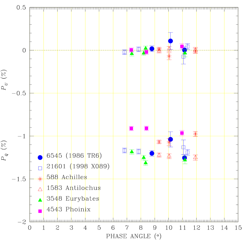
Figure 4: Polarimetric measurements of six Jupiter Trojans asteroids.

All our polarimetric and photometric measurements are reported in Table 1. In the following we first discuss the differences found among our sample, searching for a correlation between polarimetric properties and other characteristics of our objects, then we consider Trojans as a homogeneous class to compare with other atmosphere-less objects of the solar system.

Orbital constraints meant that all six Trojans asteroids were observed in the negative branch, i.e. at those phase angles where we expect that the polarization of the reflected light is parallel to the scattering plane. We measured polarization values from $-1.3$ % to $-0.9$ % in a phase-angle range $7-12\degr$. The variations in polarization within the observed phase-angle range are small for all objects, yet, thanks to the high S/N of our observations, it is possible to distinguish some different behaviours. Figure 4 shows the results of our polarimetric observations as a function of the phase angle.

Several functions have been proposed to fit polarimetric measurements versus phase angle. One of the most popular ones is the one proposed by Lumme & Muinonen (1993):

$$P(\alpha)=b\sin^{c_{1}}(\alpha)\,\cos^{c_{2}}\left(\frac{\alpha}{2}\right)\,\sin(\alpha-\alpha_{0})$$ (6)

where $b$ is a parameter in the range $[0,1]$, $\alpha_{0}$ is the inversion angle (typically $\la 30\degr$), and $c_{1}$ and $c_{2}$ are positive constants. Equation (6) was used, for example, by Penttilä et al. (2005) for a statistical study of the asteroids and comets. The number of our data points per object is even smaller than the number of free parameters, therefore it does not make sense to fit our data without making assumptions (such as about the inversion angle of the polarimetric curves). However, assuming that the minimum of the polarization is reached in the phase-angle range 6°-12° (a typical range for low-albedo objects would be 8°-10°), even a simple visual inspection allow us to estimate the polarization minima of the various objects and, in particular, to conclude that our sample does not show homogeneous polarimetric behaviour.

The object (3548) Eurybates is the largest member of a dynamical family mainly consisting of C-type objects (Fornasier et al. 2007). It has the deepest minimum ($P_{\rm min}\sim-1.3$ %). All the remaining objects belong to the D-type taxonomic class (Grav et al. 2012). The objects (588) Achilles and (4543) Phoinix exhibit a shallower polarization curve (i.e., lower absolute values of the polarization) than the other four Trojans. Figure 4 also suggests that the minimum of the polarization curve of (588) Achilles is reached at a phase-angle value that is lower than that of (4543) Phoinix. Objects (1583) Antilochus, (6545) 1986 TR6, and (21601) 1998 X089 all seem to have similar polarimetric behaviour, with a minimum $\sim-1.2$ %.

Before progressing in our analysis, it is important to discuss whether the observed diversities are real. This question arises since our photon-error bars are very small (a few units in $10^{-4}$), and compared to them, instrumental or systematic errors may not be negligible. However, the relatively smooth behaviour with phase angle and the good consistency with zero of both the $P_{U}$ and the null parameters suggest that our photon-noise error bars are probably representative of the real error. Exceptions to the smooth behaviour are represented by the point at phase angle 10.1°of asteroid (6545) 1986 TR6 (obtained on April 25 2013) and the point at phase angle 8.4° of asteroid (3548) Eurybates (obtained on April 19 2013). Figures 9 and 10 show that, in the former case, polarimetric measurements depend strongly on the aperture and fail to converge to a well-defined value, probably due to the strong background, therefore the observed discrepancy (still within the error bar) is due to a larger error than what is typical in our dataset. The case of asteroid (3548) Eurybates is more puzzling. There is nothing in Fig. 9 that suggests a problem with aperture polarimetry in any of the observations, therefore one may hypothesize that the abrupt change observed between the point at phase 8.1° and the point at phase angle 8.4° is due to asteroid rotation.

The rotation periods of the observed Trojans range from 7.306 h for (588) Achilles to 38.866 h (4543) Phoinix, and their ligtcurves amplitudes are $\la 0.3$ mag. While during an observing series we do not expect short-term photometric variations caused by asteroid rotation, it is possible that polarimetric data depend on the rotation phase at which observations were obtained.

Polarimetric behaviour may depend on the rotational phase of the observations. Although rarely observed, one notable example is that of asteroid (4) Vesta, with a rotational polarimetric amplitude of $\sim 0.03$ % (Wiktorowicz & Nofi 2015) to 0.1 % (Lupishko et al. 1988). To test whether our polarimetric data are rotationally modulated, we calculated the rotation phase shift between observations of each object and found, for instance, that a large shift (0.36) occurs between the observations at phase angles 6.8° and 7.8° of asteroid (21601) (1998 X089). However, the polarization values at these phase angles are consistent with each other, and overall, the polarization curve is relatively smooth. By contrast, the rotation phase shift between phase angles 8.2°and 8.4° of asteroid (3548) Eurybates is only 0.1 of a rotation period. These differences may, therefore, not be due to rotation but instead to photon noise fluctuations or to small changes in the (already small) instrumental polarization. We conclude that there is no obvious evidence of a polarimetric modulation introduced by asteroid rotation in our data. On the other hand, our sample shows a polarimetric behaviour that is not perfectly homogeneous, which must reflect some difference in their surface structure and/or albedo.

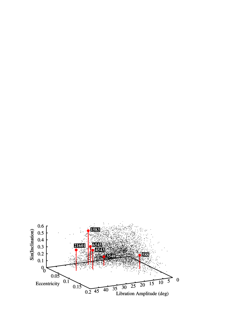
Figure 5: Proper orbital elements of 5020 numbered and multi-opposition Trojans appearing in the database by Knezevic & Milani (last updated in June 2014; available at http://hamilton.dm.unipi.it/$\sim$astdys2/propsynth/tro.syn). The six Trojans observed in this work are indicated by the red points and identified by number.

3.1 Searching for correlation with dynamical and surface properties

3.1.1 Proper orbital elements

No strong correlations have been identified yet between the physical and orbital properties of Trojans, although there appears to be a bimodality in spectral slopes (Szabó et al. 2007; Roig et al. 2008). In confirming a similar bimodality within a sample of near-IR spectra of Trojans, Emery et al. (2011) point out a possible weak correlation with inclination amongst their less-red population. We have searched for trends between polarimetric behaviour and orbital properties in our sample. Figure 5 shows the proper orbital elements of Jupiter Trojans with the six objects observed in this work denoted by red points and identified by their number. All the objects, except (588) Achilles, have low ($\lesssim 0.05$) proper eccentricity and high ($>15^{\circ}$) libration amplitude. We note that the two objects with a shallow polarization curve – (588) Achilles and (4543) Phoinix – also have the highest proper eccentricity in our sample. However, since the eccentricity of (4543) Phoinix ($0.059$) is only marginally higher than those of (3548) Eurybates and 21601 (1998 X089) ($0.044$ and $0.053$, respectively), and given the small size of our sample, we do not attach any high statistical significance to this observation. Finally, there appears to be no trend linking polarization behaviour with inclination; both (588) Achilles and (4543) Phoinix have inclinations within 1 $\sigma$ of the mean for the four other objects.

Table 2: Some parameters of the observed Jupiter Trojans.

			DIAMETER				$H_{V}(\alpha=0\degr)$			ALBEDO ESTIMATES
		$P_{\rm min}$	WISE		AKARI				this					$D_{\rm WISE}\ +$	$D_{\rm AKARI}\ +$
Object	Type	(%)	(km)		(km)		WISE	AKARI	work	WISE		AKARI		$H_{\rm this\ work}$	$H_{\rm this\ work}$
1	2	3	4		5		6	7	8	9		10		11	12
588	DU	$-1.10$	130.1$\pm$	0.6	133.2$\pm$	3.3	8.47	8.67	8.45	0.043$\pm$	0.006	0.035$\pm$	0.002	0.044	0.042
1583	D	$-1.25$	108.8$\pm$	0.5	111.7$\pm$	3.9	8.60	8.60	8.97	0.054$\pm$	0.004	0.053$\pm$	0.004	0.039	0.037
3548	C	$-1.35$	63.9$\pm$	0.3	68.4$\pm$	3.9	9.80	9.50	9.79	0.052$\pm$	0.007	0.060$\pm$	0.007	0.053	0.046
4543	D	$-0.95$	63.8$\pm$	0.4	69.5$\pm$	2.2	9.70	9.70	10.06	0.057$\pm$	0.017	0.049$\pm$	0.003	0.041	0.035
6545	D	$-1.25$	51.0$\pm$	0.6			10.00		10.64	0.068$\pm$	0.009			0.038
21601	D*	$-1.20$	54.9$\pm$	0.4	56.1$\pm$	1.9	9.90	9.40	10.41	0.064$\pm$	0.012	0.100$\pm$	0.007	0.040	0.039

3.1.2 Albedo

It is well known that the minimum of the polarization is inversely correlated to the albedo; i.e., the higher the absolute value of the minimum, the lower the albedo (e.g. Zellner et al. 1977a; Cellino et al. 2015). In fact, various authors have tried to calibrate a relationship

$$\log p=C_{1}\log P_{\rm min}+C_{2}$$ (7)

to estimate the albedo $p$ from polarimetric observations. For instance, Lupishko & Mohamed (1996) give $C_{1}=-1.22$ and $C_{2}=-0.92$; Cellino et al. (2015) give $C_{1}=-1.426\pm 0.034$ and $C_{2}=-0.917\pm 0.006$.

However, it is known that Eq. (7) is only an approximation that does not necessarily produce accurate albedo estimates (e.g. Cellino et al. 2015). In particular, a saturation effect may occur for the darkest objects, which was discovered in the laboratory for very dark surfaces (Zellner et al. 1977b; Shkuratov et al. 1992): the depth of negative polarization increases as the albedo decreases down to $\sim 0.05$, but a further decrease of the albedo results in a decrease in the absolute value of the polarization minimum. This effect was observed for the very dark F-type asteroids by Belskaya et al. (2005) (see also Cellino et al. 2015). In the case of the observed Trojans, the albedo estimated from Eq. (7) and from our polarimetric minima are of the order of 0.08–0.12, which is inconsistent with what has been found from independent estimates of the albedo. We conclude that the polarimetric measurements of our Trojans are also in the regime of ‘saturation’ similar to what was observed for F-type asteroids.

In fact, the albedo estimates from the WISE (Grav et al. 2012) and AKARI (Usui et al. 2011) mid-IR surveys lead to contradictory conclusions. For instance, according to AKARI data (Col. 10 of Table 2), (588) Achilles and (4543) Phoinix (that show the shallower polarization minima) are actually the darkest objects. This finding is somehow contradicted by the WISE albedos (Col. 9), according to which (588) Achilles would still be the darkest object in our sample, but (4543) Phoinix would have an albedo higher than that of (1583) Antilochous and (3548) Eurybates. Albedo estimates strongly depend on the values of absolute magnitudes adopted in the surveys (see Cols. 6 and 7). It is therefore of some interest to recalculate them using our photometric measurements in Table 1.

To calculate the absolute magnitudes, we need to know magnitude-phase dependences of our targets. Shevchenko et al. (2012) have shown that D-type Trojans are characterized by a linear magnitude-phase dependence down to small phase angles without the opposition effect, i.e., that a linear fit gives a more precise estimate of the absolute magnitudes of the D- and P-type Trojans compared to what can be estimated with the so-called HG function (Slyusarev et al. 2012). For the D-type asteroids, we therefore performed a linear extrapolation to zero phase angle assuming a 0.04 mag/deg slope, which is typical of these objects. For the C-type (3548) Eurybates, we assumed a non-linear magnitude-phase dependence similar to that of C-type asteroids (Belskaya & Shevchenko 2000). To calculate the absolute magnitudes $H$ in the $V$ band, we adopted the literature $V-R$ colours of these objects, when available, or assumed $V-R=0.45$ (see Fornasier et al. 2007). Our estimates of the absolute magnitudes $H$ are shown in Col. 8 of Table 2. Although our photometric measurements agree with the measurements of Cols. 6 and 7, they exhibit a systematic negative offset, which may be consistent with the findings by Pravec et al. (2012) of a systematic bias in the absolute magnitudes of asteroids given in the orbital catalogues. Using our revised absolute magnitudes and diameters from WISE and AKARI surveys, we calculated the albedos of our objects again. Our new albedo estimates (Cols. 11 and 12 of Table 2) are no longer as scattered as the original estimates from Usui et al. (2011) and Grav et al. (2012), but actually very similar for all five D-type Trojans.

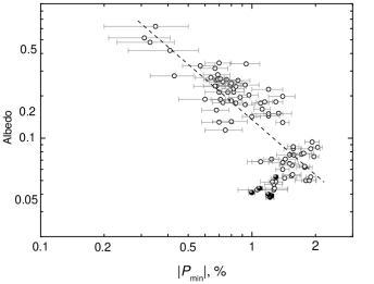
Figure 6: Relationship between albedo and polarization minimum $P_{\rm min}$ for asteroids (open symbols) and Trojans (filled symbols).

The relationship of $P_{\rm min}$ and albedo based on the updated data on albedos is plotted in Fig. 6. Data for Trojans are within the range of the low albedo asteroids. The saturation effect for low-albedo asteroids is fairly evident.

If our new estimates of the albedos are correct, then the differences observed between (4543) Phoinix, (588) Achilles, and the group of three asteroids (1583) Antilochus, (6545) 1986 TR6, and (21601) (1998 X089) may just reflect a difference in the surface structure that could also be revealed, e.g., by a difference in the reflectance spectra. The spectral properties of (4543) Phoinix have not been measured, and (588) Achilles is classified as an unusual D type (DU) by Tholen (1989). The remaining three asteroids are D type. We therefore expect that the taxonomic class of (4543) Phoinix may also differ from the typical D type.

3.2 Comparison with other atmosphere-less objects in the solar system

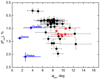
Figure 7: Depth of the polarization minimum $P_{\rm min}$ versus the phase-angle $\alpha_{\rm min}$ where the minimum occurs for asteroids (black) , Trojans (red), and Centaurs (blue points).

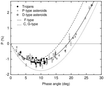
Figure 8: Polarization phase angle dependence of Jupiter Trojans (filled circles), D-type asteroids (open circles), and P-type asteroids (crosses). The fits by a Lumme & Muinonen function are shown for the F-type (dashed line), P-type (solid line), and C,G type (dotted line) asteroids.

We have compared the polarimetric properties of Trojans to the literature data on TNOs (Bagnulo et al. 2008, and references therein), Centaurs (Belskaya et al. 2010, and references therein), and low-albedo asteroids (see database compiled by Lupishko and available at http://sbn.psi.edu/pds/resource/apd.html). The mean values of the polarimetric parameters $P_{\rm min}$, $\alpha_{\rm min}$, $\alpha_{\rm inv}$ and their scattering are given in Table 3.

The polarimetric properties of TNOs and Centaurs are not characterized as well as those of main-belt asteroids. Because of their distance, Centaurs can only be observed in a limited phase angle range ($\sim 0-5\degr$, compared to $\sim 0-30\degr$ of main-belt objects). However, there are indications that the polarimetric curves of Centaurs reach a minimum at very small phase angles (as small as $\sim 1.5\degr$ for Centaur Chiron, see Bagnulo et al. 2006; Belskaya et al. 2010). This feature was interpreted by Belskaya et al. (2010) as indicative of a thin frost layer of submicron water ice crystals on their dark surfaces. Both for Trojans and Centaurs, we can only estimate a lower limit of the inversion angles, since geometrical constraints make their direct measurements impossible from Earth-based observations. For TNOs, that with the exception of the binary system Pluto-Charon are visible from Earth only at phase angles $\la 2$°, we cannot even estimate the parameters $P_{\rm min}$ and $\alpha_{\rm min}$.

Figure 7 shows the relationship of polarization minimum and the phase angle where the minimum occurs for Trojans, Centaurs, and main-belt asteroids. The polarization-phase angle behaviour of the observed Trojans is very similar to that of low-albedo asteroids, in particular the P-type asteroids, and quite different from those Centaurs for which polarimetric measurements have been obtained, in spite of closer proximity to the latter group of objects.

Table 3: Polarimetric properties of some atmosphere-less objects. The number of objects for which polarization minima ($P_{\rm min}$ at $\alpha_{\rm min}$) and inversion angles ($\alpha_{\rm min}$) were measured is indicated by $N_{\rm min}$ and $N_{\rm inv}$, respectively.

		$P_{\rm min}$		$\alpha_{\rm min}$			$\alpha_{\rm inv}$
Object	$N_{\rm min}$	(%)		$(\degr)$		$N_{\rm inv}$	$(\degr)$
Trojans	5	$-1.15$$\pm$	0.15	9$\pm$	1	0	$\ga 17$
P-type	11	$-1.29$$\pm$	0.22	8$\pm$	2	4	19.2$\pm$	1.0
F-type)	4	$-1.17$$\pm$	0.11	7$\pm$	2	4	16.1$\pm$	1.4
G- and C-type	20	$-1.70$$\pm$	0.20	9$\pm$	2	9	20.8$\pm$	0.6
Centaurs	4	$-1.44$$\pm$	0.47	$\sim 2$?		0	$\ga 6$
Small TNOs	0	$<-1.5$		¿2		0	?

Figure 8 shows the mean polarization-phase curves for the P-, F-, G- and C-type asteroids, and demonstrates that the data for the P-type asteroids and D-type Trojans are practically indistinguishable. Compared to the F-type asteroids, polarization minima of Trojans occur at a larger phase-angle, which suggests that their inversion phase-angles are also larger. Fornasier et al. (2006) obtained a polarimetric measurements of the D-type object (944) Hidalgo at a large phase angle, and (944) Hidalgo has an unusual orbit with a semi-major axis of 5.74 au and eccentricity of 0.66. This object reaches 1.94 au in perihelion, giving an opportunity to observe it in much larger phase-angle range than for other D types. The polarization measurement at $\alpha=26.8\degr$ lies exactly at the fitted phase curve for P-type asteroids and confirms a similarity of polarization properties of D- and P-type asteroids within the accuracy of polarimetric measurements.

4 Conclusions

We performed a pilot study of the polarization properties of Jupiter Trojan asteroids and have obtained measurements for six objects belonging to the L4 population. Comparing our targets, we found that they show similar but not identical polarization properties, in particular that there are at least two distinct polarimetric behaviours. Trojans (588) Achilles and (1583) Antilochus show a shallower polarization curve than the remaining four Trojans (3548) Eurybates, (4543) Phoinix, (6545) (1998 TR6), and (21601 (1998 X089). The C-type Trojan (3548) Eurybates shows the deepest minimum of polarization. D-type Trojans (1583) Antilochous, (6545) (1998 TR6) and (21601) (1998 X089) all have a minimum around $-1.2$ %, but overall their polarimetric behaviour does not appear very different from that of (3548) Eurybates. Considering all objects together, we found that the minimum of the polarization is reached at a phase angle $\sim 10\degr$ and is in the range of$-1.3$ % to $-1.0$ %. This polarimetric behaviour is different from that of Centaurs, which seem to show polarization minima at much smaller phase angles and are very similar to low-albedo main-belt asteroids.