Origin of fermion masses without spontaneous symmetry breaking
Abstract
Using a simple three dimensional lattice four-fermion model we argue that massless fermions can become massive due to interactions without the need for any spontaneous symmetry breaking. Using large scale Monte Carlo calculations within our model, we show that this non-traditional mass generation mechanism occurs at a second order quantum critical point that separates phases with the same symmetries. Universality then suggests that the new origin for the fermion mass should be of wide interest.
pacs:
71.10.Fd,02.70.Ss,11.30.Rd,05.30.RtThe origin of mass in the universe is an interesting problem in fundamental physics Wilczek (2012). In continuum quantum field theory, fermion masses arise from local fermion bilinear mass terms that are introduced as parameters in the theory. If symmetries of the theory prevent such terms, perturbatively fermions remain massless. However, these symmetries can break spontaneously and form non-zero fermion bilinear condensates dynamically that can make fermions massive. This well-known mechanism of mass generation is used in the standard model of particle physics to give quarks and leptons their masses. Recent progress in the field of topological insulators suggests the existence of an alternate mechanism for the origin of the fermion mass Kitaev (2009); Fidkowski et al. (2013); Gu and Wen (2014); Metlitski et al. (2014). These studies show that fermions can become massive without spontaneous symmetry breaking due to an interplay of quantum entanglement and topology. In particular, fermion bilinear condensates are not necessary. An example of how the mechanism works in two space-time dimensions has been discussed recently BenTov (2015). Since this alternate mechanism also constrains the number of fermion species of the theory, some speculations that it may explain the particle spectrum of the standard model have also been proposed Wen (2013); You et al. (2014); You and Xu (2015).
Quantum entaglement and topology can be important in determining the ground state properties of matter Chen et al. (2013). They can also lead to exotic second order phase transitions that are characterized by a change in some topological order of the ground state, unlike standard transitions which occur due to spontaneous symmetry breaking characterized by a change in some local order parameter. In certain cases, fractionalization of the fundamental degrees of freedom can occur leading to emergent gauge fields Senthil et al. (2004). Understanding these exotic second order phase transitions is an active area of research today Isakov et al. (2012); Swingle and Senthil (2012). It was recently proposed that the origin of fermion mass without spontaneous symmetry breaking can also be related to a similar exotic quantum phase transition. Evidence for this conjecture was provided using Monte Carlo calculations on small lattices in a model inspired by the physics of electrons hopping on a honeycomb lattice Slagle et al. (2015); He et al. (2015). In this work we show a similar phenomenon in a simple lattice field theory model in three space-time dimensions in the action formalism that is much closer in spirit to particle physics. Due to the simplicity of the model we are able to perform calculations on a much larger scale and estimate the critical exponents. Some of the technical details of our work on small lattices have already appeared earlier in Ayyar and Chandrasekharan (2015) and have also been verified recently in Catterall (2015).
It is possible to understand the alternative mechanism of fermion mass generation qualitatively using four-fermion models. Consider free massless fermions interacting through a four-fermion coupling that has symmetries which forbid the generation of fermion bilinear mass terms through radiative corrections. Since perturbatively four-fermion couplings are irrelevant, the model will contain a massless fermion phase at weak couplings. However at strong couplings such models can be in a massive phase. Traditionally this massive phase is accompanied with spontaneous symmetry breaking and the generation of fermion bilinear condensates. In fact gauge anomalies force the existence of such a phase due to t’Hoofts anomaly matching arguments ’t Hooft (1980). But, if the four-fermion couplings explicitly break all anomalous symmetries while still forbidding fermion bilinear condensates, then there may be a way to circumvent anomaly matching arguments and allow a massive fermion phase without any spontaneous symmetry breaking.
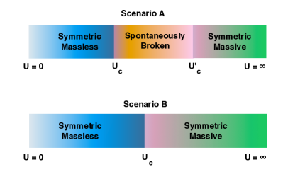
Lattice models that realize the above speculative scenario concretely were constructed and studied long ago Hasenfratz and Neuhaus (1989); Hasenfratz et al. (1990); Lee et al. (1990a, b). These models contained a massless fermion phase at weak couplings and a massive fermion phase at strong couplings. But most interestingly, the massive phase was not accompanied by spontaneous breaking of any symmetries. The two phases were usually separated by a more conventional spontaneously broken phase as shown in Fig. 1 as scenario A. The exotic massive fermion phase without spontaneous symmetry breaking can be interesting in continuum quantum field theory if it is connected to the massless fermion phase directly through a second order transition. This is shown as scenario B in Fig. 1. The presence of a second order critical point will allow one to take the continuum limit of the massive fermion phase and thus eliminate the effects of lattice discretization. Most earlier work had focused on four Euclidean dimensions, and a direct second order transition was never discovered, although some mean field theory calculations predicted a direct first order transition Stephanov and Tsypin (1990a, b). In our work we focus on three Euclidean dimensions and find strong evidence for a direct second order transition (scenario B in Fig. 1).
The model we study contains four flavors of massless reduced lattice staggered fermions on a cubical space-time lattice with an onsite four-fermion interaction. Each lattice fermion flavor describes a single four-component Dirac fermion in the continuum due to fermion doubling Sharatchandra et al. (1981); van den Doel and Smit (1983); Golterman and Smit (1984).Our model can be obtained as a limit of lattice Yukawa models that were studied long ago in four space-time dimensions Lee et al. (1990a, b). Further, our model has the same fermion content as the honeycomb lattice models studied recently Slagle et al. (2015); He et al. (2015). We use four-component Grassmann valued fields, , on each lattice site to describe the fermion fields. Then, the Euclidean action of our model is given by :
| (1) |
where is the well known massless staggered fermion matrix given by
| (2) |
where are phases that introduce a -flux through all plaquettes. In our work we study cubical lattices of equal size in each direction with anti-periodic boundary conditions. Observables are defined as usual through the Grassmann integral
| (3) |
where is the partition function.
The action given in Eq. (1) is symmetric under the usual space-time lattice transformations and an internal flavor transformations Ayyar and Chandrasekharan (2015). Using weak coupling and strong coupling perturbation theory, it is easy to argue that all lattice symmetries remain unbroken at both weak and strong couplings. Thus, the essential question is whether there is a single transition between the two phases or is there an intermediate phase where some of the lattice symmetries are broken. Previous studies in four space-time dimensions do seem to find such an intermediate phase. Here we present clear evidence from large lattices for a single second order transition between the two phases in three space-time dimensions and estimate the critical exponents at the transition.
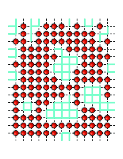
We perform calculations using the fermion bag approach Chandrasekharan (2010) where the problem is converted into a statistical mechanics of monomer configurations which we denote as . Each monomer configuration is defined through a binary lattice field which denotes the absence or presence of a monomer at the site respectively. Figure 2 shows an illustration of a monomer configuration on a two dimensional lattice. Each monomer represents a four-fermion interaction and free fermions hop on sites that do not contain monomers. The fermion bag approach also gives a very intuitive picture of the underlying physics: At small couplings the monomer density is small and fermions are essentially free, while at strong couplings the lattice is filled with monomers with very few empty sites for free fermions to hop making them massive. Since monomers form local singlets, both phases have the same lattice symmetries. Further details of our computational approach, including algorithms that we use can be found in Ayyar and Chandrasekharan (2015).
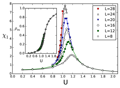
In our earlier work we presented evidence for a single continuous phase transition between the massless and the massive phases up to lattice sizes of . The main result is summarized in Fig. 3 where we plot the monomer density and one of the fermion bilinear susceptibilities , as a function of for various values of . The behavior of these observables is consistent with a single phase transition around . Most importantly, the bilinear susceptibility never increases like showing the absence of any local fermion bilinear condensate for all values of . Recently it was also confirmed that other discrete lattice symmetries, like the shift symmetry, also remain unbroken for all values of Catterall (2015).
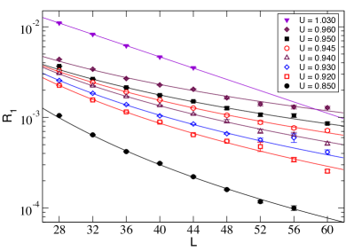
We now have results from much larger lattices (up to ) that further confirm a single second order transition. We can also roughly estimate the critical exponents if we assume the absence of corrections to scaling on lattices above . Here we focus on the two independent bosonic correlation functions and where is varied along the time direction. Near the critical point both these correlation functions are comparable to each other, while vanishes at . For the purpose of comparing different lattice sizes, we extract the correlation ratios and as a function of . For large , these ratios are expected to scale as in the massless phase, as at the critical point and as in the massive phase. Here is one of the standard critical exponents. Our data is consistent with this behavior for . In table 1 we show the combined fit results of our data to the form near the critical region. As an illustration of the goodness of our fits, in Fig. 4 we plot as a function of along with the fits. Based on this we estimate that the critical point is somewhere in the region . For a single power law no longer fits the data well, but an exponential fit begins to work well. For example, a fit to the form at is shown in Fig. 4.
| /DOF | /DOF | ||||
|---|---|---|---|---|---|
| 0.000 | – | 0.850 | 2.5 | ||
| 0.920 | 4.6 | 0.930 | 1.9 | ||
| 0.940 | 1.0 | 0.945 | 0.7 | ||
| 0.950 | 1.1 | 0.960 | 6.4 |
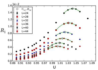
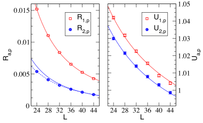
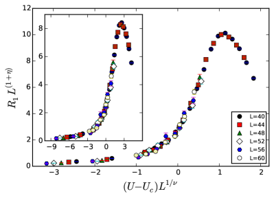
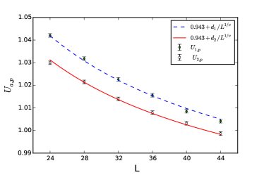
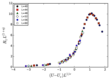
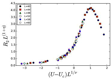
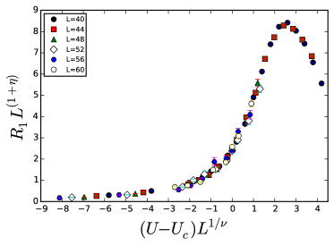
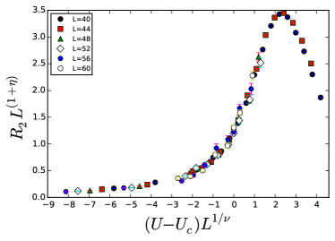
Since it is difficult to locate and compute from the data in the region we have also analyzed a different scaling region of where , show a peak. In Fig. 5 we plot the behavior of the correlation ratio as a function of the coupling for different lattices sizes. A similar plot exists for Sup . Note that the correlation ratios display a maximum as a function of for a fixed . We have computed these maximum values , and their locations , in the range . From scaling theory, we expect and . We find that fits well to this expected form for , while does not. However if we keep only the data from the largest lattices for both and we can again perform combined fits to the expected scaling form without the need for corrections to scaling. Interestingly, allowing a scaling correction only for allows us to fit the entire data set. Two of these fits are shown in the left plot of Fig. 6. Using these fits and including various systematic errors we estimate . Combining this result with that of Table 1, we constrain . Using this result along with our data for and its expected scaling form we can again perform combined fits to obtain . One such fit is shown in the right plot of Fig. 6. Using these fits we estimate . In Fig. 7 we verify if our large lattice data falls on a single universal scaling function when we fix , and . The fact that the data falls on a single curve gives us confidence that this is indeed the case. However, we must note that if we allow for scaling corrections to be present in our fits we cannot rule out , and as expected from large four-fermion models Hands et al. (1993). The universal scaling with these “mean field” parameters is shown in the inset of Fig. 7.
To summarize, we have established the existence of a three dimensional exotic second order phase transition between a massless and a massive fermion phase, both of which have the same lattice symmetries. Thus, fermion mass generation is not necessarily driven by spontaneous symmetry breaking contrary to conventional wisdom.
The material presented here is based upon work supported by the U.S. Department of Energy, Office of Science, Nuclear Physics program under Award Number DE-FG02-05ER41368. An important part of the computations performed in this research was done using resources provided by the Open Science Grid, which is supported by the National Science Foundation and the U.S. Department of Energy’s Office of Science Pordes et al. (2007); Sfiligoi et al. (2009).
References
- Wilczek (2012) F. Wilczek, Central Eur. J. Phys. 10, 1021 (2012), eprint 1206.7114.
- Kitaev (2009) A. Kitaev, AIP Conf.Proc. 1134, 22 (2009), eprint 0901.2686.
- Fidkowski et al. (2013) L. Fidkowski, X. Chen, and A. Vishwanath, Phys.Rev. X3, 041016 (2013), eprint 1305.5851.
- Gu and Wen (2014) Z.-C. Gu and X.-G. Wen, Phys. Rev. B90, 115141 (2014), eprint 1201.2648.
- Metlitski et al. (2014) M. A. Metlitski, L. Fidkowski, X. Chen, and A. Vishwanath (2014), eprint 1406.3032.
- BenTov (2015) Y. BenTov, JHEP 07, 034 (2015), eprint 1412.0154.
- Wen (2013) X.-G. Wen, Chin.Phys.Lett. 30, 111101 (2013), eprint 1305.1045.
- You et al. (2014) Y. You, Y. BenTov, and C. Xu (2014), eprint 1402.4151.
- You and Xu (2015) Y.-Z. You and C. Xu, Phys.Rev. B91, 125147 (2015), eprint 1412.4784.
- Chen et al. (2013) X. Chen, Z.-C. Gu, Z.-X. Liu, and X.-G. Wen, Phys. Rev. B87, 155114 (2013), eprint 1106.4772.
- Senthil et al. (2004) T. Senthil, A. Vishwanath, L. Balents, S. Sachdev, and M. P. A. Fisher, Science 303, 1490 (2004).
- Isakov et al. (2012) S. V. Isakov, R. G. Melko, and M. B. Hastings, Science 335, 193 (2012).
- Swingle and Senthil (2012) B. Swingle and T. Senthil, Phys. Rev. B 86, 155131 (2012).
- Slagle et al. (2015) K. Slagle, Y.-Z. You, and C. Xu, Phys. Rev. B91, 115121 (2015), eprint 1409.7401.
- He et al. (2015) Y.-Y. He, H.-Q. Wu, Y.-Z. You, C. Xu, Z. Y. Meng, and Z.-Y. Lu (2015), eprint 1508.06389.
- Ayyar and Chandrasekharan (2015) V. Ayyar and S. Chandrasekharan, Phys. Rev. D91, 065035 (2015), eprint 1410.6474.
- Catterall (2015) S. Catterall (2015), eprint 1510.04153.
- ’t Hooft (1980) G. ’t Hooft, NATO Sci. Ser. B 59, 135 (1980).
- Hasenfratz and Neuhaus (1989) A. Hasenfratz and T. Neuhaus, Phys.Lett. B220, 435 (1989).
- Hasenfratz et al. (1990) A. Hasenfratz, W.-q. Liu, and T. Neuhaus, Phys.Lett. B236, 339 (1990).
- Lee et al. (1990a) I.-H. Lee, J. Shigemitsu, and R. E. Shrock, Nucl.Phys. B334, 265 (1990a).
- Lee et al. (1990b) I.-H. Lee, J. Shigemitsu, and R. E. Shrock, Nucl.Phys. B330, 225 (1990b).
- Stephanov and Tsypin (1990a) M. A. Stephanov and M. Tsypin, Phys.Lett. B236, 344 (1990a).
- Stephanov and Tsypin (1990b) M. A. Stephanov and M. Tsypin, Phys.Lett. B242, 432 (1990b).
- Sharatchandra et al. (1981) H. Sharatchandra, H. Thun, and P. Weisz, Nucl.Phys. B192, 205 (1981).
- van den Doel and Smit (1983) C. van den Doel and J. Smit, Nucl.Phys. B228, 122 (1983).
- Golterman and Smit (1984) M. F. Golterman and J. Smit, Nucl.Phys. B245, 61 (1984).
- Chandrasekharan (2010) S. Chandrasekharan, Phys. Rev. D 82, 025007 (2010).
- (29) See Supplemental Material for further details of the analysis presented.
- Hands et al. (1993) S. Hands, A. Kocic, and J. B. Kogut, Annals Phys. 224, 29 (1993).
- Pordes et al. (2007) R. Pordes et al., J. Phys. Conf. Ser. 78, 012057 (2007).
- Sfiligoi et al. (2009) I. Sfiligoi, D. C. Bradley, B. Holzman, P. Mhashilkar, S. Padhi, and F. Wurthwein, WRI World Congress on Computer Science and Information Engineering 2, 428 (2009).
Supplementary Material
In this supplementary material we explain the analysis used to arrive at the results presented in the main paper.
Observables
The three quantities we focus on in the paper are the monomer density and the two independent correlation functions defined as
| (4) | |||||
| (5) | |||||
| (6) |
The correlation functions are defined between the origin and an arbitrary lattice site that varies along the time direction.
In principle there are six onsite fermion bilinear operators through which we can define different correlation functions. However, due to the symmetry of the model all these correlation functions are related to the above two independent correlation functions. If we consider the origin as an even site, it is easy to argue that for a non-vanishing correlation function, must be an odd site in the case of and it must be an even site in the case of . The monomer density is related to the second correlation function through the relation . Since for small , we can argue that approaches zero at small but not . On the other hand close to the critical point the two correlation functions are very similar and are expected to scale identically with respect to for large values of . In the earlier work we measured the susceptibilty
| (7) |
which turned out to be computationally expensive with our modified algorithm that allows us to explore large lattices. Hence we have focused on the correlation ratios in this work, which are defined as
| (8) | |||||
| (9) |
These ratios help us extract the interesting infrared physics, by removing any multiplicative renormalizations that may arise from the ultraviolet.
I Critical Scaling
The correlation ratios and depend on both (the coupling) and (the lattice size) and near the critical point they are expected to scale according to the form :
| (10) |
where are universal functions of the variable . We use this behavior to extract the critical exponents in our work. For example when we expect
| (11) |
where is a constant and the critical exponent is the same for both and . Interestingly even in the free theory one expects the above form to hold except that . In fact for sufficiently large , we expect in the entire massless phase.
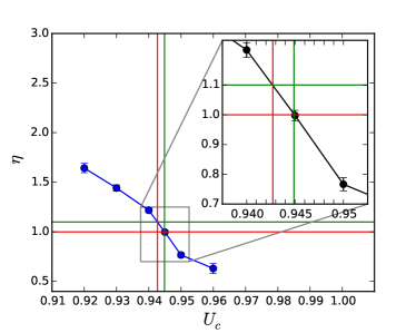
Unfortunately since we do not know the location of the critical point nor the value of at that point, it is difficult to compute and together using the above relation. This is typical of all second order critical points and one usually finds that many couplings near the critical point obey power law scaling with slightly different values of . A combined fit of both correlation ratios to the form given in (11) for the couplings in the range and lattice sizes , yields the results shown in Table 2.
| 0.85 | 68(10) | 38(5) | 2.2 | |
| 0.92 | 15(3) | 8(1) | 4.1 | |
| 0.93 | 9(1) | 4.5(5) | 1.9 | |
| 0.94 | 4.8(4) | 2.4(2) | 1.0 | |
| 0.945 | 2.5(2) | 1.2(1) | 0.7 | |
| 0.95 | 1.2(1) | 0.59(5) | 1.1 | |
| 0.96 | 1.0(2) | 0.46(8) | 6.4 |
Indeed the critical point could be at any value of in the range . The behavior of as a function of is shown in Fig 8. In our analysis we will use an independent procedure to estimate and then use it to constrain along with this figure. Note that for the fit is poor, indicating perhaps that we have reached the massive phase.
II Scaling of Pseudo-Critical Points
While critical points are defined only in the thermodynamic limit, there exists a notion of pseudo-critical points even in a finite system. Interestingly, quantities close to the pseudo-critical points also obey critical scaling and thus can help in the extraction of critical quantities independently. Consider for example the variation of correlation ratios and with coupling at a fixed value of . This is shown in Fig. 9 for different lattice sizes. It is clear from the figure that the ratios display a maximum for certain value of the coupling (which we refer to as ). These define pseudo-critical couplings. At the peak, the value of the ratio itself is given by . From the scaling relation in eqn 10, we note that the peak occurs when the function reaches a maximum. Assuming this occurs at , we can derive
| (12) | |||||
| (13) |
Thus, if we can compute as a function of , we would have an independent way to estimate using (12). As we explained above, we can then use the vs. plot of Fig. (8), in order to estimate . Then using this value of in (13) we can compute . This will be our strategy.

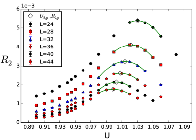
We approximate the behavior of the correlation ratios around the peak as a quadratic to extract and . Table 3 shows our results of such fits. The errors in the fits shown include systematic errors associated with choosing a quadratic form near the peak instead of say a cubic or quartic form.
| /dof | /dof | |||||
|---|---|---|---|---|---|---|
| 24.0 | 0.473 | 1.734 | ||||
| 28.0 | 0.1622 | 0.8016 | ||||
| 32.0 | 1.519 | 1.407 | ||||
| 36.0 | 1.752 | 2.004 | ||||
| 40.0 | 0.4788 | 0.21 | ||||
| 44.0 | 0.7981 | 0.9341 |
II.1 Scaling Fits for
Using the data for and from table 3 we have performed a combined fit of the form expected in (12). Including the entire data from above () gives us , , , . A closer examination shows that while fits well to a single power law in the entire region giving , with a , is not consistent with a single power law. Table 4 shows the results of fitting individually and dropping the lower lattice sizes systematically.
| -Range | /dof | ||
|---|---|---|---|
| 24-44 | 6.3 | ||
| 28-44 | 3.9 | ||
| 32-44 | 2.3 | ||
| 36-44 | 2.2 | ||
| 40-44 | 0.0 |
We interpret the drift of to larger values as a sign that contains pronounced corrections to scaling. If we only keep the lattice sizes of in the data and perform a combined fit of both and we obtain , , , . The goodness of the fit is shown in the left plot of Fig. 10.
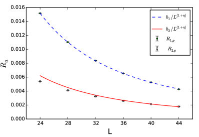
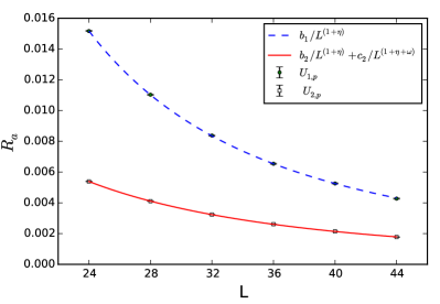
In order to confirm that the drift of is consistent with the presence of corrections to scaling, we added a correction term for and performed a combined fit of the entire data to the form:
| (14) | |||||
| (15) |
Now including the entire data set in table 3, we find a good fit as shown in the right plot of Fig. 10 , giving us , , , , , . This gives some credence to our belief that data contains corrections to scaling.
However, there is a bias in the above analysis since it is likely that the presence of smaller lattice data in affects the fitting. Hence we roughly estimate the systematic errors in due to the the range of lattice sizes we use in the fit. Keping only data for both and and ignoring corrections to scaling we obtained but with a which is rather large. But by keeping and dropping instead we get a good fit but with . Thus, a conservative estimate would be .
II.2 Scaling Fits for
Using we can again conservatively estimate from Fig. 8 to be . We can then use (13) to estimate . Again assuming no corrections to scaling we find that a combined fit of both the data and fits well to single power law. Performing two fits by fixing and we obtain . The goodness of the fits, assuming , are shown in Fig. (11). For this value of we obtain and and the /dof = 1.0.
III Corrections to Scaling
Since we have ignored corrections to scaling in the analysis above, one might wonder if introducing corrections to scaling can change the results. Experience tells us that usually once we include corrections to scaling the fits become unstable unless we can constrain at least some of the exponents by other arguments. This is difficult in our context due to the exotic nature of the phase transition. There is little information to go by. Still we can ask if, for example, our data is consistent with the exponents from large predictions in a typical Gross Neveu model, i.e., and .
Assuming no corrections to scaling, but fixing and removing data for for which gave a good fit above yields , , with a /dof= 21. The fit is shown on the left plot of Fig. 12. We note that the fit does seems to roughly pass through all the points although the the /dof is large. The reason for this is that our data is quite precise and we are sensitive to corrections to scaling assuming they are present. Indeed, if we introduce corrections to scaling and assume
| (16) |
and fix for example then one can fit the entire data set () for both correlation ratios very well. We obtain , , , , with a /dof . The goodness of the fit is shown in the right plot of Fig. 12.
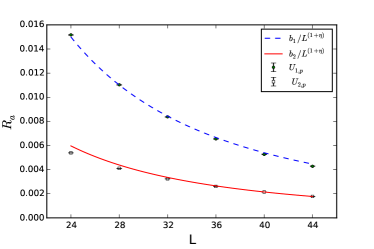
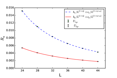
From table 2, we note that gives assuming the corrections to scaling are small at the critical point. Fixing and , a combined fit of and data to the form (13) gives , with a /dof . This is clearly a bad fit as shown in the left plot of Fig. 13. On the other hand if we introduce corrections to scaling and assume
| (17) |
with , and as before, we obtain a good fit as shown in the right plot of Fig 13. The fit yields , , , which a /dof . If we do not fix while ignoring the corrections to scaling, again we obtain a good fit with , , , and /dof . However, this value of cannot be consistent with our data in table 2, again suggesting the presence of large corrections to scaling.
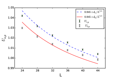
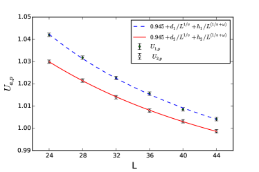
Thus, we believe that including scaling corrections will enable us to fit the data to large exponents of and . However, if we take this view point one has to argue that there are significant corrections to scaling even up to . On the other hand since we were able to fit the data without corrections to scaling to a different set of exponents, it is likely that our original analysis may in fact be correct.
IV Universal Function
In order to contrast the analysis that ignored corrections to scaling and that which included the corrections to scaling but fixed and to their large values, we plot the universal function introduced in (10). For this purpose we plot as a function of . The plot using , and is shown in Fig. 14, while the plot using , and is shown in in Fig. 15. To the eye both curves look reasonable, although as explained above significant corrections to scaling are required before the data can be fit to the latter exponents.
Based on the above analysis we can conclude that either we have a new set of exponents with and , or there are large corrections to scaling up to lattice sizes of the order of and the exponents are very close to the large values.
While calculations at larger lattice may be useful to get better estimates of the critical exponents, given the difficulty in performing large scale Monte Carlo calculations it will be useful to explore a new technique of analysis that reduces the systematic errors due to corrections to scaling.