Optimal Error Estimates for Semidiscrete Galerkin approximations to the Equations of Motion Described by Kelvin-Voigt Viscoelastic Fluid Flow Model

Abstract

In this paper, the finite element Galerkin method is applied to the equations of motion arising in the Kelvin-Voigt viscoelastic fluid flow model, when the forcing function is in $L^{\infty}({\bf L}^{2})$. Some a priori estimates for the exact solution, which are valid uniformly in time as $t\mapsto\infty$ and even uniformly in the retardation time $\kappa$ an $\kappa\mapsto 0,$ are derived. It is shown that the semidiscrete method admits a global attractor. Further, with the help of a priori bounds and Sobolev-Stokes projection, optimal error estimates for the velocity in $L^{\infty}(\bf{L}^{2})$ and $L^{\infty}({\bf{H}}^{1})$-norms and for the pressure in $L^{\infty}(L^{2})$-norm are established. Since the constants involved in error estimates have an exponential growth in time, therefore, in the last part of the article, under certain uniqueness condition, the error bounds are established which are valid uniformly in time. Finally, some numerical experiments are conducted which confirm our theoretical findings.

Keywords: Kelvin-Voigt viscoelastic model, a priori bounds, global attractor, semidiscrete Galerkin approximations, optimal error estimates, uniqueness condition.
AMS 1991 Classification:

1 Introduction

Consider the following system of partial differential equations arising in the Kelvin-Voigt’s model

$$\frac{\partial{\bf u}}{\partial t}+{\bf u}\cdot\nabla{\bf u}-\kappa\Delta{\bf u}_{t}-\nu\Delta{\bf u}+\nabla p={\bf{f}}(x,t),\,\,\,x\in\Omega,\,\,t>0,$$ (1.1)

and incompressibility condition

$$\nabla\cdot{\bf u}=0,\,\,\,x\in\Omega,\,t>0,$$ (1.2)

with initial and boundary conditions

$${\bf u}(x,0)={\bf u}_{0}\;\;\;\mbox{in}\;\Omega,\;\;\;\;\;{\bf u}=0,\;\;\;\mbox{on}\;\partial\Omega,\;t\geq 0,$$ (1.3)

where, $\Omega$ is a bounded convex polygonal or polyhedral domain in ${{\rm I{\!}\rm R}}^{d},d=2,3$ with boundary $\partial\Omega.$ Here, $\nu$ is the coefficient of kinematic viscosity and $\kappa$ is the retardation time or the time of relaxation of deformations. In the context of viscoelastic fluid, this model was first introduced by Pavlovskii [16], who called it as a model describing the motion of weakly concentrated water-polymer solutions. It was called Kelvin-Voigt model by Oskolkov [20] and his collaborators. Subsequently, Cao et. al. [6] proposed it as a smooth, inviscid regularization of the 2D and 3D-Navier-Stokes equations. For applications of such models in organic polymer and food industry, and in the mechanisms of diffuse axonal injury, etc., we refer to [4], [5] and [7].

Earlier, based on the analysis of Ladyzenskaya [15] in the context of Navier Stokes equations, Oskolkov [21]-[22] have proved existence of a unique ‘almost’ classical solution in finite time interval for the problem (1.1)-(1.3). Subsequently, further investigations on solvability were continued by group members of Oskolkov, see [24] and [25].

On numerical analysis of such problems, Oskolkov et a. [23] have discussed the convergence analysis of the spectral Galerkin approximation for all $t\geq 0$ assuming that the exact solution is asymptotically stable as $t\rightarrow\infty.$ Subsequently, Pani et a. [17] have applied a variant of nonlinear semidiscrete spectral Galerkin method and optimal error estimates are proved. It is, further, shown that a priori error estimates are valid uniformly in time under uniqueness assumption. Recently, Bajpai et al. [1] have applied finite element Galerkin methods for the problem (1.1)-(1.3) with the forcing function ${\bf{f}}=0.$ They have proved a priori bounds for the exact solution in $3D$ and established exponential decay property. With an introduction of the Sobolev-Stokes projection, they have derived optimal error estimates, which again preserve the exponential decay property. In [2], completely discrete schemes which are based on both backward Euler and second order backward difference methods are analyzed and optimal error bounds which again preserve exponential decay property are established. For related articles in the context of Oldroyd viscoelastic model, we refer to [10]-[12], [18, 19], [26]-[29].

In this paper, we, further, continue the investigation on finite element approximation to the problem (1.1)-(1.3) when the non-zero forcing function ${\bf{f}}$ belongs to $L^{\infty}(\bf{L}^{2}).$ This is crucial particularly in the study of the dynamical system (1.1)-(1.3), when the forcing function is assumed to be time independent. The major results obtained in this paper are summarized as follows:

• New regularity results for the solution of (1.1)-(1.3) even in $3D$, which are valid uniformly in time are derived and as a consequence, existence of a global attractor is proved. It is further shown that these estimates hold uniformly in $\kappa$ as $\kappa\mapsto 0.$

• When ${\bf{f}}$ is independent of time, it is, further, established that the semi-discrete finite element method admits a discrete global attractor.

• Based on the Sobolev-Stokes projection introduced earlier in [1], optimal error estimates for the semidiscrete Galerkin approximations to the velocity in $L^{\infty}({\bf L}^{2})$-norm as well as in $L^{\infty}({\bf H}^{1}_{0})$-norm and to the pressure in $L^{\infty}(L^{2})$-norm are derived with error bounds depending on exponential in time.

• Moreover, it is proved under uniqueness assumption that error estimates are valid uniformly in time.

Note that for (i), exponential weight functions in time are used which help us to derive regularity result for all $t>0.$ A special care is taken to show that these estimates are valid uniformly in $\kappa$ as $\kappa\mapsto 0.$ When ${\bf{f}}$ is independent of time, based on uniform estimates in time existence of a global attractor is shown for the semidiscrete scheme. For (iii), a use of Sobolev-Stokes projection as an intermediate projection helps us to retrieve optimal error estimates for the velocity vector in $L^{\infty}(\bf{L})$-norm. When either ${\bf{f}}=0$ or ${\bf{f}}=O(e^{-\alpha_{0}t}),$ we derive, as in [1], exponential decay property not only for the solution, but also for error estimates.

This paper is organized as follows. In Section 2, we discuss the weak formulation and state some basic assumptions. Section 3 is devoted to development of a priori bounds for the exact solutions. In Section ${\bf 4}$, we describe the semidiscrete Galerkin approximations and derive a priori estimates with discrete global attractor for the semidiscrete solutions. In Section 5, we establish optimal error estimates for the velocity. Section 6 deals with the optimal error estimates for the pressure. In Section 7, results of numerical experiments, which confirm our theoretical estimates, are established.

2 Preliminaries and Weak formulation

In this section, we define $\mathbb{R}^{d},\;(d=2,3)$-valued function spaces using boldface letters as

$${\bf H}_{0}^{1}=(H_{0}^{1}(\Omega))^{d},\;\;\;{\bf L}^{2}=(L^{2}(\Omega))^{d}\;\;\mbox{and }\;\;{\bf H}^{m}=(H^{m}(\Omega))^{d},$$

where $L^{2}(\Omega)$ is the space of square integrable functions defined in $\Omega$ with inner product $(\phi,\psi)=\displaystyle{\int_{\Omega}}\phi(x)\psi(x)\,dx$ and norm $\|\phi\|=\left(\displaystyle{\int_{\Omega}}|\phi(x)|^{2}\,dx\right)^{1/2}$. Further, $H^{m}(\Omega)$ denotes the standard Hilbert Sobolev space of order $m\in\mathbb{N^{+}}$ with norm $\|\phi\|_{m}=\left(\displaystyle{\sum_{|\alpha|\leq m}}\displaystyle{\int_{\Omega}}|D^{\alpha}\phi|^{2}\,dx\right)^{1/2}$. Note that ${\bf{H}}^{1}_{0}$ is equipped with a norm

$$\|\nabla{\bf v}\|=\left(\displaystyle{\sum_{i,j=1}^{d}}(\partial_{j}v_{i},\partial_{j}v_{i})\right)^{1/2}=\left(\displaystyle{\sum_{i=1}^{d}}(\nabla v_{i},\nabla v_{i})\right)^{1/2}.$$

Further, introduce divergence free spaces :

$${\bf J}_{1}=\{{\mbox{\boldmath$\phi$}}\in{\bf{H}}_{0}^{1}:\nabla\cdot\mbox{\boldmath$\phi$}=0\}$$

and

$${\bf J}=\{\mbox{\boldmath$\phi$}\in{\bf{L}}^{2}:\nabla\cdot\mbox{\boldmath$\phi$}=0\;\;{\mbox{\rm in}}\;\;\Omega,\;\;\mbox{\boldmath$\phi$}\cdot{\bf{n}}|_{\partial\Omega}=0\;\;{\mbox{\rm holds}\;{\rm weakly}}\},$$

where ${\bf{n}}$ is the outward normal to the boundary $\partial\Omega$ and $\mbox{\boldmath$\phi$}\cdot{\bf{n}}|_{\partial\Omega}=0$ should be understood in the sense of trace in ${\bf{H}}^{-1/2}(\partial\Omega)$, see [temam]. Let $H^{m}/{\rm I\!R}$ be the quotient space with norm $\|p\|_{H^{m}/{\rm I\!R}}=\inf_{c\in{\rm I\!R}}\|p+c\|_{m}$. For a Banach Space $X$ with norm $\|\cdot\|_{X},$ let $L^{p}(0,T;X)$ denote the space of measurable $X$- valued functions $\phi$ on $(0,T)$ such that $\int_{0}^{T}\|\mbox{\boldmath$\phi$}(t)\|^{p}_{X}dt<\infty\;\;\;{\mbox{\rm if}}\;\;1\leq p<\infty$ and for $p=\infty$, ${\displaystyle{ess\sup_{0<t<T}}}\|\mbox{\boldmath$\phi$}(t)\|_{X}<\infty.$ Now, set $P:{\bf L}^{2}\longrightarrow{\bf J}$ as the ${\bf L}^{2}$- orthogonal projection.

Throughout this paper, the following assumptions are made.
(A1). Setting $-\tilde{\Delta}=-P\Delta:{\bf J}_{1}\cap{\bf H}^{2}\subset{\bf J}\rightarrow{\bf J}$ as the Stokes operator, assume that the following regularity result holds:

$$\|{\bf v}\|_{2}\leq C\|\tilde{\Delta}{\bf v}\|\;\;\;\;\forall{\bf v}\in{\bf J}_{1}\cap{\bf H}^{2}.$$ (2.1)

The above assumption is valid as the domain $\Omega$ is a convex polygon or convex polyhedron. Note that the following Poincaré inequality [13] holds true:

$$\|{\bf v}\|^{2}\leq\lambda_{1}^{-1}\|\nabla{\bf v}\|^{2}\;\;\forall{\bf v}\in{\bf H}_{0}^{1}(\Omega),$$ (2.2)

where $\lambda_{1}^{-1}$, is the best possible positive constant depending on the domain $\Omega.$ Further, observe that

$$\|\nabla{\bf v}\|^{2}\leq\lambda_{1}^{-1}\|\tilde{\Delta}{\bf v}\|^{2}\;\;\forall{\bf v}\in{\bf J}_{1}\cap{\bf H}^{2}.$$ (2.3)

(A2). There exists a positive constant $M$ such that the initial velocity ${\bf u}_{0}$ and the external force ${\bf{f}},{\bf{f}}_{t}$ satisfy for $t\in(0,\infty)$

$${\bf u}_{0}\in{\bf H}^{2}\cap{\bf J}_{1},\,{\bf{f}},\;{\bf{f}}_{t}\in L^{\infty}(0,\infty;\,\bf{L}^{2})\,\,\rm{with}\,\,\|{\bf u}_{0}\|_{2}\leq M,\,\,\displaystyle{\mathop{ess\,\sup}_{0<t<\infty}}\,\|{\bf{f}}(\cdot,t)\|\leq M.$$

Now, the weak formulation of (1.1)-(1.3) is to seek a pair of functions $({\bf u}(t),p(t))\in{\bf{H}}_{0}^{1}\times L^{2}/{\rm I\!R}$ with ${\bf u}(0)={\bf u}_{0}$, such that for all $t>0$

$$\left.\begin{array}[]{rcl}&&({\bf u}_{t},\mbox{\boldmath$\phi$})+\kappa(\nabla{\bf u}_{t},\nabla\mbox{\boldmath$\phi$})+\nu(\nabla{\bf u},\nabla\mbox{\boldmath$\phi$})+({\bf u}\cdot\nabla{\bf u},\mbox{\boldmath$\phi$})=(p,\nabla\cdot\mbox{\boldmath$\phi$})+(\bf f,\mbox{\boldmath$\phi$})\;\forall\mbox{\boldmath$\phi$}\in{\bf H}_{0}^{1},\\ &&(\nabla\cdot{\bf u},\chi)=0\;\;\;\;\;\;\;\forall\chi\in L^{2}.\end{array}\right\}$$ (2.6)

Equivalently, find ${\bf u}(t)\in{\bf J}_{1}$ with ${\bf u}(0)={\bf u}_{0}$ such that for $t>0$

$$({\bf u}_{t},\mbox{\boldmath$\phi$})+\kappa(\nabla{\bf u}_{t},\nabla\mbox{\boldmath$\phi$})+\nu(\nabla{\bf u},\nabla\mbox{\boldmath$\phi$}) +({\bf u}\cdot\nabla{\bf u},\mbox{\boldmath$\phi$})=(\bf f,\mbox{\boldmath$\phi$})\;\;\;\forall\mbox{\boldmath$\phi$}\in{\bf J}_{1}.$$ (2.7)

Define the trilinear form $b(\cdot,\cdot,\cdot)$ as

$$b({\bf v},{\bf w},\mbox{\boldmath$\phi$}):=\frac{1}{2}({\bf v}\cdot\nabla{\bf w},\mbox{\boldmath$\phi$})-\frac{1}{2}({\bf v}\cdot\nabla\mbox{\boldmath$\phi$},{\bf w}),\;\;{\bf v},{\bf w},\mbox{\boldmath$\phi$}\in{\bf{H}}_{0}^{1}.$$

Note for ${\bf v}\in{\bf J}_{1},$ ${\bf w},\mbox{\boldmath$\phi$}\in{\bf{H}}^{1}_{0}$ that $b({\bf v},{\bf w},\mbox{\boldmath$\phi$})=({\bf v}\cdot\nabla{\bf w},\mbox{\boldmath$\phi$}).$ Because of antisymmetric property of the trilinear form, it is easy to check that for ,

$$b({\bf v},{\bf w},{\bf w})=0\;\;\;\forall{\bf v},{\bf w}\in{\bf J}_{1}.$$ (2.8)

3 A priori estimates for the exact solution

In this section, some a priori bounds for the solution ${({\bf u},p)}$ of (2.6) are derived. Since these results differ from [1] in the sense that $0\neq{\bf{f}}\in L^{\infty}(\bf{L}^{2})$ in the present article, therefore, only the major differences in the analysis are indicated.

Lemma 3.1.

Let the assumptions (A1)-(A2) hold true, and let $\displaystyle{0<\alpha<\frac{\nu\lambda_{1}}{4\left(1+\kappa\lambda_{1}\right)}}$. Then, the solution ${\bf u}$ of (2.7) satisfies for all $t>0$

$$\Big{(}\|{\bf u}(t)\|^{2} +\kappa\|\nabla{\bf u}(t)\|^{2}\Big{)}+\beta e^{-2\alpha t}\int_{0}^{t}{e^{2\alpha s}\|\nabla{\bf u}(s)\|^{2}}\,ds$$

$$\leq e^{-2\alpha t}(\|{\bf u}_{0}\|^{2}+\kappa\|\nabla{\bf u}_{0}\|^{2})+\left(\frac{1-e^{-2\alpha t}}{2\nu\lambda_{1}\alpha}\right)\|{\bf f}\|^{2}_{L^{\infty}(\bf{L}^{2})}=:K_{0}(t)$$

$$\leq(\|{\bf u}_{0}\|^{2}+\kappa\|\nabla{\bf u}_{0}\|^{2})+\left(\frac{1}{2\nu\lambda_{1}\alpha}\right)\|{\bf f}\|^{2}_{L^{\infty}(\bf{L}^{2})}=:K_{0,\infty},\;\;\;\;t>0.$$ (3.1)

where $\beta=\nu-2\alpha(\kappa+\lambda_{1}^{-1})\geq\nu/2>0,$ and $K_{0,\infty}=\displaystyle{\mathop{\sup}_{t\in[0,\infty)}}\,K_{0}(t)$. Moreover,

$$\mathop{\lim\,\sup}_{t\rightarrow\infty}\|\nabla{\bf u}(t)\|\leq\left(\frac{1}{\lambda_{1}\nu^{2}}\right)\|{\bf{f}}\|_{L^{\infty}{(0,\infty;\;\bf{L}^{2})}}.$$ (3.2)

Proof. Set $\hat{{\bf u}}(t)=e^{\alpha t}{\bf u}(t)$ for some $\alpha>0$ in (2.7). Then, choose $\mbox{\boldmath$\phi$}=\hat{\bf u}$ in (LABEL:E42) and use (2.8) in the resulting equation to arrive at

$$\frac{1}{2}\frac{d}{dt}(\|\hat{\bf u}\|^{2}+\kappa\|\nabla\hat{\bf u}\|^{2})+\left(\nu-\alpha(\kappa+\lambda_{1}^{-1})\right)\|\nabla\hat{\bf u}\|^{2}\leq(\hat{\bf f},\hat{\bf u}).$$ (3.3)

Now, estimate the right-hand side of (3.3) as

$$|(\hat{\bf f},\hat{\bf u})|\leq\|\hat{\bf f}\|\|\hat{\bf u}\|\leq\frac{1}{\sqrt{\lambda}_{1}}\|\hat{\bf f}\|\|\nabla\hat{\bf u}\|\leq\frac{\nu}{2}\|\nabla\hat{\bf u}\|^{2}+\frac{1}{2\nu\lambda_{1}}\|\hat{\bf f}\|^{2}.$$ (3.4)

Substitute (3.4) in (3.3), use kickback argument and $\beta=\nu-2\alpha(\kappa+\lambda_{1}^{-1})=\nu/2-(\nu/2-2\alpha(\kappa+\lambda_{1}^{-1}))\geq\nu/2>0$ to obtain

$$\frac{d}{dt}(\|\hat{\bf u}\|^{2}+\kappa\|\nabla\hat{\bf u}\|^{2})+\beta\|\nabla\hat{\bf u}\|^{2}\leq\frac{1}{\nu\lambda_{1}}\|\hat{\bf f}\|^{2}.$$ (3.5)

Integrate with respect to time from 0 to $t$, then multiply by $e^{-2\alpha t}$ and use the assumption (A2) as well as the fact that

$$e^{-2\alpha t}\int_{0}^{t}e^{2\alpha s}ds=\frac{1}{2\alpha}(1-e^{-2\alpha t})$$ (3.6)

to complete the proof of (3.1).

Note that the second term on the left had side of (3.1) is nonnegative and hence, it can be dropped. Then taking limit superior as $t\longrightarrow\infty$ for the remaining terms on both sides, we arrive at

$$\mathop{\lim\,\sup}_{t\longrightarrow\infty}(\|{\bf u}(t)\|^{2}+\kappa\|\nabla{\bf u}(t)\|^{2})\leq\left(\frac{1}{2\nu\lambda_{1}\alpha}\right)\|{\bf f}\|^{2}_{L^{\infty}(\bf{L}^{2})}.$$ (3.7)

For (3.2), we rewrite (3.3) as :

$$\frac{1}{2}\frac{d}{dt}(\|\hat{\bf u}\|^{2}+\kappa\|\nabla\hat{\bf u}\|^{2})+\nu\|\nabla\hat{\bf u}\|^{2}\leq(\hat{\bf f},\hat{\bf u})+\alpha(\|\hat{\bf u}\|^{2}+\kappa\|\nabla\hat{\bf u}\|^{2}).$$

Integrate with respect to time and then, divide the resulting equation by $e^{-2\alpha t}$ to arrive at

$$\left(\|{\bf u}(t)\|^{2}+\kappa\|\nabla{\bf u}(t)\|^{2}\right) +\nu e^{-2\alpha t}\int_{0}^{t}e^{2\alpha s}\|\nabla{\bf u}(s)\|^{2}ds\leq e^{-2\alpha t}(\|{\bf u}_{0}\|^{2}+\kappa\|\nabla{\bf u}_{0}\|^{2})$$

$$+\frac{\|{\bf{f}}\|^{2}_{L^{\infty}(\bf{L}^{2})}}{2\alpha\lambda_{1}\nu} (1-e^{-2\alpha t})+2\alpha e^{-2\alpha t}\int_{0}^{t}e^{2\alpha s}(\|{\bf u}(s)\|^{2}+\kappa\|\nabla{\bf u}(s)\|^{2})ds.$$ (3.8)

Now, the first term on the left hand side of (3) is nonnegative which can then be dropped. Taking limit superior on the both sides of (3) for the remaining terms and using L’ Hospital rule, we note that

$$\mathop{\lim\,\sup}_{t\longrightarrow\infty}2\alpha e^{-2\alpha t}\int_{0}^{t}e^{2\alpha s}(\|{\bf u}(s)\|^{2}+\kappa\|\nabla{\bf u}(s)\|^{2})ds =\mathop{\lim\,\sup}_{t\longrightarrow\infty}(\|{\bf u}(t)\|^{2}+\kappa\|\nabla{\bf u}(t)\|^{2}),$$ (3.9)

$$\mathop{\lim\,\sup}_{t\longrightarrow\infty}\nu e^{-2\alpha t}\int_{0}^{t}e^{2\alpha s}\|\nabla{\bf u}(s)\|^{2}ds =\frac{\nu}{2\alpha}\mathop{\lim\,\sup}_{t\longrightarrow\infty}\|\nabla{\bf u}(t)\|^{2},$$ (3.10)

and hence, using (3.7) we arrive at

$$\mathop{\lim\,\sup}_{t\longrightarrow\infty}\|\nabla{\bf u}(t)\|\leq\left(\frac{1}{\lambda_{1}\nu^{2}}\right)\|{\bf f}\|_{L^{\infty}(0,\infty;\;\bf{L}^{2})}.$$

This completes the rest of the proof. $\Box$

Remark 3.1.

As a consequence of Lemma 3.1, we obtain from (3.5) with $\alpha=0$ the following estimate

$$\frac{d}{dt}(\|{\bf u}\|^{2}+\kappa\|\nabla{\bf u}\|^{2})+\nu\|\nabla{\bf u}\|^{2}\leq\frac{1}{\nu\lambda_{1}}\|{\bf f}\|^{2}.$$ (3.11)

On integration with respect to time from $t$ to $t+T_{0}$, and using (3.1) of Lemma 3.1, we obtain for fixed $T_{0}>0$ and $t\geq 0$

$$\nu\int_{t}^{t+T_{0}}\|\nabla{\bf u}\|^{2}\,ds \leq K_{0}(t)+\frac{T_{0}}{\nu\lambda_{1}}\|{\bf f}\|^{2}$$ (3.12)

$$\leq K_{0,\infty}+\frac{T_{0}}{\nu\lambda_{1}}\|{\bf f}\|^{2}.$$

Taking limit superior on both sides of (3.12), we now arrive at

$$\nu\mathop{\lim\,\sup}_{t\longrightarrow\infty}\;\int_{t}^{t+T_{0}}\|\nabla{\bf u}\|^{2}\,ds\leq K_{0,\infty}+\frac{T_{0}}{\nu\lambda_{1}}\|{\bf f}\|^{2}.$$ (3.13)

Remark 3.2.

Note that if ${\bf{f}}\in L^{\infty}({\bf{H}}^{-1}),$ where ${{\bf{H}}^{-1}}$ is the topological dual of ${{\bf{H}}^{1}_{0}},$ then following the proof of the Lemma 3.1, obtain

$$\|{\bf u}(t)\|^{2} +\kappa\|\nabla{\bf u}(t)\|^{2}+\beta e^{-2\alpha t}\int_{0}^{t}{e^{2\alpha s}\|\nabla{\bf u}(s)\|^{2}}\,ds$$

$$\leq e^{-2\alpha t}(\|{\bf u}_{0}\|^{2}+\kappa\|\nabla{\bf u}_{0}\|^{2})+\left(\frac{1-e^{-2\alpha t}}{2\nu\alpha}\right)\|{\bf f}\|^{2}_{L^{\infty}({({\bf{H}}^{1}_{0})^{*}})}=K^{*}_{0}(t)\leq K^{*}_{0,\infty},\;\;\;\;t>0.$$ (3.14)

Remark 3.3.

Earlier, Oskolkov [22] has proved the existence of a unique weak solution to the problem (1.1)- (1.3) for finite time, but the proof can not be extended to all $t>0$ as the constants involved in a priori estimates depend on exponentially in time. Now, using Bubnov Galerkin method with a priori bounds in Lemma 3.1 and standard weak compactness arguments, it can be shown that there exists a unique global weak solution ${\bf u}$ to the problem (2.7) for all $t>0$. Further, it is easy to check that the problem (2.7) generates a continuous semigroup $S(t):{\bf J}_{1}\rightarrow{\bf J}_{1},\,\,t\in[0,\infty)$. Therefore, the result of [14] shows that if ${\bf{f}}\in L^{\infty}({{\bf{H}}^{-1}}),$ then the semigroup $S(t)$ has an absorbing ball

$$B_{\mbox{\boldmath$\rho$}}(0):\{{\bf v}\in{\bf J}_{1}:\Big{(}\|{\bf v}\|^{2}+\kappa\|\nabla{\bf v}\|^{2}\Big{)}^{1/2}\leq\rho\}$$

with $\rho$ given by

$$\mbox{\boldmath$\rho$}^{2}=\left(\frac{1}{\alpha\nu}\right)\|{\bf{f}}\|^{2}_{L^{\infty}(({\bf{H}}^{1}_{0})^{*})}.$$

Hence, it may be easily shown that the problem has a global attractor ${\mathcal{A}}_{1}\subset{\bf J}_{1}.$

Lemma 3.2.

Let assumptions (A1)-(A2) hold true. Then, for $\displaystyle{0<\alpha<\frac{\nu\lambda_{1}}{4\left(1+\lambda_{1}\kappa\right)}}$ and for all $t>0$

$$\|\nabla{\bf u}(t)\|^{2} + \kappa\|\tilde{\Delta}{\bf u}(t)\|^{2}+\beta e^{-2\alpha t}\int_{0}^{t}e^{2\alpha s}\|\tilde{\Delta}{\bf u}(s)\|^{2}\,ds\leq e^{-2\alpha t}(\|\nabla{\bf u}(0)\|^{2}+\kappa\|\tilde{\Delta}{\bf u}(0)\|^{2})$$

$$+ C(\nu,\alpha)\left(\frac{K_{0,\infty}^{\ell+2}}{\kappa^{\ell}}(1-e^{-2\alpha t})+(1-e^{-2\alpha t})\|{\bf f}\|^{2}_{L^{\infty}(\bf{L}^{2})}\right)=K_{1}(t)\leq K_{1,\infty}$$

holds, where $\beta=\nu-2\alpha(\kappa+\lambda_{1}^{-1})\geq\nu/2>0,$ for $d=2$, $\ell=1,$ and when $d=3,$ $\ell=3.$

Proof. Set $\hat{\bf u}=e^{\alpha t}{\bf u}$ and use the definition of the Stokes operator $\tilde{\Delta}$ to rewrite (LABEL:E42) as

$$(\hat{\bf u})_{t} -\alpha\;\hat{\bf u}-\kappa\;\tilde{\Delta}\hat{\bf u}_{t}+\kappa\alpha\;\tilde{\Delta}\hat{\bf u}-\nu\;\tilde{\Delta}\hat{\bf u}=-e^{-\alpha t}(\hat{\bf u}\cdot\nabla\hat{{\bf u}})+\hat{\bf f}\;\;\,\,\,\forall\mbox{\boldmath$\phi$}\in{\bf J}_{1}.$$ (3.15)

Multiply (3.15) by $-\tilde{\Delta}\hat{\bf u}$ and integrate over $\Omega.$ A use of integration by parts with (2.2) and $-(\hat{\bf u}_{t},\tilde{\Delta}\hat{\bf u})=\displaystyle{\frac{1}{2}\frac{d}{dt}\|\nabla\hat{\bf u}\|^{2}}$ leads to

$$\frac{1}{2}\frac{d}{dt}(\|\nabla\hat{\bf u}\|^{2}+\kappa\|\tilde{\Delta}\hat{\bf u}\|^{2})+\left(\nu-\alpha(\kappa+\lambda_{1}^{-1})\right)\|\tilde{\Delta}\hat{\bf u}\|^{2} =e^{-\alpha t}(\hat{\bf u}\cdot\nabla\hat{\bf u},\tilde{\Delta}\hat{\bf u})+(\hat{\bf f},-\tilde{\Delta}\hat{\bf u})$$

$$=I_{1}+I_{2}.$$ (3.16)

For $I_{1},$ we note by generalized H’́older’s inequality that

$$|I_{1}|\leq e^{-\alpha t}\|\hat{\bf u}\|_{L^{4}}\;\|\nabla\hat{\bf u}\|_{L^{4}}\;\|\tilde{\Delta}\hat{\bf u}\|.$$ (3.17)

When $d=2,$ a use of Ladyzhenskaya’s inequality:

$$\|\hat{\bf u}\|_{L^{4}}\leq C\;\|\hat{\bf u}\|^{\frac{1}{2}}\;\|\nabla\hat{\bf u}\|^{\frac{1}{2}}\;\;\;\mbox{and}\;\;\|\nabla\hat{\bf u}\|_{L^{4}}\leq\|\nabla\hat{\bf u}\|^{\frac{1}{2}}\;\|\Delta\hat{\bf u}\|^{\frac{1}{2}}.$$

in (3.17) with the Young’s inequality with $p=4$, $q=\frac{4}{3}$, $\epsilon=\frac{2\nu}{9}$ yields

$$|I_{1}| \leq Ce^{-\alpha t}\|\hat{\bf u}\|^{\frac{1}{2}}\|\nabla\hat{\bf u}\|\|\tilde{\Delta}\hat{\bf u}\|^{\frac{3}{2}}\leq C{\bigg{(}\frac{1}{\nu}\bigg{)}}^{3}e^{2\alpha t}\|{\bf u}\|^{2}\|\nabla{\bf u}\|^{4}+\frac{\nu}{6}\|\tilde{\Delta}\hat{\bf u}\|^{2}.$$ (3.18)

When $d=3,$ a use of Ladyzhenskaya’s inequality:

$$\|\hat{\bf u}\|_{L^{4}}\leq C\;\|\hat{\bf u}\|^{\frac{1}{4}}\;\|\nabla\hat{\bf u}\|^{\frac{3}{4}}\;\;\;\mbox{and}\;\;\|\nabla\hat{\bf u}\|_{L^{4}}\leq\|\nabla\hat{\bf u}\|^{\frac{1}{4}}\;\|\Delta\hat{\bf u}\|^{\frac{3}{4}}.$$ (3.19)

in (3.17) with the Young’s inequality with $p=8/7$, $q=8$, $\epsilon^{p}=\frac{4\nu}{21}$ shows

$$|I_{1}| \leq Ce^{-\alpha t}\|\hat{\bf u}\|^{\frac{1}{4}}\|\nabla\hat{\bf u}\|\;\|\tilde{\Delta}\hat{\bf u}\|^{\frac{7}{4}}\leq C{\bigg{(}\frac{1}{\nu}\bigg{)}}^{7}e^{2\alpha t}\|{\bf u}\|^{2}\|\nabla{\bf u}\|^{8}+\frac{\nu}{6}\|\tilde{\Delta}\hat{\bf u}\|^{2}.$$ (3.20)

For $I_{2},$ an application of the Cauchy-Schwarz inequality with the Young’s inequality leads to

$$|I_{2}|=|(\hat{\bf f},-\tilde{\Delta}\hat{\bf u})|\leq\|\hat{\bf f}\|\|\tilde{\Delta}\hat{\bf u}\|\leq\frac{\nu}{3}\|\tilde{\Delta}\hat{\bf u}\|^{2}+\frac{3}{2\nu}\|\hat{\bf f}\|^{2}.$$ (3.21)

Substitute (3.18) and (3.21) in (3) to find at

$$\frac{d}{dt}\left(\|\nabla\hat{\bf u}\|^{2}+\kappa\|\tilde{\Delta}\hat{\bf u}\|^{2}\right)+\left(\nu-2\alpha(\kappa+\lambda^{-1})\right)\|\tilde{\Delta}\hat{\bf u}\|^{2}\leq C(\nu)\Big{(}e^{2\alpha t}\|{\bf u}\|^{2}\;\|\nabla{\bf u}\|^{2(\ell+1)}+\|\hat{\bf f}\|^{2}\Big{)},$$ (3.22)

where $\ell=1,$ when $d=2$ and for $d=3$, $\ell=3.$ Integrate (3.22) with respect to time from $0$ to $t$. Then, use Lemma 3.1 and $\beta=\nu-2\alpha(\kappa+\lambda^{-1})\geq\nu/2>0$ to arrive at

$$\|\nabla{\bf u}(t)\|^{2} + \kappa\|\tilde{\Delta}{\bf u}(t)\|^{2}+\beta e^{-2\alpha t}\int_{0}^{t}e^{2\alpha s}\|\tilde{\Delta}{\bf u}(s)\|^{2}\,ds\leq e^{-2\alpha t}(\|\nabla{\bf u}_{0}\|^{2}+\kappa\|\tilde{\Delta}{\bf u}(0)\|^{2})$$ (3.23)

$$+ C(\nu)e^{-2\alpha t}\int_{0}^{t}e^{2\alpha s}\|{\bf u}(s)\|^{2}\;\|\nabla{\bf u}(s)\|^{2}\;\|\nabla{\bf u}(s)\|^{2\ell}\;ds$$

$$+ C(\nu,\alpha)(1-e^{-2\alpha t})\|\bf f\|^{2}_{L^{\infty}(\bf{L}^{2})}.$$

For the second term one the right hand side of (3.23), apply Lemma 3.1 to obtain

$$\|\nabla{\bf u}(t)\|^{2} + \kappa\|\tilde{\Delta}{\bf u}(t)\|^{2}+\beta e^{-2\alpha t}\int_{0}^{t}e^{2\alpha s}\|\tilde{\Delta}{\bf u}(s)\|^{2}\,ds\leq e^{-2\alpha t}(\|\nabla{\bf u}_{0}\|^{2}+\kappa\|\tilde{\Delta}{\bf u}_{0}\|^{2})$$

$$+ C(\nu,\alpha)\left(\frac{K_{0,\infty}^{\ell+2}}{\kappa^{\ell}}(1-e^{-2\alpha t})+\|{\bf f}\|_{L^{\infty}{(\bf{L}^{2})}}^{2}(1-e^{-2\alpha t})\right).$$

This completes the rest of the proof. $\Box$

Note that results in Lemma 3.2 are valid uniformly in time for both $2D$ and $3D$ problems. However, constants in those bounds depend on $1/\kappa,$ which blow up as $\kappa$ tends to zero. Therefore, in the following Lemma, we propose to discuss results which are valid for all time, but their bounds are independent of $1/\kappa.$

Lemma 3.3.

Let assumptions (A1)-(A2) hold true. Then, there exists a positive constant $K_{12}=K_{12}(\nu,\alpha,\lambda_{1},M)$ such that for $\displaystyle{0<\alpha<\frac{\nu\lambda_{1}}{4\left(1+\lambda_{1}\kappa\right)}}$ and for all $t>0,$

$$\|\nabla{\bf u}(t)\|^{2}+\kappa\|\tilde{\Delta}{\bf u}(t)\|^{2}+\beta e^{-2\alpha t}\int_{0}^{t}e^{2\alpha s}\|\tilde{\Delta}{\bf u}(s)\|^{2}\,ds\leq K_{12},$$ (3.24)

where $\beta=\nu-2\alpha(\kappa+\lambda_{1}^{-1})\geq\nu/2>0.$ For $d=3$, the estimate (3.24) holds true under smallness assumption on $M,$ that is, on the data.

Proof. When $d=2,$ we note from (3.23) that

$$\|\nabla\hat{\bf u}(t)\|^{2} +\kappa\|\tilde{\Delta}\hat{\bf u}(t)\|^{2}+\beta\int_{0}^{t}e^{2\alpha s}\|\tilde{\Delta}{\bf u}(s)\|^{2}\,ds\leq(\|\nabla{\bf u}_{0}\|^{2}+\kappa\|\tilde{\Delta}{\bf u}_{0}\|^{2})$$

$$+C(\nu)\displaystyle{\int_{0}^{t}}\|\hat{\bf{f}}(s)\|^{2}\;ds+C(\nu)\int_{0}^{t}\|{\bf u}(s)\|^{2}\|\nabla{\bf u}(s)\|^{2}\|\nabla\hat{\bf u}(s)\|^{2}ds.$$ (3.25)

An application of Gronwall’s lemma leads to

$$\|\nabla\hat{\bf u}(t)\|^{2} +\kappa\|\tilde{\Delta}\hat{\bf u}(t)\|^{2}+\beta\int_{0}^{t}e^{2\alpha s}\|\tilde{\Delta}{\bf u}(s)\|^{2}\,ds\leq\{(\|\nabla{\bf u}(0)\|^{2}+\kappa\|\tilde{\Delta}{\bf u}(0)\|^{2})$$

$$+C(\nu)\displaystyle{\int_{0}^{t}}\|\hat{\bf{f}}(s)\|^{2}ds\}\times exp\left(C(\nu)\int_{0}^{t}\|{\bf u}(s)\|^{2}\|\nabla{\bf u}(s)\|^{2}ds\right).$$ (3.26)

Apply assumption (A2) in (3) to obtain

$$\|\nabla{\bf u}(t)\|^{2} +\kappa\|\tilde{\Delta}{\bf u}(t)\|^{2}+\beta\int_{0}^{t}e^{2\alpha s}\|\tilde{\Delta}{\bf u}(s)\|^{2}\,ds\leq C(\nu,\alpha,K_{0,\infty})\;exp\left(C(\nu)\int_{0}^{t}\|{\bf u}(s)\|^{2}\|\nabla{\bf u}(s)\|^{2}ds\right).$$ (3.27)

A use of estimate (3.1) of Lemma 3.1 with estimate (3.13) in (3.27) shows that for all finite but fixed $0<T_{0}$ with $0<t\leq T_{0}$ and for $d=2$

$$\|\nabla{\bf u}(t)\|^{2} +\kappa\|\tilde{\Delta}{\bf u}(t)\|^{2}+\beta\int_{0}^{t}e^{2\alpha s}\|\tilde{\Delta}{\bf u}(s)\|^{2}\,ds\leq C(\nu,\alpha,K_{0,\infty},T_{0}).$$ (3.28)

Since the inequality (3.28) is valid for all finite, but fixed $T_{0},$ now a use of the following result (3.2) from Lemma 3.1

$$\mathop{\lim\,\sup}_{t\rightarrow\infty}\|\nabla{\bf u}\|\leq C$$

leads to the boundedness of $\|\nabla{\bf u}(t)\|$ for all $t>0$. This completes the the proof for $d=2.$

When $d=3,$ that is, the problem in $3D,$ we observe from (3.23) with $\ell=3$ after multiplying with $e^{-2\alpha t}$ both sides and using (3.1) that

$$\|\nabla{\bf u}(t)\|^{2} +\kappa\|\tilde{\Delta}{\bf u}(t)\|^{2}+\beta e^{-2\alpha t}\int_{0}^{t}e^{2\alpha s}\|\tilde{\Delta}{\bf u}(s)\|^{2}\,ds\leq e^{-2\alpha t}(\|\nabla{\bf u}_{0}\|^{2}+\kappa\|\tilde{\Delta}{\bf u}_{0}\|^{2})$$

$$+\frac{3}{\nu}e^{-2\alpha t}\displaystyle{\int_{0}^{t}}\|\hat{\bf{f}}(s)\|^{2}\;ds+C(\nu)e^{-2\alpha t}\;\int_{0}^{t}\|{\bf u}(s)\|^{2}\;\|\nabla{\bf u}(s)\|^{8}\;ds$$

$$\leq C_{1}(K_{0,\infty})+C_{2}(K_{0,\infty})\;\int_{0}^{t}\;\|\nabla{\bf u}(s)\|^{8}\;ds$$ (3.29)

Setting $\Psi=\|\nabla{\bf u}(t)\|^{2}$ and dropping the last two terms on the left hand side of (3) as these are nonnegative, then we arrive at

$$\Psi(t)\leq C_{1}(K_{0,\infty})+C_{2}(K_{0,\infty})\;\int_{0}^{t}\;\Psi^{4}(s)\;ds$$ (3.30)

This integral inequality holds true for all finite time $t>0$ provided both $C_{1}(K_{0,\infty})$ and $C_{2}(K_{0,\infty})$ are sufficiently small, that is, under the assumption that the condition $(A_{2})$ is valid for sufficiently small $M.$ Therefore, the boundedness of $\|\nabla{\bf u}(t)\|$ is proved for all finite, but fixed $t>0$ and for sufficiently smallness assumption on both initial data and forcing function. The rest of the analysis follows as in $2D$ case, that is, when $d=2,$ using the estimate (3.2). This completes the rest of the proof. $\Box$

Lemma 3.4.

Under assumptions (A1)-(A2), there exists a constant $C=C(\nu,\alpha,\lambda_{1},M)$ such that the following holds true for $\displaystyle{0<\alpha<\frac{\nu\lambda_{1}}{4\left(1+\lambda_{1}\kappa\right)}}$ and for all $t>0$

$$e^{-2\alpha t}\int_{0}^{t}e^{2\alpha s}(\|{\bf u}_{t}(s)\|^{2}+2\kappa\|\nabla{\bf u}_{t}(s)\|^{2})\;ds+\nu\|\nabla{\bf u}(t)\|^{2}\leq C.$$

Proof. Choose $\mbox{\boldmath$\phi$}=e^{2\alpha t}{\bf u}_{t}$ in (2.7) to arrive at

$$e^{2\alpha t}(\|{\bf u}_{t}\|^{2}+\kappa\|\nabla{\bf u}_{t}\|^{2})+\frac{\nu}{2}e^{2\alpha t}\frac{d}{dt}\|\nabla{\bf u}\|^{2}=e^{2\alpha t}({\bf f},{\bf u}_{t})-e^{2\alpha t}({\bf u}.\nabla{\bf u},{\bf u}_{t}).$$ (3.31)

For the nonlinear term on the right hand side of (3.31), use Sobolev imbedding theorem to obtain

$$|({\bf u}.\nabla{\bf u},{\bf u}_{t})|\leq C\|{\bf u}\|_{\bf{L}^{4}}\;\|\nabla{\bf u}\|_{\bf{L}^{4}}\;\|{\bf u}_{t}\|\leq C\|\nabla{\bf u}\|\;\|\tilde{\Delta}{\bf u}\|\;\|{\bf u}_{t}\|.$$ (3.32)

Use (3.32) in (3.31), then integrate the resulting inequality with respect to time from $0$ to $t$ and apply the Young’s inequality. Then, multiply the resulting equation by $e^{-2\alpha t}$ to arrive at

$$e^{-2\alpha t}\int_{0}^{t}e^{2\alpha s}(\|{\bf u}_{t}(s)\|^{2} +2\kappa\|\nabla{\bf u}_{t}(s)\|^{2})ds+\nu\|\nabla{\bf u}(t)\|^{2}\leq Ce^{-2\alpha t}\|\nabla{\bf u}_{0}\|^{2}+e^{-2\alpha t}\int_{0}^{t}e^{2\alpha s}\|\nabla{\bf u}(s)\|^{2}ds$$

$$+e^{-2\alpha t}\int_{0}^{t}e^{2\alpha s}\|{\bf f}(s)\|^{2}ds+e^{-2\alpha t}\int_{0}^{t}e^{2\alpha s}\|\nabla{\bf u}(s)\|^{2}\|\tilde{\Delta}{\bf u}(s)\|^{2}ds.$$ (3.33)

A use of Lemmas 3.1 with 3.3 leads to the desired result and this concludes the proof. $\Box$

Lemma 3.5.

Let the assumptions (A1)-(A2) hold true. Then, there exists a positive constant $C=C(\nu,\alpha,\lambda_{1},M)$ such that for all $t>0$

$$\|{\bf u}_{t}(t)\|^{2}+\kappa\|\nabla{\bf u}_{t}(t)\|^{2}+\nu e^{-2\alpha t}\displaystyle{\int_{0}^{t}}e^{2\alpha s}\|\nabla{\bf u}_{t}(s)\|^{2}ds\leq C.$$

Proof. Differentiate (2.7) with respect to time to obtain

$$({\bf u}_{tt},\mbox{\boldmath$\phi$})+\kappa(\nabla{\bf u}_{tt},\nabla\mbox{\boldmath$\phi$})+\nu(\nabla{\bf u}_{t},\nabla\mbox{\boldmath$\phi$}) =-({\bf u}_{t}\cdot\nabla{\bf u},\mbox{\boldmath$\phi$})-({\bf u}\cdot\nabla{\bf u}_{t},\mbox{\boldmath$\phi$})+(\bf f,\mbox{\boldmath$\phi$})\;\;\;\forall\mbox{\boldmath$\phi$}\in{\bf J}_{1}.$$ (3.34)

Choose $\mbox{\boldmath$\phi$}={\bf u}_{t}$ in (3.34) with $({\bf u}\cdot\nabla{\bf u}_{t},{\bf u}_{t})=0$ to find that

$$\frac{1}{2}\frac{d}{dt}(\|{\bf u}_{t}\|^{2}+\kappa\|\nabla{\bf u}_{t}\|^{2})+\nu\|\nabla{\bf u}_{t}\|^{2}=-({\bf u}_{t}\cdot\nabla{\bf u},{\bf u}_{t})+(\bf f,{\bf u}_{t}).$$ (3.35)

Apply the Ladyzenskaya’s inequality (3.19) for $d=3$ and the Young’s inequality (with $p=8$ and $q=8/7$) to arrive at

$$({\bf u}_{t}\cdot\nabla{\bf u},{\bf u}_{t}) \leq C\|{\bf u}_{t}\|^{1/4}\|\nabla{\bf u}\|\|\nabla{\bf u}_{t}\|^{7/4}$$

$$\leq C(\nu)\;\|\nabla{\bf u}\|^{8}\;\|{\bf u}_{t}\|^{2}+\frac{\nu}{4}\;\|\nabla{\bf u}_{t}\|^{2}.$$ (3.36)

A use of the Cauchy-Schwarz inequality with the Young’s inequality leads to

$$({\bf{f}},{\bf u}_{t})\leq\|{\bf{f}}\|\;\|{\bf u}_{t}\|\leq\frac{1}{\sqrt{\lambda_{1}}}\|{\bf{f}}\|\;\|\nabla{\bf u}_{t}\|\leq\frac{1}{\lambda_{1}\;\nu}\|{\bf{f}}\|^{2}+\frac{\nu}{4}\;\|\nabla{\bf u}_{t}\|^{2}.$$ (3.37)

Substitute (3)-(3.37) in (3.35) and then multiply by $e^{2\alpha t}.$ An application of a priori estimates from Lemma 3.3, 3.4 yields

$$\frac{d}{dt}e^{2\alpha t}(\|{\bf u}_{t}\|^{2}+\kappa\|\nabla{\bf u}_{t}\|^{2})+\nu e^{2\alpha t}\|\nabla{\bf u}_{t}\|^{2} \leq C(\nu,\lambda_{1})e^{2\alpha t}(\|{\bf u}_{t}\|^{2}+\|{\bf{f}}\|^{2})$$

$$+2\alpha e^{2\alpha t}(\|{\bf u}_{t}\|^{2}+\kappa\|\nabla{\bf u}_{t}\|^{2}).$$ (3.38)

Integrate (3) from $0$ to $t$ with respect to time to obtain

$$\|{\bf u}_{t}\|^{2}+\kappa\|\nabla{\bf u}_{t}\|^{2}+\nu e^{-2\alpha t}\displaystyle{\int_{0}^{t}}e^{2\alpha s}\|\nabla{\bf u}_{t}(s)\|^{2}\;ds\leq e^{-2\alpha t}(\|{\bf u}_{t}(0)\|^{2}+\kappa\|\nabla{\bf u}_{t}(0)\|^{2})$$

$$+Ce^{-2\alpha t}\displaystyle{\int_{0}^{t}}e^{2\alpha s}(\|{\bf u}_{t}(s)\|^{2}+\|{\bf{f}}(s)\|^{2})ds+2\alpha e^{-2\alpha t}\displaystyle{\int_{0}^{t}}e^{2\alpha s}(\|{\bf u}_{t}(s)\|^{2}+\kappa\|\nabla{\bf u}_{t}(s)\|^{2})ds.$$ (3.39)

From (2.7), it may be observed that

$$\|{\bf u}_{t}\|^{2}+\kappa\|\nabla{\bf u}_{t}\|^{2} \leq C(\|\tilde{\Delta}{\bf u}\|^{2}+\|{\bf{f}}\|^{2}+\|{\bf u}\|^{2}\|\nabla{\bf u}\|^{4})$$

$$\leq C(\lambda_{1})(\|\tilde{\Delta}{\bf u}\|^{2}+\|{\bf{f}}\|^{2}).$$ (3.40)

Using (3) (see, the proof in [13] pp 285, eq (2.19)), we can define (3) at $t=0$. A use of Lemma 3.4 with (A2) and (3) in (3) establishes the desired estimates. This completes the rest of the proof $\Box$

Lemma 3.6.

Let assumptions (A1)-(A2) hold. Then, there exists a positive constant $C=C(\nu,\alpha,\lambda_{1},M)$ such that for $\displaystyle{0<\alpha<\frac{\nu\lambda_{1}}{4\left(1+\lambda_{1}\kappa\right)}}$ and for all $t>0$,

$$\nu\|\tilde{\Delta}{\bf u}(t)\|^{2}+e^{-2\alpha t}\int_{0}^{t}e^{2\alpha s}(\|\nabla{\bf u}_{t}(s)\|^{2}+\kappa\|\tilde{\Delta}{\bf u}_{t}(s)\|^{2})ds\leq C.$$ (3.41)

Moreover, the following estimate hold:

$$\kappa\|\tilde{\Delta}{\bf u}_{t}(t)\|\leq C.$$ (3.42)

Proof. Rewrite (2.7) as

$${\bf u}_{t}-\kappa\;\tilde{\Delta}{\bf u}_{t}-\nu\;\tilde{\Delta}{\bf u}+{\bf u}\cdot\nabla{\bf u}=\bf f\,\,\,\,\,\,\forall\mbox{\boldmath$\phi$}\in{\bf J}_{1}.$$ (3.43)

Form $L^{2}$ inner-product between (3.43) and $-e^{2\alpha t}\tilde{\Delta}{\bf u}_{t}$ to obtain

$$\frac{\nu}{2}\frac{d}{dt}\|\tilde{\Delta}\hat{\bf u}\|^{2}+e^{2\alpha t}\Big{(}\|\nabla{\bf u}_{t}\|^{2}+\kappa\|\tilde{\Delta}{\bf u}_{t}\|^{2}\Big{)} = e^{2\alpha t}({\bf f},-\tilde{\Delta}{\bf u}_{t})+e^{2\alpha t}({\bf u}\cdot\nabla{\bf u},\tilde{\Delta}{\bf u}_{t})$$ (3.44)

$$+ \nu\;\alpha\|\tilde{\Delta}\hat{\bf u}\|^{2}=I_{1}+I_{2}+\nu\;\alpha\|\tilde{\Delta}\hat{\bf u}\|^{2}.$$

Now, integrate (3.44) with respect to time from $0$ to $t$ and then, multiply by $2e^{-2\alpha t}$ to arrive at

$$\nu\|\tilde{\Delta}{\bf u}\|^{2} + 2e^{-2\alpha t}\displaystyle{\int_{0}^{t}}e^{2\alpha s}(\|\nabla{\bf u}_{t}\|^{2}+\kappa\|\tilde{\Delta}{\bf u}_{t}\|^{2})\;ds\leq\nu\;e^{-2\alpha t}\;\|\tilde{\Delta}{\bf u}_{0}\|^{2}$$ (3.45)

$$+ 2e^{-2\alpha t}\int_{0}^{t}\Big{(}I_{1}(s)+I_{2}(s)\Big{)}\;ds+2\nu\;\alpha e^{-2\alpha t}\int_{0}^{t}e^{2\alpha s}\|\tilde{\Delta}{\bf u}(s)\|^{2}\;ds.$$

For $I_{2}$ on the right hand side of (3.44), rewrite it as

$$I_{2}=e^{2\alpha t}\;({\bf u}\cdot\nabla{\bf u},\tilde{\Delta}{\bf u}_{t}) =\frac{d}{dt}\Big{(}e^{2\alpha t}\;({\bf u}\cdot\nabla{\bf u},\tilde{\Delta}{\bf u})\Big{)}-2\alpha e^{2\alpha t}\;({\bf u}\cdot\nabla{\bf u},\tilde{\Delta}{\bf u})$$

$$-e^{2\alpha t}\;({\bf u}_{t}\cdot\nabla{\bf u},\tilde{\Delta}{\bf u})-e^{2\alpha t}\;({\bf u}\cdot\nabla{\bf u}_{t},\tilde{\Delta}{\bf u}).$$ (3.46)

Note that an application of the Ladyzhenskaya’s inequality (3.19) with the Young’s inequality shows that

$$e^{2\alpha t}\;({\bf u}\cdot\nabla{\bf u},\tilde{\Delta}{\bf u})\leq Ce^{2\alpha t}\;\|{\bf u}\|^{1/4}\;\|\nabla{\bf u}\|\;\|\tilde{\Delta}{\bf u}\|^{7/4}\leq C(\nu)\;e^{2\alpha t}\;\|{\bf u}\|^{2}\;\|\nabla{\bf u}\|^{8}+\frac{\nu}{2}e^{2\alpha t}\|\tilde{\Delta}{\bf u}\|^{2}.$$ (3.47)

From (3.43), we observe using bounds from Lemmas 3.3 and 3.5 that

$$\|\tilde{\Delta}{\bf u}\|\leq\frac{1}{\nu}\;\Big{(}\|{\bf u}_{t}\|+\|{\bf u}\|\;\|\nabla{\bf u}\|+\|{\bf{f}}\|+\kappa\|\tilde{\Delta}{\bf u}_{t}\|\Big{)}\leq C(\nu,\alpha,\lambda_{1},M)+\frac{1}{\nu}\kappa\|\tilde{\Delta}{\bf u}_{t}\|.$$ (3.48)

For the third term on the right hand side of (3), we again employ Ladyzheskaya’s inequality (3.19) with estimates from Lemmas 3.3- 3.5,(3.48) and the Young’s inequality to obtain

$$e^{2\alpha t}\;({\bf u}_{t}\cdot\nabla{\bf u},\tilde{\Delta}{\bf u}) \leq C\;e^{2\alpha t}\;\|{\bf u}_{t}\|^{1/4}\;\|\nabla{\bf u}_{t}\|^{3/4}\;\|\tilde{\Delta}{\bf u}\|^{7/4}$$ (3.49)

$$\leq C\;e^{2\alpha t}\;\|{\bf u}_{t}\|^{1/4}\;\|\nabla{\bf u}_{t}\|^{3/4}\;\Big{(}C(\nu,\alpha,\lambda_{1},M)+\kappa\;\|\tilde{\Delta}{\bf u}_{t}\|\Big{)}^{7/4}$$

$$\leq C(\nu,\alpha,\lambda_{1},M)\;e^{2\alpha t}\;\|{\bf u}_{t}\|^{1/4}\;\|\nabla{\bf u}_{t}\|^{3/4}$$

$$+ C(\nu,\alpha,\lambda_{1},M)\;e^{\frac{1}{4}\alpha t}\;\|{\bf u}_{t}\|^{1/4}\;\kappa^{7/8}\|\nabla{\bf u}_{t}\|^{3/4}\;\Big{(}\sqrt{\kappa}\;\|e^{\alpha t}\tilde{\Delta}{\bf u}_{t}\|\Big{)}^{7/4}$$

$$\leq C(\nu,\alpha,\lambda_{1},M)\;e^{2\alpha t}\Big{(}1+\|\nabla{\bf u}_{t}\|^{2}\Big{)}$$

$$+ C(\nu,\alpha,\lambda_{1},M)\;e^{2\alpha t}\;\|{\bf u}_{t}\|^{2}\;\kappa^{4}\;\Big{(}\kappa\;\|\nabla{\bf u}_{t}\|^{2}\Big{)}^{3}+\frac{1}{4}e^{2\alpha t}\kappa\;\|\tilde{\Delta}{\bf u}_{t}\|^{2}$$

$$\leq C(\nu,\alpha,\lambda_{1},M)\;e^{2\alpha t}\Big{(}1+\|\nabla{\bf u}_{t}\|^{2}+\kappa^{4}\;\|{\bf u}_{t}\|^{2}\Big{)}+\frac{1}{4}e^{2\alpha t}\kappa\;\|\tilde{\Delta}{\bf u}_{t}\|^{2}.$$

Moreover for the last term on the right hand side of (3), a use of following Agmon inequality (see, [8] which is valid for 3D)

$$\|{\bf u}\|_{L^{\infty}}\leq C\|\nabla{\bf u}\|^{1/2}\;\|\tilde{\Delta}{\bf u}\|^{1/2},$$ (3.50)

with estimates from Lemmas 3.3- 3.5,(3.48) and the Young’s inequality yields

$$e^{2\alpha t}\;({\bf u}\cdot\nabla{\bf u}_{t},\tilde{\Delta}{\bf u}) \leq Ce^{2\alpha t}\;\|{\bf u}\|_{L^{\infty}}\;\|\nabla{\bf u}_{t}\|\;\|\tilde{\Delta}{\bf u}\|\leq C\;e^{2\alpha t}\;\|\nabla{\bf u}\|^{1/2}\;\|\tilde{\Delta}{\bf u}\|^{1/2}\;\|\nabla{\bf u}_{t}\|\;\|\tilde{\Delta}{\bf u}\|$$ (3.51)

$$\leq C\;e^{2\alpha t}\;\|\nabla{\bf u}\|^{1/2}\;\|\nabla{\bf u}_{t}\|\;\Big{(}C(\nu,\alpha,\lambda_{1},M)+\kappa\;\|\tilde{\Delta}{\bf u}_{t}\|\Big{)}^{3/2}$$

$$\leq C\;e^{2\alpha t}\;\Big{(}1+\|\nabla{\bf u}_{t}\|^{2}\Big{)}+C(\nu,\alpha,\lambda_{1},M)\;e^{2\alpha t}\;\|\nabla{\bf u}_{t}\|\;\kappa^{3/2}\|\tilde{\Delta}{\bf u}_{t}\|^{3/2}$$

$$\leq C\;e^{2\alpha t}\;\Big{(}1+\|\nabla{\bf u}_{t}\|^{2}\Big{)}+C\;\kappa\;e^{2\alpha t}\;\Big{(}\kappa\|\nabla{\bf u}_{t}\|^{2}\Big{)}^{2}+\frac{1}{4}\kappa\|\tilde{\Delta}{\bf u}_{t}\|^{2}.$$

Substituting (3.49) and (3.51) in $I_{2}$ and integrating with respect to time, use a priori bounds in Lemmas 3.3- 3.5 to arrive for the second term on the right hand side of (3.45) at

$$2e^{-2\alpha t}\int_{0}^{t}I_{2}(s)\;ds \leq C(\nu,\alpha,\lambda_{1},M)+C\;e^{-2\alpha t}\int_{0}^{t}e^{2\alpha s}\Big{(}1+(1+\kappa)\|\nabla{\bf u}_{t}\|^{2}+\|{\bf u}_{t}\|^{2}+\|\tilde{\Delta}{\bf u}\|^{2}\Big{)}\;ds$$ (3.52)

$$+ \frac{\nu}{4}\|\tilde{\Delta}{\bf u}(t)\|^{2}+e^{-2\alpha t}\int_{0}^{t}e^{2\alpha s}\Big{(}\|\nabla{\bf u}_{t}\|^{2}+\kappa\|\tilde{\Delta}{\bf u}_{t}\|^{2}\Big{)}\;ds$$

$$\leq C(\nu,\alpha,\lambda_{1},M)\;+\frac{\nu}{4}\|\tilde{\Delta}{\bf u}(t)\|^{2}+e^{-2\alpha t}\int_{0}^{t}e^{2\alpha s}\Big{(}\|\nabla{\bf u}_{t}\|^{2}+\kappa\|\tilde{\Delta}{\bf u}_{t}\|^{2}\Big{)}\;ds.$$

For $I_{1}$ term, again rewrite it

$$I_{1}=e^{2\alpha t}\;({\bf{f}},\tilde{\Delta}{\bf u}_{t})=\frac{d}{dt}\big{(}e^{2\alpha t}({\bf{f}},\tilde{\Delta}{\bf u})\Big{)}-2\alpha e^{2\alpha t}({\bf{f}},\tilde{\Delta}{\bf u})-e^{2\alpha t}({\bf{f}}_{t},\tilde{\Delta}{\bf u}).$$ (3.53)

Now integrate $I_{1}$ with respect to time and then multiply by $2e^{-2\alpha t}$. Then, a use of assumption (A2) shows

$$2e^{-2\alpha t}\int_{0}^{t}I_{1}(s)\;ds = ({\bf{f}},\tilde{\Delta}{\bf u})-e^{-2\alpha t}({\bf{f}}_{0},\tilde{\Delta}{\bf u}_{0})$$ (3.54)

$$- 2e^{-2\alpha t}\int_{0}^{t}\alpha e^{2\alpha s}\Big{(}2\alpha({\bf{f}},\tilde{\Delta}{\bf u})+({\bf{f}}_{t},\tilde{\Delta}{\bf u})\Big{)}\;ds$$

$$\leq C(M)+\frac{\nu}{4}\|\tilde{\Delta}{\bf u}(t)\|^{2}+C(\alpha)e^{-2\alpha t}\int_{0}^{t}\alpha e^{2\alpha s}\Big{(}\|{\bf{f}}\|^{2}+\|{\bf{f}}_{t}\|^{2}\Big{)}\;ds$$

$$+ Ce^{-2\alpha t}\int_{0}^{t}\alpha e^{2\alpha s}\|\tilde{\Delta}{\bf u}\|^{2}\;ds.$$

Substitute (3.52) and (3.54) in (3.45) and use Lemmas 3.1, 3.3-3.5 with assumption (A2) and standard kickback argument to arrive at the desired estimate (3.41). To prove (3.42), we note from (3.43) using Lemmas Lemmas 3.3- 3.5 with estimate (3.19) and (3.41) that

$$\kappa\|\tilde{\Delta}{\bf u}_{t}(t)\| \leq \|{\bf u}_{t}\|+\nu\|\tilde{\Delta}{\bf u}\|+\|{\bf u}\;\cdot\nabla{\bf u}\|+\|{\bf{f}}\|$$

$$\leq \Big{(}\|{\bf u}_{t}\|+\nu\|\tilde{\Delta}{\bf u}\|+C\|{\bf u}\|^{1/4}\;\|\nabla{\bf u}\|\;\|\tilde{\Delta}{\bf u}\|^{3/4}+\|{\bf{f}}\|\Big{)}\leq C.$$

This completes the rest of the proof. $\Box$

The following Lemma 3.7 deals with a priori bounds of the pressure term.

Lemma 3.7.

Under assumptions (A1)-(A2), there exists a positive constant $C=C(\nu,\lambda_{1},\alpha,M)$ such that for $\displaystyle{0<\alpha<\frac{\nu\lambda_{1}}{4\left(1+\lambda_{1}\kappa\right)}}$ and for all $t>0$, the following estimate holds true:

$$\|p(t)\|^{2}_{L^{2}/{\rm I\!R}}+\|p(t)\|^{2}_{H^{1}/{\rm I\!R}}+e^{-2\alpha t}\int_{0}^{t}e^{2\alpha s}\|p(s)\|^{2}_{H^{1}/{\rm I\!R}}ds\leq C.$$

Proof. A use of the Cauchy-Schwarz inequality with the Hölder inequality and (3.19) in (2.6) yields

$$(p,\nabla\cdot\mbox{\boldmath$\phi$})\leq C\;\big{(}\|{\bf u}_{t}\|+\kappa\|\nabla{\bf u}_{t}\|+\|\nabla{\bf u}\|+\|\nabla{\bf u}\|^{2}+\|\bf f\|\big{)}\|\nabla\mbox{\boldmath$\phi$}\|.$$ (3.55)

Divide (3.55) by $\|\nabla\mbox{\boldmath$\phi$}\|$ and apply continuous inf-sup condition in (3.55) to obtain

$$\|p\|_{L^{2}/{\rm I\!R}}\leq\frac{|\big{(}p,\nabla.\mbox{\boldmath$\phi$}\big{)}|}{\|\nabla\mbox{\boldmath$\phi$}\|}\leq C\;\big{(}\|{\bf u}_{t}\|+\kappa\|\nabla{\bf u}_{t}\|+\|\nabla{\bf u}\|+\|\nabla{\bf u}\|^{2}+\|\bf f\|\big{)}.$$ (3.56)

An application of Lemmas 3.1,3.5 and assumption (A2) in (3.56) shows

$$\|p(t)\|_{L^{2}/{\rm I\!R}}\leq C(\nu,\lambda_{1},\alpha,M).$$ (3.57)

Use the property of space ${\bf J}_{1}$ (see [temam] page no 19, remark 1.9) in (2.7) to arrive at

$$(\nabla p,~{}\mbox{\boldmath$\phi$})=({\bf u}_{t}-\kappa\tilde{\Delta}{\bf u}_{t}-\nu\tilde{\Delta}{\bf u}+{\bf u}.\nabla{\bf u}-\bf f,~{}\mbox{\boldmath$\phi$})\,\,\,\,\,\,\forall\mbox{\boldmath$\phi$}\in{\bf J}_{1}.$$ (3.58)

A use of the Cauchy-Schwarz inequality with the Hölder inequality and (3.19) in (3.58) yields

$$|(\nabla p,~{}\mbox{\boldmath$\phi$})|\leq C(\nu)\left(\|{\bf u}_{t}\|+\kappa\|\tilde{\Delta}{\bf u}_{t}\|+\|\tilde{\Delta}{\bf u}\|+\|\nabla{\bf u}\|\|\tilde{\Delta}{\bf u}\|^{3/4}+\|{\bf f}\|\right)\|\mbox{\boldmath$\phi$}\|,$$ (3.59)

and hence,

$$\|\nabla p\|\leq C(\nu)\big{(}\|{\bf u}_{t}\|+\kappa\|\tilde{\Delta}{\bf u}_{t}\|+\|\tilde{\Delta}{\bf u}\|+\|\nabla{\bf u}\|\;\|\tilde{\Delta}{\bf u}\|^{3/4}+\|\bf f\|\big{)}.$$ (3.60)

A use of Lemmas 3.3, 3.5 and 3.6 in (3.60) yields

$$\|p(t)\|_{H^{1}/{\rm I\!R}}\leq C.$$ (3.61)

Take square of both sides of (3.60). Then, multiply the resulting equation by $e^{2\alpha t}$ and integrate from $0$ to $t$ with respect to time to obtain

$$\displaystyle{\int_{0}^{t}}e^{2\alpha s}\|\nabla p(s)\|^{2}\;ds \leq C(\nu)\bigg{(}\displaystyle{\int_{0}^{t}}e^{2\alpha s}\big{(}\|{\bf u}_{t}(s)\|^{2}+\kappa\|\tilde{\Delta}{\bf u}_{t}(s)\|^{2}\big{)}\;ds+\displaystyle{\int_{0}^{t}}e^{2\alpha s}\big{(}\|\tilde{\Delta}{\bf u}(s)\|^{2}$$

$$\qquad+\|\nabla{\bf u}(s)\|\;\|\tilde{\Delta}{\bf u}(s)\|^{3/4}\big{)}\;ds+\int_{0}^{t}e^{2\alpha s}\|{\bf f}(s)\|^{2}\;ds\bigg{)}.$$ (3.62)

An application of Lemmas 3.3, 3.4 and 3.6 leads to

$$e^{-2\alpha t}\displaystyle{\int_{0}^{t}}e^{2\alpha s}\|\nabla p(s)\|^{2}ds\leq C.$$ (3.63)

A use of (3.57), (3.61) and (3.63) would lead to the desired result. This concludes the rest of the proof. $\Box$

The main Theorem of this section is stated below without proof as its proof follows easily from Lemmas 3.1,3.3-3.7.

Theorem 3.1.

Let the assumptions (A1) and (A2) hold. Then, there exists a positive constant $C=C(\nu,\alpha,\lambda_{1},M)$ such that for $\displaystyle{0\leq\alpha<\frac{\nu\lambda_{1}}{2\big{(}1+\lambda_{1}\kappa\big{)}}}$ the following estimates hold true:

$$\|{\bf u}(t)\|_{2}^{2}+\|p(s)\|^{2}_{L^{2}/{\rm I\!R}}+e^{-2\alpha t}\int_{0}^{t}e^{2\alpha s}(\|{\bf u}(s)\|^{2}_{2}+\|p(s)\|^{2}_{H^{1}/{\rm I\!R}})\,ds\leq C,$$

$$\|{\bf u}_{t}(t)\|^{2}+\kappa\|{\bf u}_{t}(t)\|_{1}^{2}+\|p(s)\|^{2}_{H^{1}/{\rm I\!R}}+e^{-2\alpha t}\int_{0}^{t}e^{2\alpha s}(\|{\bf u}_{s}(s)\|_{1}^{2}+\kappa\|{\bf u}_{s}(s)\|_{2}^{2})ds\leq C.$$

Remark 3.4.

Results in the Theorem 3.1 are valid uniformly for all time $t>0$ and even for small $\kappa$ in $2D$ and for $3D$ with data small. As a result, we can take limit of the equations (2.6) as $\kappa$ tends to zero which may result in the convergence of the Kelvin-Voigt system to the Navier-Stokes system.

Note that an application of Lemmas 3.1,3.2-3.7 instead of Lemma 3.3 would easily provide results of Theorem 3.1, which are valid for both $2D$ and $3D$ without data small, but with constant $C$ in the Theorem 3.1 now depending on $1/\kappa.$

Remark 3.5.

If ${\bf{f}}\in L^{2}(0,\infty;\bf{L}^{2})$, Theorem 3.1 holds uniformly in time with $\alpha=0$. When $f(t)=O(e^{-\alpha_{0}t}),$ then simple modifications in all Lemmas show exponential decay property which is of order $O(e^{-\alpha_{1}t}),$ where $\alpha_{1}=\min(\alpha,\alpha_{0})$ in Theorem 3.1.

4 The semidiscrete scheme

With $h>0$ as a discretization parameter, let ${\bf H}_{h}$ and $L_{h}$, $0<h<1$ be finite dimensional subspaces of ${\bf H}_{0}^{1}$ and $L^{2}$, respectively, and be such that, there exist operators $i_{h}$ and $j_{h}$ satisfying the following approximation properties:
(B1). For each ${\bf v}\in{\bf{J}}_{1}\cap{\bf{H}}^{2}$ and $q\in H^{1}/{\rm I\!R}$, there are approximations $i_{h}{\bf v}\in{\bf{J}}_{h}$ and $j_{h}q\in L_{h}$ such that

$$\|{\bf v}-i_{h}{\bf v}\|+h\|\nabla({\bf v}-i_{h}{\bf v})\|\leq K_{0}h^{2}\|{\bf v}\|_{2},\;\;\;\;\|q-j_{h}q\|_{L^{2}/{\rm I\!R}}\leq K_{0}h\|q\|_{H^{1}/{\rm I\!R}}.$$

For defining the Galerkin approximations, for ${\bf v},{\bf w},\mbox{\boldmath$\phi$}\in{\bf{H}}_{0}^{1}$, set $a({\bf v},\mbox{\boldmath$\phi$})=(\nabla{\bf v},\nabla\mbox{\boldmath$\phi$})$ and $b({\bf v},{\bf w},\mbox{\boldmath$\phi$})$ as in Section 2. Note that, the operator $b(\cdot,\cdot,\cdot)$ preserves the antisymmetric properties of the original nonlinear term, i.e.,

$$b({\bf v}_{h},{\bf w}_{h},{\bf w}_{h})=0\;\;\;\forall{\bf v}_{h},{\bf w}_{h}\in{{\bf{H}}}_{h}.$$

The discrete analogue of the weak formulation (2.6) is to find ${\bf u}_{h}(t)\in{\bf H}_{h}$ and $p_{h}(t)\in L_{h}$ such that ${\bf u}_{h}(0)={\bf u}_{0h}$ and for $t>0$,

$$({\bf u}_{ht},{\mbox{\boldmath$\phi$}}_{h})+\kappa a({\bf u}_{ht},{\mbox{\boldmath$\phi$}}_{h})+\nu a({\bf u}_{h},{\mbox{\boldmath$\phi$}}_{h}) +b({\bf u}_{h},{\bf u}_{h},{\mbox{\boldmath$\phi$}}_{h})-(p_{h},\nabla\cdot{\mbox{\boldmath$\phi$}}_{h})=(\bf f,{\mbox{\boldmath$\phi$}}_{h})\;\;\;\forall{\mbox{\boldmath$\phi$}}_{h}\in{\bf H}_{h},$$

$$(\nabla\cdot{\bf u}_{h},\chi_{h}) =0\;\;\;\forall\chi_{h}\in L_{h},$$ (4.1)

where ${\bf u}_{0h}\in{\bf H}_{h}$ is a suitable approximation of ${\bf u}_{0}\in{\bf J}_{1}$ to be defined later.
We now introduce ${\bf J}_{h}$ as

$${\bf J}_{h}=\{{\bf v}_{h}\in{\bf H}_{h}:(\chi_{h},\nabla\cdot{\bf v}_{h})=0\;\;\;\forall\chi_{h}\in L_{h}\}.$$

Note that, ${\bf J}_{h}$ is not a subspace of ${\bf J}_{1}$. Now, the semidiscrete approximation in ${\bf J}_{h}$ is to seek ${\bf u}_{h}(t)\in{\bf J}_{h}$ such that ${\bf u}_{h}(0)={\bf u}_{0h}\in{\bf J}_{h}$ and for $t>0$

$$({\bf u}_{ht},{\mbox{\boldmath$\phi$}}_{h})+\kappa a({\bf u}_{ht},{\mbox{\boldmath$\phi$}}_{h})+\nu a({\bf u}_{h},{\mbox{\boldmath$\phi$}}_{h})=-b({\bf u}_{h},{\bf u}_{h},{\mbox{\boldmath$\phi$}}_{h})+(\bf f,{\mbox{\boldmath$\phi$}}_{h})\;\;\;\forall{\mbox{\boldmath$\phi$}}_{h}\in{\bf J}_{h}.$$ (4.2)

Since ${\bf J}_{h}$ is finite dimensional, the equation (4.2) leads to a system of nonlinear ordinary differential equations. Therefore, an application of Picard’s theorem ensures existence of a unique solution ${\bf u}_{h}$ for $(0,t_{h}^{*})$ for some $t_{h}^{*}>0$. For global existence, we need to use continuation argument provided the discrete solution is bounded for all $t>0.$ Following the argument in the proof of Lemma 3.1, it is easy to prove the following estimate: for $\displaystyle{0<\alpha<\frac{\nu\lambda_{1}}{4\left(1+\kappa\lambda_{1}\right)}}$ and for all $t>0$

$$\|{\bf u}_{h}(t)\|^{2} +\kappa\|\nabla{\bf u}_{h}(t)\|^{2}+\beta e^{-2\alpha t}\int_{0}^{t}{e^{2\alpha s}\|\nabla{\bf u}_{h}(s)\|^{2}}\,ds$$

$$\leq e^{-2\alpha t}(\|{\bf u}_{0h}\|^{2}+\kappa\|\nabla{\bf u}_{0h}\|^{2})+\left(\frac{1-e^{-2\alpha t}}{2\nu\lambda_{1}\alpha}\right)\|{\bf f}\|^{2}_{L^{\infty}(\bf{L}^{2})},$$ (4.3)

where $\beta=\nu-2\alpha(\kappa+\lambda_{1}^{-1})>\nu/2>0.$ This complete the proof of existence and uniqueness of a global discrete solution for all $t>0$.

As a consequence of (4), the following result on existence of a discrete global attractor is derived.

Lemma 4.1.

There exists a bounded absorbing set

$$B_{\mbox{\boldmath$\rho$}_{0}}(0)=\{{\bf u}_{h}\in{\bf J}_{h}:\Big{(}\|{\bf u}_{h}\|^{2}+\kappa\|\nabla{\bf u}_{h}\|^{2}\Big{)}^{1/2}\leq\mbox{\boldmath$\rho$}_{0}\}$$

with $\mbox{\boldmath$\rho$}_{0}$ given by

$$\mbox{\boldmath$\rho$}_{0}^{2}=\left(\frac{1}{\alpha\nu\lambda_{1}}\right)\|{\bf{f}}\|^{2}_{L^{\infty}(\bf{L}^{2})}.$$

Further, the problem (4.2) has a global attractor ${\mathcal{A}}_{h}\subset{\bf J}_{h},$ which attracts bounded sets in ${\bf J}_{h}.$

Proof. To prove the first part, we need to show an existence of $\mbox{\boldmath$\rho$}_{1}>0$ such that for any ${\bf u}_{0h}\in{\bf J}_{h},$ there exists a time $t^{*}:=t^{*}((\|{\bf u}_{0h}\|^{2}+\kappa\|\nabla{\bf u}_{0h}\|^{2})^{1/2})$ such that for $t\geq t^{*}$ the discrete solution ${\bf u}_{h}(t)$ of (4.2) satisfies ${\bf u}_{h}(t)\in B_{\mbox{\boldmath$\rho$}_{1}}.$ For any ball $B_{\mbox{\boldmath$\rho$}_{1}}(0),\;\;\mbox{\boldmath$\rho$}_{1}>\mbox{\boldmath$\rho$}_{0}/2$ with the initial condition ${\bf u}_{0h}\in B_{\mbox{\boldmath$\rho$}_{1}}(0),$ it follows from (4) that

$$\Big{(}\|{\bf u}_{h}(t)\|^{2}+\kappa\|\nabla{\bf u}_{h}(t)\|^{2}\Big{)}^{1/2} \leq e^{-2\alpha t}\mbox{\boldmath$\rho$}_{1}^{2}+\frac{1}{2}\mbox{\boldmath$\rho$}_{0}^{2}\left(1-e^{-2\alpha t}\right)$$

$$= e^{-2\alpha t}\left(\mbox{\boldmath$\rho$}_{1}^{2}-\frac{1}{2}\mbox{\boldmath$\rho$}_{0}^{2}\right)+\frac{1}{2}\mbox{\boldmath$\rho$}_{0}^{2}.$$

To complete the proof, we claim that

$$e^{-2\alpha t}\left(\mbox{\boldmath$\rho$}_{1}^{2}-\frac{1}{2}\mbox{\boldmath$\rho$}_{0}^{2}\right)\leq\frac{1}{2}\mbox{\boldmath$\rho$}_{0}^{2}.$$

This can be achieved if

$$t\geq\frac{1}{\alpha}\log\Big{(}\frac{2\mbox{\boldmath$\rho$}_{1}^{2}-\mbox{\boldmath$\rho$}_{0}^{2}}{\mbox{\boldmath$\rho$}_{0}^{2}}\Big{)}=:t^{*}>0,$$

that is, for $t\geq t^{*},$ $B_{\mbox{\boldmath$\rho$}_{1}}(0)\subset B_{\mbox{\boldmath$\rho$}_{0}}(0).$ Note that for $\mbox{\boldmath$\rho$}_{1}\leq\mbox{\boldmath$\rho$}_{0}/2,$ it is trivially satisfied for all $t>0.$ Hence, $B_{\mbox{\boldmath$\rho$}_{0}}(0)$ is an absorbing ball and it further follows that the problem (4.2) has a discrete global attractor ${\mathcal{A}}_{h}\subset{\bf J}_{h},$ which attracts bounded sets in ${\bf J}_{h}.$ This completes the rest of the proof. $\Box$

Define the quotient space $L_{h}/N_{h}$, where

$$N_{h}=\{q_{h}\in L_{h}:(q_{h},\nabla\cdot{\mbox{\boldmath$\phi$}}_{h})=0,\forall{\mbox{\boldmath$\phi$}}_{h}\in{\bf H}_{h}\}$$

with its norm given by

$$\|q_{h}\|_{L^{2}/N_{h}}={\displaystyle{\inf_{\chi_{h}\in N_{h}}}}\|q_{h}+\chi_{h}\|.$$

Furthermore, assume that the pair $({\bf H}_{h},{L_{h}/N_{h}})$ satisfies the following uniform inf-sup condition:
(B2). For every $q_{h}\in L_{h}$, there exist a non-trivial function $\mbox{\boldmath$\phi$}_{h}\in\bf H_{h}$ and a positive constant $K_{1}$, independent of $h$, such that

$$|(q_{h},\nabla\cdot{\mbox{\boldmath$\phi$}}_{h})|\geq K_{1}\|\nabla{\mbox{\boldmath$\phi$}}_{h}\|\|q_{h}\|_{L^{2}/N_{h}}.$$

As a consequence of conditions (B1)-(B2), we have the following properties of the $L^{2}$ projection $P_{h}:\bf{L}^{2}\rightarrow{\bf J}_{h}$. For $\mbox{\boldmath$\phi$}\in{\bf J}_{1}$, we note that, (see [9], [13]),

$$\|\mbox{\boldmath$\phi$}-P_{h}\mbox{\boldmath$\phi$}\|+h\|\nabla P_{h}\mbox{\boldmath$\phi$}\|\leq Ch\|\nabla\mbox{\boldmath$\phi$}\|,$$ (4.5)

and for $\mbox{\boldmath$\phi$}\in{\bf J}_{1}\cap{\bf{H}}^{2}$

$$\|\mbox{\boldmath$\phi$}-P_{h}\mbox{\boldmath$\phi$}\|+h\|\nabla(\mbox{\boldmath$\phi$}-P_{h}\mbox{\boldmath$\phi$})\|\leq Ch^{2}\|\tilde{\Delta}\mbox{\boldmath$\phi$}\|.$$ (4.6)

We may define the discrete operator $\Delta_{h}:{\bf{H}}_{h}\rightarrow{\bf{H}}_{h}$ through the bilinear form $a(\cdot,\cdot)$ as

$$a({\bf v}_{h},{\mbox{\boldmath$\phi$}}_{h})=(-\Delta_{h}{\bf v}_{h},\mbox{\boldmath$\phi$})\;\;\;\;\forall{\bf v}_{h},{\mbox{\boldmath$\phi$}}_{h}\in{\bf{H}}_{h}.$$ (4.7)

Set the discrete analogue of the Stokes operator $\tilde{\Delta}=P\Delta$ as $\tilde{\Delta}_{h}=P_{h}\Delta_{h}$. Examples of subspaces $\bf H_{h}$ and $L_{h}$ satisfying assumptions $(\rm{\bf{B1}})$ and $(\rm{\bf{B2}})$ can be found in [BP] and [13].
Next in the following Lemma, a priori bounds for the discrete solution ${\bf u}_{h}$ of (4.2), which will be helpful in establishing the error estimates, are stated. The proof can be obtained following the similar steps as in the proofs of Lemma 3.1-3.4.

Lemma 4.2.

For all $t>0$, the semi-discrete Galerkin approximation ${\bf u}_{h}$ for the velocity satisfies

$$\|{\bf u}_{h}(t)\|_{1}^{2}+\kappa\|\tilde{\Delta}_{h}{\bf u}_{h}(t)\|^{2}+\|\tilde{\Delta}_{h}{\bf u}_{h}(t)\|^{2}+e^{-2\alpha t}\int_{0}^{t}e^{2\alpha s}(\|\nabla{\bf u}_{h}\|^{2}+\|\tilde{\Delta}_{h}{\bf u}_{h}\|^{2}+\|\nabla{\bf u}_{ht}\|^{2})\,ds\leq C.$$

5 Error estimates for the velocity

In this section, we analyze the error occurred due to the Galerkin approximation for the velocity term.

Since ${\bf J}_{h}$ is not a subspace of ${\bf J}_{1}$, the weak solution ${\bf u}$ satisfies

$$({\bf u}_{t},{\mbox{\boldmath$\phi$}}_{h})+\kappa a({\bf u}_{t},{\mbox{\boldmath$\phi$}}_{h})+\nu a({\bf u},{\mbox{\boldmath$\phi$}}_{h})=-b({\bf u},{\bf u},{\mbox{\boldmath$\phi$}}_{h})+(p,\nabla\cdot{\mbox{\boldmath$\phi$}}_{h})+({\bf f},{\mbox{\boldmath$\phi$}}_{h})\,\,\,\,\forall{\mbox{\boldmath$\phi$}}_{h}\in{\bf J}_{h}.$$ (5.1)

Set ${\bf e}={\bf u}-{\bf u}_{h}$. Then, from (5.1) and (4.2), we obtain

$$({\bf e}_{t},{\mbox{\boldmath$\phi$}}_{h})+\kappa a({\bf e}_{t},{\mbox{\boldmath$\phi$}}_{h})+\nu a({\bf e},{\mbox{\boldmath$\phi$}}_{h})={\bf\Lambda}({\mbox{\boldmath$\phi$}}_{h})+(p,\nabla\cdot{\mbox{\boldmath$\phi$}}_{h}),$$ (5.2)

where ${\bf\Lambda}({\mbox{\boldmath$\phi$}}_{h})=-b({\bf u},{\bf u},{\mbox{\boldmath$\phi$}}_{h})+b({\bf u}_{h},{\bf u}_{h},{\mbox{\boldmath$\phi$}}_{h})$. Below, we derive an optimal error estimate of $\|\nabla{\bf e}(t)\|$, for $t>0$.

Lemma 5.1.

Let assumptions (A1)-(A2) and (B1)-(B2) be satisfied. With ${\bf u}_{0h}=P_{h}{\bf u}_{0},$ then, there exists a positive constant $C$ depending on $\lambda_{1}$, $\nu$, $\alpha$ and $M$, such that, for fixed $T>0$ with $t\in(0,T)$ and for $\displaystyle{0\leq\alpha<\frac{\nu\lambda_{1}}{4\big{(}1+\lambda_{1}\kappa\big{)}}}$, the following estimate holds true :

$$\|({\bf u}-{\bf u}_{h})(t)\|^{2}+\kappa\|\nabla({\bf u}-{\bf u}_{h})(t)\|^{2}\leq Ch^{2}e^{CT}.$$

Proof. On multiplying(5.2) by $e^{\alpha t}$ with ${\mbox{\boldmath$\phi$}}_{h}=P_{h}\hat{\bf e}=\hat{\bf e}+(P_{h}\hat{\bf u}-\hat{\bf u}),$ it follows that

$$(e^{\alpha t}{\bf e}_{t},\hat{{\bf e}}) +\kappa a(e^{\alpha t}{\bf e}_{t},\hat{{\bf e}})+\nu a(\hat{{\bf e}},\hat{{\bf e}})=e^{\alpha t}\Lambda(P_{h}\hat{\bf e})+(\hat{p},\nabla\cdot P_{h}\hat{\bf e})$$

$$+(e^{\alpha t}{\bf e}_{t},\hat{{\bf u}}-P_{h}\hat{{\bf u}})+\kappa\,a(e^{\alpha t}{\bf e}_{t},\hat{\bf u}-P_{h}\hat{\bf u})+\nu a(\hat{{\bf e}},\hat{\bf u}-P_{h}\hat{\bf u}).$$ (5.3)

Note that

$$(e^{\alpha t}{\bf e}_{t},\hat{\bf e})+\kappa\,a(e^{\alpha t}{\bf{\bf e}}_{t},\hat{\bf e})=\displaystyle\frac{1}{2}\frac{d}{dt}(\|\hat{\bf e}\|^{2}+\kappa\|\nabla\hat{\bf e}\|^{2})-\alpha(\|\hat{\bf e}\|^{2}+\kappa\|\nabla\hat{\bf e}\|^{2}),$$ (5.4)

and using $L^{2}$-projection $P_{h},$ we find that

$$(e^{\alpha t}{\bf e}_{t},\hat{{\bf u}}-P_{h}\hat{{\bf u}}) =(e^{\alpha t}({{\bf e}}_{t}-P_{h}{\bf e}_{t}),\hat{{\bf u}}-P_{h}\hat{{\bf u}}))-\alpha(e^{\alpha t}({{\bf e}}-P_{h}{\bf e}_{t}),\hat{{\bf u}}-P_{h}\hat{{\bf u}})$$

$$=\frac{1}{2}\frac{d}{dt}\|\hat{{\bf u}}-P_{h}\hat{{\bf u}}\|^{2}-\alpha\|\hat{{\bf u}}-P_{h}\hat{{\bf u}})\|^{2}.$$ (5.5)

A use of (2.2) with (5.4) and (5) in (5) yields

$$\displaystyle\frac{d}{dt}(\|\hat{\bf e}\|^{2} +\kappa\|\nabla\hat{\bf e}\|^{2})+\left(2\nu-2\alpha(\kappa+{\lambda_{1}}^{-1})\right)\|\nabla\hat{\bf e}\|^{2}\leq 2e^{\alpha t}\Lambda(P_{h}\hat{\bf e})+2(\hat{p},\nabla\cdot P_{h}\hat{\bf e})$$

$$+\frac{d}{dt}\bigg{(}\|\hat{{\bf u}}-P_{h}\hat{{\bf u}}\|^{2}+2\kappa\,a(\hat{\bf e},\hat{{\bf u}}-P_{h}\hat{{\bf u}})\bigg{)}-2\kappa\,a(\hat{\bf e},e^{\alpha t}({{\bf u}}_{t}-P_{h}\hat{{\bf u}}_{t}))$$

$$-2\alpha\bigg{(}\|\hat{{\bf u}}-P_{h}\hat{{\bf u}}\|^{2}+\kappa\,a(\hat{\bf e},\hat{{\bf u}}-P_{h}\hat{{\bf u}})\bigg{)}+2\nu a(\hat{\bf e},\hat{{\bf u}}-P_{h}\hat{{\bf u}}).$$ (5.6)

For the last three terms on the right hand side of (5), apply the Cauchy-Schwarz inequality with Poincaré inequality and Young inequality to bound it as

$$|2\alpha\big{(}\|\hat{{\bf u}}-P_{h}\hat{{\bf u}}\|^{2} +\kappa\,a(\hat{\bf e},\hat{{\bf u}}-P_{h}\hat{{\bf u}})\big{)}+2\nu a(\hat{\bf e},\hat{{\bf u}}-P_{h}\hat{{\bf u}})+2\kappa\,a(\hat{\bf e},e^{\alpha t}({{\bf u}}_{t}-P_{h}{{\bf u}}_{t})|$$

$$\leq C(\alpha,\lambda_{1},\nu,\epsilon)\Big{(}\|\nabla(\hat{{\bf u}}-P_{h}\hat{{\bf u}})\|^{2}+\kappa^{2}\|e^{\alpha t}\nabla({\bf u}_{t}-P_{h}{\bf u}_{t})\|^{2}+\frac{\epsilon}{2}\|\nabla\hat{\bf e}\|^{2}.$$ (5.7)

For the second term on the right-hand side of (5), a use of approximation property$({\bf B}_{1})$ with discrete in compressibility condition and ${\bf{H}}_{0}^{1}$- stability of the $\bf{L}^{2}$- projection $P_{h}$ shows

$$2|(\hat{p},\nabla\cdot P_{h}\hat{\bf e})| =|(\hat{p}-j_{h}\hat{p},\nabla\cdot P_{h}\hat{\bf e})|\leq C\|\hat{p}-j_{h}\hat{p}\|\;\|\nabla P_{h}\hat{\bf e}\|$$

$$\leq C(\epsilon)h^{2}\;\|\nabla\hat{p}\|^{2}+\frac{\epsilon}{2}\;\|\nabla\hat{\bf e}\|^{2}.$$ (5.8)

To estimate the first term on the right-hand side of (5), use anti-symmetric property (2.8) of the trilinear form $b(\cdot,\cdot,\dot{)}$ and the property of $P_{h}$ to obtain

$$2e^{\alpha t}\Lambda(P_{h}\hat{\bf e})=-2e^{-\alpha t}\bigg{(}b(\hat{\bf e},\hat{{\bf e}},\hat{{\bf u}}-P_{h}\hat{{\bf u}})+b(\hat{\bf e},\hat{{\bf u}},P_{h}\hat{\bf e})+b(\hat{{\bf u}},\hat{\bf e},P_{h}\hat{\bf e})\bigg{)}.$$ (5.9)

Then, using the generalized Hölder inequality, the Agmon inequality (3.50), the Young inequality, the Sobolev embedding theorem, (2.1) and (4.5), we arrive at

$$2e^{\alpha t}|\Lambda(P_{h}\hat{\bf e})| \leq 2e^{-\alpha t}\big{(}\|\hat{\bf u}\|_{L^{\infty}}\|\nabla\hat{\bf e}\|\|P_{h}\hat{\bf e}\|+\|\nabla\hat{\bf e}\|\|\tilde{\Delta}\hat{\bf u}\|\|P_{h}\hat{\bf e}\|+\|\nabla\hat{\bf e}\|\;\|\nabla\hat{\bf e}\|\|\nabla(\hat{\bf u}-P_{h}\hat{{\bf u}})\|\big{)}$$

$$\leq 2e^{-\alpha t}\Big{(}\big{(}\displaystyle{\|\nabla\hat{\bf u}\|^{\frac{1}{2}}}\displaystyle{\|\tilde{\Delta}\hat{\bf u}\|}^{\frac{1}{2}}+\|\tilde{\Delta}\hat{\bf u}\|\big{)}\|\hat{\bf e}\|\|\nabla\hat{\bf e}\|+(\|\nabla\hat{\bf u}\|+\|\nabla\hat{\bf u}_{h}\|)\|\nabla\hat{\bf e}\|\|\nabla(\hat{\bf u}-P_{h}\hat{\bf u})\|\Big{)}$$

$$\leq C(\epsilon)e^{-2\alpha t}\Big{(}\big{(}\|\nabla\hat{\bf u}\|\|\tilde{\Delta}\hat{\bf u}\|+\|\tilde{\Delta}\hat{\bf u}\|^{2}\big{)}\|\hat{{\bf e}}\|^{2}+\|\nabla(\hat{\bf u}-P_{h}\hat{\bf u})\|^{2}\Big{)}+\frac{\epsilon}{2}\|\nabla\hat{\bf e}\|^{2}.$$ (5.10)

Integrating (5) with respect to time from $0$ to $t$, use bounds (5), 5 and (5) with $\epsilon=\frac{2\nu}{3}$, to arrive at

$$\|\hat{\bf e}(t)\|^{2} +\kappa\|\nabla\hat{\bf e}(t)\|^{2}+\beta\int_{0}^{t}\|\nabla\hat{\bf e}\|^{2}ds\leq C(\|{\bf e}(0)\|^{2}+\|\nabla{\bf e}(0)\|^{2})$$

$$+C(\alpha,\nu,\lambda_{1},M)\bigg{(}\|\nabla(\hat{{\bf u}}-P_{h}\hat{{\bf u}})\|^{2}+\int_{0}^{t}(\|\nabla(\hat{{\bf u}}-P_{h}\hat{{\bf u}})\|^{2}+\kappa^{2}\|\nabla(\hat{{\bf u}}_{t}-P_{h}\hat{{\bf u}}_{t})\|^{2}$$

$$~{}~{}~{}~{}+\|\nabla\hat{p}\|^{2})ds\bigg{)}+C\int_{0}^{t}\big{(}\|\nabla{\bf u}\|\|\tilde{\Delta}{\bf u}\|+\|\tilde{\Delta}{\bf u}\|^{2}\big{)}\|\hat{\bf e}\|^{2}\;ds.$$ (5.11)

A use of (4.6) and $({\bf B1})$ in (5) yields

$$\|\hat{\bf e}(t)\|^{2}+\kappa||\nabla\hat{\bf e}(t)\|^{2}+\beta\int_{0}^{t}\|\nabla\hat{\bf e}\|^{2}ds \leq Ch^{2}\bigg{(}\|{\bf u}_{0}\|_{2}^{2}+\|\hat{{\bf u}}\|_{2}^{2}+\int_{0}^{t}(\|\hat{{\bf u}}\|_{2}^{2}+\|\hat{{\bf u}}_{t}\|_{2}^{2}+\|\hat{p}(t)\|_{H^{1}/{\rm I\!R}}^{2})ds\bigg{)}$$

$$+C\int_{0}^{t}\big{(}\|\nabla{\bf u}\|\|\tilde{\Delta}{\bf u}\|+\|\tilde{\Delta}{\bf u}\|^{2}\big{)}\big{(}\|\hat{\bf e}\|^{2}+\kappa\|\nabla\hat{\bf e}\|^{2}\big{)}ds.$$

From the a priori bounds of ${\bf u}$, ${\bf u}_{t}$ and $p$ in Theorem 5.1, we arrive using the Gronwall lemma at

$$\|\hat{{\bf e}}(t)\|^{2}+\kappa\|\nabla\hat{{\bf e}}(t)\|^{2}+\beta\int_{0}^{t}\|\nabla\hat{\bf e}\|^{2}\;ds\leq C(\nu,\alpha,\lambda_{1},M)h^{2}\mbox{exp}\bigg{(}\int_{0}^{t}(\|\tilde{\Delta}{\bf u}\|^{2}+\|\nabla{\bf u}\|\|\tilde{\Delta}{\bf u}\|)\;ds\bigg{)}.$$

A use of a priori bounds given in Lemma 3.3 yields

$${\int_{0}^{t}}\big{(}\|\nabla{\bf u}\|\;\|\tilde{\Delta}{\bf u}\|+\|\tilde{\Delta}{\bf u}\|^{2}\big{)}ds\leq Ct,$$ (5.12)

and hence, we find that

$$\|({\bf u}-{\bf u}_{h})(t)\|^{2}+\kappa\|\nabla({\bf u}-{\bf u}_{h})(t)\|^{2}\leq Ch^{2}e^{Ct}.$$

This concludes the proof. $\Box$

Observe that the Lemma 5.1 provides a suboptimal error estimates for the velocity in $L^{\infty}(\bf{L}^{2})$-norm. Therefore, in the remaining part of this section, we derive an optimal error estimate for the velocity in $L^{\infty}(\bf{L}^{2})$-norm.

Introduce an intermediate solution ${\bf v}_{h}$ which is a finite element Galerkin approximation to a linearized Kelvin-Voigt equation, that is ,${\bf v}_{h}$ satisfies

$$({\bf v}_{ht},{\mbox{\boldmath$\phi$}}_{h})+\kappa\,a({\bf v}_{ht},{\mbox{\boldmath$\phi$}}_{h})+\nu a({\bf v}_{h},{\mbox{\boldmath$\phi$}}_{h})=(\bf f,{\mbox{\boldmath$\phi$}}_{h})-b({\bf u},{\bf u},{\mbox{\boldmath$\phi$}}_{h})\;\;\;\;\forall{\mbox{\boldmath$\phi$}}_{h}\in{\bf J}_{h},$$ (5.13)

with ${\bf v}_{h}(0)=P_{h}{\bf u}_{0}.$
Now, we split ${\bf{e}}$ as

$${\bf{e}}:={\bf u}-{\bf u}_{h}=({\bf u}-{\bf v}_{h})+({\bf v}_{h}-{\bf u}_{h})=\mbox{\boldmath$\xi$}+\mbox{\boldmath$\eta$}.$$

Note that $\xi$ is the error committed by approximating a linearized Kelvin-Voigt equation (5.13) and $\eta$ represents the error due to the non-linearity in the equation. Now, subtract (5.13) from (5.1) to write an equation in $\xi$ as

$$(\mbox{\boldmath$\xi$}_{t},{\mbox{\boldmath$\phi$}}_{h})+\kappa\,a({\mbox{\boldmath$\xi$}}_{t},{\mbox{\boldmath$\phi$}}_{h})+\nu a(\mbox{\boldmath$\xi$},{\mbox{\boldmath$\phi$}}_{h})=(p,\nabla\cdot{\mbox{\boldmath$\phi$}}_{h})\;\;\;\;\forall{\mbox{\boldmath$\phi$}}_{h}\in{\bf{J}}_{h}.$$ (5.14)

For deriving optimal error estimates of $\xi$ in $L^{\infty}(L^{2})$ and $L^{\infty}(H^{1})$-norms, we introduce, as in [1], the following Sobolev-Stokes’s projection $V_{h}{\bf u}:[0,\infty)\rightarrow J_{h}$ satisfying

$$\kappa a({\bf u}_{t}-V_{h}{\bf u}_{t},{\mbox{\boldmath$\phi$}}_{h})+\nu a({\bf u}-V_{h}{\bf u},{\mbox{\boldmath$\phi$}}_{h})=(p,\nabla\cdot{\mbox{\boldmath$\phi$}}_{h})\;\;\;\forall{\mbox{\boldmath$\phi$}}_{h}\in{\bf J}_{h},$$ (5.15)

where $V_{h}{\bf u}(0)=P_{h}{\bf u}_{0}.$ In other words, given $({\bf u},p),$ find $V_{h}{\bf u}:[0,\infty)\rightarrow J_{h}$ satisfying (5.15). Since ${\bf J}_{h}$ is finite dimensional, for a given ${\bf u}$ the problem (5.15) leads to a linear system of ODEs. Then, an application of Picard’s theorem with continuation argument ensures existence of a unique solution in $[0,\infty).$ With $V_{h}{\bf u}$ defined as above, we now split $\xi$ as

$$\mbox{\boldmath$\xi$}:=({\bf u}-V_{h}{\bf u})+(V_{h}{\bf u}-{\bf v}_{h})=:\mbox{\boldmath$\zeta$}+\mbox{\boldmath$\rho$}.$$

To obtain estimates for $\xi$, first of all, we state estimates of $\zeta$ in Lemmas 5.2 and 5.3. Then, we proceed to estimate $\|\mbox{\boldmath$\rho$}\|$ and $\|\nabla\mbox{\boldmath$\rho$}\|$ in Lemma 5.4. Combining these results, we obtain estimates for $\xi$ in $L^{\infty}(\bf{L}^{2})$ and $L^{\infty}({\bf{H}}_{0}^{1})$-norms in Lemma 5.5. Finally, we derive an estimate for $\eta$ to complete the proof of our main Theorem 5.1.

Below, we briefly state the proofs of the above lemmas. The proofs are along similar lines as in the proofs of Lemmas 5.2-5.7 in [1]. The difference occur only in applying a priori estimates as they do not decay exponentially in time. Therefore, in the following proofs, we briefly indicate the differences.

Lemma 5.2.

Assume that (A1)-(A2) and (B1)-(B2) are satisfied. Then, there exists a positive constant $C=C(\nu,\lambda_{1},\alpha,M)$ such that for $\displaystyle{0<\alpha<\frac{\nu\lambda_{1}}{4\big{(}1+\kappa\lambda_{1}\big{)}}}$, the following estimate holds true:

$$\kappa\|\nabla\mbox{\boldmath$\zeta$}(t)\|^{2}+e^{-2\alpha t}\int_{0}^{t}e^{2\alpha s}\|\nabla\mbox{\boldmath$\zeta$}(s)\|^{2}ds\leq Ch^{2}.$$

Proof. We first multiply (5.15) by $e^{\alpha t}$ with $\mbox{\boldmath$\zeta$}={\bf u}-V_{h}{\bf u}$ and then choose ${\mbox{\boldmath$\phi$}}_{h}=P_{h}\hat{\mbox{\boldmath$\zeta$}}=\hat{}\mbox{\boldmath$\zeta$}-(\hat{\bf u}-P_{h}\hat{\bf u})$ to arrive at

$$\kappa\frac{d}{dt}\|\nabla\hat{\mbox{\boldmath$\zeta$}}\|^{2}+2(\nu- \kappa\alpha)\|\nabla\hat{\mbox{\boldmath$\zeta$}}\|^{2}=2\kappa\frac{d}{dt}a(\hat{}\mbox{\boldmath$\zeta$},\hat{\bf u}-P_{h}\hat{{\bf u}})-2\kappa\,a(\hat{}\mbox{\boldmath$\zeta$},\frac{d}{dt}(\hat{\bf u}-P_{h}\hat{{\bf u}}))$$

$$+2(\nu-\kappa\alpha)\,a(\hat{\mbox{\boldmath$\zeta$}},\hat{{\bf u}}-P_{h}\hat{{\bf u}})+2(\hat{p},\nabla\cdot P_{h}\hat{\mbox{\boldmath$\zeta$}}).$$ (5.16)

Integrating (5) with respect to time from $0$ to $t,$ a use of (4.5) along with the Youngs inequality yields

$$\kappa\|\nabla\hat{\mbox{\boldmath$\zeta$}}\|^{2}+(\nu- \kappa\alpha)\int_{0}^{t}\|\nabla\hat{}\mbox{\boldmath$\zeta$}\|^{2}\;ds\leq C(\nu,\alpha)\bigg{(}\|\nabla({\bf u}_{0}-P_{h}{\bf u}_{0})\|^{2}+e^{2\alpha t}\|\nabla({\bf u}-P_{h}{\bf u})\|^{2}$$

$$+\int_{0}^{t}e^{2\alpha s}\big{(}\|\nabla({\bf u}_{t}-P_{h}{\bf u}_{t})\|^{2}+\|\nabla({\bf u}-P_{h}{\bf u})\|^{2}+\|\nabla p\|^{2}\big{)}\;ds\bigg{)}.$$ (5.17)

Now, use (4.6) and (B1) in (5) to obtain

$$\kappa\|\nabla\hat{\mbox{\boldmath$\zeta$}}\|^{2}+(\nu-\kappa\alpha) \int_{0}^{t}\|\nabla\hat{}\mbox{\boldmath$\zeta$}\|^{2}ds\leq C(\nu,\alpha)h^{2}\bigg{(}\|\tilde{\Delta}{\bf u}_{0}\|^{2}+e^{2\alpha t}\|\tilde{\Delta}{\bf u}\|^{2}+\int_{0}^{t}e^{2\alpha s}\|\nabla p\|^{2}\;ds$$

$$+\int_{0}^{t}e^{2\alpha s}(\|\tilde{\Delta}{\bf u}_{t}\|^{2}+\|\tilde{\Delta}{\bf u}\|^{2})\;ds\bigg{)}.$$ (5.18)

From a priori bounds for ${\bf u}$ and $p$ derived in Lemmas 3.2, 3.6 and 3.7, we arrive at the desired result. This completes the rest of the proof. $\Box$

Below, we state a lemma without proof. The proof can be obtained in a similar fashion as in [1] and applying now a priori estimates derived in Theorem 3.1.

Lemma 5.3.

Under the assumptions (A1)-(A2) and (B1)-(B2), there exists a positive constant $C=C(\nu,\lambda_{1},\alpha,M)$ such that for $\displaystyle{0<\alpha<\frac{\nu\lambda_{1}}{4\big{(}1+\kappa\lambda_{1}\big{)}}}$, the following estimate holds true for $t>0$:

$$\kappa\|\mbox{\boldmath$\zeta$}(t)\|^{2}+e^{-2\alpha t}\int_{0}^{t}e^{2\alpha s}\left(\|\mbox{\boldmath$\zeta$}(s)\|^{2}+\kappa\|\mbox{\boldmath$\zeta$}_{t}(s)\|^{2}+\kappa h^{2}\|\nabla\mbox{\boldmath$\zeta$}_{t}(s)\|^{2}\right)ds\leq Ch^{4}.$$

In the following Lemma, estimates of $\rho$ are derived.

Lemma 5.4.

Under the assumptions (A1)-(A2) and (B1)-(B2), there exists a positive constant $C=C(\nu,\lambda_{1},\alpha,M)$ such that for $\displaystyle{0<\alpha<\frac{\nu}{4\big{(}1+\kappa\lambda_{1}\big{)}}}$, the following estimate holds true:

$$\kappa(\|\mbox{\boldmath$\rho$}\|^{2}+\kappa\|\nabla\mbox{\boldmath$\rho$}\|^{2})+2\kappa\beta e^{-2\alpha t}\int_{0}^{t}e^{2\alpha s}\|\mbox{\boldmath$\rho$}(s)\|^{2}\;ds\leq C(\nu,\lambda_{1},\alpha,M)h^{4}.$$

Proof. Subtract (5.15) from (5.14) and substitute $\mbox{\boldmath$\phi$}_{h}$ by $e^{\alpha t}\hat{}\mbox{\boldmath$\rho$}$ to obtain

$$(e^{\alpha t}\mbox{\boldmath$\rho$}_{t},\hat{}\mbox{\boldmath$\rho$})+\kappa\,a(e^{\alpha t}\mbox{\boldmath$\rho$}_{t},\hat{}\mbox{\boldmath$\rho$})+\nu\|\nabla\hat{}\mbox{\boldmath$\rho$}\|^{2}=-(e^{\alpha t}\mbox{\boldmath$\zeta$}_{t},\hat{}\mbox{\boldmath$\rho$})\;\;\;\;\;\forall{\mbox{\boldmath$\phi$}}_{h}\in{\bf J}_{h}.$$ (5.19)

Apply the Cauchy-Schwarz inequality, (2.2) with the Young inequality in (5.19) and integrate with respect to time from 0 to $t$ to arrive at

$$\|\hat{}\mbox{\boldmath$\rho$}\|^{2}+\kappa\|\nabla\hat{}\mbox{\boldmath$\rho$}\|^{2}+2\beta\displaystyle{\int_{0}^{t}}\|\nabla\hat{}\mbox{\boldmath$\rho$}\|^{2}ds\leq C(\alpha,\lambda_{1})\int_{0}^{t}\|e^{\alpha s}\mbox{\boldmath$\zeta$}_{t}(s)\|^{2}ds.$$ (5.20)

The desired result follows after a use of Lemma 5.3 in (5.20). $\Box$
We now derive an estimate of $\xi$ in $L^{\infty}(\bf{L}^{2})$ and $L^{\infty}({\bf{H}}^{1}_{0})$-norms.

Lemma 5.5.

Let the assumptions (A1)-(A2) and (B1)-(B2) be satisfied. Then, there exists a positive constant $C=C(\nu,\lambda_{1},\alpha,M)$ such that for $\displaystyle{0<\alpha<\frac{\nu\lambda_{1}}{4\big{(}1+\kappa\lambda_{1}\big{)}}}$, the following estimate holds:

$$\kappa\|\mbox{\boldmath$\xi$}(t)\|^{2}+\kappa\|\nabla\mbox{\boldmath$\xi$}(t)\|^{2}+e^{-2\alpha t}\int_{0}^{t}e^{2\alpha s}\|\mbox{\boldmath$\xi$}(s)\|^{2}\;ds\leq C(\nu,\lambda_{1},\alpha,M)h^{4}.$$

Proof. A use of the triangle inequality along with Lemmas 5.2-5.4 leads to the desired result. $\Box$

Lemma 5.6.

Let the assumptions (A1)-(A2) and (B1)-(B2) hold true. Let ${\bf u}_{h}(t)\in{\bf J}_{h}$ be a solution of (4.2) with initial condition ${\bf u}_{h}(0)=P_{h}{\bf u}_{0}$, where ${\bf u}_{0}\in{\bf J}_{1}$. Then there exist a constant C such that for $0<T<\infty$ with $t\in(0,T]$

$$e^{-2\alpha t}\int_{0}^{t}e^{2\alpha t}\|{\bf e}\|^{2}\leq Ce^{CT}h^{4}.$$

Proof. In view of Lemma 5.5, we only need to prove the estimate for $\eta$. From (5.13) and (4.2), the equation in $\eta$ becomes

$$(\mbox{\boldmath$\eta$}_{t},{\mbox{\boldmath$\phi$}}_{h})+\kappa\,a(\mbox{\boldmath$\eta$}_{t},{\mbox{\boldmath$\phi$}}_{h})+\nu a(\mbox{\boldmath$\eta$},{\mbox{\boldmath$\phi$}}_{h})=\Lambda_{h}(\mbox{\boldmath$\phi$}_{h}),\,\,\,\forall{\mbox{\boldmath$\phi$}}_{h}\in{\bf J}_{h},$$ (5.21)

where

$$\Lambda_{h}(\mbox{\boldmath$\phi$}_{h})=b({\bf u}_{h},{\bf u}_{h},\mbox{\boldmath$\phi$}_{h})-b({\bf u},{\bf u},\mbox{\boldmath$\phi$}_{h})=-b({\bf e},{\bf u}_{h},\mbox{\boldmath$\phi$}_{h})-b({\bf u},{\bf e},\mbox{\boldmath$\phi$}_{h}).$$ (5.22)

Substitute ${\mbox{\boldmath$\phi$}}_{h}=e^{2\alpha t}({\tilde{\Delta}}_{h}^{-1}\mbox{\boldmath$\eta$})$ in (5.21) to obtain

$$\frac{1}{2}\frac{d}{dt}(\|\hat{\mbox{\boldmath$\eta$}}\|_{-1}^{2}+\kappa\|\hat{\mbox{\boldmath$\eta$}}\|^{2})-\alpha\|\hat{\mbox{\boldmath$\eta$}}\|_{-1}^{2}+(\nu-\kappa\alpha)\|\hat{\mbox{\boldmath$\eta$}}\|^{2}=e^{\alpha t}\Lambda_{h}(\hat{\mbox{\boldmath$\eta$}}).$$ (5.23)

We recall that $\|{\bf w}_{h}\|_{-1}:=\|(-{\tilde{\Delta}}_{h})^{-1/2}{\bf w}_{h}\|$ for $w_{h}\in{\bf J}_{h}$. Again for ${\bf v}\in{\bf J}_{1}$ and $\mbox{\boldmath$\phi$},\,\mbox{\boldmath$\xi$}\in{\bf J}_{h}$

$$|b({\bf v},\mbox{\boldmath$\phi$},\mbox{\boldmath$\xi$})|\leq C\|{\bf v}\|^{1/2}\|\nabla{\bf v}\|^{1/2}\|\mbox{\boldmath$\phi$}\|\|\nabla\mbox{\boldmath$\xi$}\|^{1/2}\|{\tilde{\Delta}}_{h}\mbox{\boldmath$\xi$}\|^{1/2}.$$ (5.24)

For ${\bf v},\,\mbox{\boldmath$\phi$},\,\mbox{\boldmath$\xi$}\in{\bf J}_{h}$

$$|b({\bf v},\mbox{\boldmath$\phi$},\mbox{\boldmath$\xi$})|\leq\|{\bf v}\|\|\nabla\mbox{\boldmath$\phi$}\|^{1/2}\|{\tilde{\Delta}}_{h}\mbox{\boldmath$\phi$}\|^{1/2}(\|\mbox{\boldmath$\xi$}\|^{1/2}\|\nabla\mbox{\boldmath$\xi$}\|^{1/2}+\|\nabla\mbox{\boldmath$\xi$}\|).$$ (5.25)

Now, a use of ${\bf e}=\mbox{\boldmath$\xi$}+\mbox{\boldmath$\eta$}$, along with (5.24) and (5.25) leads to

$$|e^{\alpha t}\Lambda_{h}({\tilde{\Delta}}_{h}^{-1}\hat{}\mbox{\boldmath$\eta$})| \leq C\bigg{(}\|\nabla{\bf u}_{h}\|+\|{\bf u}_{h}\|^{1/2}\|\nabla{\bf u}_{h}\|^{1/2}+\|{\bf u}\|^{1/2}\|\nabla{\bf u}\|^{1/2}\bigg{)}\bigg{(}\|\hat{}\mbox{\boldmath$\eta$}\|_{-1}^{1/2}\hat{}\mbox{\boldmath$\eta$}\|^{3/2}+\|\hat{}\mbox{\boldmath$\eta$}\|\|\hat{}\mbox{\boldmath$\xi$}\|\bigg{)}$$ (5.26)

$$\leq \epsilon\|\hat{}\mbox{\boldmath$\eta$}\|^{2}+C(\epsilon)\bigg{(}\|\nabla{\bf u}_{h}\|^{2}+\|{\bf u}_{h}\|\|\nabla{\bf u}_{h}\|+\|{\bf u}\|\|\nabla{\bf u}\|\bigg{)}\|\hat{}\mbox{\boldmath$\xi$}\|^{2}+C(\epsilon)\|\hat{}\mbox{\boldmath$\eta$}\|_{-1}^{2}$$

$$\bigg{(}\|\nabla{\bf u}_{h}\|^{4}+\|{\bf u}_{h}\|^{2}\|\nabla{\bf u}_{h}\|^{2}+\|{\bf u}\|^{2}\|\nabla{\bf u}\|^{2}\bigg{)}.$$

Put $\epsilon=\frac{\nu}{2}$ in (5.26) and use Lemmas 3.1 and 4.2 to obtain

$$\frac{d}{dt}(\|\hat{\mbox{\boldmath$\eta$}}\|_{-1}^{2}+\kappa\|\hat{\mbox{\boldmath$\eta$}}\|^{2})+(\nu-\kappa\alpha)\|\hat{\mbox{\boldmath$\eta$}}\|^{2}\leq C\|\hat{}\mbox{\boldmath$\xi$}\|^{2}+(C(\nu)+2\alpha)\|\hat{\mbox{\boldmath$\eta$}}\|_{-1}^{2}.$$ (5.27)

Integrate (5.27) with respect to time and observe that $\mbox{\boldmath$\eta$}(0)=0$

$$\|\hat{\mbox{\boldmath$\eta$}}\|_{-1}^{2}+\kappa\|\hat{\mbox{\boldmath$\eta$}}\|^{2}+(\nu-\kappa\alpha)\int_{0}^{t}\|\hat{\mbox{\boldmath$\eta$}}\|^{2}ds\leq C\int_{0}^{t}\|\hat{}\mbox{\boldmath$\xi$}\|^{2}ds+(C(K,\nu)+2\alpha)\int_{0}^{t}\|\hat{\mbox{\boldmath$\eta$}}\|_{-1}^{2}ds.$$ (5.28)

Apply Gronwall’s Lemma in (5.28) and use Lemma 5.5. Now, a use of triangular inequality completes the rest of proof. $\Box$

Now, we derive the main Theorem 5.1 of this section.

Theorem 5.1.

Let the assumptions (A1)-(A2) and (B1)-(B2) be satisfied. Further, let the discrete initial velocity ${\bf u}_{0h}=P_{h}{\bf u}_{0}.$ Then, there exists a positive constant $C=C(\nu,~{}\lambda_{1},~{}\alpha,M)$ such that, for all $t\in(0,T]$ and for $\displaystyle{0\leq\alpha<\frac{\nu\lambda_{1}}{4\big{(}1+\lambda_{1}\kappa\big{)}}}$, the following estimate holds:

$$\|({\bf u}-{\bf u}_{h})(t)\|+h\|\nabla({\bf u}-{\bf u}_{h})(t)\|\leq Ce^{CT}\kappa^{-1/2}h^{2}.$$ (5.29)

Proof. Since ${\bf e}={\bf u}-{\bf u}_{h}=({\bf u}-{\bf v_{h}})+({\bf v_{h}}-{\bf u}_{h})=\mbox{\boldmath$\xi$}+\mbox{\boldmath$\eta$}$ and the estimate of $\xi$ is derived in Lemma 5.5, therefore to complete the proof, it is enough to estimate $\eta$.

With a choice of ${\mbox{\boldmath$\phi$}}_{h}=e^{2\alpha t}\mbox{\boldmath$\eta$}$ in (5.21), we apply (2.2) to arrive at

$$\frac{1}{2}\frac{d}{dt}(\|\hat{\mbox{\boldmath$\eta$}}\|^{2}+\kappa\|\nabla\hat{\mbox{\boldmath$\eta$}}\|^{2})+\big{(}\nu-\alpha(\kappa+\frac{1}{\lambda_{1}})\big{)}\|\nabla\hat{\mbox{\boldmath$\eta$}}\|^{2}=e^{\alpha t}\Lambda_{h}(\hat{\mbox{\boldmath$\eta$}}),$$ (5.30)

where $\Lambda_{h}({\mbox{\boldmath$\phi$}}_{h})$ is given as in (5.22)). For the term on the right hand side of (5.30), we first rewrite it as

$$e^{\alpha t}\Lambda_{h}(\hat{\mbox{\boldmath$\eta$}})=e^{-\alpha t}\big{(}-b(\hat{\bf e},\hat{{\bf u}}_{h},\hat{\mbox{\boldmath$\eta$}})+b(\hat{{\bf u}},\hat{\mbox{\boldmath$\eta$}},\hat{\bf e})\big{)}.$$

An application of the Hölder inequality with the Poincaré inequality, the Agmon inequality (3.50) and the discrete Sobolev inequality (see, Lemma 4.4 in [13]) shows

$$e^{\alpha t}|\Lambda_{h}(\hat{\mbox{\boldmath$\eta$}})| \leq Ce^{-\alpha t}\big{(}\|\hat{\bf e}\|\|\nabla\hat{{\bf u}}_{h}\|_{L^{6}}\|\hat{}\mbox{\boldmath$\eta$}\|_{L^{3}}+\|\hat{\bf u}\|_{L^{\infty}}\|\nabla\hat{}\mbox{\boldmath$\eta$}\|\|\hat{\bf e}\|\big{)}$$

$$\leq C\big{(}e^{-\alpha t}\|\tilde{\Delta}_{h}{{\bf u}}_{h}\|\|\nabla\hat{}\mbox{\boldmath$\eta$}\|\|\hat{\bf e}\|+\|\nabla\hat{\bf u}\|^{\frac{1}{2}}\|\tilde{\Delta}\hat{\bf u}\|^{\frac{1}{2}}\|\nabla\hat{}\mbox{\boldmath$\eta$}\|\|\ \hat{\bf e}\|\big{)}$$

$$\leq C\big{(}\nu)e^{-2\alpha t}(\|\tilde{\Delta}_{h}{\hat{\bf u}_{h}}\|^{2}+\|\nabla\hat{\bf u}\|\|\tilde{\Delta}\hat{\bf u}\|\big{)}\|\hat{\bf e}\|^{2}+\frac{\nu}{2}\|\nabla\hat{}\mbox{\boldmath$\eta$}\|^{2}.$$ (5.31)

Substitute ${\bf e}=\mbox{\boldmath$\xi$}+\mbox{\boldmath$\eta$}$ in (5) to find that

$$e^{\alpha t}|\Lambda_{h}(\hat{\mbox{\boldmath$\eta$}})|\leq C(\nu)e^{-2\alpha t}(\|\tilde{\Delta}_{h}{\hat{\bf u}_{h}}\|^{2}+\|\nabla\hat{\bf u}\|\|\tilde{\Delta}\hat{\bf u}\|)(\|\hat{}\mbox{\boldmath$\xi$}\|^{2}+\|\hat{}\mbox{\boldmath$\eta$}\|^{2})+\frac{\nu}{2}\|\nabla\hat{}\mbox{\boldmath$\eta$}\|^{2}.$$ (5.32)

A use of (5.32) in (5.30) now yields

$$\frac{d}{dt}(\|\hat{\mbox{\boldmath$\eta$}}\|^{2}+\kappa\|\nabla\hat{\mbox{\boldmath$\eta$}}\|^{2})+(\beta+\nu) \|\nabla\hat{\mbox{\boldmath$\eta$}}\|^{2}\leq C(\nu)e^{-2\alpha t}\big{(}(\|\hat{}\mbox{\boldmath$\xi$}\|^{2}+\|\hat{}\mbox{\boldmath$\eta$}\|^{2})\|\tilde{\Delta}_{h}{\hat{\bf u}_{h}}\|^{2}$$

$$+(\|\hat{}\mbox{\boldmath$\xi$}\|^{2}+\|\hat{}\mbox{\boldmath$\eta$}\|^{2})\|\nabla\hat{\bf u}\|\|\tilde{\Delta}\hat{\bf u}\|\big{)}+\nu\|\nabla\hat{}\mbox{\boldmath$\eta$}\|^{2}.$$ (5.33)

Integrate (5) with respect to time from $0$ to $t$ and apply Lemmas 3.3, 4.2 and 5.5 to arrive at

$$\|\hat{\mbox{\boldmath$\eta$}}\|^{2}+\kappa\|\nabla\hat{\mbox{\boldmath$\eta$}}\|^{2}+\beta \int_{0}^{t}\|\nabla\hat{\mbox{\boldmath$\eta$}}\|^{2}\;ds\leq C(\nu,\alpha,\lambda_{1},M)h^{4}e^{2\alpha t}$$

$$+\int_{0}^{t}\|\hat{}\mbox{\boldmath$\eta$}\|^{2}(\|\nabla{\bf u}\|\|\tilde{\Delta}{\bf u}\|+\|\tilde{\Delta}_{h}{{\bf u}_{h}}\|^{2})ds.$$ (5.34)

Then, use Gronwall’s Lemma and then multiply by $e^{-2\alpha t}$ to obtain

$$\|{\mbox{\boldmath$\eta$}}\|^{2}+\kappa\|\nabla\mbox{\boldmath$\eta$}\|^{2}+\beta e^{-2\alpha t}\int_{0}^{t}{\|\nabla\hat{\mbox{\boldmath$\eta$}}(s)\|^{2}\,}ds\leq Ch^{4}\exp{\left(\int_{0}^{T}(\|\nabla{\bf u}\|\|\tilde{\Delta}{\bf u}\|+\|\tilde{\Delta}_{h}{{\bf u}}_{h}\|^{2})\,ds\right)}.$$ (5.35)

For the integral on the right hand side of (5.35), apply Lemmas 3.2 and 4.2 to arrive at

$$\int_{0}^{T}(\|\nabla{\bf u}\|\|\tilde{\Delta}{\bf u}\|+\|\tilde{\Delta}_{h}{{\bf u}}_{h}\|^{2})\,ds\leq CT.$$ (5.36)

Apply (5.36) in (5.35) to derive estimates for $\eta$ as

$$\|\mbox{\boldmath$\eta$}\|^{2}+\kappa\|\nabla\mbox{\boldmath$\eta$}\|^{2}+2\beta e^{-2\alpha t}\int_{0}^{t}e^{2\alpha s}\|\nabla{\mbox{\boldmath$\eta$}}(s)\|^{2}\,ds\leq Ch^{4}e^{CT}.$$ (5.37)

A use of triangle inequality along with (5.37) and Lemma 5.5 completes the rest of the proof. $\Box$

Remark 5.1.

We observe that in the above proof the presence of the exponential term on the right-hand side of the error Theorem 5.1 is due to the estimate of $\eta$, as the estimate $\xi$ is uniform in time. In fact, the contribution of the exponential term comes from the Lemma 5.6. If ${\bf u}_{0}$ and ${\bf f}$ are sufficiently small with respect to the norms in the assumptions (A2) so that

$$\nu-(\kappa\alpha+C(K,\nu)+2\alpha)\geq 0.$$ (5.38)

then, from (5.27), we have

$$\frac{d}{dt}(\|\hat{\mbox{\boldmath$\eta$}}\|_{-1}^{2}+\kappa\|\hat{\mbox{\boldmath$\eta$}}\|^{2})+(\nu-(\kappa\alpha+(C(K,\nu)+2\alpha))\|\hat{\mbox{\boldmath$\eta$}}\|^{2}\leq C(K,\nu)\|\hat{}\mbox{\boldmath$\xi$}\|^{2}.$$

Integrate (5.1) with respect to time $0$ to $t$ and use $\mbox{\boldmath$\eta$}(0)=0$ to arrive at

$$(\|\hat{\mbox{\boldmath$\eta$}}\|_{-1}^{2}+\kappa\|\hat{\mbox{\boldmath$\eta$}}\|^{2})+(\nu-(\kappa\alpha+(C(K,\nu)+2\alpha))\int_{0}^{t}\|\hat{\mbox{\boldmath$\eta$}}\|^{2}ds\leq C(K,\nu)\int_{0}^{t}\|\hat{}\mbox{\boldmath$\xi$}\|^{2}ds$$

We can now avoid Gronwall’s Lemma and use Lemma 5.5 with triangle inequality to obtain

$$e^{-2\alpha t}\int_{0}^{t}e^{2\alpha t}\|{\bf e}\|^{2}ds\leq C\kappa^{-1}\;h^{4}.$$

Following similar lines of proof, one can show the estimate of $\|{\bf e}(t)\|$ for all $t>0$ from Theorem 5.1, provided the assumption (5.38) is satisfied.

Remark 5.2.

When ${\bf{f}}\in L^{2}(0,\infty;\bf{L}^{2}(\Omega))$, all the error estimates are valid uniformly in time as all the a priori bounds hold true for $\alpha=0$ and therefore, the estimate (5.12) bounded uniformly in time. Moreover,if ${\bf{f}}=0$ or ${\bf{f}}=O(e^{-\alpha_{0}t}),$ we have as in [1] exponential decay property for the solution as well as for the error estimates.

Uniform in time estimates for the velocity: We now derive uniform (in time) error estimate for the velocity term under the following uniqueness condition

$$\frac{N}{\nu^{2}}\|{\bf f}\|_{L^{\infty}(0,\infty,\bf{L}^{2}(\Omega)}<1\;\;\;\;\text{and}\;\;\;\;N=\displaystyle\sup_{u,v,w\in V}\frac{|b({\bf u},{\bf v},{\bf w})|}{\|\nabla{\bf u}\|\|\nabla{\bf v}\|\|\nabla{\bf w}\|}.$$ (5.39)

When $f=0$ or $\|f(t)\|=\mathcal{O}(e^{-\alpha_{0}t})$ for some $\alpha_{0}>0$, (5.39) satisfies trivially.

Theorem 5.2.

Under the assumption of Theorem 5.1 and the uniqueness condition (5.39), there exist a positive constant C, independent of time and $\kappa,$ such that for all $t>0$

$$\|({\bf u}-{{\bf u}}_{h})(t)\|+h\;\|\nabla({\bf u}-{{\bf u}}_{h})(t)\|\;\leq C\;\kappa^{-1/2}\;h^{2}.$$ (5.40)

Proof. In order to derive estimates, which are valid uniformly for all $t>0$, we need derive a different estimate for the nonlinear term $\Lambda_{h}(\hat{\mbox{\boldmath$\eta$}})$ with the help of the uniqueness condition (5.39). Therefore, we rewrite

$$\Lambda_{h}({\mbox{\boldmath$\eta$}})=-[b(\mbox{\boldmath$\xi$},{\bf u}_{h},\mbox{\boldmath$\eta$})+b(\mbox{\boldmath$\eta$},{\bf u}_{h},\mbox{\boldmath$\eta$})+b({\bf u},\mbox{\boldmath$\xi$},\mbox{\boldmath$\eta$})].$$ (5.41)

Using uniqueness condition, it follows that

$$|b(\mbox{\boldmath$\eta$},{\bf u}_{h},\mbox{\boldmath$\eta$})|\leq N\|\nabla\mbox{\boldmath$\eta$}\|^{2}\|\nabla{\bf u}_{h}\|.$$ (5.42)

Apply (5.24) and (5.25) to find that

$$|b(\mbox{\boldmath$\xi$},{\bf u}_{h},\mbox{\boldmath$\eta$})+b({\bf u},\mbox{\boldmath$\xi$},\mbox{\boldmath$\eta$})|\leq C\bigg{(}\|\tilde{\Delta}{\bf u}\|^{2}+\|\nabla{\bf u}_{h}\|^{1/2}\|\tilde{\Delta}{\bf u}_{h}\|^{1/2}\bigg{)}\|\nabla\mbox{\boldmath$\eta$}\|\|\mbox{\boldmath$\xi$}\|.$$ (5.43)

Substitute (5.42), (5.43) in (5.42) and use Lemma 5.5 to obtain

$$|\Lambda_{h}({\mbox{\boldmath$\eta$}})|\leq N\|\nabla\mbox{\boldmath$\eta$}\|^{2}\|\nabla{\bf u}_{h}\|+Ch^{2}\|\nabla\mbox{\boldmath$\eta$}\|.$$ (5.44)

Now, we modify the proof of Theorem 5.1 as follows

$$\frac{1}{2}\frac{d}{dt}(\|\hat{\mbox{\boldmath$\eta$}}\|^{2}+\kappa\|\nabla\hat{\mbox{\boldmath$\eta$}}\|^{2})+(\nu-N\|\nabla{\bf u}_{h}\|)\|\nabla\hat{\mbox{\boldmath$\eta$}}\|^{2}\leq\alpha(\|\hat{\mbox{\boldmath$\eta$}}\|^{2}+\kappa\|\nabla\hat{\mbox{\boldmath$\eta$}}\|^{2})+Ch^{2}\|\nabla\hat{\mbox{\boldmath$\eta$}}\|.$$ (5.45)

An integration with respect to time with multiplication by $e^{2\alpha t}$ leads to

$$\|{\mbox{\boldmath$\eta$}}(t)\|^{2} +\kappa\|\nabla{\mbox{\boldmath$\eta$}}(t)\|^{2}+2e^{-2\alpha t}\int_{0}^{t}e^{2\alpha s}(\nu-N\|\nabla{\bf u}_{h}\|)\|\nabla{\mbox{\boldmath$\eta$}}(s)\|^{2}$$

$$\leq 2\alpha e^{-2\alpha t}\int_{0}^{t}e^{2\alpha s}(\|{\mbox{\boldmath$\eta$}}(s)\|^{2}+\kappa\|\nabla{\mbox{\boldmath$\eta$}}(s)\|^{2})ds+Ch^{2}e^{-2\alpha t}\int_{0}^{t}e^{2\alpha s}\|\nabla{\mbox{\boldmath$\eta$}}(s)\|ds.$$ (5.46)

Letting $t\rightarrow\infty$, we obtain

$$\frac{1}{\nu}\bigg{(}1-N\nu^{-2}\|{\bf f}\|_{\bf{L}^{\infty}(0,\infty,\bf{L}^{2}(\Omega)}\bigg{)}\limsup_{t\rightarrow\infty}\|\nabla\mbox{\boldmath$\eta$}(t)\|\leq Ch^{2}.$$ (5.47)

Then, we conclude from the uniqueness condition (5.39) that

$$\limsup_{t\rightarrow\infty}\|\nabla\mbox{\boldmath$\eta$}(t)\|\leq Ch^{2},$$ (5.48)

and hence,

$$\limsup_{t\rightarrow\infty}\|\mbox{\boldmath$\eta$}(t)\|\leq Ch^{2}.$$ (5.49)

Now the uniform estimate of $\xi$ combined with (5.49) leads to

$$\limsup_{t\rightarrow\infty}\|{\bf e}(t)\|\leq C\;\kappa^{-1/2}\;h^{2}.$$ (5.50)

Note that C is valid uniformly for all $t>0$, and this complete the rest of the proof. $\Box$

6 Error estimate for the pressure

In this section, the optimal error estimate for the Galerkin approximation $p_{h}$ of the pressure $p$ is derived. Further, under the uniqueness condition (5.39), the estimate is shown to be valid uniformly in time. The main theorem of this section is stated as follows:

Theorem 6.1.

Under the hypotheses of Theorem 5.1, there exists a positive constant $C$ depending on $\nu,~{}\lambda_{1},~{}\alpha$ and $M$, such that for $T>0$ with $0<t\leq T$

$$\|(p-p_{h})(t)\|_{L^{2}/N_{h}}\leq Ce^{CT}\kappa^{-1/2}\;h.$$

We prove the theorem 6.1 with help of Lemmas 6.1 and 6.2. From (B2), it follows that

$$\|(j_{h}p-p_{h})(t)\|_{L^{2}/N_{h}}\leq C\bigg{(}\|j_{h}p-p\|+\displaystyle{\sup_{{\mbox{\boldmath$\phi$}}_{h}\in{\bf{H}}_{h}/\{0\}}}{\left\{\frac{(p-p_{h},\nabla\cdot{\mbox{\boldmath$\phi$}}_{h})}{\|\nabla{\mbox{\boldmath$\phi$}}_{h}\|}\right\}}\bigg{)}.$$ (6.1)

We observe that the estimate of the first term on the right hand side of (6.1) follows from the approximation property stated in (B1). To complete the proof, it is sufficient to estimate the second term in (6.1). Use (4) and (5.1) to find that for $\mbox{\boldmath$\phi$}_{h}\in{\bf{H}}_{h}$

$$(p-p_{h},\nabla\cdot{\mbox{\boldmath$\phi$}}_{h})=({\bf e}_{t},{\mbox{\boldmath$\phi$}}_{h})+\kappa\,a({{\bf e}_{t}},{\mbox{\boldmath$\phi$}}_{h})+\nu a({{\bf e}},{\mbox{\boldmath$\phi$}}_{h})-\Lambda_{h}({\mbox{\boldmath$\phi$}}_{h})\,\,\,\forall{\mbox{\boldmath$\phi$}}_{h}\in{\bf{H}}_{h},$$

where $\Lambda_{h}({\mbox{\boldmath$\phi$}}_{h})$ is given as in (5.22). A use of generalized Hölders inequality with Sobolev imbedding, Lemmas 3.1 and 4.2 leads to

$$|\Lambda_{h}({\mbox{\boldmath$\phi$}}_{h})|\leq C(\|\nabla{\bf u}_{h}\|+\|\nabla{\bf u}\|)\|\nabla{\bf e}\|\|\nabla{\mbox{\boldmath$\phi$}}_{h}\|\leq C\|\nabla{\bf e}\|\|\nabla{\mbox{\boldmath$\phi$}}_{h}\|.$$ (6.2)

Thus,

$$(p-p_{h},\nabla\cdot{\mbox{\boldmath$\phi$}}_{h})\leq C(\nu)\big{(}\|{\bf e}_{t}\|_{-1,h}+\kappa\|\nabla{\bf e}_{t}\|+\kappa\|\nabla{\bf e}\|\big{)}\|\nabla{\mbox{\boldmath$\phi$}}_{h}\|,$$

where

$$\|{\bf e}_{t}\|_{-1,h}=\displaystyle{\sup_{{\mbox{\boldmath$\phi$}}_{h}\in{\bf{H}}_{h}/\{0\}}}{\left\{\frac{({\bf e}_{t},{\mbox{\boldmath$\phi$}}_{h})}{\|\nabla{\mbox{\boldmath$\phi$}}_{h}\|}\right\}}.$$

Altogether, we derive the following result.

Lemma 6.1.

The semidiscrete Galerkin approximation $p_{h}$ of the pressure $p$ satisfies for all $t\in(0,T]$

$$\|(p-p_{h})(t)\|_{L^{2}/N_{h}}\leq C\big{(}\|{\bf e}_{t}\|_{-1,h}+\kappa\|\nabla{\bf e}_{t}\|+\|\nabla{\bf e}\|\big{)}.$$ (6.3)

Note that the estimate $\|\nabla{\bf e}\|$ is known from the Theorem 5.1. In order to complete the proof of Theorem 6.1, we only need to estimate $\|{\bf e}_{t}\|_{-1,h}$ and $\|\nabla{\bf e}_{t}\|$.

Lemma 6.2.

For all $t\in(0,T]$, the error ${\bf e}={\bf u}-{\bf u}_{h}$ in the velocity satisfies

$$\|{\bf e}_{t}(t)\|_{-1,h}+\kappa\|\nabla{\bf e}_{t}(t)\|\leq Ce^{CT}\kappa^{-1/2}\;h.$$ (6.4)

Proof. Subtract (4.2) from (5.1) to write

$$({\bf e}_{t},{\mbox{\boldmath$\phi$}}_{h})+\kappa\,a({\bf e}_{t},{\mbox{\boldmath$\phi$}}_{h})+\nu a({\bf e},{\mbox{\boldmath$\phi$}}_{h})=\Lambda_{h}({\mbox{\boldmath$\phi$}}_{h})+(p,\nabla\cdot{\mbox{\boldmath$\phi$}}_{h}),\,\,{\mbox{\boldmath$\phi$}}_{h}\in{\bf{H}}_{h}.$$ (6.5)

where $\Lambda_{h}({\mbox{\boldmath$\phi$}}_{h})$ is defined in (5.22). Choose ${\mbox{\boldmath$\phi$}}_{h}=P_{h}{\bf e}_{t}={\bf e}_{t}-({\bf e}_{t}-P_{h}{\bf e}_{t})={\bf e}_{t}-({\bf u}_{t}-P_{h}{\bf u}_{t})$ in (6.5) to arrive at

$$\|{\bf e}_{t}\|^{2}+\kappa\,\|\nabla{\bf e}_{t}\|^{2} = ({\bf e}_{t},{\bf u}_{t}-P_{h}{\bf u}_{t})+\kappa\,a({\bf e}_{t},{\bf u}_{t}-P_{h}{\bf u}_{t})+(p,\nabla\cdot P_{h}{\bf e}_{t})$$ (6.6)

$$+\Lambda_{h}(P_{h}{\bf e}_{t})-\nu a({\bf e},P_{h}{\bf e}_{t}).$$

For the first term together with the last term on the right hand side of (6.5), apply Poincaré inequality (2.6) and the stability property of $P_{h}$ to obtain

$$({\bf e}_{t},{\bf u}_{t}-P_{h}{\bf u}_{t})-\nu a({\bf e},P_{h}{\bf e}_{t})\leq\Big{(}\lambda_{1}^{-1/2}\;\|{\bf u}_{t}-P_{h}{\bf u}_{t}\|+\nu\|\nabla{\bf e}\|\Big{)}\;\|\nabla{\bf e}_{t}\|.$$ (6.7)

For the third term on the right hand side of (6.5), a use of the discrete incompressible condition with (4.5) yields

$$|(p,\nabla\cdot P_{h}{\bf e}_{t})|=|(p-j_{h}p,\nabla\cdot P_{h}{\bf e}_{t})|\leq\|p-j_{h}p\|\|\nabla{\bf e}_{t}\|.$$ (6.8)

In order to estimate the fourth term on the right hand side of (6.5), apply (6.2) and (4.5) to obtain

$$|\Lambda_{h}(P_{h}{\bf e}_{t})|\leq C\|\nabla{\bf e}\|\|\nabla{\bf e}_{t}\|.$$ (6.9)

Substitute (6.7), (6.8) and (6.9) in (6.6) to arrive at

$$\kappa\|\nabla{\bf e}_{t}\|\leq C(\nu,\lambda)\big{(}\|\nabla{\bf e}\|+\kappa\|\nabla({\bf u}_{t}-P_{h}{\bf u}_{t})\|+\|p-j_{h}p\|+\|{\bf u}_{t}-P_{h}{\bf u}_{t}\|\big{)}.$$ (6.10)

A use of (4.6) and (B1) in (6.10) shows

$$\kappa\|\nabla{\bf e}_{t}\|\leq C(\nu,\lambda)\big{(}\|\nabla{\bf e}\|+h(\kappa\|\tilde{\Delta}{\bf u}_{t}\|+\|\nabla p\|+\kappa^{-1/2}\;\kappa^{1/2}\|\nabla{\bf u}_{t}\|)\big{)}.$$ (6.11)

An application of Theorems 3.1 and 5.1 with 3.42 shows that

$$\kappa\|\nabla{\bf e}_{t}\|\leq C(\nu,\lambda,\alpha,M)\kappa^{-1/2}\;h.$$ (6.12)

To complete the rest of the proof, observe from (5.2)that

$$({\bf e}_{t},{\mbox{\boldmath$\phi$}}_{h})=-\kappa a({\bf e}_{t},{\mbox{\boldmath$\phi$}}_{h})-\nu a({\bf e},{\mbox{\boldmath$\phi$}}_{h})+{\bf\Lambda}({\mbox{\boldmath$\phi$}}_{h})+(p,\nabla\cdot{\mbox{\boldmath$\phi$}}_{h})$$ (6.13)

An application of the Cauchy-Schwarz inequality to (6.13) with estimates (6.8) and (6.9) shows

$$({\bf e}_{t},{\mbox{\boldmath$\phi$}}_{h})\leq\Big{(}\kappa\|\nabla{\bf e}_{t}\|+\nu\|\nabla{\bf e}\|+C\|\nabla{\bf e}\|+\|(p-j_{h}p)\|\Big{)}\;\|\nabla{\mbox{\boldmath$\phi$}}_{h}\|,$$ (6.14)

and hence, a use of (B1) with theorem 5.1 and estimate (6.12) yields the estimate of $\|{\bf e}_{t}\|_{1,h}.$ This concludes the proof. $\Box$

Proof of Theorem 6.1. The proof follows from Lemmas 6.1 and 6.2 with the approximation property $({\bf B1})$ of $j_{h}$. $\Box$

Remark 6.1.

Under uniqueness condition (5.39), an appeal to (6.3) and (6.11) leads to the error estimate for the pressure, which is valid for all time $t>0$:

$$\|(p-p_{h})(t)\|_{L^{2}/N_{h}}\leq K\;\kappa^{-1/2}\;h,$$ (6.15)

and this provides optimal error estimate for pressure term, which is valid uniformly in time.

Remark 6.2.

In Theorems 5.1, 5.2 and 5.1, if we choose $\kappa^{1/2}=O(h^{\delta}),$ where $\delta>0$ can be take sufficiently small, then we obtain the following quasi-optimal order of convergence:

$$\|({\bf u}-{{\bf u}}_{h})(t)\|+h\;\Big{(}\|\nabla({\bf u}-{{\bf u}}_{h})(t)\|+\|(p-p_{h})(t)\|_{L^{2}/N_{h}}\Big{)}=O(h^{2-\delta}).$$ (6.16)

7 Numerical Experiments

In this section, three numerical examples using mixed finite element space $P_{2}$-$P_{0}$ for spatial discretization and backward Euler method for temporal discretization are discussed with computed orders of convergence, which confirm our theoretical findings. Moreover, it is shown through numerical experiments that orders of convergence do not deteriorate with $\kappa$ small which again matches with theory. For all three examples, consider the domain $\Omega=(0,1)\times(0,1),$ $T=1,$ $\kappa=$ and $\nu=1.$ Choose approximating spaces ${\bf{H}}_{h}$ and $L_{h}$ for velocity and pressure, respectively, as

$${\bf H}_{h}=\{{\bf v}\in{\big{(}C(\bar{\Omega})}\big{)}^{2}:{\bf v}|_{K}\in(P_{2}(K))^{2},K\in\tau_{h}\}\;\;\mbox{and }\;L_{h}=\{q\in L^{2}(\Omega):q|_{K}\in P_{0}(K),K\in\tau_{h}\},$$

where $\tau_{h}$ denotes an admissible triangulation of $\bar{\Omega}$ in to closed triangles with mesh size $h.$ Let $0=t_{0}<t_{1}<\cdots<t_{N}=T$, be a uniform subdivision of the time interval $(0,T]$ with $t_{n}=nk$ and $k=t_{n}-t_{n-1}.$ The fully discrete backward Euler method can be formulated as: given ${{\bf U}}^{n-1}$, find the pair $({\bf U}^{n},P^{n})$ approximating the pair $({\bf u},p)$ at $t=t_{n}=nk$ satisfying

$$({\bar{\partial}_{t}}{\bf U}^{n},{\bf v}_{h})+\kappa a(\bar{\partial}_{t}{\bf U}^{n},{\bf v}_{h}) + \nu a({\bf U}^{n},{\bf v}_{h})+b({\bf U}^{n},{\bf U}^{n},{\bf v}_{h})+({\bf v}_{h},\nabla P^{n})$$

$$= ({\bf f}^{n},{\bf v}_{h}),\,\,\,\forall{\bf v}_{h}\in{\bf H}_{h},$$

$$(\nabla\cdot{\bf U}^{n},w_{h}) = 0,\,\,\,\,\,\,\,\,\,\,\,\forall w_{h}\in L_{h},$$

where $\bar{\partial}_{t}{\bf U}^{n}=\displaystyle{\frac{{\bf U}^{n}-{\bf U}^{n-1}}{k}}$.

Example 7.1.

The convergence rates of the approximate solution is verified by choosing the right hand side function $f$ in such a way that the exact solution $({\bf u},p)=((u_{1},u_{2}),p)$ of (1.1)-(1.3) is given as

$$u_{1}=10\cos t\,\,x^{2}(x-1)^{2}y(y-1)(2y-1),\;\;\;\;u_{2}=-10\cos t\,\,y^{2}(y-1)^{2}x(x-1)(2x-1),\;\;\;\;p=40\cos t\,\,xy.$$

The theoretical analysis proves the convergence rates $\mathcal{O}(h^{2})$ for velocity in $\bf{L}^{2}$ norm, $\mathcal{O}(h)$ for velocity in ${\bf{H}}^{1}$-norm and $\mathcal{O}(h)$ for pressure in $L^{2}$ norm. Figure 1 provides convergence rates obtained on successively refined meshes with time step size $k=h^{2}.$ These results agree with the optimal theoretical convergence rates obtained in Theorems 5.1-6.1.

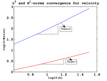
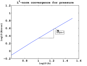
Figure 1: Plot of Convergence Rates for Example 7.1

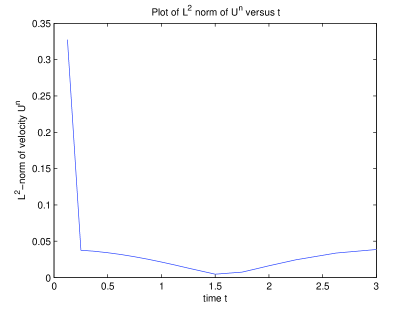
Figure 2: Boundedness of $\|{\bf U}^{n}\|$ as time varies.

Figure 2 depicts that the approximate solution for the data in Example 7.1 is bounded. Note that, here the right hand side function is bounded for all time. Further, Tables 1, 2, 3 represent that the order of convergence for the velocity and pressure errors in Theorems 5.1 and 6.1 hold true in the limit $\kappa\rightarrow 0$.

S No	$h$	$\|{\bf u}(t_{n})-{\bf U}^{n}\|_{\bf{L}^{2}}$	$\|{\bf u}(t_{n})-{\bf U}^{n}\|_{\bf{L}^{2}}$	$\|{\bf u}(t_{n})-{\bf U}^{n}\|_{\bf{L}^{2}}$	$\|{\bf u}(t_{n})-{\bf U}^{n}\|_{\bf{L}^{2}}$
		$\kappa=1$	$\kappa=10^{-3}$	$\kappa=10^{-6}$	$\kappa=10^{-9}$
1	1/4	1.28476	1.46678	1.46699	1.46699
2	1/8	1.66634	1.71546	1.71552	1.71552
3	1/16	1.84754	1.86060	1.86062	1.86062
4	1/32	1.93052	1.93390	1.93391	1.93391

Table 1: Numerical convergence rates for velocity error with variation in $\kappa$ for Example 7.1

S No	$h$	$\|{\bf u}(t_{n})-{\bf U}^{n}\|_{{\bf{H}}^{1}}$	$\|{\bf u}(t_{n})-{\bf U}^{n}\|_{{\bf{H}}^{1}}$	$\|{\bf u}(t_{n})-{\bf U}^{n}\|_{{\bf{H}}^{1}}$	$\|{\bf u}(t_{n})-{\bf U}^{n}\|_{{\bf{H}}^{1}}$
		$\kappa=1$	$\kappa=10^{-3}$	$\kappa=10^{-6}$	$\kappa=10^{-9}$
1	1/4	0.52668	0.70916	0.70938	0.70938
2	1/8	0.80620	0.85510	0.85516	0.85516
3	1/16	0.91745	0.93032	0.93033	0.93033
4	1/32	0.96385	0.96716	0.96716	0.96716

Table 2: Numerical convergence rates for velocity error with variation in $\kappa$ for Example 7.1

S No	$h$	$\|p(t_{n})-P^{n}\|$	$\|p(t_{n})-P^{n}\|$	$\|p(t_{n})-P^{n}\|$	$\|p(t_{n})-P^{n}\|$
		$\kappa=1$	$\kappa=10^{-3}$	$\kappa=10^{-6}$	$\kappa=10^{-9}$
1	1/4	1.25307	1.25165	1.25164	1.25164
2	1/8	1.12462	1.11394	1.11393	1.11393
3	1/16	1.06496	1.05938	1.05937	1.05937
4	1/32	1.02882	1.02663	1.02663	1.02663

Table 3: Numerical convergence rates for pressure error with variation in $\kappa$ for Example 7.1

Example 7.2.

In this example, the initial velocity is chosen as
$u_{1}=10\,\,x^{2}(x-1)^{2}y(y-1)(2y-1),\;\;\;\;u_{2}=-10\,\,y^{2}(y-1)^{2}x(x-1)(2x-1),\;\;\;\;p=40\,\,xy$
with $\nu=1$, $\kappa=1$ and $f=0$. In this case, to obtain the error estimates the exact solution ${\bf u}$ is replaced by finite element solution obtained in a refined mesh.

The convergence rates presented in Figure 3 are in agreement with the results obtained for $f=0$, that is, the convergence rate for velocity in $\bf{L}^{2}$ norm is $\mathcal{O}(h^{2})$, for velocity in ${\bf{H}}^{1}$-norm is $\mathcal{O}(h)$ and for pressure in $L^{2}$ norm is $\mathcal{O}(h)$. In Figure 4, the exponential decay property for the approximate solution $\|{\bf U}^{n}\|$ is shown which verifies theoretical estimates for $f=0$.

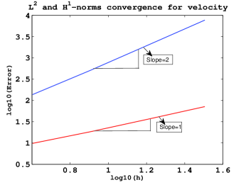
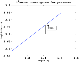
Figure 3: Plot of Convergence Rates for Example 7.2

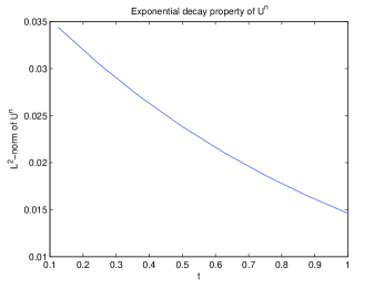
Figure 4: Decay property of $\|{\bf U}^{n}\|$ corresponding to Example 7.2

Example 7.3.

This example demonstrates the exponential decay property of the discrete solution. Here, $\nu=1$, $\kappa=1$ and $f=0$ with ${\bf u}_{0}=\left(\sin^{2}(3\pi x)\sin(6\pi y),-\sin^{2}(3\pi y)\sin(6\pi x),sin(2\pi x)\sin(2\pi y)\right)$ in (1.1)-(1.3). Once again, the error estimates are achieved by considering refined finite element solution as an exact solution.

The order of convergence is shown in Table 4. Figure 5 represents the exponential decay property of $\|{\bf U}^{n}\|$ as time varies which is expected from theoretical analysis for right hand side function $f=0$.

S No	$h$	$\|{\bf u}-{\bf U}^{n}\|_{\bf{L}^{2}}$	Convergence	$\|{\bf u}-{\bf U}^{n}\|_{{\bf{H}}^{1}}$	Convergence
			Rate		Rate
1	1/4	0.430939		6.833152943841204
2	1/8	0.203398	1.083175531775576	5.967502741440636	0.195424
3	1/16	0.065544	1.633758732735566	3.674410879988224	0.699614
4	1/32	0.017502	1.904904362752530	1.917811790943292	0.938051

Table 4: Numerical errors and Convergence rates with $k=h^{2}$ for Example 7.3

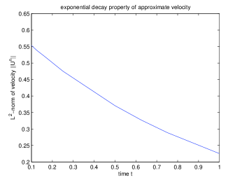
Figure 5: Decay property of $\|{\bf U}^{n}\|$ corresponding to Example 7.3

8 Conclusion

This article in its first part deals with a priori estimates for the weak solution of (1.1)-(1.3) which are valid uniformly in time as $t\mapsto\infty$ and also uniformly for all $\kappa$ as $\kappa\mapsto 0.$ While estimates hold for $2D,$ that is, $d=2,$ and for $3D,$ that is, $d=3,$ estimates are valid with smallness assumption on the data.In the second part, semidiscrete optimal error estimates of order $O(\kappa^{-1/2}h^{m})$ are derived for the velocity in $L^{\infty}(\bf{L}^{2})$-norm when $m=2$ and for the velocity in $L^{\infty}({\bf{H}}^{1}_{0})$-norm, when $m=1$. Moreover for the pressure term, optimal order estimate $L^{\infty}(L^{2})$-norm, which is of order $O(\kappa^{-1/2}h)$ is established. In all these error analyses, constants appeared in the error estimates depend exponentially on $T.$ But, under the uniqueness assumption, it is shown that optimal error estimates are valid uniformly for all time $t>0.$ Further, with $\kappa=O(h^{2\delta}),\;\delta>0$ very small, quasi-optimal error estimates are derived which are valid uniformly in $\kappa$ as $\kappa\mapsto 0.$ All the above results hold true for $2D$, but for $3D$ with smallness assumption on the data. However, in stead of applying Lemma 3.3, if we apply Lemma 3.2, then regularity results like in Theorem 3.1 can be obtained now with constants depending on $1/\kappa,$ but all results are valid for $3D$ without assumption of smallness on the data. Similar conclusion for optimal error estimates can be derived, but with constants depending on $1/\kappa.$ Finally, numerical experiments are conducted to confirm our theoretical findings.

Acknowledgement The authors thank the referee for his/her valuable suggestion which has helped to improve our results.