Analysis of the observed and intrinsic durations of Swift/BAT gamma-ray bursts

Abstract

The duration distribution of 947 GRBs observed by Swift/BAT, as well as its subsample of 347 events with measured redshift, allowing to examine the durations in both the observer and rest frames, are examined. Using a maximum log-likelihood method, mixtures of two and three standard Gaussians are fitted to each sample, and the adequate model is chosen based on the value of the difference in the log-likelihoods, Akaike information criterion and Bayesian information criterion. It is found that a two-Gaussian is a better description than a three-Gaussian, and that the presumed intermediate-duration class is unlikely to be present in the Swift duration data.

1 Introduction

Gamma-ray bursts (GRBs) were detected by military satellites Vela in late 1960’s. Mazets et al. [1981] first pointed out hints for a bimodal distribution of $T_{b}$ (taken to be the time interval within which fall $80\%-90\%$ of the measured GRB’s intensity) drawn for 143 events detected in the KONUS experiment. Burst and Transient Source Explorer (BATSE) onboard the Compton Gamma Ray Observatory (CGRO) provided data that were further investigated by Kouveliotou et al. [1993], and led to establishing the common classification of GRBs into short ($T_{90}<2\,{\rm s}$) and long ($T_{90}>2\,{\rm s}$), where $T_{90}$ is the time during which 90% of the burst’s fluence is accumulated, referred to as the duration of a GRB. The progenitors of long GRBs are associated with supernovae related with collapse of massive stars [Woosley and Bloom, 2006]. Progenitors of short GRBs are thought to be NS-NS or NS-BH mergers [Nakar, 2007], and no connection between short GRBs and supernovae has been proven [Zhang et al., 2009]. It was observed that durations $T_{90}$ seem to exhibit log-normal distributions which were thereafter fitted to short and long GRBs [McBreen et al., 1994, Koshut et al., 1996, Kouveliotou et al., 1996, Horváth, 2002].

The existence of an intermediate-duration GRB class, consisting of GRBs with $T_{90}$ in the range $2-10\,{\rm s}$, was put forward [Horváth, 1998, Mukherjee et al., 1998] based on the analysis of BATSE 3B data. It was supported [Horváth, 2002, Chattopadhyay et al., 2007] with the use of the complete BATSE dataset. Evidence for a third log-normal component was also found in Swift/BAT data [Horváth et al., 2008, Zhang and Choi, 2008, Huja et al., 2009, Horváth et al., 2010]. Interestingly, Zitouni et al. [2015] re-examined the BATSE current catalog as well as the Swift dataset, and found that a mixture of three Gaussians (3-G) fits the $\log T_{90}$ data from Swift better than a two-Gaussian (2-G), while in the case of BATSE statistical tests did not support the presence of a third component (hereinafter, the $\log T_{90}$ distributions are considered, and are shortly referred to as durations as well). Regarding Fermi/GBM [Gruber et al., 2014, von Kienlin et al., 2014], a 3-G is a better fit than a 2-G, however the presence of a third group in the duration distribution was found to be unlikely [Tarnopolski, 2015a, b], which was based on the fact that the $\log T_{90}$ distribution is bimodal, i.e. it exhibits two local maxima [Tarnopolski, 2015a], and that a mixture of two skewed components follows the data better than a standard three-Gaussian [Tarnopolski, 2015b].

The Swift data were re-examined by Bromberg et al. [2013], and they found that a limit of $0.8\,{\rm s}$ is more suitable for the GRBs observed by Swift than the conventional $2\,{\rm s}$ limit of Kouveliotou et al. [1993]. It should be stressed that Bromberg et al. [2013] applied a different approach than Kouveliotou et al. [1993] and Tarnopolski [2015c]: a functional form of the $T_{90}$ distribution different from the commonly used phenomenological log-normal distribution, coming from a physical model for the short duration collapsar distribution, and by means of exceeding a probability threshold that a GRB with a given $T_{90}$ is a non-collapsar. Interestingly, the limits for BATSE and Fermi data are consistent with the $2\,{\rm s}$ limit, and also with the results obtained by Tarnopolski [2015c], where based on the well-established conjecture that durations $T_{90}$ are log-normally distributed, the limit between short and long GRBs may be placed at the local minimum, which is detector-dependent. Finally, many works in which a 2-G was fitted to the $\log T_{90}$ distribution showed a significant overlap of components corresponding to short and long GRBs [McBreen et al., 1994, Koshut et al., 1996, Horváth, 2002, Zhang and Choi, 2008, Huja et al., 2009, Bromberg et al., 2013, Barnacka and Loeb, 2014, Tarnopolski, 2015c, Zitouni et al., 2015].

The aim of this paper is to analyze the current dataset of Swift/BAT GRBs, and to test whether a greater sample of 947 events leads to conclusions other than Zitouni et al. [2015] arrived at for a set of 757 events. Moreover, a relevant increase of GRBs with measured redshift—347 compared to 248 GRBs examined by Zitouni et al. [2015]—provides an opportunity for a re-evaluation of the GRB properties that are, after moving to the rest frame, not affected by cosmological factors. This paper is organized in the following manner. In Section 2 the datasets, fitting method and statistical criteria used to infer the validity of the models applied are described. Section 3 presents the results of fitting a 2-G and 3-G to the whole sample of 947 GRBs, as well as a subsample of 347 events in both the observer and rest frames. Section 4 is devoted to discussion, and gathers concluding remarks.

2 Methods

2.1 Dataset

The Swift dataset contains 947 GRBs with measured duration $T_{90}$, of which 9% are short (87 events). 347 GRBs have their redshift known, and those constitute the second sample examined herein. It consists of 324 long GRBs and 23 short ones. A scatter plot of this subsample on a $\log T_{90}-z$ plane is drawn in Fig. 1. The median redshift for short and long GRBs is equal to $\tilde{z}_{\rm short}=0.72$ and $\tilde{z}_{\rm long}=1.90$, respectively. The intrinsic durations are calculated according to

$$T^{\rm int}_{90}=\frac{T^{\rm obs}_{90}}{1+z}.$$ (1)

Distributions of the $\log T_{90}$ for the observed and intrinsic durations are examined hereinafter, and are displayed together with the distribution of the whole sample in Fig. 2.

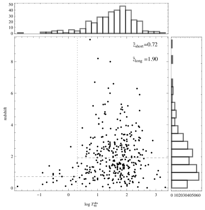
Figure 1: A scatter plot of the redshift versus the observed duration of the Swift subsample. Vertical dotted line denotes the limitting value of $2\,{\rm s}$ between short and long GRBs, and the horizontal dashed lines mark the medians of the respective classes, with values written in the plot.

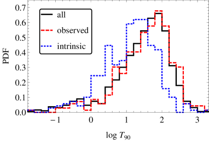
Figure 2: Distributions of the examined samples: the whole sample (solid black); observed (dashed red) and intrinsic (dotted blue) durations in the subsample of GRBs with known redshift. The distributions of observed durations for both samples (all GRBs and those with measured redshift) are similar to each other.

2.2 Fitting method

Two standard fitting techniques are commonly applied: $\chi^{2}$ fitting [Voinov et al., 2013] and maximum likelihood (ML, Kendall and Stuart 1973). For the first, data needs to be binned, and despite various binning rules are known (e.g. Freedman-Diaconis, Scott, Knuth etc.), they still leave place for ambiguity, as it might happen that the fit may be statistically significant on a given significance level for a number of binnings [Huja et al., 2009, Koen and Bere, 2012, Tarnopolski, 2015a]. The ML method is not affected by this issue and is therefore applied herein. However, for display purposes, the binning was chosen based on the Freedman-Diaconis rule.

Having a distribution with a probability density function (PDF) given by $f=f(x;\theta)$ (possibly a mixture), where $\theta=\left\{\theta_{i}\right\}_{i=1}^{p}$ is a set of parameters, the log-likelihood function is defined as

$$\mathcal{L}_{p}(\theta)=\sum\limits_{i=1}^{N}\ln f(x_{i};\theta),$$ (2)

where $\left\{x_{i}\right\}_{i=1}^{N}$ are the datapoints from the sample to which a distribution is fitted. The fitting is performed by searching a set of parameters $\hat{\theta}$ for which the log-likelihood is maximized. When nested models are considered, the maximal value of the log-likelihood function $\mathcal{L}_{\rm max}\equiv\mathcal{L}_{p}(\hat{\theta})$ increases when the number of parameters $p$ increases.

A mixture of $k$ standard normal (Gaussian) distributions:

$$f_{k}(x)=\sum\limits_{i=1}^{k}\frac{A_{i}}{\sqrt{2\pi}\sigma_{i}}\exp\left(-\frac{(x-\mu_{i})^{2}}{2\sigma_{i}^{2}}\right),$$ (3)

is considered. It is described by $p=3k-1$ free parameters: $k$ pairs $(\mu_{i},\sigma_{i})$ and $k-1$ weights $A_{i}$, satysfying $\sum_{i=1}^{k}A_{i}=1$ due to normalization of a PDF. Therefore, $p=5$ for a 2-G, and $p=8$ for a 3-G.

2.3 Statistical criteria

If one has two fits such that $\mathcal{L}_{p_{2},{\rm max}}>\mathcal{L}_{p_{1},{\rm max}}$, then twice their difference, $2\Delta\mathcal{L}_{\rm max}=2(\mathcal{L}_{p_{2},{\rm max}}-\mathcal{L}_{p_{1},{\rm max}})$, is distributed like $\chi^{2}(\Delta p)$, where $\Delta p=p_{2}-p_{1}>0$ is the difference in the number of parameters [Kendall and Stuart, 1973, Horváth, 2002]. If a $p$-value associated with the value of $\chi^{2}(\Delta p)$ does not exceed the significance level $\alpha$, one of the fits (with higher $\mathcal{L}_{\rm max}$) is statistically better than the other. For instance, for a 2-G and a 3-G, $\Delta p=3$, and despite that, according to Footnote 1, $\mathcal{L}_{\rm max,\,3-G}>\mathcal{L}_{\rm max,\,2-G}$ holds always, twice their difference provides a decisive $p$-value.

For nested as well as non-nested models, the Akaike information criterion ($AIC$) [Akaike, 1974, Burnham and Anderson, 2004, Liddle, 2007] may be applied. The $AIC$ is defined as

$$AIC=2p-2\mathcal{L}_{p,{\rm max}}.$$ (4)

A preferred model is the one that minimizes $AIC$. The formulation of $AIC$ penalizes the use of an excessive number of parameters, hence discourages overfitting. It prefers models with fewer parameters, as long as the others do not provide a substantially better fit. The expression for $AIC$ consists of two competing terms: the first measuring the model complexity (number of free parameters), and the second measuring the goodness of fit (or more precisely, the lack of thereof). Among candidate models with $AIC_{i}$, let $AIC_{\rm min}$ denote the smallest. Then,

$$Pr_{i}=\exp\left(-\frac{\Delta_{i}}{2}\right),$$ (5)

where $\Delta_{i}=AIC_{i}-AIC_{\rm min}$, can be interpreted as the relative (compared to $AIC_{\rm min}$) probability that the $i$th model minimizes the $AIC$.

The $AIC$ is suitable when $N/p$ is large, i.e. when $N/p>40$ [Burnham and Anderson, 2004, see also references therein]. When this condition is not fulfilled, a second order bias correction is introduced, resulting in a small-sample version of the $AIC$, called $AIC_{c}$:

$$AIC_{c}=2p-2\mathcal{L}_{p,{\rm max}}+\frac{2p(p+1)}{N-p-1}.$$ (6)

The relative probability is computed similarly to when $AIC$ is used, i.e. Eq. (5) is valid when one takes $\Delta_{i}=AIC_{c,i}-AIC_{c,{\rm min}}$. Thence,

$$Pr_{i}=\exp\left(-\frac{AIC_{c,i}-AIC_{c,{\rm min}}}{2}\right).$$ (7)

Obviously, $AIC_{c}$ converges to $AIC$ when $N$ is large.

It is important to note that this method allows to choose a model that is best among a given set, but does not allow to state that this model is the best among all possible ones. Hence, the probabilities computed by means of Eq. (7) are the relative (with respect to a model with $AIC_{c,{\rm min}}$) probabilities that the data is better described by a model with $AIC_{c,i}$. What is essential in assesing the goodness of a fit in the $AIC$ method is the difference, $\Delta_{i}=AIC_{c,i}-AIC_{c,{\rm min}}$, not the absolute value of an $AIC_{c,i}$. If $\Delta_{i}<2$, then there is substantial support for the $i$th model, and the proposition that it is a proper description is highly probable. If $2<\Delta_{i}<4$, then there is strong support for the $i$th model. When $4<\Delta_{i}<7$, there is considerably less support, and models with $\Delta_{i}>10$ have essentially no support [Burnham and Anderson, 2004].

The Bayesian information criterion ($BIC$) was introduced by Schwarz [1978], and is defined as

$$BIC=p\ln N-2\mathcal{L}_{p,{\rm max}}.$$ (8)

As was the case in the $AIC$ (or $AIC_{c}$), a preferred model is the one that minimizes $BIC$, which also penalizes the usage of an excessive number of free parameters. The most striking difference between the two is that the penalization term, $k\ln N$, is greater than the corresponding term from the $AIC$, i.e. $2p$, for $N\geq 8$. Hence, the penalization in case of the $BIC$ is much more stringent, especially for large samples.

The probability in favor of the $i$th model, relative to a model with $BIC_{\rm min}$, is defined in the same manner as it was for $AIC$:

$$Pr_{i}=\exp\left(-\frac{\Delta_{i}}{2}\right),$$ (9)

where $\Delta_{i}=BIC_{i}-BIC_{\rm min}$ in this case, and the support for the $i$th model (or evidence against it) also depends on the differences: if $\Delta_{i}<2$, then there is substantial support for the $i$th model (or the evidence against it is worth only a bare mention). When $2<\Delta_{i}<6$, then there is positive evidence against the $i$th model. If $6<\Delta_{i}<10$, the evidence is strong, and models with $\Delta_{i}>10$ yield a very strong evidence against the $i$th model (essentially no support, Kass and Raftery 1995).

Despite apparent similarities between the $AIC$ and $BIC$, they answer different questions, as they are derived based on different assumptions. $AIC$ tries to select a model that most adequately describes reality (in the form of the data under examination). This means that in fact the model being a real description of the data is never considered. On the contrary, $BIC$ tries to find the true model among the set of candidates. Because $BIC$ is more stringent, it has a tendency to underfit, while $AIC$, as a more liberal method, is inclined towards overfitting. This leads sometimes to pointing different models by the two criteria, which happens rarely, but is due to the fact that they try to satisfy different conditions.

3 Results

3.1 All Swift GRBs

Using the ML method from Sect. 2.2, the fitting of a 2-G and 3-G to the duration distribution of 947 GRBs is performed. The results, in graphical form, are shown in Fig. 3. The two-component mixture is unimodal, but with a prominent tail on the left side. The three-component fit is bimodal, with a clear shoulder on the left side of the peak related to long GRBs. The local minimum is placed at $T_{90}=1.07\,{\rm s}$. It is interesting to note that this value is consistent with the short-long GRB limit from Bromberg et al. [2013]. The overall shape of the curve is in agreement with previous results [Horváth et al., 2008, Zhang and Choi, 2008, Tarnopolski, 2015b, Zitouni et al., 2015].

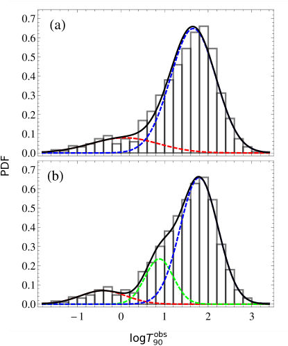
Figure 3: Distributions fitted to $\log T^{\rm obs}_{90}$ of all Swift GRBs. Color dashed curves are the components of the (black solid) mixture distribution. The panels show mixtures of (a) two and (b) three standard Gaussians.

The parameters of the fits are gathered in Table 1. Twice the difference in $\mathcal{L}_{p,{\rm max}}$ is equal to 22.336, what corresponds to a $p$-value of $6\times 10^{-5}$, indicating that a 3-G is a highly significant improvement over a 2-G. This is confirmed with the $AIC_{c}$ approach, as their difference is equal to 16.246, what gives a probability of $3\times 10^{-4}$ that the 2-G might in fact be a better description than a 3-G. However, the results of the $BIC$ give a much lower significance—the difference is only 1.776, corresponding to a probability of 0.41 in favor of the 2-G. Nevertheless, all criteria pointed at a 3-G as a better model among the two under consideration.

Table 1: Parameters of the fits for the observed durations of 947 Swift GRBs. The values in favor of a respective model are marked in bold.

$i$	$\mu_{i}$	$\sigma_{i}$	$A_{i}$	$\mathcal{L}_{\rm max}$	$AIC_{c}$	$BIC$
1	0.083	0.781	0.155	$-1035.351$	2080.765	2104.968
2	1.657	0.521	0.845
1	$-0.407$	0.529	0.093
2	0.878	0.322	0.190	$-$1024.183	2064.519	2103.192
3	1.793	0.434	0.717

3.2 Subsample of Swift GRBs with measured redshift

3.2.1 Observed durations

The observed durations of the redshift-equipped GRB subsample are examined in the same way as in the previous Section 3.1. The fitted curves, displayed in Fig. 4, resemble the ones obtained for the complete GRB sample. The fitted parameters, gathered in Table 2, are in good agreement, too. The difference in $\mathcal{L}_{p,{\rm max}}$ multiplied by two, being equal to 6.522, corresponds to a relatively high probability of 0.09. The difference in $AIC_{c}$, equal to 0.270, is negligible, and hence based on it one can not rule out any of the fits—the relative probability is 0.87. On the other hand, the lower $BIC$ was achieved by a 2-G, and the difference is a prominent 11.027, which gives a probability of $4\times 10^{-3}$. Hence, the overall evidence against a 3-G is very strong—it follows that based on $BIC$, a 2-G is a better model.

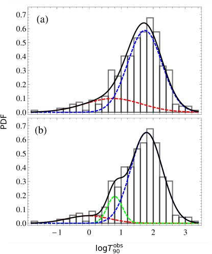
Figure 4: The same as Fig. 3, but for a subsample of GRBs with measured redshift.

Table 2: Parameters of the fits for the observed durations of 347 Swift GRBs with measured redshift.

$i$	$\mu_{i}$	$\sigma_{i}$	$A_{i}$	$\mathcal{L}_{\rm max}$	$AIC_{c}$	$BIC$
1	0.745	0.894	0.221	$-372.281$	754.737	773.808
2	1.739	0.530	0.779
1	$-0.019$	0.664	0.089
2	0.803	0.236	0.114	$-$369.020	754.467	784.835
3	1.793	0.434	0.797

3.2.2 Intrinsic durations

In the case of the intrinsic durations, the fits displayed in Fig. 5 reveal a systematic shift, compared to the distribution of $T^{\rm obs}_{90}$, towards shorter durations. While a 2-G is again unimodal and skewed leftwards, the 3-G shows a peak at $T_{90}=1.42\,{\rm s}$, between the regions of short and long GRBs. The parameters of the fits are gathered in Table 3.

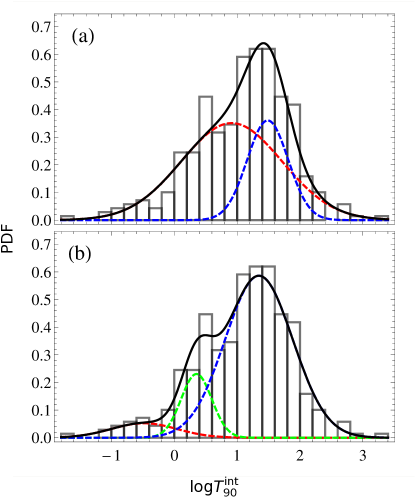
Figure 5: The same as Fig. 4, but in the rest frame.

The doubled difference of $\mathcal{L}_{p,{\rm max}}$ is equal to 1.504, what implies a high relative probability of 0.68. The difference in $AIC_{c}$ is 4.747, what hints toward a 2-G with a relative probability of 0.09 that a 3-G is in fact a better model. In this case, the $BIC$ yield a difference of 16.045, which gives a strong support in favor of a 2-G. The relative probability that the 3-G might be the more appropriate description of the data, is only $3\times 10^{-4}$. Overall, the $AIC_{c}$ and $BIC$ are in agreement, and without taking into account the doubled difference of $\mathcal{L}_{p,{\rm max}}$, because it provides no evidence in favor of any model, it turns out that a 2-G is a better model than a 3-G.

Table 3: Parameters of the fits for the intrinsic durations of 347 Swift GRBs.

$i$	$\mu_{i}$	$\sigma_{i}$	$A_{i}$	$\mathcal{L}_{\rm max}$	$AIC_{c}$	$BIC$
1	0.913	0.802	0.705	$-379.644$	769.463	788.534
2	1.487	0.326	0.295
1	$-0.480$	0.521	0.068
2	0.353	0.244	0.141	$-$378.892	774.210	804.579
3	1.347	0.538	0.791

4 Discussion and conclusions

The duration distribution of 947 GRBs observed by Swift, and a subsample consisting of 347 events with measured redshift, were investigated. The redshifts allowed to examine the intrinsic durations, i.e. in the rest frame, as well. Mixtures of two and three standard Gaussians were fitted. For each sample, the best fit was chosen based on the value of the difference in the log-likelihoods doubled, Akaike information criterion and Bayesian information criterion. The main conclusions are as follows:

1. All three criteria point at a 3-G as an adequate description of the $\log T_{90}$ distribution of all 947 Swift GRBs. The fit is bimodal, what is in good agreement with the two well established populations (mergers for short, and collapsars for long GRBs). This might suggest that the commonly applied log-normal distribution is not a good model for the observed duration distribution.

2. For a subsample of 347 GRBs with measured redshift, the analyses of the observed and intrinsic durations yielded results being in quite good agreement. While only the $BIC$ hints at a unimodal 2-G in the case of $\log T^{\rm obs}_{90}$, the other two criteria did not yield support for any of the models strong enough to infer their plausibility, but with a low ratio of short to long GRBs ($<1:14$) in this Swift subsample, combined with the well known overlap of durations of short and long GRBs and the relative smallness of the subsample, this is not that surprising.

3. The intrinsic durations, $\log T^{\rm int}_{90}$, are best described by a unimodal 2-G, too. Both $AIC_{c}$ and $BIC$ yield strong support in favor of a two-component Gaussian, while the criterion based on log-likelihoods did not provide a conclusive outcome. Hence, in all three samples the presence of two populations was found to be likely, and the evidence against a three-component description is strong.

4. In case of $T^{\rm obs}_{90}$ in the redshift-equipped subsample of 347 GRBs, the $AIC_{c}$ and $BIC$ lead to different conclusions: the $AIC_{c}$ pointed at a 3-G (with very weak evidence against a 2-G though), and $BIC$ yielded a very strong support for the 2-G. While this seems to be contradictive, it needs to be interpreted in the context of each criterion: according to $AIC_{c}$, a 3-G is a slightly better choice in describing the data, and because the difference in the models is negligible, the $BIC$ strongly favors the simpler one, i.e. the one with fewer parameters. This illustrates that any statistical criterion can not be a stand-alone determinant in inferring the underlying model, but (i) needs to be interpreted in the light of its conditions, and (ii) it is useful to apply different tools and analyze their output in relation to each other.

References

References

- Akaike [1974] Akaike H. A New Look at the Statistical Model Identification. IEEE Transactions on Automatic Control 1974;19:716–23.
- Barnacka and Loeb [2014] Barnacka A, Loeb A. A Size-duration Trend for Gamma-Ray Burst Progenitors. Astrophysical Journal Letters 2014;794:L8. doi:10.1088/2041-8205/794/1/L8.
- Biesiada [2007] Biesiada M. Information theoretic model selection applied to supernovae data. Journal of Cosmology and Astroparticle Physics 2007;2:3. doi:10.1088/1475-7516/2007/02/003.
- Bromberg et al. [2013] Bromberg O, Nakar E, Piran T, Sari R. Short versus Long and Collapsars versus Non-collapsars: A Quantitative Classification of Gamma-Ray Bursts. Astrophysical Journal 2013;764:179. doi:10.1088/0004-637X/764/2/179.
- Burnham and Anderson [2004] Burnham KP, Anderson DR. Multimodel inference: understanding AIC and BIC in Model Selection. Sociological Methods and Research 2004;33:261–304. doi:10.1177/0049124104268644.
- Chattopadhyay et al. [2007] Chattopadhyay T, Misra R, Chattopadhyay AK, Naskar M. Statistical Evidence for Three Classes of Gamma-Ray Bursts. Astrophysical Journal 2007;667:1017–23. doi:10.1086/520317.
- Gruber et al. [2014] Gruber D, Goldstein A, Weller von Ahlefeld V, Narayana Bhat P, Bissaldi E, Briggs MS, Byrne D, Cleveland WH, Connaughton V, Diehl R, Fishman GJ, Fitzpatrick G, Foley S, Gibby M, Giles MM, Greiner J, Guiriec S, van der Horst AJ, von Kienlin A, Kouveliotou C, Layden E, Lin L, Meegan CA, McGlynn S, Paciesas WS, Pelassa V, Preece RD, Rau A, Wilson-Hodge CA, Xiong S, Younes G, Yu HF. The Fermi GBM Gamma-Ray Burst Spectral Catalog: Four Years of Data. Astrophysical Journal Supplement 2014;211:12. doi:10.1088/0067-0049/211/1/12.
- Horváth [1998] Horváth I. A Third Class of Gamma-Ray Bursts? Astrophysical Journal 1998;508:757–9. doi:10.1086/306416. arXiv:astro-ph/9803077.
- Horváth [2002] Horváth I. A further study of the BATSE Gamma-Ray Burst duration distribution. Astronomy and Astrophysics 2002;392:791--3. doi:10.1051/0004-6361:20020808.
- Horváth et al. [2010] Horváth I, Bagoly Z, Balázs LG, de Ugarte Postigo A, Veres P, Mészáros A. Detailed Classification of Swift ’s Gamma-ray Bursts. Astrophysical Journal 2010;713:552--7. doi:10.1088/0004-637X/713/1/552.
- Horváth et al. [2008] Horváth I, Balázs LG, Bagoly Z, Veres P. Classification of Swift’s gamma-ray bursts. Astronomy and Astrophysics 2008;489:L1--4. doi:10.1051/0004-6361:200810269.
- Huja et al. [2009] Huja D, Mészáros A, Řípa J. A comparison of the gamma-ray bursts detected by BATSE and Swift. Astronomy and Astrophysics 2009;504:67--71. doi:10.1051/0004-6361/200809802.
- Kass and Raftery [1995] Kass RE, Raftery AE. Bayes Factors. Journal of the American Statistical Association 1995;90:773--95. doi:10.1080/01621459.1995.10476572.
- Kendall and Stuart [1973] Kendall M, Stuart A. The advanced theory of statistics. London: Griffin, 3rd ed., 1973.
- Koen and Bere [2012] Koen C, Bere A. On multiple classes of gamma-ray bursts, as deduced from autocorrelation functions or bivariate duration/hardness ratio distributions. Monthly Notices of the Royal Astronomical Society 2012;420:405--15. doi:10.1111/j.1365-2966.2011.20045.x.
- Koshut et al. [1996] Koshut TM, Paciesas WS, Kouveliotou C, van Paradijs J, Pendleton GN, Fishman GJ, Meegan CA. Systematic Effects on Duration Measurements of Gamma-Ray Bursts. Astrophysical Journal 1996;463:570. doi:10.1086/177272.
- Kouveliotou et al. [1996] Kouveliotou C, Koshut T, Briggs MS, Pendleton GN, Meegan CA, Fishman GJ, Lestrade JP. Correlations between duration, hardness and intensity in GRBs. In: Kouveliotou C, Briggs MF, Fishman GJ, editors. American Institute of Physics Conference Series. volume 384 of American Institute of Physics Conference Series; 1996. p. 42--6. doi:10.1063/1.51695.
- Kouveliotou et al. [1993] Kouveliotou C, Meegan CA, Fishman GJ, Bhat NP, Briggs MS, Koshut TM, Paciesas WS, Pendleton GN. Identification of two classes of gamma-ray bursts. Astrophysical Journal Letters 1993;413:L101--4. doi:10.1086/186969.
- Liddle [2007] Liddle AR. Information criteria for astrophysical model selection. Monthly Notices of the Royal Astronomical Society 2007;377:L74--8. doi:10.1111/j.1745-3933.2007.00306.x.
- Mazets et al. [1981] Mazets EP, Golenetskii SV, Ilinskii VN, Panov VN, Aptekar RL, Gurian IA, Proskura MP, Sokolov IA, Sokolova ZI, Kharitonova TV. Catalog of cosmic gamma-ray bursts from the KONUS experiment data. I. Astrophysics and Space Science 1981;80:3--83. doi:10.1007/BF00649140.
- McBreen et al. [1994] McBreen B, Hurley KJ, Long R, Metcalfe L. Lognormal Distributions in Gamma-Ray Bursts and Cosmic Lightning. Monthly Notices of the Royal Astronomical Society 1994;271:662.
- Mukherjee et al. [1998] Mukherjee S, Feigelson ED, Jogesh Babu G, Murtagh F, Fraley C, Raftery A. Three Types of Gamma-Ray Bursts. Astrophysical Journal 1998;508:314--27. doi:10.1086/306386.
- Nakar [2007] Nakar E. Short-hard gamma-ray bursts. Physics Reports 2007;442:166--236. doi:10.1016/j.physrep.2007.02.005.
- Schwarz [1978] Schwarz G. Estimating the dimension of a model. The Annals of Statistics 1978;6(2):461--4. doi:10.1214/aos/1176344136.
- Tarnopolski [2015a] Tarnopolski M. Analysis of Fermi gamma-ray burst duration distribution. Astronomy and Astrophysics 2015a;581:A29. doi:10.1051/0004-6361/201526415.
- Tarnopolski [2015b] Tarnopolski M. Analysis of gamma-ray burst duration distribution using mixtures of skewed distributions. ArXiv e-prints 2015b;arXiv:1506.07801.
- Tarnopolski [2015c] Tarnopolski M. On the limit between short and long GRBs. Astrophysics and Space Science 2015c;359:20. doi:10.1007/s10509-015-2473-6.
- Voinov et al. [2013] Voinov V, Nikulin M, Balakrishnan N. Chi-Squared Goodness of Fit Tests with Applications. Academic Press, New York, 2013.
- von Kienlin et al. [2014] von Kienlin A, Meegan CA, Paciesas WS, Bhat PN, Bissaldi E, Briggs MS, Burgess JM, Byrne D, Chaplin V, Cleveland W, Connaughton V, Collazzi AC, Fitzpatrick G, Foley S, Gibby M, Giles M, Goldstein A, Greiner J, Gruber D, Guiriec S, van der Horst AJ, Kouveliotou C, Layden E, McBreen S, McGlynn S, Pelassa V, Preece RD, Rau A, Tierney D, Wilson-Hodge CA, Xiong S, Younes G, Yu HF. The Second Fermi GBM Gamma-Ray Burst Catalog: The First Four Years. Astrophysical Journal Supplement 2014;211:13. doi:10.1088/0067-0049/211/1/13.
- Woosley and Bloom [2006] Woosley SE, Bloom JS. The Supernova Gamma-Ray Burst Connection. Annual Review of Astronomy and Astrophysics 2006;44:507--56. doi:10.1146/annurev.astro.43.072103.150558.
- Zhang et al. [2009] Zhang B, Zhang BB, Virgili FJ, Liang EW, Kann DA, Wu XF, Proga D, Lv HJ, Toma K, Mészáros P, Burrows DN, Roming PWA, Gehrels N. Discerning the Physical Origins of Cosmological Gamma-ray Bursts Based on Multiple Observational Criteria: The Cases of z = 6.7 GRB 080913, z = 8.2 GRB 090423, and Some Short/Hard GRBs. Astrophysical Journal 2009;703:1696--724. doi:10.1088/0004-637X/703/2/1696.
- Zhang and Choi [2008] Zhang ZB, Choi CS. An analysis of the durations of Swift gamma-ray bursts. Astronomy and Astrophysics 2008;484:293--7. doi:10.1051/0004-6361:20079210.
- Zitouni et al. [2015] Zitouni H, Guessoum N, Azzam WJ, Mochkovitch R. Statistical study of observed and intrinsic durations among BATSE and Swift/BAT GRBs. Astrophysics and Space Science 2015;357:7. doi:10.1007/s10509-015-2311-x.