Loading-unloading hysteresis loop of randomly rough adhesive contacts.

Abstract

In this paper we investigate the loading and unloading behavior of soft solids in adhesive contact with randomly rough profiles. The roughness is assumed to be described by a self-affine fractal on a limited range of wave-vectors. A spectral method is exploited to generate such randomly rough surfaces. The results are statistically averaged, and the calculated contact area and applied load are shown as a function of the penetration, for loading and unloading conditions. We found that the combination of adhesion forces and roughness leads to a hysteresis loading-unloading loop. This shows that energy can be lost simply as a consequence of roughness and van der Waals forces, as in this case a large number of local energy minima exist and the system may be trapped in metastable states. We numerically quantify the hysteretic loss and assess the influence of the surface statistical properties and the energy of adhesion on the hysteresis process.

I Introduction

Contact mechanics between rough surfaces plays a crucial role in a large number of engineering applications, ranging from seals Persson-2008 ; Lorenz-2010 , boundary and mixed lubrication Scaraggi-2011 ; Scaraggi-2011BIS , adhesive systems and friction Carbone-2008 ; Zhao-2003 ; Carbone-2013 . Recently, an increasing interest in these topics has been motivated by the increasing efforts made to face up new technological challenges, such as the manufacturing of novel bio-inspired adhesives Geim-2003 ; Carbone-2011 ; Carbone-2012 , the optimization of seals Bottiglione-2009 ; Dapp-2012 , the extreme downsizing of mechanical and electrical devices. In particular, micro- and nano-mechanical systems (MEMS/NEMS) have driven the development of new materials and surfaces, involving an increasing influence of surface phenomena. In such applications, where usually surfaces may experience rapid intermittent contacts, it is then very important to know how adhesion and roughness affect the behavior of the system and in particular the energy dissipation at the interface. This aspect of the problem is also very critical when scanning probe microscopy, as atomic force microscopy (AFM), is utilized to characterize the mechanical behavior and surface properties of materials. During adhesive contacts of rough solids the measured contact force versus displacement shows a clear hysteretic loop associated with energy dissipation Pickering-2001 ; Chen-1991 ; Maeda-2002 , which is not observed in perfectly smooth elastic contacts.

The relevance of the problem have strongly stimulated this research field. However, notwithstanding the quite large amount of papers dealing with the adhesive contact of rough surfaces FullerTabor-1975 ; Pastewka-2014 ; Hyun-2004 ; Luan-2009 ; Jackson-2011 ; Medina-2014 ; Medina-2013 ; Sellgren-2003 , only a few papers attempt to explain the origin of adhesion hysteresis and energy dissipation in rough contacts Li-2015 ; Kadin-2006 ; Kadin-2008 . This is usually attributed to the presence of plasticity Eid-2011 ; Kadin-2006 ; Kadin-2008 , interdigitations among polymer chains Maeda-2002 , humidity Pickering-2001 , viscoelasticity Tirrell-1996 ; Greenwood-1981 . In fact all these phenomena can act contemporaneously, so that distinguishing among the different causes has become of utmost importance. Only a few works have made an effort in such direction. For example Refs. Guduru-2007 ; Guduru-2007BIS ; Zappone-2007 ; Kesari-2010 proved that adhesion hysteresis can be observed even in the case of elastic solids provided that the contact occurs between rough surfaces.The study presented herewith aims to provide an additional contribution along this direction. By employing a methodology based on a pure continuum mechanics approach, which belongs to the class of Boundary Element Methods (BEMs) Carbone-2008 ; Carbone-2012 ; Carbone-2009 , we analyse numerically the loading-unloading adhesive contact of rough solids by including adhesion in terms of surface energy, i.e. by assuming that the range of the adhesive interaction is infinitely short. We study, in particular, the influence of adhesion and surface roughness on the hysteresis loop, and show that energy can be lost simply as a consequence of roughness and van der Waals forces. Such energy loss is numerically quantified and explained in terms of two different but concurrent mechanisms occurring at the contact interface and involving different ranges of roughness length scales.

II The numerical model

We briefly summarize the numerical methodology presented in Carbone-2008 ; Carbone-2012 ; Carbone-2009 . We consider a periodic problem where an elastic half-space is in contact with a randomly rough rigid profile of height distribution $h\left(x\right)$ as shown in Fig. 1, where $\lambda$ is the spatial period of the profile. The quantity $h\left(x\right)$ is the height of the profile measured from its mean plane. Because of periodicity $h\left(x\right)$ can be represented in exponential form as

$$h\left(x\right)={\displaystyle\sum\limits_{m=-\infty}^{+\infty}}a\left(q_{m}\right)e^{iq_{m}x}={\displaystyle\sum\limits_{m=-\infty}^{+\infty}}a_{m}e^{imq_{0}x}$$ (1)

Figure 1: An elastic half-space in contact with a periodic randomly rough rigid substrate of wavelength $\lambda$.

where the fundamental wavevector $q_{0}=2\pi/\lambda$, $m$ is the wavenumber, $a_{m}=\left|a_{m}\right|e^{i\phi_{m}}$ and $\phi_{m}$ the phase of the $m$-th spectral component, uniformly distributed in the interval $\left[0,2\pi\right[$. Figure 2 shows the total displacement $u_{\mathrm{tot}}$ of the substrate, the average displacement $u_{\mathrm{m}}$ of the boundary of the deformed layer, and the penetration $\Delta$ of the rigid substrate into the elastic layer. These three quantities are shown to satisfy the following relation

$$u_{\mathrm{tot}}=\Delta+u_{\mathrm{m}}$$ (2)

Figure 2: A schematic representation of elastic displacement field at the interface, as they occur during approaching the substrate to the elastic solid by a quantity $u_{\mathrm{tot}}$. Observe that $u_{\mathrm{tot}}$ is the sum of the mean displacement $u_{\mathrm{m}}$ of the elastic body and substrate penetration $\Delta$. Also the interfacial displacement and the separation $s$ between the two surfaces are shown.

Figure 2 also shows the so called interfacial displacement $v\left(x\right)$, and the separation $s=h_{\max}-\Delta$ between the two surfaces, where $h_{\max}=\max\left[h\left(x\right)\right]$ is the maximum height of the roughness from its mean plane. Let us define the contact domain $\mathrm{\Omega}=\cup_{i=1}^{L}\left[a_{i},b_{i}\right]$, where $a_{i}$ and $b_{i}$ are the coordinates of $i$-th contact patch with $a_{i}<b_{i}$ and $i=1,2,...,L$, where $L$ is the number of contacts patches. Recalling that the interfacial pressure distribution $\sigma\left(x\right)$ vanishes out of the contact domain the relation between $\sigma\left(x\right)$ and the interfacial displacement $v\left(x\right)$ is

$$-\int_{\mathrm{\Omega}}\mathcal{G}\left(x-x^{\prime}\right)\sigma\left(x^{\prime}\right)dx^{\prime}=v\left(x\right)$$ (3)

where the kernel Carbone-2008 ; Carbone-2009

$$\mathcal{G}\left(x\right)=\frac{2\left(1-\nu^{2}\right)}{\pi E}\log\left[2\left|\sin\left(\frac{kx}{2}\right)\right|\right]$$ (4)

represents the Green function of the semi-infinite elastic body under a periodic loading, i.e. it represents the interfacial displacement $v\left(x\right)$ caused by the application of a Dirac comb with peaks $\delta\left(x-n\lambda\right)$ separated by a distance $\lambda$. Here $E$ and $\nu$ are Young’s modulus and Poisson’s ratio of the elastic layer. Now let us define the separation between the elastic solid and the rigid rough substrate, i.e. the distance between the mean plane of the deformed surface and the mean plane of the rough surface, as $s=h_{\max}-\Delta$ (see Fig.2). Noting that in the contact domain $v\left(x\right)=h\left(x\right)-s=h\left(x\right)-h_{\max}+\Delta$ one can also write

$$-\int_{\mathrm{\Omega}}\mathcal{G}\left(x-s\right)\sigma\left(s\right)ds =h\left(x\right)-s;\qquad x\in\mathrm{\Omega}$$ (5)

$$-\int_{\mathrm{\Omega}}\mathcal{G}\left(x-s\right)\sigma\left(s\right)ds =v\left(x\right);\qquad x\notin\mathrm{\Omega}$$ (6)

Eq. (5) is a Fredholm integral equation of the first kind used to determine the unknown pressure distribution in the contact area $\mathrm{\Omega}$. Whereas Eq. (6) is employed to calculate the displacement $v\left(x\right)$ out of the contact area by simply performing the integral at the left hand side. In order to close the system of equations we need an additional condition to determine the yet unknown contact domain $\mathrm{\Omega}$. To this end, we first observe that for any penetration $\Delta$ or equivalently for any given separation $s$, we can calculate the pressure distribution at the interface through Eq. (5), and the interfacial elastic displacement through Eq. (6), as functions of the unknown coordinates $a_{i}$ and $b_{i}$ of the $i$-th contact area. To calculate the exact values of the quantities $a_{i}$ and $b_{i}$ at equilibrium we need to minimize the interfacial free energy $U_{\mathrm{tot}}\left(a_{1},b_{1},...,a_{L},b_{L},\Delta\right)$ of the system at fixed penetration $\Delta$ Carbone-2008 ; Carbone-2009 .

The free interfacial energy is

$$U_{\mathrm{tot}}=U_{\mathrm{el}}+U_{\mathrm{ad}}$$ (7)

where the interfacial elastic energy $U_{\mathrm{el}}$ is Carbone-2008 ; Carbone-2009

$$U_{\mathrm{el}}\left(a_{1},b_{1},...,a_{L},b_{L},\Delta\right)=\frac{1}{2}{\displaystyle\sum\limits_{i=1}^{L}}\int_{a_{i}}^{b_{i}}\sigma\left(x\right)\left[h\left(x\right)-s\right]dx.$$ (8)

The adhesion energy is

$$U_{\mathrm{ad}}\left(a_{1},b_{1},...,a_{L},b_{L}\right)=-\gamma{\displaystyle\sum\limits_{i=1}^{L}}\int_{a_{i}}^{b_{i}}\sqrt{1+\left[h^{\prime}\left(x\right)\right]^{2}}dx.$$ (9)

where $\gamma$ is the work of adhesion. We, indeed, assume that the range of adhesive interaction is infinitely short as in the JKR theory Johnson-1971 . This assumption together with the law of incompenetrability of bodies make the rigid wall behave as a bilateral constraint, whose normal reaction forces per unit area may be either positive (hard-wall repulsion) or negative (adhesive attraction). In this case the stress field at the interface is only determined by enforcing the equilibrium of the elastic body.

Eqs. (5), together with the requirement that the interfacial free energy $U_{\mathrm{tot}}$ has a (local) minimum at equilibrium, constitute a set of closed equations which allows, for any given penetration $\Delta$, to determine the coordinates $a_{i}$ and $b_{i}$ of each contact spot, the pressure distribution at the interface, and all other physical quantities. For the numerical implementation the reader is referred to Carbone-2009 .

The numerical simulations have been carried out for a randomly rough profile with PSD

$$C_{R}\left(q\right) =C_{0}\left(\frac{\left|q\right|}{q_{\min}}\right)^{-\left(2H+1\right)};\qquad q\in\left[q_{\min},q_{\max}\right]$$ (10)

$$C_{R}\left(q\right) =0;\qquad q\notin\left[q_{\min},q_{\max}\right]$$

where $H$ is the Hurst exponent of the randomly rough profile. It is related to the fractal dimension $D_{\mathrm{f}}=2-H$. In Eq. 10 $q_{\min}=n_{0}q_{0}$ and $q_{\max}=Nq_{\min}$. The generation of roughness has been carried out by means of a spectral technique as shown in the Appendix.

III Results

We assume that the elastic block is a soft perfectly elastic material with elastic modulus $E=1\mathrm{MPa}$ and Poisson’s ratio $\nu=0.5$. For each rough profile results have been averaged over $10$ different realizations.

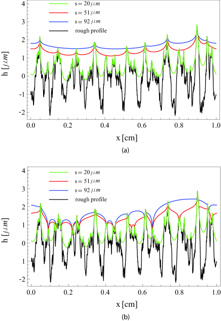
Figure 3: (Color online) The deformed shapes of the elastic body at three different separations, $s=92\mathrm{\mu m}$, $s=51\mathrm{\mu m}$, and $s=20\mathrm{\mu m}$, and the rough rigid substrate profile, for a) loading and b) unloading. The work of adhesion is $\gamma=0.01\mathrm{J/m}^{2}$, and the rigid rough substrate profile has a fractal dimension $D_{\mathrm{f}}=1.2$.

The profiles have root mean square roughness $h_{\mathrm{rms}}=\left\langle h^{2}\right\rangle^{1/2}=1\mathrm{\mu m}$. The spectral components of our profiles are given by Eq.10 and cover the wave-vector range from $q_{\min}=n_{0}q_{0}$ up to $q_{\max}=Nq_{\min}$, outside this range the PSD is zero. We have considered $\lambda=2\pi/q_{0}=6.28\mathrm{mm}$, $q_{\min}=10~{}q_{0}$ and $q_{\max}=100~{}q_{\min}$. We note that once $h_{\mathrm{rms}}$, $q_{\min}$ and $q_{\max}$ are fixed, changing the Hurst exponent (i.e. the fractal dimension of the surface) also determines a modification of the average square slope $m_{2}=$ $\left\langle h^{\prime 2}\right\rangle=\int q^{2}C_{R}\left(q\right)dq$ of the surface. For each generated rough profile (see Sec. A) the numerical calculations have been carried out for different values of the separation $s=h_{\max}-\Delta$. In Fig. 3 we show three different shapes of the deformed profile at three different values of the separation: $s=92\mathrm{\mu m}$, $s=51\mathrm{\mu m}$, and $s=20\mathrm{\mu m}$, for (a) loading and (b) unloading conditions. The work of adhesion is $\gamma=0.01\mathrm{J/m}^{2}$. The rigid rough substrate profile has a fractal dimension $D_{\mathrm{f}}=1.2$. In Fig. 3 the value $s=20\mathrm{\mu m}$ is the minimum value of separation at which the unloading process begins to take place after loading. Therefore at $s=20\mathrm{\mu m}$ the shape of the deformed profile is the same not depending on what condition (i.e. loading or unloading) is being considered. However, as the unloading proceeds further and the elastic block is moved away from the contact, the shape of the deformed profile significantly changes compared to the loading case (see $s=51,92\mathrm{\mu m}$), and is characterized by a significantly larger contact area and by the formation stretched contacts with pronounced adhesive necks Zappone-2007 . This type of behavior is peculiar of asperity adhesive contact Johnson-1971 . In fact, in presence of adhesion, asperities enter in contact when the local interfacial load is still zero, but during unloading asperities are first stretched, with the formation of adhesive neck, and then jump out of contact at negative local loads. During unloading unstable local pull-off events occur at random locations Zappone-2007 leading to pronounced differences between the loading and unloading precesses. Such different behaviors can be indirectly observed in in Fig 4, where the PSD of the rigid substrate profile (fractal dimension $D_{\mathrm{f}}=1.2$, non dimensional  penetration $\tilde{\Delta}=\Delta/h_{\max}=0.4$) has been compared to the PSD of the deformed shape of the elastic body during loading and unloading conditions, for $\gamma=0.01\mathrm{J/m}^{2}$ [Fig. 4 (b)] and $\gamma=0.04\mathrm{J/m}^{2}$ [Fig. 4 (b)].

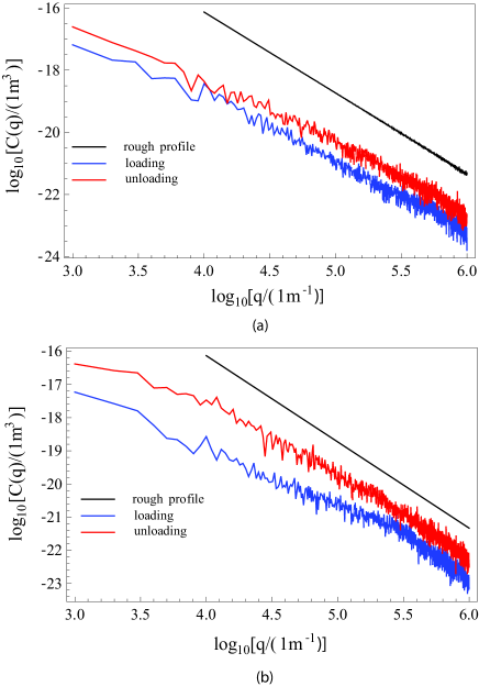
Figure 4: (Color online) The PSD of the rigid substrate profile with fractal dimension $D_{\mathrm{f}}=1.2$, compared to the PSD of the deformed shape of the elastic body at fixed non dimensional penetration $\tilde{\Delta}=\Delta/h_{\max}=0.4$, obtained for (a) $\gamma=0.01\mathrm{J/m}^{2}$ and (b) $\gamma=0.04\mathrm{J/m}^{2}$, for loading (blue curves) and unloading (red curves) conditions.

At first we remark that for large wavevectors $q$, the PSDs of the deformed profile, either in loading or unloading conditions (blue and red curves respectively), run parallel to the PSD of the rigid rough profile. This is due to the fact that, for $0.5<H<1$, full contact always occurs between the elastic block and the short wavelength corrugation of the rough rigid profile, (see Fig. 3). In fact, we can easily estimate the threshold wavelength $l_{th}$ below which full contact occurs between solid and the rigid rough substrate. To this end consider that for fractal surface the amplitude $A\left(q\right)=2\left|a\left(q\right)\right|$ of each single wavy corrugation scales as $A\left(q\right)/A\left(q_{\min}\right)\sim\left(q_{\min}/q\right)^{H}$ where $A\left(q_{\min}\right)$ is of order of the rms roughness $h_{\mathrm{rms}}$ of the substrate. Now assume that the elastic slab makes contact with the surface on a region of size $l=2\pi/q$ in this case, assuming $A\left(q\right)\ll l$, the change of elastic energy stored in the body can be shown to be $\Delta U_{el}\sim El^{2}A\left(q\right)$ whereas the change of adhesion energy upon contact is $\Delta U_{ad}\sim-\gamma l^{2}$. Therefore full contact will occur when the change of total energy $\Delta U_{tot}=\Delta U_{el}+\Delta U_{ad}$ upon contact is $\Delta U_{tot}<0$. In this case the contact will occur on a single connected region, otherwise it will be split in many different contact spots. The condition $\Delta U_{tot}<0$ gives $EA\left(q\right)<\gamma$, i.e. $A\left(q\right)<\delta=\gamma/E$ where $\delta$ is called the adhesion length. Using $A\left(q\right)/A\left(q_{\min}\right)\sim\left(q_{\min}/q\right)^{H}$ one gets $l<\left(2\pi/q_{\min}\right)\left[\delta/A\left(q_{\min}\right)\right]^{1/H}=l_{th}$. In our case we get $l_{th}\approx 2-12\mathrm{\mu m}$ depending on the value of the energy of adhesion. Therefore, during loading, at scales below this threshold value $l_{th}$ we will observe the formation of small contact where the elastic solid conforms to the rigid substrate, thus leading to the observed trend of PSD (see Fig. 4), which, indeed, runs parallel to the PSD of the rigid rough profile. At smaller spatial frequencies the contact is, instead, split in many different disconnected regions. Therefore partial contact occurs at the large scales and the slope of the PSD of the deformed profiles must necessarily differ from the one of the rigid rough profile. In Carbone-2012 the authors have shown that, under load conditions, in such smaller range of spatial frequencies and during loading conditions, the PSD of the deformed profile closely follows a power law of the type $C_{v}(q)\approx q^{(2+H)}$ in very good agreement with Persson’s theory Persson-2002 ; Persson-2005 ; Yastrebov-2012 ; Dapp-2015 ; Prodanov-2014 ; Dapp-2012 ; Dapp-2014 . However, during unloading the PSD of the deformed profile shows a different trend: (i) for large wave-vectors the unloading PSD still runs parallel to the PSD of rough profile but over a wider range of wave-vectors, (ii) at smaller spatial frequencies the slope of the PSD, instead, does not follow Persson’s predictions, as shown by the larger slope of the PSD curve compared to the loading case. This fact seems to suggest that the power law trend predicted by Persson’s theory Persson-2002 ; Persson-2005 holds true only for loading conditions. This is more evident at larger values of adhesion energy, see curve for $\gamma=0.04\mathrm{J/m}^{2}$ in Fig 4 (b). When the PSDs of the deformed profile are compared at different values of the penetration (see Fig. 5), an interesting different behavior between loading and unloading can be observed. In particular, we note that, during loading, the PSD of the deformed surface is very sensitive to the penetration value $\tilde{\Delta}$ [Fig.5 (a)], whilst this sensitivity is much less pronounced during unloading [Fig.5 (b)], at least for relatively large values of the energy of adhesion $\gamma=0.04\mathrm{J/m}^{2}$.

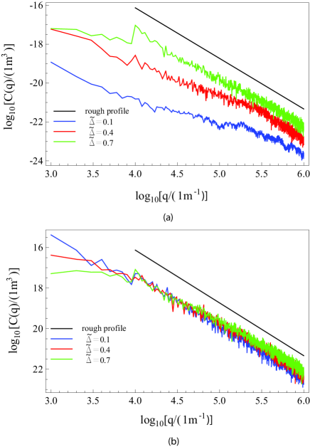
Figure 5: (Color on line) The PSD of the rigid substrate profile with fractal dimension $D_{\mathrm{f}}=1.2$, compared to the PSD of the deformed shape of the elastic body, obtained for $\gamma=0.04\mathrm{J/m}^{2}$, (a) for loading and (b) unloading conditions, for different values of the non dimensional penetration $\tilde{\Delta}=\Delta/h_{\max}$.

In Fig. 6 the normalized real contact area $A/A_{0}$ is shown, for different values of average square slope of the profile $m_{2}=\left\langle h^{\prime 2}\right\rangle$ and adhesion energy $\gamma$, as a function of the dimensionless quantity $\tilde{\sigma}/\sqrt{m_{2}}$, where $\tilde{\sigma}=2\sigma/(E^{\ast}q_{0}h_{\max})$. We have chosen to plot $A/A_{0}$ vs. $\tilde{\sigma}/\sqrt{m_{2}}$ as, for adhesiveless contacts, theories and numerical calculations [7,10,17,18,34] predict an almost linear relation between this two quantities, which is observed to be independent of the elastic properties of the material and the surface statistics.

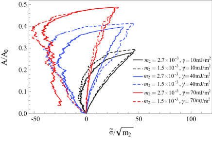
Figure 6: (Color on line) The true contact area $A/A_{0}$ as a function of the dimensionless quantity $m_{2}^{-1/2}\tilde{\sigma}$ for two different Hurst exponents $H=0.8$ ($m_{2}=2.7\times 10^{-3}$), $H=0.9$ ($m_{2}=1.5\times 10^{-3}$), and for three different values of energy of adhesion, $\gamma=0.01\mathrm{J/m}^{2}$ (black curves), $\gamma=0.04\mathrm{J/m}^{2}$ (blue curves), and $\gamma=0.07\mathrm{J/m}^{2}$ (red curves). As predicted by the theories, there is a marginal influence of the fractal dimension on the true contact area at small loads under loading conditions. The influence of $D_{f}$ becomes important during unloading. This leads to the formation of a hysteresis loading- unloading loop, which is strongly affected by the adhesion energy $\gamma.$

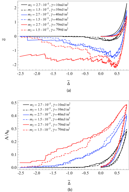
Figure 7: (Color on line) The dimensionless load $\tilde{\sigma}=2\sigma/(E^{\ast}q_{0}h_{\max})$ (a) and the quantity $A/A_{0}$ (b) as a function of the non dimensional  penetration $\tilde{\Delta}$, for two different Hurst exponents $H=0.8$ ($m_{2}=2.7\times 10^{-3}$), $H=0.9$ ($m_{2}=1.5\times 10^{-3}$), and for three different values of energy of adhesion, $\gamma=0.01\mathrm{J/m}^{2}$ (black curves), $\gamma=0.04\mathrm{J/m}^{2}$ (blue curves), and $\gamma=0.07\mathrm{J/m}^{2}$ (red curves).

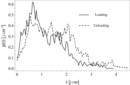
Figure 8: The normalized probability density function (PDF) $p\left(t\right)$ of the local separation $t\left(x\right)$ in the non-contact area ($t\left(x\right)>0$) for $H=0.7$, and $\gamma=0.04\mathrm{J/m}^{2}$, $\tilde{\Delta}=0.7$ for (a) loading and (b) unloading conditions.

However, in our case, this linearity is not observed, especially when the two surfaces are moved apart (unloading). More importantly, given the same applied load, the contact area during unloading is much larger than during loading, thus leading to strong hysteresis. This is even more clear in Figure 7 (a) where the dimensionless load $\tilde{\sigma}$ is plotted vs. the non dimensional penetration $\tilde{\Delta}$. Interestingly, being the solid perfectly elastic, such a hysteretic energy dissipation must be related to contact phenomena occurring at the interface. In fact we can propose two different mechanisms leading to energy dissipation: (i) the first occurring at small scales, i.e. for wavelength $l<l_{th}$, which we refer to as the Small-Scale-Hysteresis (SSH); (ii) the second at large scales, i.e. for $l>l_{th}$, which we refer to as the Large-Scale-Hysteresis (LSH). To understand the origin of the SSH, let us recall that at small scales the solid conforms to the rigid substrate. Thus, each single contact is actually represented by a compact interval. In such a case Guduru and his collaborators have shown that, already a moderate roughness strongly modifies the original JKR curve providing it with a non-monotonic behavior Guduru-2007 ; Guduru-2007BIS . This, in turn, causes the unloading process to be characterized by many crack propagation jumps, with the interface separating in alternating stable and unstable segments. Each unstable segments dissipates energy leading to an increase of the total work during unloading and, hence, to energy dissipation. This unstable behavior has been used in Ref. Kesari-2010 to justify the hysteresis observed in JKR experiments with AFM tips.

The origin os LSH is instead different. In fact, as noted so far, when the surface is observed at large scales the contact is constituted by a set of disconnected small contact regions, where the short wavelength corrugation is apparently smoothed out. The contact interface, then, appears as the contact between as certain number of randomly located smooth asperities, each of one obeying the JKR adhesion laws. In such conditions Israelachivili and his group Zappone-2007 proposed a very simple picture to explain the occurrence of hysteresis. As noted so far, this is indeed due to the local stretching and consequent JKR pull-off of asperities during unloading Zappone-2007 .

It is noteworthy to observe that increasing the energy of adhesion $\gamma$ leads to a strong increase of hysteresis loop [see Fig. 7 (a)]. The origin of this behavior is twofold as increasing $\gamma$ necessarily leads to: (i) an increase of number of contact patches, and (ii) to an increase of the size of each single contact patch. This, in turn, determines an enhancement of SSH and LSH phenomena, i.e. to a large increment of energy dissipation during the loading-unloading loop. Figure 7 (b) shows the reduced real contact area $A/A_{0}$ as a function of the dimensionless penetration $\tilde{\Delta}$ for two different Hurst exponents $H=0.8$ ($m_{2}=2.7\times 10^{-3}$), $H=0.9$ ($m_{2}=1.5\times 10^{-3}$), and for three different values of energy of adhesion, $\gamma=0.01\mathrm{J/m}^{2}$ (black curves), $\gamma=0.04\mathrm{J/m}^{2}$ (blue curves), and $\gamma=0.07\mathrm{J/m}^{2}$ (red curves).

	$\gamma=0.01\mathrm{J/m}^{2}$	$0.04\mathrm{J/m}^{2}$	$0.07\mathrm{J/m}^{2}$
$m_{2}=5.1\times 10^{-3}$	-	26.6	42.83
$2.7\times 10^{-3}$	3.44	19.36	49.25
$1.5\times 10^{-3}$	2.59	17.91	28.15

Tab.1 - The dimensionless energy loss.

An estimation of the dimensionless energy loss during the entire loading-unloading cycle, for different values of the average square slope of the profile, is given in Table 1. In particular no general trend can be inferred. Results, instead, may suggest a non monotonic dependence of the dissipated energy on $m_{2}$. This is, infact, what we expect. Simple dimensional argument show indeed that the density $D_{\mathrm{sum}}$ of the substrate asperities increases as $D_{\mathrm{sum}}\sim\sqrt{m_{4}/m_{2}}$ where $m_{4}=\left\langle h^{\prime\prime 2}\right\rangle=\int q^{4}C_{R}\left(q\right)dq$ is the average square curvature of the rough profile. Thus, considering that $m_{4}$ increases with $m_{2}$ faster than $m_{2}$, it follows that the number of asperities per unit length grows as $m_{2}$ is increased. Therefore, for moderate values of the average square slope, increasing $m_{2}$ should lead, by following the mechanism proposed in Ref. Guduru-2007 ; Guduru-2007BIS to an enhancement of the SSH hysteresis in each contact spot, and to and increment of the number of contact spots, thus increasing the number of LSH pull-off events. Hence, for small $m_{2}$, increasing $m_{2}$ should necessarily causes an increase of hysteresis.

However, for sufficiently large values of $m_{2}$, the number of contact spots as well as the contact area in each contact spot must strongly diminish (given the same value of $\gamma$). This follows from the fact that, as shown above, full contact between the elastic solid and the rigid substrate on the length-scale $l=2\pi/q$, occurs when the amplitude $A\left(q\right)$ of the spectral components satisfies the relation $A\left(q\right)<\delta$, that is to say $m_{2}\left(q\right)<\left(\delta/l\right)^{2}$, where $m_{2}\left(q\right)\approx\left[A\left(q\right)/l\right]^{2}$ is the average square slope of $q$-component of the rigid rough profile. Therefore, increasing $m_{2}$ will cause full contact conditions to be established at continuously decreasing lengthscales. This will strongly reduce the contact area in each contact spots, will reduce the force needed to detach the elastic body from the rigid substrate and in the end strongly diminish the adhesion hysteresis, in agreement with experimental observations in AFM contacts in Ref. Kesari-2010 .

Fig. 8 shows the normalized conditional probability density function (PDF) $p\left(t\right)$ of the interfacial separation $t\left(x\right)=v\left(x\right)-h\left(x\right)+s$ in the non contact area (where $t>0$). $t\left(x\right)$ plays a crucial rule in many practical applications (e.g. mixed lubrication, lip seals, static seals). The PDF has been calculated for $H=0.7$, and $\gamma=0.04\mathrm{J/m}^{2}$, in (a) loading and (b) unloading conditions. The trend of the calculated $p\left(t\right)$ in the loading and unloading conditions slightly differs in Figure 8, since during unloading (see Fig. 3), the shape of the deformed profiles changes leading to higher interfacial separations $t\left(x\right)$ compared to the loading case. This explains the trend of $p\left(t\right)$ in Figure 8 for the unloading case: the $p\left(t\right)$ is, in fact, slightly shifted towards higher values of separation $t\left(x\right)$ compared to the loading case.

IV Conclusions

In this paper we have studied the adhesive contact between a rubber block and a rigid randomly rough profile during loading and unloading conditions. The roughness has been considered to be a self-affine fractal on a limited range of wave-vectors. Calculations have been carried out for each profile by means of an ad hoc numerical code previously developed by the authors. The calculated data have been statistically averaged, and the influence of profile average slope and energy of adhesion on loading-unloading contact behavior has been investigated. We have shown that the combination of adhesion and roughness leads to the appearance of hysteresis cycle and, hence, to energy dissipation. We physically justify the observed behavior by considering two sources of energy dissipation one occurring at small scales and the second at large scales. We have numerically quantified the energy loss depending on the average slope of roughness and on the energy of adhesion and discuss it in terms of surface statistical properties.

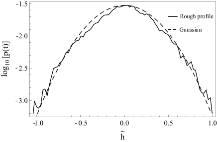
Figure 9: The averaged dimensionless height probability density function $p\left(t\right)$ of 10 rigid rough profiles. $\tilde{h}\left(x\right)=h\left(x\right)/h_{\max}$. Calculations are shown for $H=0.8$. Because of the enhanced ergodicity, the trend of the calculated probability density function $p\left(t\right)$ (solid line) follows pretty well a Gaussian random distribution (dashed line).

Appendix A Rough profile generation

In our numerical calculations we have utilized a periodic profile with wavectors in the range $q_{0}<q<q_{\max}$. In particular, the non-vanishing spectral components of our profiles are given by Eq. 10 in the range from $q_{\min}=n_{0}q_{0}<q<q_{\max}=Nq_{\min}$. Out of this range the PSD is zero. This choice is necessary in order to improve the ergodicity of the process. For the numerical generation of a profile, it is necessary to determine the amplitudes $\left|a_{m}\right|$ and the phases $\phi_{m}$ of the terms $a_{m}=\left|a_{m}\right|e^{i\phi_{m}}$ [see Eq. (1)]. It can be shown that in order to satisfy the translational invariance of the profile statistical properties (which implies that the autocorrelation function satisfies the relation $\left\langle h\left(x^{\prime}\right)h\left(x^{\prime}+x\right)\right\rangle=\left\langle h\left(0\right)h\left(x\right)\right\rangle$), it is enough to assume that the random phases $\phi_{m}$ are uniformly distributed on the interval $\left[-\pi,\pi\right[$. This also guarantees that the process is Gaussian. Now moving from Eq. (1) the PSD is

$$C\left(q\right)={\displaystyle\sum\limits_{m=-\infty}^{+\infty}}\left\langle\left|a_{m}\right|^{2}\right\rangle\delta\left(q-mq_{0}\right)$$ (11)

from which it follows

$$C\left(mq_{0}\right)=\left\langle\left|a_{m}\right|^{2}\right\rangle\delta\left(0\right)$$ (12)

If we assume self-affine fractal profile [see Eq. (10)] one obtains

$$\left\langle\left|a_{m}\right|^{2}\right\rangle=\left\langle\left|a_{1}\right|^{2}\right\rangle m^{-\left(2H+1\right)}$$ (13)

Hence, the quantity $\left\langle\left|a_{m}\right|^{2}\right\rangle$ can be determined once known $\left\langle\left|a_{1}\right|^{2}\right\rangle$ and the Hurst exponent of the surface. However to completely characterize the rough profile we still need the probability distribution of the amplitudes $\left|a_{m}\right|$. There are several choices, however the simplest assumption, as suggested by Persson et al. in Ref. Persson-2005 , is that the probability density function of $\left|a_{m}\right|$ is just a Dirac’s delta function centered at $\left\langle\left|a_{m}\right|^{2}\right\rangle^{1/2}$, i.e.

$$p\left(\left|a_{m}\right|\right)=\delta\left(\left|a_{m}\right|-\left\langle\left|a_{m}\right|^{2}\right\rangle^{1/2}\right)$$ (14)

Fig. 9 shows the averaged probability density function $p\left(t\right)$ of 10 profile dimensionless roughness heights $\tilde{h}\left(x\right)=h\left(x\right)/h_{\max}$. The Hurst exponent is $H=0.8$. Thanks to the improved ergodicity of the numerically generated rough profile, the trend of the calculated probability density function $p\left(t\right)$ (solid line) follows closely a Gaussian distribution (dashed line).

References

- (1) B.N.J. Persson and C. Yang, J. Phys. Condens. Matter 20, 315011 (2008).
- (2) B. Lorenz and B.N.J. Persson, Eur. Phys. J. E 31, 159-167 (2010).
- (3) M. Scaraggi, G. Carbone, B.N.J. Persson, D. Dini, Soft Matter 7 (21), 10395-10406 (2011).
- (4) M. Scaraggi, G. Carbone, and D. Dini. Tribol. Lett. 4 (2), 169-174 (2011).
- (5) G. Carbone and L. Mangialardi, J. Mech. Phys. Solids 56, 684-706 (2008).
- (6) Y.P. Zhao, L. S. Wang and T. X. Yu. J. Adhes. Sci. Technol. 17, 519-546 (2003).
- (7) G. Carbone and C. Putignano, J. Mech. Phys. Solids, vol. 61, pp. 1822-1834 (2013).
- (8) Geim, A.K., Dubonos, S.V., Gricorieva, I.V., Novoselov, K.S., Zhukov, A.A., Shapoval, S.Yu., Nat. Mater. 2, 461–463 (2003).
- (9) Carbone G., Pierro E., Gorb S., Soft Matter 7 (12), 5545-5552 (2011).
- (10) Carbone G., Pierro E., J Adhes Sci Technol 26 (22), 2555-2570 (2012).
- (11) Bottiglione, F., Carbone, G., Mangialardi, L., Mantriota, G., J. Appl. Phys. 106, 104902 (2009).
- (12) W. B. Dapp, A. Lücke, B.N.J. Persson and M. H. Müser, PRL 108, 244301 (2012).
- (13) Pickering J. P., Van Der Meer D. W., Vancso G. J., J Adhes Sci Technol, 15 (12), 1429-1441 (2001).
- (14) Y. Chen, C. Helm, J. Israelachvili, J. Phys. Chem., 95, pp. 10736 (1991).
- (15) Maeda N., Chen N., Tirrell M., Israelachvili J. N., Science, 297 (5580), 379-382, (2002).
- (16) K. N. G. Fuller and D. Tabor, Proc. R. Soc. Lond. A 345, 327-342 (1975).
- (17) Pastewka L. and Robbins M. O., Proc. Natl. Acad. Sci. USA, vol. 111 no. 9, 3298–3303 (2014).
- (18) Hyun S., Pei L., Molinari J.-F., and Robbins M. O., Phys. Rev. E, 09/2004; 70(2 Pt 2)-026117 (2004).
- (19) B. Luan, Robbins M. O., Tribol Lett 36,1–16 (2009).
- (20) Jackson R. L. and Green I., Tribol T, 54, 300-314 (2011).
- (21) Medina S., Dini D., Int J Solids Struct, 51 2620–2632 (2014).
- (22) Medina S., Nowell D., Dini D., Tribol Lett 49, 103–115 (2013).
- (23) Sellgren U., Björklund S., Andersson S., Wear 254, 1180–1188 (2003).
- (24) Eid H., Adams G. G., McGruer N. E., Fortini A., Buldyrev S., Srolovitz D., Tribol T, 54 (6), 920-928, (2011).
- (25) Kadin Y., Kligerman Y., Etsion I., J Mech Phys Solids 54, 2652–2674 (2006).
- (26) Li L., Song W. , Xu M., Ovcharenko A. , Zhang G., Comput. Mater. Sci. 98 105–111(2015).
- (27) Kadin Y., Kligerman Y., Etsion I., J. Colloid Interface Sci. 321, 242–250 (2008).
- (28) Tirrell M., Langmuir, 12 (19), 4548-4551 (1996).
- (29) Greenwood J. A., Johnson K. L., Philos Mag A, 43 (3), 697-711 (1981).
- (30) Guduru P.R., J Mech Phys Solids, 55 (3), 445-472 (2007).
- (31) Guduru P.R., Bull C., J Mech Phys Solids, 55 (3), 473-488 (2007).
- (32) Zappone B., Rosenberg K. J., Israelachvili J., Tribol Lett, 26 (3), 191-201 (2007).
- (33) Kesari H., Doll J. C., Pruitt B. L., Cai W., Lew A. J., Phil Mag Lett, 90 (12), 891-902 (2010).
- (34) G. Carbone, M. Scaraggi and U. Tartaglino, European Phys. J. E 30, 65–74 (2009).
- (35) K. L. Johnson, K. Kendall, and A. D. Roberts., Proc. Roy. Soc. London A 324, 301–313 (1971).
- (36) B.N.J. Persson. Eur. Phys. J. E 8, 385 (2002).
- (37) Persson B. N. J., Albohr O., Tartaglino U., Volokitin A. I., Tosatti E., J. Phys.: Condens. Matter 17 R1–R62 (2005).
- (38) Yastrebov V. A., Anciaux G., and Molinari J. F., Phys. Rev. E 86, 035601(R) (2012).
- (39) Dapp W. B. and Müser M. H., EPL, 109 44001(2015).
- (40) Prodanov N., Dapp W. B., Müser M. H., Tribol Lett 53, 433–448(2014).
- (41) Dapp W. B., Prodanov N.,Müser M. H., Phys.: Condens. Matter, 26-355002 (2014).