Diagnose Physical Conditions Near the Flare Energy-release Sites from Observations of Solar Microwave Type III Bursts

Abstract

In the physics of solar flares, it is crucial to diagnose the physical conditions near the flare energy-release sites. However, so far it is unclear how do diagnose these physical conditions. Solar microwave type III burst is believed to be a sensitive signature of the primary energy release and electron accelerations in solar flares. This work takes into account the effect of magnetic field on the plasma density and developed s set of formulas which can be used to estimate the plasma density, temperature, magnetic field near the magnetic reconnection site and particle acceleration region, and the velocity and energy of electron beams. We applied these formulas to three groups of microwave type III pairs in a X-class flare, and obtained some reasonable and interesting results. This method can be applied to other microwave type III bursts to diagnose the physical conditions of source regions, and provide some basic information to understand the intrinsic nature and fundamental processes occurring near the flare energy-release sites.

1 Introduction

In solar flares, the energetic particles play a prominent role in energy release, transmission, conversion, and emission propagation. Estimation shows that energetic particles may carry about 10 - 50% of the total energy released in a typical X-class flare (Lin & Hudson, 1976). However, so far, there are many unresolved problems on the solar energetic particles, especially the energetic electrons, such as where is the site of electron acceleration? What is the exact mechanism of particle acceleration? How fast of the energetic electron beams flying away from its source region? It is necessary to measure clearly the physical conditions around the source region for answering the above questions. These conditions include plasma density, temperature, magnetic field, and energy of particle beams (Zharkova et al. 2008).

Solar radio type III burst is believed to be a sensitive signature of the energetic electron beams generated and propagated in the corona. It is interpreted as caused by energetic electron beam streaming through the background plasma at a speed of about 0.1 - 0.9$\mathrm{c}$ ($\mathrm{c}$ is the light speed) propagating away from the acceleration site (e.g., Lin & Hudson 1971, Lin et al. 1981, and a recent review in Reid & Ratcliffe 2014). In meter or longer wavelengths, solar radio type III bursts are regarded to be generated by energetic electron beams propagating upward in open magnetic field configurations, their frequency drift rates are negative and be called normal type III bursts, their emission source may locate above the flare energy-release site. But in decimeter- or shorter wavelengths, the frequency drift rates of type III bursts are always positive, we called them as microwave type III bursts which regarded to be produced by the electron beams propagating downward, their emission source may locate below the flare energy-release site. Occasionally there will be observed microwave type III burst pairs, which are composed of normal type III branches with negative frequency drift rates and reverse-sloped (RS) type III branches with positive frequency drift rates simultaneously. Microwave type III pairs are explained as produced by bi-directional electron beams and their source regions are very close to the flare energy-release site where the magnetic reconnection and particle acceleration take place. Therefore, microwave type III bursts, including the microwave type III pairs, are the most important tool to diagnose the physical conditions around the flare energy-release sites. It may provide the most important information for understanding the flare triggering mechanism and particle acceleration.

The short lifetimes and very high brightness temperatures of microwave type III bursts indicate that the emission should be coherent processes. The first coherent mechanism is electron cyclotron maser emission (ECM, Melrose & Dulk 1982, Tang et al. 2012) which requires a strong background magnetic field: $f_{ce}>f_{pe}$. $f_{ce}$ is electron gyro-frequency and $f_{pe}$ is plasma frequency. As for the microwave type III bursts, the required magnetic fields should be $B>1000$ G, too strong to occur in solar corona. The second coherent mechanism is plasma emission (PE, Zheleznyakov & Zlotnik 1975) which is generated from the coupling of two excited plasma waves at frequency of 2$f_{pe}$ (second harmonic PE), or the coupling of an excited plasma wave and a low-frequency electrostatic wave at frequency of about $f_{pe}$ (fundamental PE). As PE has no strong magnetic field constraints, it is much easy to be the favorite mechanism of type III bursts.

In PE mechanism, the emission frequency can be expressed

$$f\approx 9sn_{e}^{\frac{1}{2}}.$$ (1)

The units of $f$ and $n_{e}$ are Hz and m s^-3, respectively. $s$ is the harmonic number, $s=1$ is the fundamental PE while $s=2$ is the second harmonic PE. Generally, the fundamental PE has strong circular polarization, while the second harmonic PE always has relatively weak circular polarization.

The frequency drift rate is the most prominent observed parameter of microwave type III bursts, which is connected to many physical conditions in the source region. From Equation (1), we derived:

$$D=\frac{df}{dt}=\frac{f}{2}(\frac{\partial n_{e}}{n_{e}\partial t}+\frac{\partial n_{e}}{n_{e}\partial l}\cdot\frac{\partial l}{\partial t})=\frac{f}{2}(\frac{1}{t_{n}}+\frac{v_{b}}{H_{n}})$$ (2)

The relative frequency drift rate is expressed,

$$\bar{D}=\frac{df}{fdt}=\frac{1}{2t_{n}}+\frac{v_{b}}{2H_{n}}$$ (3)

$H_{n}=\frac{n_{e}}{\partial n_{e}/\partial l}$ is the plasma density scale length along the electron beams. $H_{n}>0$ or $H_{n}<0$ means the density increasing or decreasing along the electron beam. $t_{n}=\frac{n_{e}}{\partial n_{e}/\partial t}$ is the plasma density scale time. $t_{n}>0$ or $t_{n}<0$ means the density increasing or decreasing with respect to time. $\frac{\partial l}{\partial t}=v_{b}$ is the velocity of electron beams.

Equation (2) and (3) shows that frequency drift rate is composed of two parts. The first part is related to the temporal variation of plasma density, and the second part is related to the spatial variation of plasma density which is caused by plasma density gradient and the motion of electron beams.

In flare impulsive phase, fast magnetic reconnection may produce plasmas inflow into the reconnecting region and result in plasma density increasing, $t_{n}>0$. In postflare phase, magnetic reconnection becomes very weak, and there is no obviously variation of the plasma density, $t_{n}\rightarrow\infty$ and the first term of Equation(2) and (3) can be neglected.

$H_{n}$ depends on plasma density distributions (Dulk 1985). So far, the most common plasma density models of the quiet solar atmosphere are Baumbach-Allen model (Allen 1947) and Newkirk model (Newkirk, 1967). When applying these models to the active region, it is always necessary to multiply by a number from 3 to 50. Naturally, this method has a big uncertainty. By using the broadband radio spectral observations of the solar eclipse, Tan et al. (2009) obtained an improved semi-empirical model of the coronal plasma density. However, the above models are expressed as functions of height from the solar surface. It is difficult to apply them to a microwave type III burst at a certain frequency when the height of the source region is not known. Under the assumption of solar static and barometric atmosphere, $H_{n}$ can be estimated as $H_{n}=-\frac{k_{B}T}{m_{0}g}$ (Benz et al. 1983). $k_{B}$ is the Boltzmann constant, $g$ the solar gravitational acceleration ($\sim$274 ms^-2 near the solar surface), and $m_{0}$ the average mass of ions in the solar chromosphere and corona. The minus sign indicates the density decreasing with respect to the height. The barometric model is only valid in the quiet corona and not appropriate for the type III-emitting source region that cannot be in hydrodynamic equilibrium because of the substantial heating and plasma flows. The generated microwaves are subject to free-free absorption when they propagates in the ambient plasma, they will be strongly absorbed. Assuming the plasma is isothermal and barometric, then the density scale length corresponding to the optical depth unity is about, $H_{n}\approx 6.67\times 10^{14}\frac{T^{3/2}}{f^{2}}$ (m) for the fundamental emission, and $H_{n}\approx 1.07\times 10^{16}\frac{T^{3/2}}{f^{2}}$ (m) for the harmonic emission (Dulk 1985, Stahli & Benz 1987). But when applying this expression to estimate the electron beam velocity, we find $v_{b}>1.0$ c in some events, and $v_{b}<0.1$ c in other events. These results are unreasonable. Aschwanden & Benz (1995) proposed a combined model by assuming a power-law function in the lower corona and an exponential function in the upper corona. However, as the above models have not considered the effect of magnetic fields, they can not reflect the relationship between the physical conditions and the properties of the microwave type III bursts.

This work plans to propose a new method to diagnose the physical conditions around the flaring energy-release sites from observations of solar microwave type III bursts. Section 2 introduces the main observable parameters of microwave type III bursts. In Section 3, we derived a new expression of the plasma density scale length ($H_{n}$) from the full MHD equation which contains magnetic pressure force. On this basis, we proposed a set of formulas to estimate the plasma density, temperature, magnetic field around the primary source region of solar flares, and the velocity and energy of the energetic electron beams. In Section 4, we apply the above method to diagnose the source region of three groups of microwave type III bursts pair in the postflare phase of a X-class flare. Finally, conclusions are summarized in Section 5.

2 Observing Parameters of Microwave Type III Bursts

Recently, there are many solar radio spectrometers having been operated at frequency of microwave range with high frequency and time resolutions. For example, the Chinese Solar Broadband Radio Spectrometers at Huairou (SBRS) operates with dual circular polarization (left- and right-handed circular polarization) in the frequency range of 1.10 – 2.06 GHz, 2.60 – 3.80 GHz, and 5.20 – 7.60 GHz, their cadence is 5 – 8 ms, and the frequency resolution is 4 – 20 MHz (Fu et al. 1995, 2004, Yan et al. 2002). The Ondřejov radiospectrograph in the Czech Republic (ORSC) operates at frequencies of 0.80-5.00 GHz, its cadence is 10 ms and the frequency resolution is 5-12 MHz (Jiřička et al. 1993).

From the observations of the microwave type III bursts, we can derived several observable parameters:

(1) Start frequency ($f_{st}$), defined as the frequency at the start point of the microwave type III burst with emission intensity exceeding the background significantly.

(2) Burst lifetime ($\tau$), defined as the time difference between the start and end of an individual type III burst.

(3) Central frequency ($f_{0}$), defined as the frequency at the midpoint of type III burst.

(4) Frequency drift rates ($D=\frac{df}{dt}$), defined as slopes of type III burst on the spectrograms. $f$ is the frequency at the ridge crest along the type III burst at different time. Generally, frequency drift rate can be derived by using cross-correlation analysis at each two adjacent frequency channels.

(5) The relative frequency drift rates ($\bar{D}$), defined as $\bar{D}=\frac{df}{fdt}\approx\frac{D}{f_{0}}$.

3 Diagnostics to the Flare Energy-release Site

In order to understand the process of microwave type III bursts, we construct a physical scenario to demonstrate roughly the possible processes of magnetic reconnection, particle accelerations and propagations associated to microwave type III bursts in solar flares (Fig. 1). Here magnetic reconnection may take place in a cusp configuration above and very close to the top of flaring loop similar as the Masuda-like flare (Masuda et al. 1994, etc.), or in the current sheet above and beyond flare loops triggered by the tearing-mode instability (Kliem et al. 2000, etc). In some flares the reconnections are more dominated in cusp configuration and in other flares in current sheets. Electrons are accelerated in the reconnection site (source region), propagate upward or downward, and produce normal or RS type III bursts.

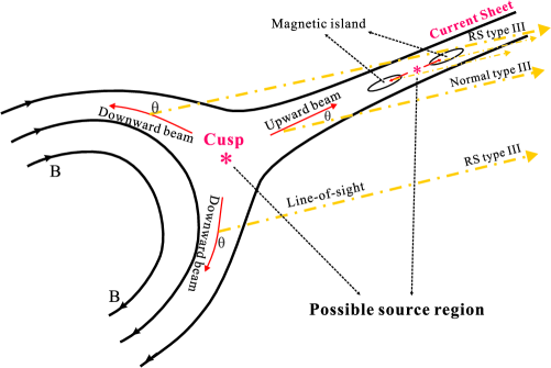
Figure 1: Schematic diagram of the formation of radio type III burst pairs. Red arrows indicate the path of the energetic electron beams, and the yellow arrows indicate the emission direction.

In this section, a new diagnostic method can be derived in framework of the above physical scenarios.

3.1 Constraints of the Emission Process

As we mentioned in Section 1, the most possible emission mechanism of microwave type III bursts is the plasma emission. There are some constraints to this mechanism for a certain microwave type III bursts (Cairns & Melrose 1985, Robinson & Benz 2000):

(1) Magnetic field. $f_{ce}<f_{pe}$ and $f>f_{pe}$ requires a relatively weak magnetic field $B<3.57\times 10^{-7}f$ (G). Here, the unit of $f$ is Hz. For example, the magnetic field must be $B<1070$ G at frequency of 3 GHz. For most cases, this condition is easy to agree.

(2) Emission Frequency. PE mechanism is a three-wave interaction process, which must satisfy frequency condition $f_{T}=f_{L}+f_{3}$. Here $T$, $L$, and $3$ represent the transverse radiation, Langmuir wave, and the third wave, respectively. When the third wave is an ion-sound wave it will produce fundamental emission; and a second harmonic emission will produce when the third wave is a secondary Langmuir wave.

(3) Beam direction. The three-wave interaction requires wave-vector conservation $k_{T}=k_{L}+k_{3}$. Here, $k_{L}$ is almost at the electron beams direction, while $k_{3}$ have broad distributions. As for the fundamental emission, $k_{3}$ represents an ion-sound wave and $k_{3}\ll k_{L}$, the emission ($k_{T}$) is approximately at the same direction of electron beams. As for the second harmonic emission, $k_{3}$ represents a secondary Langmuir wave, $k_{T}$ may obviously deviate from the electron beams.

(4) Beam velocity. Not all electron beams can generate Langmuir waves to produce a certain type III burst, actually only the beam with positive derivative distribution function in velocity space can produce Langmuir waves by bump-in-tail instability. The positive derivative distribution function must be formed on the total distribution function (background Maxwellian distribution + beam distribution), and this means that the velocity of electron beam must exceed a lower limit which is above the thermal velocity of the background Maxwellian distribution, especially for the low density beams:

$$v_{b}>3.2\times 10^{2}(n_{e}\tau)^{1/3}=v_{L}$$ (4)

The above equation is derived from the relationship $\tau<t_{d}$. $\tau$ is the observed lifetime of microwave type III burst. $t_{d}=3.1\times 10^{-8}\frac{v_{b}^{3}}{n_{e}}$ is the collisional deflected time of electron beams, here the units of $v_{b}$ and $n_{e}$ are $m\cdot s^{-1}$ and $m^{-3}$, respectively (Benz et al. 1992). The lower limit indicates that low energy electron beam will be dissipated in dense plasma and cannot produce coherent emission.

At the same time, the dispersion relation of PE emission also requires an upper velocity limit:

$$v_{b}<\frac{3}{2}\sqrt{\frac{m_{i}}{\gamma m_{e}}}V_{0}=v_{H}$$ (5)

Here $\gamma=1+3\frac{T_{i}}{T_{e}}\approx 2$, $V_{0}$ is the electron thermal velocity, $v_{H}$ is a critical velocity ($\approx 40-50V_{0}$), $m_{e}$ and $m_{i}$ are electron and mean ion mass, $T_{i}$ and $T_{e}$ are ion and electron temperatures, respectively. The upper velocity limit indicates that very high energy electron beam will not produce plasma emission when propagating in cold plasmas. In very hot plasma, for example, when $T_{e}\approx 3\times 10^{6}$ K, $v_{H}\approx c$. At such case, the upper limit is the light speed. The full velocity constraint for PE-emitting electron beam is $v_{L}<v_{b}<v_{H}$. This constraint is very meaningful for estimating the magnetic field near source regions. We will demonstrate it in Section 3.5.

3.2 Plasma Density and Temperature

The emission of microwave type III burst generates close to the flare primary source region. By using the observed start frequency ($f_{st}$), the plasma density near the start site of the electron beam can be obtained from Equation (1):

$$n_{st}=f_{st}^{2}/81s^{2},(m^{-3}).$$ (6)

The temperature can be derived approximately from the ratio of soft X-ray (SXR) intensities at two energy band observed by GOES satellite after subtracting the background by using the Solar Software (Thomas et al. 1985). Applying this method, we obtained the temperature profiles in each flare. From these profiles, we can get the temperature at the time of microwave type III burst. However, it is important to note that the above temperature is only related to the hot flaring loops which is possible different from the real source region of microwave type III bursts.

3.3 Frequency Drift Rates

Equation (2) and (3) indicate that the frequency drift rate of microwave type III burst is composed of two parts. When the temporal change is neglected, the frequency drift rate only depends on the ratio between the beam velocity ($v_{b}$) and the density scale length ($H_{n}$) along the path of source (Benz et al. 1983). Therefore, $H_{n}$ is a key factor to estimate the beam velocity from frequency drift rate of microwave type III bursts. However, as we mentioned in Section 1, there is a considerable uncertainty to determine the value of $H_{n}$ by using the existing methods. All the above methods have not considered the effect of magnetic fields on the plasma density and its distribution.

Actually, magnetic field is a key factor in flare energy-release sites, which compresses and confines plasma, and dominates the plasma density and its distribution. As a consequence, $H_{n}$ is also dominated by the magnetic field. In this section, we try to deduce an expression of $H_{n}$ from a full MHD equation including plasma thermal pressure force ($\nabla p$), Lorentz force ($\vec{j}\times\vec{B}$), and gravitational force ($\rho\vec{g}$),

$$\frac{d(\rho\vec{v})}{dt}=-\nabla p+\vec{j}\times\vec{B}+\rho\vec{g}$$ (7)

In quasi-equilibrium, $\frac{d(\rho\vec{v})}{dt}\sim 0$, $\nabla p\sim\frac{n_{e}k_{B}T}{H_{n}}$. The Lorentz force can be decomposed into:

$$\vec{j}\times\vec{B}=\frac{1}{\mu_{0}}(\vec{B}\cdot\nabla)\vec{B}-\nabla(\frac{B^{2}}{2\mu_{0}})$$ (8)

Furthermore, the first and second terms in the right side can be expressed respectively as,

$$\frac{1}{\mu_{0}}(\vec{B}\cdot\nabla)\vec{B}=\frac{d}{ds}(\frac{B^{2}}{2\mu_{0}})\vec{s}+\frac{B^{2}}{\mu_{0}R_{c}}\vec{s}$$ (9)

$$-\nabla(\frac{B^{2}}{2\mu_{0}})=-\frac{d}{ds}(\frac{B^{2}}{2\mu_{0}})\vec{s}-\nabla_{\perp}(\frac{B^{2}}{2\mu_{0}})\vec{n}.$$ (10)

Here, the unit vector $\vec{s}$ is along the magnetic field line, and $\vec{n}$ is normal to the magnetic field lines, and $R_{c}$ is the curvature radius of the magnetic field lines.

Substituting Equation (9) and (10) into (8), then, we have

$$\vec{j}\times\vec{B}=\frac{B^{2}}{\mu_{0}R_{c}}\vec{s}-\nabla_{\perp}(\frac{B^{2}}{2\mu_{0}})\vec{n}.$$ (11)

The first term of Equation (11) is the magnetic tension force which is acting along the direction of magnetic field, has resultant effect only when the magnetic field line is curved. The second term is the magnetic pressure force which is acting at the direction perpendicular to the magnetic field lines, and this force will compress and confine the plasmas (Priest 2014). Any changes of the magnetic field strength will lead to a corresponding variation in plasma density. Therefore plasma density is dominated by the magnetic field. In the actual condition near the flare energy-release site, there also has magnetic gradient between different points along the magnetic field lines, and this will lead to a density gradient between the different points along the magnetic field. Substituting Equation (11) into Equation (7), we have,

$$\frac{d(\rho\vec{v})}{dt}=-[\nabla_{\parallel}P-\frac{B^{2}}{\mu_{0}R_{c}}+m_{0}n_{st}g\cos\theta]\textbf{s}-[\nabla_{\perp}P+\nabla_{\perp}(\frac{B^{2}}{2\mu_{0}})-m_{0}n_{st}g\sin\theta]\textbf{n}$$ (12)

Here, the plasma thermal pressure $P=n_{st}k_{B}T_{e}$. Fig. 1 indicates that the electron beams are mainly propagating along the magnetic field lines, we may let the longitudinal component approached zero, $\nabla_{\parallel}(n_{st}k_{B}T_{e})\approx\frac{n_{st}k_{B}T_{e}}{H_{n}}$. $H_{n}$ is the plasma density scale length along the magnetic field lines,

$$H_{n}=\frac{k_{B}T}{\frac{B^{2}}{n_{st}\mu_{0}R_{c}}-m_{0}g\cos\theta}.$$ (13)

In barometric atmosphere model, $\vec{j}\times\vec{B}\rightarrow 0$, we can derive the barometric density scale length $H_{n}=-\frac{k_{B}T}{m_{0}g}$ directly from Equation (7). Actually, when the magnetic field is very weak $B\rightarrow 0$, or in a homogeneous magnetic field $R_{c}\rightarrow\infty$, the first term of the denominator vanishes, and assume $\theta\rightarrow 0$, Equation (13) will degenerate to be the barometric format. For example, the radio type III burst at meter or longer wavelength is generally explained as the propagation of electron beam in the open magnetic field in upper corona where the magnetic field is very weak and the curvature radius of the magnetic field lines is very longer, the barometric model can explain the main properties of radio type III bursts very well.

As for the microwave type III burst, its source region is very close to the acceleration regions and very low. Here the magnetic field is relatively strong, for example, with a possible typical values of parameters, $B=$ 20 G, $n_{st}=10^{10}$ cm^-3, and $R_{c}=10^{4}$ km, then $\frac{B^{2}}{n_{st}\mu_{0}R_{c}}\sim$ 100 $m_{0}g$, that means it is very easy to have the relation $\frac{B^{2}}{n_{st}\mu_{0}R_{c}}\gg m_{0}g$. This fact implies that magnetic field does play a dominant role to the plasma density scale length near acceleration regions. Then, Equation (13) can be approximated,

$$H_{n}\approx\frac{\mu_{0}n_{st}k_{B}T}{B^{2}}R_{c}=\frac{1}{2}\beta_{p}\cdot R_{c}.$$ (14)

$\beta_{p}=\frac{n_{st}k_{B}T}{B^{2}/(2\mu_{0})}$ is the plasma beta defined as the ratio between the plasma thermal pressure and the magnetic pressure. Equation (14) indicates that the plasma density scale length ($H_{n}$) can be replaced by measuring the configuration of the magnetic field ($R_{c}$).

3.4 Electron Beams

The electron beams associated to microwave type III bursts carry the important information of source region, acceleration mechanism, and the trigger mechanism of solar flares. Here, the beam velocity ($v_{b}$) is a key factor to reflect the above problems. From Equation (3) and (14), the beam velocity can be derived,

$$v_{b}=\frac{\mu_{0}n_{st}k_{B}T}{B^{2}}(2\bar{D}-t_{n}^{-1})R_{c}$$ (15)

The plasma density scale time ($t_{n}$) can be derived from the drift rate of the start frequency ($df_{st}/dt$): $t_{n}=(2\frac{df_{st}}{f_{st}dt})^{-1}$. Observations show that the maximum drift rate of start frequency is only several MHz per second, and the relative drift rate is $\frac{df_{st}}{f_{st}dt}\sim 10^{-3}$ s^-1, $t_{n}^{-1}\sim 10^{-3}$ s^-1. The observation shows that the value of $\bar{D}$ is ranging from 0.3 s^-1 to 5.3 s^-1. Therefore, we have $\bar{D}\gg t_{n}^{-1}$, and the term of plasma density time scale can be neglected. Equation (15) can be approximated,

$$v_{b}\approx\frac{2\mu_{0}n_{st}k_{B}T}{B^{2}}\bar{D}R_{c}$$ (16)

Here, the magnetic field $B$ is not known. Section 3.5 will discuss the method of estimating magnetic field. The electron beam energy is $E_{b}\approx 256\frac{\beta^{2}}{\sqrt{1-\beta^{2}}}(keV)$. Here, $\beta=v_{b}/c$.

3.5 Estimation of the Magnetic Field

As mentioned in Section 3.1, there are velocity constraints for PE-emitting electron beams. With these constraints and Equation (15) and (16), an estimation of magnetic field in source regions can be derived. The GOES SXR observations show that the temperature near the source regions exceeds $10^{7}$ K, the upper velocity limit is: $v_{b}<c$ (Equation 5). Then the lower limit of magnetic fields can be obtained,

$$B_{L}>3.402\times 10^{-19}(n_{st}T|\bar{D}R_{c}|)^{1/2}.$$ (17)

From the lower limit of beam velocity (Equation 4), an upper limit of the magnetic field can be obtained,

$$B_{H}<3.293\times 10^{-16}[\frac{n_{st}T|\bar{D}R_{c}|}{(n_{st}\tau)^{1/3}}]^{1/2}.$$ (18)

The unit of magnetic field strength ($B$) is Tesla. Then the magnetic field near the start site of the relates electron beams should be in the range of $B_{L}<B<B_{H}$. The median of the upper and lower limits should be the best estimator of the real magnetic field strength $B\sim\frac{1}{2}(B_{L}+B_{H})$, the difference between $B_{L}$ and $B_{H}$ can be regarded as the error limit.

The magnetic field curvature radius $R_{c}$ can be obtained from imaging observations. By using Equation (17) and (18), we may obtain the magnetic field $B$. Furthermore, the beam velocity ($v_{b}$) can be obtained from Equation (15) or (16). Together with the results of Section 3.2, we obtain a full diagnostic method of the flare energy-release site, include plasma density, temperature, magnetic field, and velocity and energy of electron beams.

4 An Example

We take the microwave type III burst pairs at frequency of 2.6 - 3.8 GHz observed by SBRS on 2006 December 13 as an example to test the above method in diagnosing the physical conditions of primary energy release. A type III burst pair composed of a group of normal type III bursts (normal branch) with negative frequency drift rates and a group of reversed slope type III bursts (RS branch) with positive frequency drift rates (Tan et al. 2015). Fig. 2 presents spectrograms of three group of microwave type III pairs in a long-duration powerful X3.4 flare. Table 1 lists their observing properties. Comparing to the general microwave type III bursts, the microwave type III pair burst may provide much more information of the flare energy-release sites. The separate frequency ($f_{x}$) between the normal and RS branches can be used to replace the start frequency ($f_{st}$) in Equation (6) to obtain the plasma density ($n_{x}$). By applying Equation (16) and (17) to the normal and RS branches, we can obtain the estimation of magnetic fields near the acceleration region.

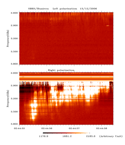
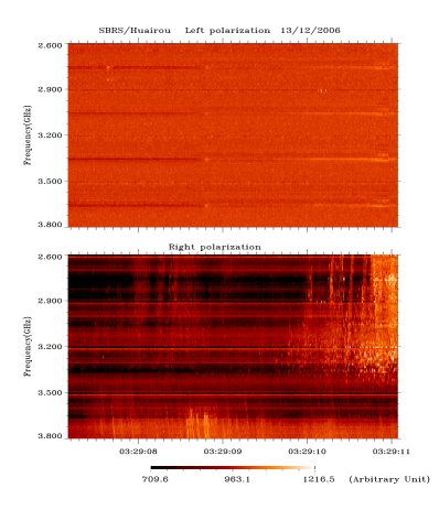
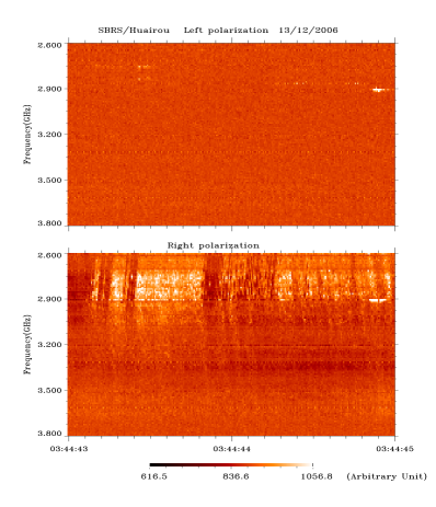
Figure 2: Three groups of microwave type III pairs at 02:44:56 UT (A), 03:29:09 UT (B), and 03:44:43 UT (C) observed at SBRS/Huairou on 2006 December 13. The right-bottom panel shows the the whole flare process profiled by GOES soft X-ray at 1-8 Å  and microwave emission at 3.75 GHz.

Table 1: Estimation of the physical parameters in the source region of type III pairs occurring in the postflare phase of the X3.4 flare on 2006 December 13.

	Parameter	Type III pair A	Type III pair B	Type III pair C
Observation	Start time (UT)	02:45	03:29	03:45
	Lifetime: $\tau$ (s)	0.16	0.10	0.07
	Separate frequency: $f_{x}$ (GHz)	2.92	3.42	2.90
	Frequency Gap: $\delta f$ (MHz)	50	260	10
	Normal III: $f_{stn}$ (GHz)	2.895	3.290	2.895
	$D_{n}$ (GHz s-1)	-14.5$\pm$0.6	-13.1$\pm$0.8	-10.5$\pm$1.2
	$\bar{D}_{n}$ (s-1)	-5.3$\pm$0.22	-4.4$\pm$0.26	-3.8$\pm$0.44
	RS III: $f_{str}$ (GHz)	2.945	3.56	2.905
	$D_{r}$ (GHz s-1)	8.6$\pm$0.8	5.6$\pm$0.6	9.7$\pm$0.8
	$\bar{D}_{r}$ (s-1)	2.6$\pm$0.24	1.5$\pm$0.16	3.2$\pm$0.26
Diagnostics	$n_{x}$ ($10^{17}m^{-3}$)	1.05	1.44	1.03
	$T$ ($10^{7}$ K)	1.85	1.45	1.38
	$n_{n}$ ($10^{17}m^{-3}$)	1.035	1.336	1.035
	$B_{n}$ (G)	87.4$\pm$27.2	80.2$\pm$26.5	70.4$\pm$26.4
	$\beta_{pn}$	0.87	1.05	1.00
	$H_{nn}$ (km)	4.3$\times 10^{3}$	5.3$\times 10^{3}$	5.0$\times 10^{3}$
	$v_{n}$ (c)	0.47	0.45	0.39
	$E_{n}$ (keV)	64.1	58.0	42.3
	$n_{r}$ ($10^{17}m^{-3}$)	1.071	1.565	1.042
	$B_{r}$ (G)	67.6$\pm$21.1	53.6$\pm$17.0	67.8$\pm$25.3
	$\beta_{pr}$	1.50	2.74	1.09
	$H_{nr}$ (km)	7.5$\times 10^{3}$	1.4$\times 10^{4}$	5.5$\times 10^{3}$
	$v_{r}$ (c)	0.47	0.46	0.39
	$E_{r}$ (keV)	64.1	61.0	42.3
	$L_{c}$ (km)	101	733	18

0.86$D$ is frequency drift rate, $\bar{D}$ is the relative frequency drift rate, $f_{0}$ is the central frequency of the type III burst. $f_{x}$ is the separate frequency between the normal type III bursts and the RS type III bursts. $B$ is the magnetic field, $v$ and $E$ are the velocity and energy of electron beams, respectively. $\beta_{p}$ is the plasma beta value. The subscript $n$ and $r$ indicate the normal and RS type III branches, respectively. $L_{c}$: Length of acceleration region.

The flare starts at 02:14 UT, peaks at 02:40 UT. The microwave type III burst pairs occurred at 02:45 UT, 03:29 UT and 03:45 UT, respectively, from several minutes to more one hour after the flare maximum. All type III pairs are strongly right-handed circular polarization overlapping on a long-duration broadband microwave type IV continuum in the postflare phase. According to the Fig.13 of Tan et al. (2010), the distance between the two footpoints of the flaring loop is about $d\sim 2.0\times 10^{7}$ m. Assuming $t_{n}^{-1}\sim 0$ and the flaring loop to be a semicircle, $R_{c}=\frac{1}{2}d\approx 1.0\times 10^{7}$ m. Then, we the diagnostic physical parameters of the acceleration region can be obtained which listed in Table 1. Here, we found the estimated magnetic fields near the acceleration region are from 53.6$\pm$17.0 G to 87.4$\pm$27.2 G. These values are a little less than the result estimated by microwave Zebra pattern structures in the same flare (90 - 200 G, Yan et al. 2007). As we know that the Zebra pattern emission are produced from the interior of the flare loop while the flare primary energy-release sites are above the flare loop. The energy of the electron beam associated to the RS type III branch is in the range of 42 - 64 keV, which is similar to that of the normal type III branches. This fact implies that accelerations are possibly selfsame for the upgoing and downgoing electron beams.

Table 1 also shows that the frequency drift rate of the normal type III branches is higher than that of RS branches. This fact can be explained as following: from Equation (16) we have:

$$\bar{D}\approx\frac{1}{2\mu_{0}k_{B}}\frac{B^{2}}{n_{st}T}\frac{v_{b}}{R_{c}}.$$ (19)

As we know electron beam of the normal type III branches propagates upward in a relatively rarefied plasma ($n_{stn}$) while the electron beam of the RS branches propagates downward in a relatively denser plasma ($n_{str}$): $n_{stn}<n_{str}$. Equation (19) gives: $\bar{D}_{n}>\bar{D}_{r}$, the normal branches drift faster than the RS branches.

Equation (19) shows that not only the plasma density ($n_{e}$) affects the frequency drift rate, but also the magnetic field strength ($B^{2}$), plasma temperature ($T$), magnetic field configuration ($R_{c}$), and the velocity of electron beams ($v_{b}$) dominate the value of drift rates. After determining these parameters, we can really explain the other observed properties of microwave type III burst pairs.

Additionally, we also calculated the plasma beta value ($\beta_{p}$). The result is also listed in Table 1. Here, we find that the plasma beta is much greater than 1 which is just indicating that the flare primary energy-release region is a highly-dynamic area where the magnetized plasma is unstable which may generate plasma instability, trigger magnetic reconnection, accelerate particles, heats the ambient plasmas, release the magnetic energy, and produce the flaring eruptions.

According to PE mechanism, the frequency gap may imply a density difference between start sites of normal and RS type III bursts. With density scale length $H_{n}$, a spatial length can be derived:

$$L_{c}\approx H_{nn}\cdot\frac{\delta f}{2f_{stn}}+H_{nr}\cdot\frac{\delta f}{2f_{str}}.$$ (20)

$L_{c}$ can be regarded as estimation of the length of acceleration regions. The electrons are accelerated in this region and get a relatively high energy, then trigger microwave type III bursts outside this region. The estimated length is about 18 - 733 km. It is possible that these results are the upper length limit of the acceleration region.

In the above estimation, we adopt the same value of $R_{c}$ for both of normal and RS type III branches. Actually, they are different from each other. However, Equation (2) indicates $B\propto R_{c}^{1/2}$, and Equation (4) indicates $v_{b}\propto R_{c}B^{-2}$, these facts show that the beam velocity ($v_{b}$) is independent to the magnetic field strength. So, the uncertainties of magnetic field will not affect the estimation of the velocity and energy of the electron beams.

5 Conclusions and Discussions

In summary, when consider the effect of magnetic field on the plasma density and its distribution around the flare energy-release site, a relationship between the physical conditions and the observing parameters of microwave type III bursts can be established. With this relationship, we can diagnose the flare energy-release sites directly. The diagnostic procedure is as following,

(1) Determine the temperature ($T$) at the time of microwave type III burst from the observation of GOES SXR at wavelength of 0.5 - 4 Å  and 1 - 8 Å.

(2) Determine the plasma density ($n_{x}$) using Equation (6) from the observing start frequency ($f_{st}$) of microwave type III burst or the separate frequency ($f_{x}$) of microwave type III burst pairs.

(3) Estimate the magnetic field ($B_{L}$ and $B_{H}$) by using Equation (17) and (18) from the observing relative frequency drift rate ($\bar{D}$), burst lifetime ($\tau$) and the curvature radius of magnetic field lines ($R_{c}$).

(4) Estimate the velocity and energy of the energetic electron beams using Equation (15) or (16) from the observing relative frequency drift rate ($\bar{D}$), the curvature radius of magnetic field lines ($R_{c}$) and the above derived magnetic field strength ($B$).

(5) As for the microwave type III pairs, we may obtain an upper limit of the length of acceleration region by using Equation (20) from the observed frequency gap ($\delta f$) between the normal and RS type III branches.

In the above diagnostic procedure, there is a key parameter $R_{c}$. In the example of Section 4, we obtained $R_{c}$ by simply using the EUV imaging observation. Generally, such estimation is a bit more exact than to derive the plasma density scale length directly from the existing plasma density models. However, the above method is still a bit cursory. The more exact method to derive $R_{c}$ depends on the radio spectral imaging observations at the corresponding frequencies, such as the Chinese Spectral Radioheliograph (CSRH, now renamed as MUSER, Yan et al. 2009). By using such new generation telescopes, we may directly obtain the location and geometry of the source region, and get the more exact value of the magnetic field scale length.

From the above diagnostics, we may provide basic information for the study of flare triggering mechanism and particle acceleration. However, the above method cannot be extended to meter or longer wavelength type III bursts for their propagating along the open weak magnetic fields in the higher corona. Here, the magnetic field ($B$) becomes very weak and the curvature radius of magnetic field lines ($R_{c}$) becomes very large, $\frac{B^{2}}{n_{x}\mu_{0}R_{c}}\ll m_{0}g$, Equation (13) degenerates to be the barometric format $H_{n}\approx-\frac{k_{B}T}{m_{0}g}$. Then the above diagnostic method will deviate from its correctness.