A Discrete Stochastic Formulation for Reversible Bimolecular Reactions via Diffusion Encounter

Abstract

The classical models for irreversible diffusion-influenced reactions can be derived by introducing absorbing boundary conditions to over-damped continuous Brownian motion (BM) theory. As there is a clear corresponding stochastic process, the mathematical description takes both Kolmogorov forward equation for the evolution of the probability distribution function and the stochastic sample trajectories. This dual description is a fundamental characteristic of stochastic processes and allows simple particle based simulations to accurately match the expected statistical behavior. However, in the traditional theory using the back-reaction boundary condition to model reversible reactions with geminate recombinations, several subtleties arise: It is unclear what the underlying stochastic process is, which causes complications in producing accurate simulations; and it is non-trivial how to perform an appropriate discretization for numerical computations. In this work, we derive a discrete stochastic model that recovers the classical models and their boundary conditions in the continuous limit. In the case of reversible reactions, we recover the back-reaction boundary condition, unifying the back-reaction approach with those of current simulation packages. Furthermore, all the complications encountered in the continuous models become trivial in the discrete model. Our formulation brings to attention the question: With computations in mind, can we develop a discrete reaction kinetics model that is more fundamental than its continuous counterpart?

60J10, 60J50, 60J70, 60J22, 65C35, 65C40, 92C40

1 Introduction

The theory of Brownian motion [15, 48, 63], as developed by Einstein, Smoluchowski, and Langevin, describes the random motion of a particle immersed in a fluid resulting from its collisions with the atoms or molecules of the fluid. There are two distinct physical effects from the collisions: A mean frictional force that resists a macroscopic motion and a random fluctuating force, with zero mean, that rapidly changes the directions of movements. As with any model, the theory itself is a mathematical idealization of the physical reality. For instance, as a continuous function of time, overdamped Brownian motion has a fractal geometry, i.e. between any two instants in time, there is an infinite amount of fluctuations and changes of direction of the particle. However, any physical process that follows Newtonian mechanics always has two times sufficiently close that a particle only moved on a straight line, known as mean free path.

In the current work, we deal with reversible chemical reactions mediated by diffusion in aqueous solution, which is a complex problem built over the Brownian Motion framework. Historically, Smoluchowski, and Collins and Kimball [10, 54] formulated a macroscopic theory for the irreversible formation of a chemical species $C$ from separated $A$ and $B$ compounds in terms of diffusive motions of the reactants, leading to their encounter and chancy transformation. Interestingly, the stochastic process underlying the same diffusion equation and boundary condition, known as partially reflected Brownian motion (PRBM) [19], predetermines an associated process of repeated futile encounter known as a gemination process [2, 3, 8, 11], which plays a central role in both association and dissociation processes. The rigorous mathematical problem of PRBM, however, is non-trivial [7]. It is best understood as the limit of a discrete random walk [9], as explained in detail in the Appendix B.

In practice, most complex problems in applied mathematics are inevitably solved computationally. The continuous mathematical descriptions of Brownian motion problems like the above are eventually discretized into algorithms that are appropriate for numerical computations. One therefore naturally seeks a formulation of applied “Brownian motion” problems directly in terms of a discrete representation. Such an approach, without loss of accuracy and rigor, bypasses two difficult mathematical subjects altogether: continuous stochastic path as the limit of a discrete Markov process and numerical accuracy of high-order discrete algorithm for a continuous problem. The objective of the present work is to follow this approach to develop a discrete stochastic model for reversible bimolecular reactions via diffusion encounter.

It is important to mention that at this point we are not concerned in making a judgment of whether the physical reality is Newtonian or not but on a more computationally accessible approach. Our premise is that all phenomena we observe as the physical reality at some time and space scales, in applied mathematics, can be formulated and implemented as discrete models, which is not necessarily the same as implementing discretization of continuous physical laws. In 1960s computational fluid dynamics (CFD) had a similar problem emerged that was first solved by Godunov in his 1959 revolutionary paper [18]. Before Godunov’s work, the CFD numerical methods for compressible flow were plagued with difficulties. His approach to solve these issues was to provide a discrete conservation law instead of a discretization of a conservation law solely [18, 30, 49, 62]. The model presented herein shares that inspirational spirit; we will formulate a discrete stochastic process instead of a discretization of a continuous stochastic process.

Additional motivation lies in the growing need for quantitative mathematical models, and fast algorithms, of small biological systems like cells or subcellular compartments of the cell. Most of these systems are non-homogeneous in space and have a low number of molecules, so its modeling is based on stochastic reaction-diffusion theory at mesoscopic scales. However, unlike the case of homogeneous reaction theory [6, 46], the connection between the reaction-diffusion phenomena at different microscopic, mesoscopic and macroscopic scales is still a matter of recent research [5, 17, 22, 23, 24]. Our model contribution in this front is to unify the theory of reversible diffusion-influenced reactions [1, 26, 52] with the different approaches to model reversible reactions taken by several simulation packages , like Smoldyn, FPKMC, eGFRD [3, 13, 58] and others [14, 21, 51, 59, 65, 69]. We also note that in a macroscopic phenomenological reaction-diffusion theory the diffusion coefficients of $A$ and $B$ and their association rate constant are three independent parameters [33, 35]. Mechanistically, however, the last is a function of the former two [11, 54]. Our discrete model could also provide a guideline on how to establish these connections for nonlinear reversible reactions.

With the discussion above in mind, we begin with a general approach in the spirit of Langevin [29]. Consider the stochastic dynamic equations for an immersed particle of mass $m$,

$$dx=vdt,\ \ mdv=\big{(}-\eta v+\xi(t)\big{)}dt;$$ (1.1)

where $x$ is the position, $v$ the velocity, $\eta$ the damping coefficient, $\xi(t)$ the white noise term that satisfies $\xi(t)dt=\sqrt{2k_{B}T\eta}\ dW_{t}$ with $W_{t}$ the standard Brownian motion or Wiener process, $k_{B}$ the Boltzmann constant and $T$ the temperature. The Wiener process satisfies $E[W_{t}]=0$ and $E[W_{t}W_{s}]=\mathrm{min}(t,s)$, which implies $E[\xi(t)\xi(s)]=2k_{B}T\eta\delta(t-s)$. The stochastic trajectory in its integral form is given by

$$x(t)=x(0)+\int_{0}^{t}e^{-\eta s/m}\left(v(0)+\frac{1}{m}\int_{0}^{s}e^{\eta\tau/m}\xi(\tau)d\tau\right)ds,$$ (1.2)

and its probability distribution dynamics is described by the multivariate Fokker-Planck equation, which in this specific case, it is usually referred as the Klein-Kramers equation,

$$\frac{\partial\mathit{f}(x,v,t)}{\partial t}=\frac{\partial}{\partial v}\left[\left(\frac{k_{B}T\eta}{m^{2}}\right)\frac{\partial f}{\partial v}+\frac{\eta v}{m}f\right]-v\frac{\partial f}{\partial x}.$$ (1.3)

In the overdamping limit of equation (1.1), we obtain $dx=\frac{1}{\eta}\xi(t)dt,$ which yields a simpler Fokker-Planck equation

$$\frac{\partial f(x,t)}{\partial t}=D\frac{\partial^{2}f(x,t)}{\partial x^{2}},$$ (1.4)

with the diffusion coefficient given by the Einstein relation: $D=k_{B}T/\eta$. This equation describes the probability distribution dynamics of standard Brownian Motion or Wiener process with no drift. Note it can be extended to varying damping coefficient $\eta(x)$, which would make the diffusion coefficient not constant, and it will change the form of the equation. In particular, the issue of Itō vs. Stratonovich or divergence form of the diffusion term matters [4].

Although Eq. 1.4 has an identical form as the classical diffusion equation for a density of particles, it has a much fundamental character; it does not rely on Fick’s law. The classical equation should be understood as the equation of mean density of a large number of identical, independent Brownian particles. Fick’s law then is an emergent statistical phenomenon.

The theory of chemical reaction in aqueous solution, mediated by diffusion encounter, is based on a three-dimensional version of the standard Brownian motion we just presented, with the addition of an absorbing or partially absorbing boundary condition to model the “event of encounter” in a reaction; it is the core of Smoluchowski’s theory [10, 54]. However, as Brownian Motion is such a powerful and useful mathematical idealization, it is easy to assume that it is a first principle. For instance, we tend to think of random walks as approximations to standard Brownian motion (or more accurately to a Wiener Process), immediately assuming Brownian motion is the best description of the physical world. In reality, the theory of Brownian motion is a mathematical limit, and one could even argue Random Walks might provide models closer to what one observes in reality than Brownian motion theory. With computational tasks in mind, why shouldn’t we think standard Brownian motion theory is the one providing an approximation to some specific kind of Random walks?

For relatively simple processes, as in diffusion-influenced irreversible reactions, standard Brownian motion provides a robust theoretical framework. However, when dealing with more complex processes like reversible reactions, a great deal of subtleties arise [1, 3, 8, 26, 40]. Many of the issues one encounters while trying to model more and more complex processes are intrinsic to the fact that one had adopted a specific mathematical idealization, especially when dealing with such an abstract idealization like Brownian Motion. For instance, it has been shown that the continuous diffusion approximation of discrete reaction networks can fail to represent correctly the mesoscopically interesting steady-state behavior of bi-stable systems [66], an issue of utter relevance in biochemical cell dynamics. The purpose of this paper is to convince the reader that an alternate discrete approach to reversible stochastic reaction-diffusion might provide a simpler, more robust, and computation-friendly framework where these subtleties are no longer an issue. It also unifies previous theoretical approaches with more recent simulation algorithms, contributing to a better understanding of reversible stochastic reaction-diffusion. Although the model here presented is for a relatively simple problem, it provides the guidelines for a different line of research that could address fundamental issues in stochastic reaction-diffusion theory and simulations. In the next subsection, we present a condensed review of some of the classical models for bimolecular reactions that are mediated by diffusion encounter.

1.1 Bimolecular reactions mediated by diffusion encounter

Diffusion-influenced reactions. Consider the reaction $A+B\overset{k_{S}}{\longrightarrow}C$, where $A$ and $B$ are two reactive spheres diffusing in space. Fix the frame of reference at the center of $A$ and assume many $B$ particles diffuse around $A$ with a diffusion coefficient given by the sum of $A$ and $B$ diffusion coefficients, $D=D_{A}+D_{B}$, following standard Brownian motion. Whenever the $B$ molecules reach by diffusion the boundary $\sigma$ given by the sum of the radii of $A$ and $B$, $\sigma=R_{A}+R_{B}$, we assume a reaction occurs. We call this reaction a purely diffusion-controlled reaction. Smoluchowski classical work, given in detail in [10, 53, 54], calculates the association rate constant $k_{S}$.

In Smoluchowski’s original work, the concentration of molecule $B$ surrounding the $A$ is denoted by $c(r,t)$. It obeys a simple three-dimensional diffusion equation,

$$\frac{\partial c(r,t)}{\partial t}=\nabla\cdot\big{[}D(r)\nabla c(r,t)\big{]},\ \ r\in[\sigma,R]$$ (1.5a)

$$c(\sigma,t)=0,\ \ c(R,t)=c_{0}.$$ (1.5b)

As the problem is spherically symmetric, we obtain $\frac{\partial c(r,t)}{\partial t}=\frac{D}{r^{2}}\frac{\partial}{\partial r}\left(r^{2}\frac{\partial}{\partial r}c(r,t)\right)$, for constant $D$. The absorbing boundary condition at $\sigma$ represents the purely diffusion-controlled reaction with 100% reaction for each and every encounter; the boundary condition at $R$ provides a bath of $B$ molecules that guarantees a constant concentration, $c_{0}$, at a distance $R\gg\sigma$. The quantity $c_{0}$ is identified as the “bulk concentration” in an aqueous solution containing many $A$’s and $B$’s. In the limit of $R\rightarrow\infty$, the time-dependent and stationary solutions to this equation are given respectively by

$$c(r,t)=c_{0}\left[1-\frac{\sigma}{r}\mathrm{erfc}\left(\frac{r-\sigma}{\sqrt{4Dt}}\right)\right],\ \ \ \ c_{ss}(r)=c_{0}\left[1-\frac{\sigma}{r}\right].$$

The steady state diffusion controlled association rate constant is then obtained from the flux at the reaction radius, $\sigma$, as

$$k_{S}=\frac{4\pi D\sigma^{2}c_{ss}^{\prime}(\sigma)}{c_{0}}=4\pi D\sigma.$$

In the one and two dimensional case, it is worth mentioning that it is not possible to obtain reaction rates in the same manner since the mean first passage times diverge as $R\rightarrow\infty$. There is a large literature on how to deal with this physically very different and mathematically challenging problem [40, 41, 42, 50]. Also, as pointed out in [10], the time-dependent flux becomes infinite at $t=0$, which is unacceptable when the initial rate may be very significant. These issues, among others pointed out in [10], are weaknesses of the theory.

Collins and Kimball gave an improvement over Smoluchowski’s theory [10], in which the absorbing boundary at $\sigma$ is replaced with a partially absorbing boundary condition. This is obtained by making the flux equal to the concentration at the reaction radius,

$$\left.4\pi\sigma^{2}D\frac{\partial c(r,t)}{\partial r}\right|_{r=\sigma}=\kappa c(\sigma,t),$$ (1.6)

where $\kappa$ controls the degree of diffusion-influence in the reaction ($\kappa=0$ means no reaction, while $\kappa\rightarrow\infty$ means the reaction is diffusion limited). In stochastic simulations, $\kappa$ is intimately related to the probability of being absorbed ($p$) or being reflected. But the relation is non-trivial as signified by the dimension of $\kappa$: [length]³[time]^-1. In fact, both $D$ and $\kappa$ are best understood in terms of a discrete setting: $D=\frac{\Delta x^{2}}{6\Delta t}$ and $\frac{\kappa}{4\pi\sigma^{2}}=\frac{\Delta x}{\Delta t}p$, see Appendix B.

Solving Eq. 1.5a with $\frac{\partial c(r,t)}{\partial t}=0$ and with this boundary condition yields the steady state, and the partially absorbing reaction rate of Collins and Kimball,

$$c_{ss}(r) = c_{0}\left[1-\frac{\kappa\sigma}{4\pi D\sigma+\kappa}\left(\frac{1}{r}\right)\right],$$ (1.7)

$$k_{CK} = \frac{\kappa k_{S}}{\kappa+k_{S}}.$$ (1.8)

Note that if $\kappa\rightarrow\infty$ we recover the purely diffusion limited reaction rate $k_{S}$. Furthermore, in the full time dependent solution with the new boundary condition, the flux will no longer be singular at $t=0$ [10].

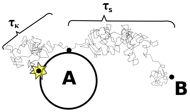
The reaction rates defined through steady-state flux, given in Eq. 1.8, have a clear probabilistic interpretation in terms of the mean passage times, $\tau$ [53, 57]. We can assume $\tau_{CK}=\tau_{S}+\tau_{\kappa}$, where $\tau_{CK}$ is the mean passage time until the first reaction occurs in the Collins and Kimball model, $\tau_{S}$ is Smoluchowski’s mean first passage time from a uniform distribution outside the absorbing boundary to the absorbing boundary, and $\tau_{\kappa}\sim\kappa^{-1}$ is the mean passage time starting from the absorbing boundary until the molecule is bound, this is illustrated in Figure 1. Note Eq. 1.8 is immediately recovered by using the inverse relation $\tau_{CK}\sim 1/k_{CK}$. A reaction is reaction-probability limited if $k_{S}\gg\kappa$, such that $k_{CK}\approx\kappa$. Therefore, Collins and Kimball’s theory is applicable to cases ranging from diffusion-limited scenario $k_{S}\ll\kappa$ to reaction-probability-limited scenario.

Figure 1: Interpretation of the times corresponding to the inverse of the reaction rates in the Collins and Kimball model. Note that after a time $\tau_{S}$ when particle $B$ collides with $A$, the reaction might not happen; it still has to wait a time $\tau_{\kappa}$. This is the stochastic trajectory interpretation of a partially absorbing boundary. In a more formal interpretation PRBM should be understood as purely reflective Brownian Motion conditioned to stop at a random time [9, 19], see Appendix B.

The reaction diffusion problems framed as above can equivalently be described in terms of the Green’s functions for an isolated pair of $A$ and $B$ molecules [64, 65]. Consider again one molecule $A$ fixed in the origin. We will denote $f(r,t|r_{0})$ the probability of a particle $B$ being a distance $r$ from $A$ at time $t$ given that it was at $r_{0}$ at time $0$. This transition probability will obey the diffusion equation, initial condition and boundary condition,

$$\frac{\partial f(r,t|r_{0})}{\partial t}=\nabla\cdot\big{[}D(r)\nabla f(r,t|r_{0})\big{]}.$$ (1.9a)

$$f(r,0|r_{0})=\frac{\delta(r-r_{0})}{4\pi r_{0}^{2}}.$$ (1.9b)

$$\lim_{r\rightarrow\infty}f(r,t|r_{0})=0,$$ (1.9c)

and an extra boundary condition at $r=\sigma$, which can be Eq. (1.5b) or Eq. (1.6) written in terms of $f(r,t|r_{0})$. Note this is an equation for the probability $f(r,t|r_{0})$, which is the “remaining” probability density function in the presence of an absorbing or partially absorbing boundary (diffusion with killing). Then

$$-\frac{d}{dt}\int_{\sigma}^{\infty}4\pi r^{2}f(r,t|r_{0})dr$$

is the probability density function for the absorbing time.

Reversible bimolecular reaction via diffusion encounter. The Green’s function formulation for an isolated pair has been extended to modeling reversible reactions in one, two and three dimensions [1, 26, 40]. For spherical symmetry and constant $D(r)=D$, these extensions consist of augmenting boundary condition (1.6) with a “back-reaction” with rate $\mu$:

$$\left.4\pi\sigma^{2}D\frac{\partial f(r,t|r_{0})}{\partial r}\right|_{r=\sigma}=\kappa f(\sigma,t|r_{0})-\mu\big{[}1-S(t|r_{0})\big{]},$$ (1.10)

$$\mathrm{where}\hskip 5.69054ptS(t|r_{0})=1-\int_{0}^{t}4\pi\sigma^{2}D\left.\frac{\partial f(r,\tau|r_{0})}{\partial r}\right|_{r=\sigma}d\tau,$$

and $S(t|r_{0})$ is referred as the survival probability in the literature. An analogous version of the boundary condition in (1.10) first appeared in [52], which also made an important statement that in a chemical reaction equilibrium, the $\lim_{t\rightarrow\infty}f(r,t|r_{0})$ should be uniform in space independent of $r$.

The notion of survival probability doesn’t really make sense when talking about reversible reactions. A more appropriate name for $S(t|r_{0})$ is the probability of $B$ not being bound at time $t$ given it initially was a distance $r_{0}$ from $A$, regardless if the particle was bounded at some time between $0$ and $t$. This is clear from the fact that

$$S(t|r_{0})= 1-\int_{0}^{t}4\pi\sigma^{2}D\left.\frac{\partial f(r,\tau|r_{0})}{\partial r}\right|_{r=\sigma}d\tau$$ (1.11)

$$= \int_{\sigma}^{\infty}4\pi r^{2}f(r,t|r_{0})dr,$$

which is easily proved by differentiating Eq. 1.11 by $t$, then using Eq. 1.9a and the boundary conditions, then repeat the inverse process and evaluate at $t=0$ to find the integration constant to be one. The second integral is clearly the probability of being unbound as we mentioned before. The exact solution of this problem is given in [26]. In [39, 38], the authors implemented numerical simulations using this model as a starting point.

If one restricts the diffusion of $B$ in a finite space and replaces Eq. 1.9c with a reflecting boundary at $R$, then the stationary equilibrium solution to Eq. 1.9a with boundary condition Eq. 1.10 gives $f_{eq}(r)\equiv f_{eq}(\sigma)=(\mu/\kappa)p_{C}$ in which $p_{C}$ is the equilibrium probability of $C$: $p_{C}=1-f_{eq}(\sigma)V_{B}$, where $V_{B}=\frac{4\pi}{3}\big{(}R^{3}-\sigma^{3}\big{)}$ is the volume available to the diffusing $B$ [52]. Therefore, the theory provides a rigorous equilibrium constant for the reversible association reaction

$$K_{eq}\equiv\left(\frac{p_{C}}{1-p_{C}}\right)V_{B}=\frac{\kappa}{\mu}.$$ (1.12)

This implies that if the bimolecular association rate constant is $\kappa$, then the unimolecular dissociation rate constant has to be $\mu$. On the other hand, if we choose Eq. 1.8 as the on-rate constant $k_{\mathrm{on}}=\kappa k_{S}/(k_{S}+\kappa)$, as suggested by Fig. 1, then the off-rate constant has to be $k_{\mathrm{off}}=\mu k_{S}/(k_{S}+\kappa)$. The validity of Eq. 1.12 assumes two well-defined states, $A+B$ and $AB\equiv C$, with Markov transition in between. Strictly speaking, this requires the dynamics within each of the two states to be sufficiently rapid while the transitions between the two states as relatively rare events. “Diffusion finally manages to separate the reaction partners.” [8]. Additionally, these rates can be interpreted as

$$k_{\mathrm{on}}=k_{S}\frac{\kappa}{k_{S}+\kappa}=k_{S}\phi,$$ (1.13)

where $\phi=\kappa/(k_{S}+\kappa)$ can be understood as the fraction of geminate recombinations that lead to association or also as the probability of association at the boundary. Then the off rate is

$$k_{\mathrm{off}}=\mu\frac{k_{S}}{k_{S}+\kappa}=\mu(1-\phi),$$ (1.14)

where the probability of dissociation at the boundary is $\big{(}1-\phi\big{)}$. The reverse reaction rate constant $k_{\mathrm{off}}$ has the property that it is diffusion controlled if, and only if, $k_{\mathrm{on}}$ is diffusion controlled, quite irrespective of the value of $\mu$. “[A]ny description of the reaction process that divides the initial bimolecular event into a diffusive association step [$\cdots$] and a subsequent unimolecular transformation is logically incorrect.” [52]. This means that in the case of reversible bimolecular reactions, we should not treat association and dissociation as independent processes .

For simplicity, all the models presented in this section assumed there is no force field. However, all the models have generalizations that introduce a force field through a potential; they can all be found in the literature cited.

2 Reaction-diffusion as a discrete stochastic process

In this section, we will present the theoretical basis and motivation to model reaction-diffusion as a discrete stochastic process. As mentioned in the previous section, all the subtle issues that cause confusion among the existing theories of reversible reactions with diffusion become trivial when moving to an appropriate discrete time/space stochastic description. This will shed some light in the advantages of the discrete stochastic models presented in the next section. It should be noted that similar successful attempts have been made to write one and two dimensional irreversible Smoluchowski type models as discrete stochastic processes [60, 61, 68]. We will break down our attention into three different aspects:

1. Reactions as stochastic processes and their two descriptions, e.g., ensemble distribution and sample trajectories.

2. Definition of bound/unbound in $A+B\xrightleftharpoons[]{}C$.

3. Simulations with geminate recombinations. Gemination is the process described by $\tau_{\kappa}$ in Fig. 1.

Although these three aspects are closely related to each other, the sequential presentation illustrates some of the advantages of our discrete stochastic model from slightly different angles. Some of the subtle issues that come up in the classical models will be discussed in the different sections, and it will be addressed how the discrete stochastic description helps solving them. Each of these aspects will be covered in detail in the following subsections.

2.1 Reactions as stochastic processes and their two descriptions

Well stirred chemical reactions where there is no spatial component in the equations have been successfully modeled with deterministic models based on the Law of Mass Action (LMA). However, for cellular biochemical processes inside individual cells, the number of molecules might not be large enough for an accurate continuous description. In this case, there is a unifying stochastic mathematical framework known as the Delbrück-Gillespie process, whose Kolmogorov forward equation (KFE) has been known as the Chemical Master Equation (CME), and whose stochastic trajectories can be computed with the Gillespie, or Doob-Bortz-Kalos-Lebowitz, algorithm [45, 46]. Although spatial homogeneity is still assumed in this theory, its depth and richness lie in Kurtz’s theorem, stochastic nonlinear bistability [47], and stochastic oscillations. This theory has provided a better understanding of biochemical bistability, as shown by a deterministic and stochastic comparison of the Schlögl model [66], and in the separation between the dynamics at short and long time scales.

The Delbrück-Gillespie process is a landmark example, at least in chemical reaction dynamics, of the two parallel descriptions of a stochastic process. Its CME describes the time-evolution of the probability distribution while the Gillespie algorithm describes the stochastic trajectory of the system, one reaction at a time, whose statistical ensemble properties will satisfy such probability distribution. The same dual description is of key importance when it comes to producing particle-based numerical simulations. One may know (or think to know) the KFE of a diffusion process; however, if we cannot obtain the stochastic trajectories from it, it becomes very difficult to produce accurate particle-based numerical simulations. In theoretical mathematics, this is the task of constructing a Markov process from its infinitesimal generator [36]. This is precisely the case of the continuous reversible diffusion-influenced reactions modeled with the back-reaction boundary condition from Eq. 1.10. The boundary condition obscures the underlying stochastic process and consequently complicates any particle-based simulation. This is the reason why we need a more transparent formulation as the one presented in this paper, where the nature of the stochastic process is simple from the beginning. On the theoretical side, we have also noted that while Kurtz’s theorem provides a rigorous and satisfying mathematical foundation, in probabilistic terms, for the LMA, the theory of hydrodynamic limit as the foundation of nonlinear partial differential equations of reaction-diffusion type is far from complete and still only accessible to experts [5, 17].

2.2 Definition of bound/unbound state in $A+B\xrightleftharpoons[]{\quad}C$

Chemical reactions are considered as discrete events. But at an atomic scale, the very definition of a $B$ that is bound ($C$ state) or unbound to an $A$ molecule is not unequivocal. This is particularly the case for diffusion-influenced reaction [43], which can yield significantly different quantitative descriptions due to different laboratory measurements. We give two such possibilities, both have been used in experiments that define $C$:

• Distance: FRET (Förster resonance energy transfer) method directly measures the distance between two optical markers that are attached on $A$ and $B$ respectively. Therefore, for this type of data, we say molecule $B$ is bound to $A$ if the distance between the two molecules is less or equal to $\sigma$. We call $r=\sigma$ the absorption or reaction boundary.

• State: Spectroscopic methods differentiate atomic structures of a particular chemical group inside a molecule. If an optically active chemical group (OACG) in $B$ normally adopts a structure $b$ but a very different structure $b^{*}$ near $A$, then the spectroscopic signals become a definition for $B$ versus $C$. Therefore, we say molecule $B$ is bound to $A$ if the OACG inside $B$ is in the $b^{*}$ state; the molecule is unbound if the OACG is in the $b$ state. However, all atomic structures in a molecule fluctuate. In a stochastic setting, the group in $B$ still has a finite probability of adopting the $b^{*}$ structure, while also having a non-zero probability of being in state $b$ when very near $A$. Note in biochemistry, the biological function of a molecule is usually associated with the state of a chemical group within.

In a well-defined bimolecular reaction, the small probabilities of a $B$ with its OACG in the $b^{*}$ state, and a $B$ bound to $A$ with its OACG in the $b$ state, are negligibly small. Therefore, the two definitions above are usually equivalent.

As a simple example, consider a molecule $B$ diffusing in three dimensions with particle $A$ fixed at the origin $r=0$. Assume the intra-molecular potential is described by a Lennard-Jones potential. In this case, it is possible to choose the location of the absorption boundary in the separatrix of the effective potential, so the state and distance definition match each other, as shown in Fig. 2a. However, there are many other possibilities. For instance, in Fig. 2b, we chose the absorption boundary arbitrarily, so it is necessary to decide if $B$ is bound to $A$ when it crosses the absorption boundary (distance) or when it is close to the local minima of $U_{eff}(r)$ (state). In the latter case, it is not even clear the absorbing boundary can model the reaction accurately, so we have to ask the question: does it even make sense to have an absorbing boundary?

Figure 2: Plots of the effective interaction potential $U_{eff}(r)=V\left[\left(\frac{r_{m}}{r}\right)^{12}-2\left(\frac{r_{m}}{r}\right)^{6}\right]-\ln{4\pi r^{2}}$ that molecule $B$ undergoes, where $r$ is the inter-particle distance, $V$ is the depth of the local minima and $r_{m}$ the local minima position. The effective potential takes into account a Lennard-Jones potential and the three dimensional geometrical drift terms. The corresponding $b^{*}$ and $b$ states of the OACG are marked in the potential. The left plot (a) shows when the absorbing boundary location matches the expected behavior under the interaction potential. The plot on the right (b) shows an example that the absorbing boundary location can be chosen arbitrarily. In the latter case, it is not clear that the absorbing boundary models the reaction correctly.

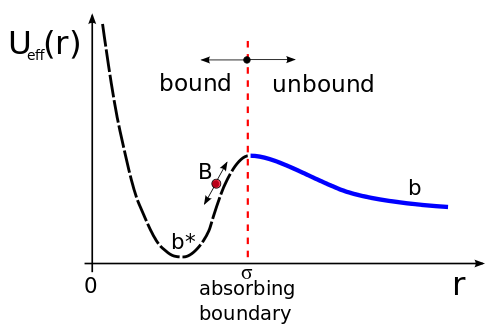
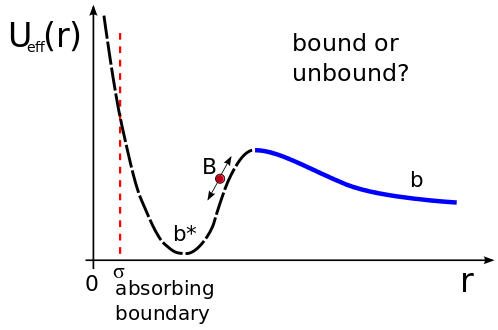
The answer is: it depends on the physics one is trying to model. For instance, in the context of diffusion under an interaction potential, all irreversible reaction models need an absorbing boundary. Without it, there is always a nonzero probability of the full reverse reaction to occur. In this case, the choice of the boundary location cannot be completely arbitrary; it needs to be chosen based on experimental data or obtained via more fundamental interactions, such as the Lennard-Jones interaction. One approach that could provide a solution would relate Kramers’ theory [20, 27] applied to the diffusion under a Lennard-Jones potential with Smoluchowski’s type models. A similar attempt has been studied before for a double well potential elsewhere [53].

In the case of reversible reactions, a similar reasoning can be applied, though the concept of absorbing boundary needs to be replaced by a reaction boundary. However, it is also possible to model reversible reactions without employing a reaction boundary at all. They can be modeled as a diffusion process under a bistable effective interaction potential, like the one shown in Figs. 2, where one state corresponds to $B$ being bound and the other to $B$ being unbound. As a matter of fact, any model that employs a reaction boundary should be fitted to this more general view of a reversible reaction. Although there has been some work in this direction [53], it is still not yet fully understood how to establish the connection between Kramers’ theory applied to reversible unimolecular reaction [20, 27] and the theory of reversible bimolecular reaction mediated by diffusion.

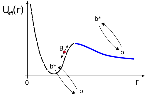
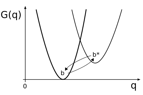
A more complicated example is given in Fig. 3a, where the state of the OACG can oscillate stochastically independent of the distance $r$. In this case, the effective potential is much more complicated than just a Lennard-Jones potential. As a matter of fact, it is a potential landscape that can depend on more variables than just $r$. In this scenario, the state definition can be extended, at least conceptually, to very complicated potential landscapes that could even be stochastic and dynamic. For instance, in Fig. 3b, the two OACG states are given in terms of two Gibbs free energy potentials $(G)$ as a function of the reaction coordinate $q$, like in Marcus theory of electron transfer [34]. In these cases, the state description could become completely detached from the distance description.

Following this analysis, we can say that describing a reversible bimolecular reaction solely through diffusion within its multivariate potential landscape is a more general approach, which corresponds to the state definition. Conversely, the models with a reaction boundary are an approximation to this more general description, which would correspond to the distance definition. This two definitions can be matched if the potential only depends on the inter-particle distance $r$, and we choose a distance close to the separatrix of the potential. It should be noted there is always the possibility that the potential corresponds to an external forcing, or that the absorbing/reacting boundary is actually modeling an absorbing membrane.

These results bring attention to the fact that reaction boundaries are in some sense “artificial”. From a continuous mathematical point of view, a Brownian particle could cross a spatial boundary an infinite amount of times in a finite time, which provides a very non-intuitive description of what is physically happening at the reaction boundary and how to implement a discrete particle-based simulation. This is also intimately related to the issue of geminate recombinations, and it is partly the reason why particle-based modeling of reaction boundaries is non-trivial. In order to do so, one needs to discretize continuous Brownian Motion into a random walk, then somehow provide a discrete model of the reaction boundary, such that in the continuous limit the ensemble average over many identical systems satisfies the continuous equation and the reaction boundary condition. One can come up with multiple ideas on how to do this, but providing one with mathematical rigor is not trivial [9], especially when the reaction boundaries are complex like in Eq. 1.10.

2.3 Geminate recombinations

Geminate recombinations occur when a particle $B$ that just dissociated from a certain $A$, immediately associates again with it. They have been a subject of extensive research [2, 3, 25, 39, 40], and they are fundamental in providing accurate stochastic reaction-diffusion models and algorithms at cellular and sub-cellular level. They are also intimately related to the definition of bound and unbound we discussed in the previous subsection.

In order to gain a better physical insight, we can observe them in the context of irreversible reactions with partially absorbing boundaries and Kramers’ theory [20, 27]. Consider three-dimensional diffusion of a $B$ molecule under a double well potential $U_{eff}^{*}(r)$, like shown in Fig. 3c. Two models will be considered. The first one uses a fully absorbing boundary at the first well $r=\sigma_{1}$ and the second one a partially absorbing boundary at the second well $r=\sigma_{2}$. It has been shown that in the steady state the $\kappa$ parameter of the partially absorbing boundary can be calculated using Kramers’ theory, allowing the two models reaction rate to match each other [53]. This result shows that the partially absorbing boundary at $r=\sigma_{2}$ is equivalent to a fully absorbing one at $r=\sigma_{1}$ . As we know from [8, 9, 19, 52], partially absorbing boundary conditions can be understood as a model for geminate recombinations. The picture just presented favors this view, since the partially absorbing boundary at $\sigma_{2}$ can effectively model the back and forth diffusion in the interval ($\sigma_{1}$,$\sigma_{2}$) before the reaction is finally completed. This back and forth diffusion is also represented by the rebinding diffusion process previously observed in Fig. 1, and it is what we understand as geminate recombinations.

Figure 3: The left plot (a) is the same than Fig. 2 with the addition of stochastic oscillations of the OACG that are independent of $r$. The center plot (b) shows the Gibbs free energy potential for the two possible states of the $B$ molecule as a function of the reaction coordinate. The right plot (c), shows how geminate recombinations can be interpreted in the context of diffusion under the interaction potential $U_{eff}^{*}(r)$, where $r$ is the inter-particle distance. This effective potential takes into account a double well potential and the three dimensional geometrical drift terms.

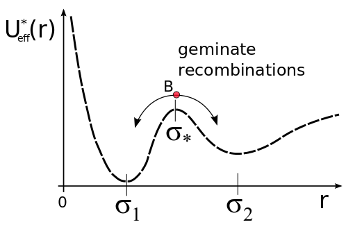
The previous result states that our partially absorbing models of irreversible reactions do take into account geminate recombinations. However, there is still an absorbing boundary, so the dissociation process is not fully modeled. In order to do so, we need to introduce the back-reaction boundary condition at the reaction boundary, which is given by a partially absorbing boundary condition with the addition of the back-reaction term, as in Eq. 1.10. This model was first solved exactly in one dimension and later on in two and three dimensions [1, 26, 40]. However, the solution is not simple, and it’s hard to grasp some physical intuition out of it. It is also based on a non-local boundary condition, and it is not clear, from a rigorous mathematical point of view, what is the corresponding stochastic process behind the partial differential equation (PDE) for the probability. This last issue is relevant because it doesn’t allow us to accurately derive a particle-based stochastic simulation of the trajectories that in average will satisfy the probability described by the PDE. Algorithms like eGFRD [58] and FPKMC [13] are used to simulate reversible reactions using exact solutions for reactions between an isolated pair. However, they do not use solutions for the back-reaction boundary; they use the solution for the partially absorbing boundary and model the dissociation process with an exponential waiting time. It is not obvious nor trivial to show that these two approaches are equivalent.

The model presented in the next section bypasses these issues by framing the problem as a discrete Markov chain. Its Markovian nature allows simple and accurate particle-based simulations that obey the expected statistical behavior given by the KFE. The events occurring at the reaction boundary, including geminate recombinations, are intuitive and easily obtained from the jump probabilities. It also provides a robust and consistent stochastic description that can model reactions using a distance or state approach. In the continuous limit, it recovers the classical models along with the different boundary conditions. It also works as a unifying model since it shows other approaches to model reversible reactions like eGFRD and FPKMC are consistent with the stochastic trajectories of the PDE with the back-reaction boundary condition. It provides further validation for the continuous back-reaction model for diffusion-influenced reactions since the more intuitive discrete reversible reaction particle-based algorithm converges to it. The discrete model’s robustness and particle-based simulations simplicity lie in its rigorous formulation as a discrete stochastic process and its consequent intrinsic relation between the probability distribution dynamics and its individual stochastic trajectories.

3 The discrete stochastic model for diffusion-influenced reactions

The main idea is to create an intuitive Markov jump process, that can be interpreted as a discretization of Eq. 1.9a that conserves probability. The reaction process at the reaction boundaries is intuitively modeled adding association and/or dissociation jump probabilities. On the continuous limit, the continuous equation and the different boundary conditions are recovered, specifically providing additional validation for Eq. 3.32. As it is a discrete time and space stochastic model (Markov chain), it is easy to implement a numerical simulation for the probability mass function as well as a particle based simulation for the individual stochastic trajectories of the reaction process. We will begin by deriving the framework of the model with a radial random walk, and we will add complexity as we recover the different classical diffusion-influenced reaction models. It should be noted that in all the next models we can take the limit $dt\rightarrow 0$ to obtain a master equation and use a variant of the Gillespie Algorithm to solve it numerically. However, we believe the discrete time approach is educational since it provides a clear connection between the parameters in diffusion-influenced theory and their probabilistic meaning in particle-based simulations, see Eqs. B.2 in Appendix B.

3.1 Radial random walk with spherical symmetry

We would like to construct a random walk with spherical symmetry that recovers the Brownian motion diffusion equation in the continuous limit. We will start by considering a particle following a random walk in spherical coordinates. We will only be interested in the jumps between different spherical shells in the $r$ direction separated a distance $\delta_{r}$ and not along the angular directions. If the particle is in shell $i$ with radius $r_{i}=\sigma+i\delta r$ and $\sigma$ a constant, the probabilities to jump to the smaller and bigger shells are $p_{i}$ and $q_{i}$ respectively. The process is partially illustrated in Fig. 4.

We can write this process as a discrete time Markov chain. Let the position in the radial direction be denoted by $\mathcal{R}_{t}$, a random variable for every given $t$ constituting a discrete state and time stochastic process. We will call $\pi^{t}_{i}=\Pr[\mathcal{R}_{t}=r_{i}]$ the probability of being at spherical shell $i$ at time $t$. The state of the whole system at time $t$ is given by the vector of all states $\boldsymbol{\pi}^{t}=\left[\pi^{t}_{0},\pi^{t}_{1},\cdots,\pi^{t}_{i},\cdots\right]$. The dynamics of our random walk are given in terms of the stochastic matrix $\mathbb{P}$ and the Kolmogorov forward equation,

$$\boldsymbol{\pi}^{t+1}=\boldsymbol{\pi}^{t}\mathbb{P}.$$ (3.15)

Note the stochastic matrix should depend on the probabilities $p_{i}$ and $q_{i}$. The resulting stochastic matrix is

$$\mathbb{P}=\left[\begin{matrix}1-q_{0}&q_{0}&0&\cdots&&\cdots\\ p_{1}&1-(p_{1}+q_{1})&q_{1}&0&&\\ \vdots&&\ddots&&&\\ &0&p_{i}&1-(p_{i}+q_{i})&q_{i}&\cdots\\ \vdots&&&\vdots&\ddots&\end{matrix}\right]$$ (3.16)

Note the rows sum to one as expected. For practical purposes, the matrix can be truncated using a finite number of shells $N$. In all theses models, we will assume no-flux boundary conditions in the outermost shell, unless stated otherwise. In order to recover Brownian diffusion, we need to adjust the jump probabilities in the random walk in spherical coordinates with

$$\begin{split}p_{i}=\delta t\left(\frac{D}{\delta r^{2}}-\frac{D}{r_{i-1}\delta r}\right),\ \ \ \ q_{i}=\delta t\left(\frac{D}{\delta r^{2}}+\frac{D}{r_{i+1}\delta r}\right),\end{split}$$ (3.17)

where $D$ is the constant diffusion coefficient. Note the probability of staying in the shell $i$ given by $1-(p_{i}+q_{i})$ grows approaching $1-2\delta tD/\delta r^{2}$ as $r_{i}$ is increased. Using these values we can rewrite the $i^{\mathrm{th}}$ equation of (3.15) as,

$$\pi_{i}^{t+1}=\pi_{i}^{t}+\delta tD\left[\frac{\pi_{i-1}^{t}-2\pi_{i}^{t}+\pi_{i+1}^{t}}{\delta r^{2}}\right]-\delta t\frac{2D}{r_{i}}\left[\frac{\pi_{i+1}^{t}-\pi_{i-1}^{t}}{2\delta r}\right]+\delta t\frac{D}{\delta r}\left[\frac{\pi_{i}^{t}}{r_{i}-\delta r}-\frac{\pi_{i}^{t}}{r_{i}+\delta r}\right].$$

We would like to recover a continuous equation for the probability. The discrete probability $\pi_{i}^{t}$ is related to the continuous probability distribution function $\Pi(r_{i},t)$ by $\pi_{i}^{t}=\Pi(r_{i},t)\delta r$, so we need to divide $\pi_{k}^{t}$ by $\delta r$ for all $k$ first. However this doesn’t make any difference in structure of the equation, so now we can take the limit as $\delta_{t}\rightarrow 0$ and $\delta_{r}\rightarrow 0$ following standard finite difference theory [31], which yields second order accuracy in space and first order in time. We obtain,

$$\frac{\partial\Pi(r,t)}{\partial t}=D\frac{\partial^{2}\Pi(r,t)}{\partial r^{2}}-\frac{2D}{r}\frac{\partial\Pi(r,t)}{\partial r}+\frac{2D}{r^{2}}\Pi(r,t),$$ (3.18)

where $\Pi(r,t)$ is a probability distirbution function in $r$. This equation can be written in the form of a Fokker Planck equation with drift,

$$\frac{\partial\Pi(r,t)}{\partial t}=D\frac{\partial^{2}\Pi(r,t)}{\partial r^{2}}-\frac{\partial}{\partial r}\left(\frac{2D}{r}\Pi(r,t)\right).$$ (3.19)

The probability of being a distance $r$ from the origin at time $t$ is $\Pr\{r<\tilde{\mathcal{R}}_{t}\leq r+\delta r\}=\Pi(r,t)dr$, where $\tilde{\mathcal{R}}_{t}$ is now a stochastic process with continuous state and time. However, this is the probability of being at any point in the sphere with radius $r$, so we cannot yet compare it with the Smoluchowski diffusion equation. In order to do so, we need the equation for the probability of being at any point in space given by $f(r,\theta,\phi,t)r^{2}\sin(\theta)drd\theta d\phi$. Integrating this equation in the angular coordinates yield the probability $\Pi(r,t)$. As we have spherical symmetry in $f$, this yields

$$\Pi(r,t)dr=4\pi r^{2}f(r,t)dr.$$ (3.20)

Substituting this result into Eq. 3.19 and doing some algebra, we recover the Smoluchowski equation (Eq. 1.5a) for constant $D$ as expected,

$$\frac{\partial f(r,t)}{\partial t}=\frac{D}{r^{2}}\frac{\partial}{\partial r}\left(r^{2}\frac{\partial f(r,t)}{\partial r}\right)=\nabla\cdot[D\nabla f(r,t)],$$ (3.21)

where $\nabla$ operates in spherical coordinates with symmetry in the polar and azimuthal angle; therefore, the discrete time Markov chain models the discrete analog to overdamped Brownian motion in spherical coordinates. However, we haven’t yet discussed the continuous limit in the discrete boundary of the innermost shell $r_{0}$. We can also write the first equation of (3.15) as,

$$\pi_{0} {}^{t+1}=\pi_{0}^{t}+\delta tD\left[\frac{\pi_{1}^{t}-\pi_{0}^{t}}{\delta r^{2}}\right]-\delta t\left[\frac{D}{r_{0}}\frac{\pi_{1}^{t}}{\delta r}+\frac{D}{\delta r}\left(\frac{\pi_{0}^{t}}{r_{0}+\delta r}\right)\right].$$

In order to find what boundary condition this discretization satisfies, we will follow standard finite difference techniques [31]. We will introduce the ghost cell $\pi_{-1}^{t}$, so we can rewrite this equation as,

$$\pi_{0} {}^{t+1}=\pi_{0}^{t}+\delta tD\left[\frac{\pi_{1}^{t}-2\pi_{0}^{t}+\pi_{-1}^{t}}{\delta r^{2}}\right]-\delta t\frac{2D}{r_{0}}\left[\frac{\pi_{1}^{t}-\pi_{-1}^{t}}{2\delta r}\right]+\delta t\frac{D}{\delta r}\left[\frac{\pi_{0}^{t}}{r_{0}-\delta r}-\frac{\pi_{0}^{t}}{r_{0}+\delta r}\right],$$

where

$$\pi_{-1}^{t}=\pi_{0}^{t}\frac{\left(\frac{1}{\delta r}-\frac{1}{r_{-1}}\right)}{\left(\frac{1}{r_{0}}+\frac{1}{\delta r}\right)}.$$ (3.22)

Dividing by $\delta r$ and taking the limit $\delta_{t}\rightarrow 0$, $\delta_{r}\rightarrow 0$, we again recover Eq. 3.18 with second order accuracy in space and Eq. 3.22 becomes the zero flux condition for the Fokker-Planck equation (see Appendix A),

$$\left.\frac{\partial\Pi(r,t)}{\partial r}\right|_{r=r_{0}}=\frac{2\Pi(r_{0},t)}{r_{0}}.$$

Using this result and employing Eq. 3.20, the reflective boundary condition for Eq. 3.21 can be rewritten as $\left.\frac{\partial f(r,t)}{\partial r}\right|_{r=r_{0}}=0$, as expected. Note we assumed $r_{0}-\delta r>0$. Unless stated otherwise, in this and all of the subsequent models we will also employ a zero flux boundary on the outermost spherical shell $r=r_{max}$. As we have an irreducible and aperiodic Markov chain with a finite number of states, we know it has a steady state. Moreover, as the flux is zero on both boundaries, the detailed balance condition must be satisfied everywhere. Detailed balance will be mentioned in more detail on Section 3.4. In order to recover the Smoluchowski diffusion equation (Eq. 1.5a) in the whole space, we can take the limit as $r_{0}\rightarrow 0$ and $r_{max}\rightarrow\infty$.

It should be noted that the limit $\delta_{t}\rightarrow 0$, $\delta_{r}\rightarrow 0$ will only guarantee our discretization is consistent with the continuous model. In order for the method to be convergent in the finite difference sense, we also need to satisfy a CFL condition that we can obtain through stability analysis [31]. However, this discretization is also a Markov chain, so we can also obtain a stability condition by making sure that all the rows of matrix 3.16 sum to one and that all the entries are in the interval $[0,1]$. This analysis yields the condition that $\frac{\Delta t}{\Delta r^{2}}<\frac{1}{2D}$, which happens to be the same as the CFL condition for the one-dimensional diffusion equation. When we add more complexity in the next sections, like boundary reaction terms and potentials, we need to be careful that our matrix still satisfies these Markov conditions.

On the discrete model, we can also write the diffusion coefficient in terms of the jump probabilities by summing up Eqs. 3.17 to yield Einstein’s relation,

$$D=\frac{\delta r^{2}}{2\delta t}(p_{i+1}+q_{i-1}).$$ (3.23)

This is a more general expression than the obtained in random walks on Cartesian coordinates. On a Cartesian random walk, if the probability of staying in the same spot is zero, we obtain $p_{i+1}+q_{i-1}=1,1/2,1/3$, in one, two and three dimensions respectively, recovering the well known expression $D=\delta r^{2}/(2n\delta t)$ with $n$ the number of dimensions.

In the next section, we will use this spherical random walk to construct a discrete model for irreversible diffusion-influenced reactions.

3.2 Discrete model for irreversible diffusion-influenced reactions

The random walk derived in the previous model does not yet include any reaction. In order to study the reaction $A+B\rightarrow C$, consider again a particle $B$ diffusing under the spherical symmetric random walk in the previous section. In addition, there will be a particle $A$ fixed at the origin. If we define the shell $r_{0}=\sigma$ as the reaction boundary or the binding radius, then we can incorporate the probability of a reaction $P_{b}=\tilde{\kappa}(r)\delta t$. An illustrated description of the process is shown in Fig. (4), and a detailed one-dimensional symmetric version of this model is presented in Appendix B. The stochastic matrix will now look like

$$\mathbb{P}=\left[\begin{matrix}1-(q_{0}+P_{b})&q_{0}&0&\cdots&\\ p_{1}&1-(p_{1}+q_{1})&q_{1}&0&\\ \vdots&&\ddots&&\\ &0&p_{i}&1-(p_{i}+q_{i})&q_{i}\\ \vdots&&&\vdots&\ddots\end{matrix}\right].$$ (3.24)

Note the first row doesn’t sum up to one, since there is a probability of being absorbed, $P_{b}$. In order to recover the total probability, we need to sum this probability to the first row of the stochastic matrix. Furthermore, the association rate $\tilde{\kappa}(r)$ will scale depending on where we chose our reaction boundary to be. A physically reasonable assumption is that the rate $\tilde{\kappa}(r)$ scales inversely to the infinitesimal volume of the reaction spherical shell, $\tilde{\kappa}(r)=\kappa/(4\pi r^{2}\delta_{r})$, where $\kappa$ is the constant rate in the boundary condition of Eq. 1.10 and has units of volume over time. The bigger the shell, the smaller we need $\tilde{\kappa}(r)$ to be in order to keep the model consistent. Furthermore, note the probability of being absorbed at shell $r_{0}=\sigma$ is $P_{b}=\tilde{\kappa}(r_{0})\delta t$, so we can solve for $\kappa$ to obtain $\kappa=4\pi\sigma^{2}P_{b}\delta r/\delta t$. This equation, along with Eq. 3.23, provide the diffusion-influenced theory parameters $D$ and $\kappa$ in terms of the jump probabilities. As shown in the Appendix B, the probability of being absorbed could be replaced by a more accurate value $P_{b}=1-e^{-\tilde{\kappa}(r_{0})\delta t}$, in which case $\kappa=-4\pi\sigma^{2}\delta r\log{[1-P_{b}]}/\delta t$. However, this is not relevant in the continuous limit analysis we will now carry out.

Figure 4: Concentric shells for the discrete model for irreversible diffusion-influenced reactions. This figures illustrates a random walk in spherical coordinates and the reaction occurring at the reaction boundary at shell $i=0$.

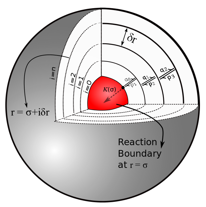
Employing this stochastic matrix on the system (3.15) yields the same result as in the spherical random walk except for the first equation in the boundary $r_{0}$ which yields,

$$\pi_{0} {}^{t+1}=\pi_{0}^{t}+\frac{\delta tD}{\delta r^{2}}\left[\pi_{1}^{t}-2\pi_{0}^{t}+\pi_{0}^{t}\left(1-\frac{\delta r^{2}}{D}\frac{\kappa}{4\pi r_{0}^{2}\delta r}\right)\right]-\delta t\left[\frac{D}{r_{0}}\frac{\pi_{1}^{t}}{\delta r}+\frac{D}{\delta r}\left(\frac{\pi_{0}^{t}}{r_{0}+\delta r}\right)\right].$$

$$\Rightarrow\ \ \ \pi_{0} {}^{t+1}=\pi_{0}^{t}+\delta tD\left[\frac{\pi_{1}^{t}-2\pi_{0}^{t}+\pi_{-1}^{t}}{\delta r^{2}}\right]-\delta t\frac{2D}{r_{0}}\left[\frac{\pi_{1}^{t}-\pi_{-1}^{t}}{2\delta r}\right]+\delta t\frac{D}{\delta r}\left[\frac{\pi_{0}^{t}}{r_{0}-\delta r}-\frac{\pi_{0}^{t}}{r_{0}+\delta r}\right],$$

where $\pi_{-1}^{t}$ satisfies

$$\pi_{0}^{t}-\frac{\delta r\kappa}{4\pi Dr_{0}^{2}}\pi_{0}^{t}=\pi_{-1}^{t}+\delta r\frac{\pi_{0}^{t}}{r_{-1}}+\delta r\frac{\pi_{-1}^{t}}{r_{0}}$$ (3.25)

Dividing by $\delta r$ and taking the limit as $\delta_{t}\rightarrow 0$, $\delta_{r}\rightarrow 0$ again satisfies the Fokker-Planck equation (Eq. 3.19) with second order accuracy in space; however, Eq. 3.25 now becomes

$$\left.\frac{\partial\Pi(r,t)}{\partial r}\right|_{r=\sigma}=\frac{\kappa}{4\pi\sigma^{2}D}\Pi(\sigma,t)+\frac{2\Pi(\sigma,t)}{\sigma}$$

with first order accuracy, where $\Pi(r,t)$ is the continuous analog of $\pi_{i}^{t}$. Employing once again the change of variables in Eq. 3.20, we recover the well known boundary condition of Collins and Kimball (see Eq. 1.6),

$$4\pi\sigma^{2}D\left.\frac{\partial f(r,t)}{\partial r}\right|_{r=\sigma}=\kappa f(\sigma,t).$$

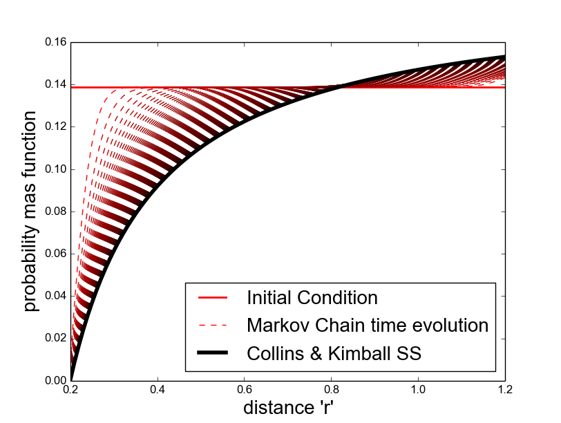
We would like to provide a comparison between Collins and Kimball solution (Eq. 1.7) and our Markov approach; however, our equations model the dynamics for the probability mass function and Collins and Kimball models the concentration gradient. A possible probabilistic interpretation of Collins and Kimball model is given by the Green,s function for an isolated pair, like in the GFRD approach [55, 65, 64]; however, the steady state will yield zero. The main difficulty in providing a better probabilistic interpretation is the far-field boundary condition with constant value at infinity. In order to address this issue, we will take an alternate approach to compare the steady state solution. We will solve the Fokker-Planck equation (Eq. 1.5a) with the boundary conditions,

$$\left.4\pi\sigma^{2}D\frac{\partial f(r,t)}{\partial r}\right|_{r=\sigma}=\left.4\pi R^{2}D\frac{\partial f(r,t)}{\partial r}\right|_{r=R}=\kappa f(\sigma,t),$$ (3.26)

and $\int_{\sigma}^{R}4\pi r^{2}f(r,t)dr=1$. These conditions mean that the probability flux at $r=\sigma$ is the same as the flux at $r=R$, which is, from a probabilistic point of view, a periodic boundary condition. The steady state solution is exactly of the same form as Eq. 1.7, but with a fixed constant $c_{0}=A_{0}$,

$$f_{ss}(r) = A_{0}\left[1-\frac{\kappa\sigma}{4\pi D\sigma+\kappa}\left(\frac{1}{r}\right)\right],$$ (3.27)

$$A_{0} = \left[4\pi\left(\frac{R^{3}-\sigma^{3}}{3}\right)-\frac{4\pi\sigma\kappa}{4\pi\sigma D+\kappa}\left(\frac{R^{2}-\sigma^{2}}{2}\right)\right]^{-1}.$$ (3.28)

This result provides a mathematical connection with the original gradient concentration approach and the probability approach. As a matter of fact, from a mathematical point of view, the boundary condition in Eq. 3.26 is also satisfied in the original Collins & Kimball formulation at steady state. In the probabilistic interpretation, the free parameter $A_{0}$ will give the normalization constant for the probability. In this case, we fixed it so the probability integrates to one. Nonetheless, we could have chosen it to integrate to any other value between $0$ and $1$. For instance, if we want the probability to integrate to $0.7$, we can obtain the corresponding value of $A_{0}$. In the concentration interpretation and scaled accordingly, this value will correspond to the concentration of the material/chemical bath in the far-field in order to get $30\%$ of absorbtion before reaching the steady state. For our current comparison and without loss of generality, we chose it so the probability integrates to one. Although this might seem odd given we have an absorbing boundary condition, the far-field boundary condition is a source compensates for the absorption.

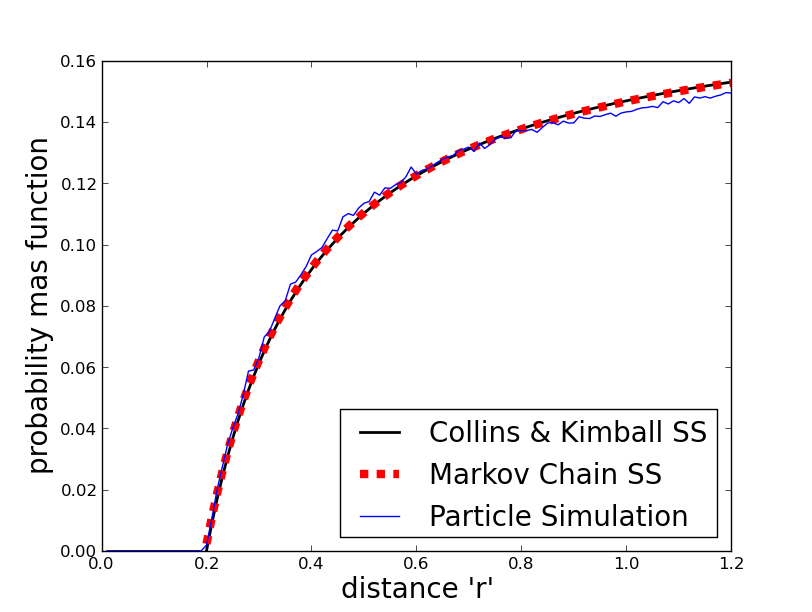
In order to do the comparison, we modify the stochastic matrix (3.24) in our Markov model to model this periodicity by adding a $\tilde{\kappa}(\sigma)\delta t$ term in the last column and first row of the truncated stochastic matrix. We can compute the probability mass function from the Markov chain at time $t=n\delta t$ with $\boldsymbol{\pi}^{n}=\boldsymbol{\pi}^{0}\mathbb{P}^{n}$ until reaching the steady state $\boldsymbol{\pi}^{ss}=\boldsymbol{\pi}^{ss}\mathbb{P}$, and we can also do a particle based simulation using the jump probabilities. A comparison of the three approaches for uniform initial distributions is shown in Figure 5. The quantity plotted in this and every other figure in this section is $\pi_{i}^{t}/(4\pi r_{i}^{2}\delta r)$, which uses the first order equation that the probability between the point-continuous and spherical-discrete setting is $\pi_{i}^{t}=4\pi r_{i}^{2}f(r_{i},t)\delta r$. Note the agreement between the ensemble behavior of stochastic trajectories and the probability mass function is expected from the stochastic theory. This stochastic formulation of our model is what allows trivial particle-based simulations that accurately match the expected statistical behavior given by probability mass function dynamics. It should also be noted this is an open system in non-equilibrium steady state (NESS) driven by the flux from the sink and source at the inner and outer boundary, so it will not satisfy detailed balance [44].

Figure 5: Model verification: (a) The steady state of Collins and Kimball’s solution of Eq. 1.7 (or Eq. 3.27) with $c_{0}=A_{0}$ from Eq. 3.28 is plotted with a thick black line. The initial condition (uniform distribution) for the discrete Markov model is plotted as an horizontal red line. The dashed lines represent the convergence in time to the steady state of the Markov chain from $t=0$ to $t=1$ taken every 100 time steps; the darker lines correspond to longer times. (b) The steady state of the periodic solution to Collins and Kimball (Eq. 3.27) is compared to the Markov chain steady state and to a particle based simulation with 3E6 particles and 1E4 time iterations. The parameters used were: $\delta r=0.01$, $\delta t=0.0001$, $D=0.1$, $\tilde{\kappa}(\sigma)=4000.0$, $\sigma=0.2$, and 100 shells for the discrete models.

In order to provide an even more complete connection to the meaning of the Collins and Kimball rate in the discrete model, consider a particle in the shell in the reaction boundary $r_{0}=\sigma$. The particle has three possible movements: it can diffuse to level $i=1$ with probability $q_{0}\approx\delta tD/\delta r^{2}$ (first order); it can react with probability $\tilde{\kappa}(\sigma)\delta_{t}$; or it can diffuse along the spherical shell with probability $\xi$. Lets assume that if the particle diffuses out to shell $n=1$ then the particle is fully dissociated without any geminate recombinations; therefore, the probability of reaction while diffusing in the shell $r_{0}$ is given by

$$\phi=\tilde{\kappa}(\sigma)\delta_{t}\sum_{n=0}^{\infty}\xi^{n}=\frac{\tilde{\kappa}(\sigma)\delta_{t}}{1-\xi}=\frac{\tilde{\kappa}(\sigma)\delta_{t}}{\tilde{\kappa}(\sigma)\delta_{t}+\delta tD/\delta r^{2}}$$

where we used that $1=\xi+\tilde{\kappa}(\sigma)\delta_{t}+q_{0}$. As we already obtained that $\tilde{\kappa}(r)=\kappa/(4\pi r^{2}\delta_{r})$, we can substitute $\tilde{\kappa}(\sigma)$, which yields

$$\phi=\frac{\kappa}{4\pi\sigma^{2}D/\delta_{r}+\kappa}.$$

This is the discrete approximation of the fraction of reactions due to geminations of the Collins and Kimball reaction rate [3, 8, 52]. Its continuous counterpart is shown in Eqs. 1.13 and 1.14. Note we do not expect convergence as $\delta r\rightarrow 0$, since this approximate derivation will no longer make sense from a continuous perspective. Nonetheless, it provides a clear physical picture of how the gemination process work.

3.3 Discrete model for reversible reaction-diffusion

In this section, we will extend the previous model to deal with reversible reactions. We will begin by adding one more state $\pi^{t}_{b}$ at the beginning of the state vector: $\boldsymbol{\pi}^{t}=\left[\pi^{t}_{b},\pi^{t}_{0},\pi^{t}_{1},\cdots,\pi^{t}_{i},\cdots\right]$. This new state means the probability of the $B$ molecule to be bound to $A$. The stochastic matrix will naturally require an additional first row and column

$$\mathbb{P}=\left[\begin{matrix}1-P_{u}&P_{u}&0&0&\cdots\\ P_{b}&1-(q_{0}+P_{b})&q_{0}&0&\cdots\\ 0&p_{1}&1-(p_{1}+q_{1})&q_{1}&\cdots\\ \vdots&&&\ddots&\end{matrix}\right],$$ (3.29)

where $P_{b}=\tilde{\kappa}(r)\delta t$ and $P_{u}=\tilde{\mu}(r_{0})\delta t$ is the probability for dissociation to occur at the corresponding shell. The dissociation parameter $\tilde{\mu}(r)$ is trivially related to the constant dissociation rate $\mu$ in Eq. 1.10 by $\tilde{\mu}(r)=\mu$ with units of time^-1. Once again $P_{b}$ and $P_{u}$ could be replaced with more accurate exponential expressions, see Appendix B.

Note that now all the rows of the stochastic matrix sum to zero since we are taking into account the particles that have already reacted. Also note $\pi^{t}_{b}$ is the probability of $B$ being bound to $A$, so it can be written as $\pi^{t}_{b}=[1-S_{d}(t)]$, where $S_{d}(t)=\sum_{i=0}^{N}\pi_{i}^{t}$ is the probability of being unbound at time $t$. The first equation now yields,

$$\pi_{b}^{t+1}=\pi_{b}^{t}\left[1-\tilde{\mu}(r_{0})\delta t\right]+\pi_{0}^{t}\tilde{\kappa}(r_{0})\delta t.$$

Dividing by $\delta r$ and taking the limit, we can arrange the left hand side to yield $\Pi_{b}(t)\approx(\pi_{b}^{t+1}-\pi_{b}^{t})/\delta t$. On the right hand side it might seem this equation might not converge, since $\tilde{\kappa}(r_{0})$ scale as $1/\delta r$. However, using Eq. 3.20 we know $\pi_{0}^{t}=4\pi r^{2}f(r_{0},t)\delta r$ at first order, so in the limit we immediately obtain,

$$\frac{df_{b}(t)}{dt}=\kappa f(r_{0},t)-\mu f_{b}(t),$$ (3.30)

where $f_{b}(t)=\Pi_{b}(t)$, so $\mu$ has units of time^-1 and $\kappa$ of volume over time as expected. This equation only involves reaction, since we didn’t allow any diffusion to happen when $B$ is in the bound state. The second equation will yield even more interesting results, the equation is

$$\pi_{0}^{t+1}=\pi_{0}^{t}+\frac{\delta tD}{\delta r^{2}}\left[\pi_{1}^{t}-2\pi_{0}^{t}+\pi_{0}^{t}\left(1-\frac{\delta r^{2}}{D}\frac{\kappa}{4\pi r_{0}^{2}\delta r}\right)\right]-\delta t\left[\frac{D}{r_{0}}\frac{\pi_{1}^{t}}{\delta r}+\frac{D}{\delta r}\left(\frac{\pi_{0}^{t}}{r_{0}+\delta r}\right)\right]+\delta t\mu\pi_{b}^{t}.$$

$$\Rightarrow\ \ \ \pi_{0}^{t+1}=\pi_{0}^{t}+\delta tD\left[\frac{\pi_{1}^{t}-2\pi_{0}^{t}+\pi_{-1}^{t}}{\delta r^{2}}\right]-\delta t\frac{2D}{r_{0}}\left[\frac{\pi_{1}^{t}-\pi_{-1}^{t}}{2\delta r}\right]+\delta t\frac{D}{\delta r}\left[\frac{\pi_{0}^{t}}{r_{0}-\delta r}-\frac{\pi_{0}^{t}}{r_{0}+\delta r}\right],$$

where $\pi_{-1}^{t}$ satisfies

$$\pi_{0}^{t}-\frac{\delta r\kappa}{4\pi Dr_{0}^{2}}\pi_{0}^{t}+\mu\frac{\delta r^{2}}{D}\pi_{b}^{t}=\pi_{-1}^{t}+\delta r\frac{\pi_{0}^{t}}{r_{-1}}+\delta r\frac{\pi_{-1}^{t}}{r_{0}}.$$ (3.31)

Dividing by $\delta r$ and taking the limit as $\delta_{t}\rightarrow 0$, $\delta_{r}\rightarrow 0$ again satisfies the Fokker-Planck equation (Eq. 3.19). For Eq. 3.31, we use again Eq. 3.20 and the fact that $\pi_{i}^{t}=4\pi r^{2}f(r_{i},t)\delta r$ at first order to obtain

$$4\pi\sigma^{2}D\left.\frac{\partial f(r,t)}{\partial r}\right|_{r=\sigma}=\kappa f(\sigma,t)-\mu f_{b}(t),$$

where $f_{b}(t)=\Pi_{b}(t)$ and $\sigma=r_{0}$. Now note that $f_{b}(t)=[1-S(t)]$, where $S(t)=\int_{\sigma}^{\infty}4\pi r^{2}f(r,t)dr$ is the probability of being unbound, i.e. the continuous version of $S_{d}(t)$, so we can write

$$4\pi\sigma^{2}D\left.\frac{\partial f(r,t)}{\partial r}\right|_{r=\sigma}=\kappa f(\sigma,t)-\mu[1-S(t)],$$ (3.32)

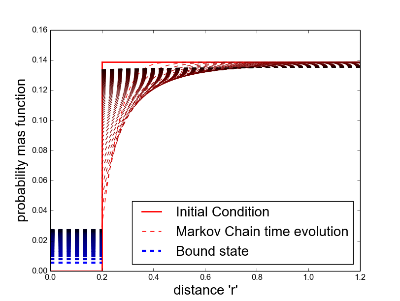
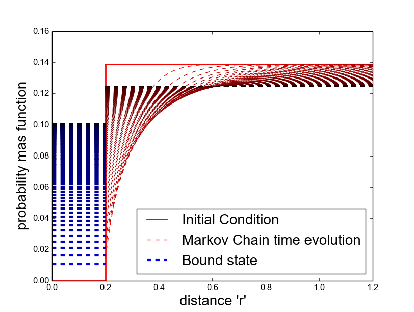
This is the back-reaction boundary condition (Eq. 1.10) found in the exact solution for the reversible reaction [1, 26, 40]. Note this boundary condition couples the Fokker-Planck equation (Eq. 3.19) with the Eq. 3.30. The probability of being unbound can be represented in terms of the integral in Eq. 1.11, which yields a non-local boundary condition and sheds light in the fact that some non-local boundary conditions might be only a condensed technique to write complicated coupled systems. The time evolution of the probability mass function given by our Markov approach is shown for two set of parameters in Figure 6. The initial condition is given as uniform for the unbound state and zero for the bound one. The probability is conserved following,

$$\pi_{b}^{t}+\sum_{i=0}^{N}\pi_{i}^{t}=1,$$

for all times $t$, where $\pi_{i}^{t}$ is equal to $4\pi r_{i}^{2}f(r_{i},t)\delta r$ at first order, and $\pi_{b}$ is the probability of being bound—its value is represented by the height of the blue dashed bar on the plots in Figure 6. On both plots we can observe convergence towards a flat steady state. As we included the bound state as part of the irreducible and aperiodic Markov chain as well as no-flux boundaires elsewhere, the system is closed and has a steady state, so detailed balance must be satisifed. The probability lost in the unbound region is balanced by the probability gained in the bound one. Since the model is a Markov chain, particle-based simulation of this discrete stochastic reversible diffusion-influenced model is trivial by employing the jump probabilities.

Figure 6: Convergence of the discrete model to steady state for the reversible case for two sets of parameters. The initial condition is a uniform distribution in the unbound state and zero on the bound state, and it is plotted as a red line. The dashed lines represent the convergence in time to the steady state of the Markov chain from $t=0$ to $t=1$ taken every 400 and 1000 time steps respectively; the darker lines correspond to longer times. (a) Parameters used were: $\delta r=0.01$, $\delta t=0.0001$, $D=0.1$, $\tilde{\kappa}(\sigma)=8000.0$, $\mu=200$ $\sigma=0.2$, and 100 shells. The bound state $\pi_{b}$ value at different time steps is shown as an horizontal line from $r=[0,\sigma]$ (b) Same parameters with rates exaggerated to better show the convergence to the steady state.

Note the continuous limit we just derived of the discrete model provides a more simple form of the model than the original back-reaction continuous model as two coupled partial/ordinary differential equations,

$$\frac{df_{b}(t)}{dt}=\kappa f(r_{0},t)-\mu f_{b}(t),$$ (3.33)

$$\frac{\partial f(r,t)}{\partial t}=\nabla\cdot[D(r)\nabla f(r,t)]$$ (3.34)

with the back-reaction boundary condition

$$4\pi\sigma^{2}D\left.\frac{\partial f(r,t)}{\partial r}\right|_{r=\sigma}=\kappa f(\sigma,t)-\underbrace{\mu f_{b}(t)}_{\text{$\mu[1-S(t|r_{0})]$}}.$$ (3.35)

Although this equation can be derived from the original model, we recovered it naturally from the discrete model limit. As the association and dissociation were intuitively implemented in the discrete model, its convergence to the original continuous model, provides additional validation that it is appropriate to model reversible bimolecular reactions via diffusion encounter. It should be mentioned a similar model was developed using a Master Equation to derive modified reaction rates for simulations of the reaction diffusion master equation (RDME) [16]. Nonetheless, the methodology follows a different logic; they assume the reaction rate in the Master Equation as unknown, and they use the continuous theory to derive an appropriate rate for some specific discretization. In our work, we chose fixed reaction probability, and we showed the condition under which this recovers the continuous theory. We also provide the parameters of the continuous model in terms of the discrete probabilities, which provides insight into the meaning of these quantities. In addition, the relation we obtained between the rate and the discretization parameters is simpler, and they don’t extend their model to the cases discussed in the following Sections.

3.4 Reversible reaction-diffusion with unbinding radius

In the previous model with reversible reaction, we assumed the $B$ particles are associated and dissociated in the same reaction shell corresponding to $r=\sigma$. However, the probability of reacting/dissociating can be distributed along different spatial points and not only on a specific boundary. In the stochastic matrix (3.29), the term $P_{u}$ can be placed in any of the columns in the first row. For instance, if this term is collocated in the $n^{th}$ column of the matrix, when the $B$ molecule is dissociated, it would be placed in the sphere $i=n$ with unbinding radius $\sigma_{u}=\sigma+n\delta r$ (see Figure 4). The binding process occurs in the boundary $i=0$ with $r=\sigma$, so we could say there is a binding radius $r=\sigma$ and an unbinding radius at $r=\sigma_{u}$. A new question now arises: if we consider an ensemble of these systems at thermodynamic equilibrium, is detailed balance satisfied?

Figure 7: Convergence of the discrete model to its steady state for the reversible case with an unbinding radius. The initial condition is a uniform distribution in the unbound state and zero on the bound state, and it is plotted as a red line. The dashed lines represent the convergence in time to the steady state of the Markov chain from $t=0$ to $t=1$ taken every 100 time steps; the darker lines correspond to longer times. (a) Parameters used were: $\delta r=0.01$, $\delta t=0.0001$, $D=0.1$, $\tilde{\kappa}(\sigma)=6000.0$, $\mu=50$, $\sigma=0.2$, $\sigma_{u}=0.7$, and 100 shells. The bound state $\pi_{b}$ value at different time steps is shown as an horizontal dashed line from $r=[0,\sigma]$. The final steady state is emphasized as a black continuous curve; as the slope from the right of $r=\sigma_{u}$ is zero, we know the net flux for $r>\sigma_{u}$ is zero, as expected. Detailed balance is not satisfied between $r=\sigma$ and $r=\sigma_{u}$

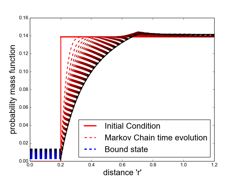
Detailed balance tells us that in a chemical kinetic system at equilibrium every elementary reaction is balanced by its reverse reaction $\pi_{i}P_{i\rightarrow j}=\pi_{j}P_{j\rightarrow i}$ [32], where $P_{a\rightarrow b}$ is the transition probability from state $a$ to $b$. At equilibrium, detailed balanced will not be satisfied inside the shells $i=0$ and $i=n$ since we have an open system with a source and a sink. In these shells, we actually observe a NESS, like the one from Section 3.2. Nonetheless, we scaled the unbinding rate so the net flux coming out of shell $i=n$ is zero, so detailed balance will be satisfied everywhere else between shell $i=n$ and the outermost shell. This might seem at first confusing since detailed balance is based on chemical kinetics; however, the concept can be easily extended to diffusion and random walks. As we know that as long as there are no flux conditions in the boundaries of a system in steady state, detailed balance must be satisfied everywhere. As there is no flux condition at shell $i=n$ and at infinity (or at the outermost shell), detailed balance is satisfied between those two boundaries. This is indeed the reason why the particle-based stochastic reaction-diffusion algorithms that introduce an unbinding radius work. Introducing the unbinding radius sacrifices accuracy in the local region around $r=\sigma$, but it allows fast and accurate simulations [3, 11] on slightly larger scales. In Figure 7, we can observe the time convergence of the probability mass function to the steady stated for this case. In contrast with Figure 6, we can see between $r=\sigma$ and $r=\sigma_{u}$ the solution has non-zero flux; this is the region where detailed balance will not be satisfied. However, the solution will be accurate everywhere else, where detailed balance is satisfied.

3.5 Radial random walk with spherical symmetry under a potential

Assuming the random walk is influenced by a smooth interaction potential $U(r)$, we can modify the original transition probabilities in Eq. 3.17 by including the interaction potential term as

$$\begin{split}p_{i}=\delta t\left(\frac{D}{\delta r^{2}}-\frac{D}{r_{i-1}\delta r}+\frac{\beta D}{4\delta r^{2}}\left[U_{i+1}-U_{i-1}\right]\right),\\ q_{i}=\delta t\left(\frac{D}{\delta r^{2}}+\frac{D}{r_{i+1}\delta r}-\frac{\beta D}{4\delta r^{2}}\left[U_{i+1}-U_{i-1}\right]\right),\end{split}$$ (3.36)

where $\beta=1/k_{B}T$, with $k_{B}$ the Boltzmann constant and $T$ the temperature. With these new values of $p_{i}$ and $q_{i}$ in the matrix 3.24, we can rewrite the $i^{\mathrm{th}}$ equation of (3.15) as,

$$\pi_{i} {}^{t+1}=\pi_{i}^{t}+\delta tD\left[\frac{\pi_{i-1}^{t}-2\pi_{i}^{t}+\pi_{i+1}^{t}}{\delta r^{2}}\right]-\delta t\frac{2D}{r_{i}}\left[\frac{\pi_{i+1}^{t}-\pi_{i-1}^{t}}{2\delta r}\right]$$

$$+\delta t\frac{D}{\delta r}\left[\frac{\pi_{i}^{t}}{r_{i}-\delta r}-\frac{\pi_{i}^{t}}{r_{i}+\delta r}\right]+\delta t\frac{\beta D}{2\delta r}\left[\pi_{i+1}^{t}\left(\frac{U_{i+2}-U_{i}}{2\delta r}\right)-\pi_{i-1}^{t}\left(\frac{U_{i}-U_{i-2}}{2\delta r}\right)\right].$$ (3.37)

Dividing by $\delta r$ and taking the limit as before we obtain

$$\frac{\partial\Pi(r,t)}{\partial t}=D\frac{\partial^{2}\Pi(r,t)}{\partial r^{2}}-\frac{\partial}{\partial r}\left(\frac{2D}{r}\Pi(r,t)\right)+\beta D\frac{\partial}{\partial r}\left[\Pi(r,t)\frac{\partial U(r)}{\partial r}\right],$$ (3.38)

with second order accuracy in space. Employing once again the fact that $\Pi(r,t)=4\pi r^{2}f(r,t)$, we recover the Smoluchowski equation under a potential [56],

$$\frac{\partial f(r,t)}{\partial t} =\frac{D}{r^{2}}\frac{\partial}{\partial r}\left(r^{2}\left[\frac{\partial f(r,t)}{\partial r}+\beta f(r,t)\frac{\partial U(r)}{\partial r}\right]\right)$$ (3.39)

$$=\frac{D}{r^{2}}\frac{\partial}{\partial r}\left(r^{2}e^{-\beta U(r)}\frac{\partial}{\partial r}e^{\beta U(r)}f(r,t)\right).$$ (3.40)

We have not talked about the boundary yet. This will be a very subtle issue as we will comment on further. For the time being, lets assume the boundary is given as that of the matrix (3.24). In such case the first difference equation of the Kolmogorov forward equation yields,

$$\pi_{0}^{t+1}= \pi_{0}^{t}+\frac{\delta tD}{\delta r^{2}}\left[\pi_{1}^{t}-2\pi_{0}^{t}+\pi_{0}^{t}\left(1-\frac{\delta r^{2}}{D}\frac{\kappa}{4\pi r_{0}^{2}\delta r}\right)\right]-\delta t\left[\frac{D}{r_{0}}\frac{\pi_{1}^{t}}{\delta r}+\frac{D}{\delta r}\left(\frac{\pi_{0}^{t}}{r_{0}+\delta r}\right)\right]+$$

$$\frac{\delta t\beta D}{2\delta r}\left[\pi_{1}^{t}\left(\frac{U_{2}-U_{0}}{2\delta r}\right)+\pi_{0}^{t}\left(\frac{U_{1}-U_{-1}}{2\delta r}\right)\right].$$

Once again, in order to find the boudary condition, we rewrite this equation in the same form than Eq. 3.37 by introducing the ghost cell $\pi_{-1}^{t+1}$. This will require introducing values for the potential at two ghost cells $U_{-1}$ and $U_{-2}$,

$$\pi_{0}^{t+1}= \pi_{0}^{t}+\delta tD\left[\frac{\pi_{1}^{t}-2\pi_{0}^{t}+\pi_{-1}^{t}}{\delta r^{2}}\right]-\delta t\frac{2D}{r_{0}}\left[\frac{\pi_{1}^{t}-\pi_{-1}^{t}}{2\delta r}\right]+\delta t\frac{D}{\delta r}\left[\frac{\pi_{0}^{t}}{r_{0}-\delta r}-\frac{\pi_{0}^{t}}{r_{0}+\delta r}\right]+$$

$$\delta t\frac{\beta D}{2\delta r}\left[\pi_{1}^{t}\left(\frac{U_{2}-U_{0}}{2\delta r}\right)-\pi_{-1}^{t}\left(\frac{U_{0}-U_{-2}}{2\delta r}\right)\right],$$

where $U_{-1}$ and $U_{-2}$ are usually well defined since the boundary where $i=0$ corresponds to $\sigma>0$ and $\delta r$ is small. In the case where these are undefined, we can always use articial values to match the right derivative and curvature of the potential at the boundary. This equation divided by $\delta r$ in the limit $\delta_{t}\rightarrow 0$ and $\delta_{r}\rightarrow 0$ is again reduced to the appropriate Fokker-Planck equation, given by Eq. 3.38. However, analogously as before, $\pi_{-1}^{t}$ needs to satisfy,

$$\pi_{0}^{t}-\frac{\delta r\kappa}{4\pi Dr_{0}^{2}}\pi_{0}^{t}+\frac{\beta}{4}\pi_{0}^{t}(U_{1}-U_{-1})=\pi_{-1}^{t}+\delta r\frac{\pi_{0}^{t}}{r_{-1}}+\delta r\frac{\pi_{-1}^{t}}{r_{0}}-\frac{\beta}{4}\pi_{-1}^{t}(U_{0}-U_{-2}),$$

which in the continuous limit becomes

$$\left.\frac{\partial\Pi(r,t)}{\partial r}\right|_{r=\sigma}=\frac{\kappa}{4\pi\sigma^{2}D}\Pi(\sigma,t)+\frac{2\Pi(\sigma,t)}{\sigma}-\beta\left.\frac{\partial U(r)}{\partial r}\right|_{r=\sigma}\Pi(r,t),$$

with first order accuracy in space. Using again Eq. 3.20, we can rewrite it as

$$4\pi\sigma^{2}D\left.\frac{\partial f(r,t)}{\partial r}\right|_{r=\sigma}=\kappa f(\sigma,t)-4\pi\sigma^{2}D\beta\left.\frac{\partial U(r)}{\partial r}\right|_{r=\sigma}f(\sigma,t)$$

$$\Rightarrow\ \ \ 4\pi\sigma^{2}De^{-\beta U(\sigma)}\left[\frac{\partial e^{\beta U(r)}f(r,t)}{\partial r}\right]_{r=\sigma}=\kappa f(\sigma,t),$$

which is the Collins-Kimball-Debye boundary condition [53]. If we would have used matrix (3.29) instead, we would have obtained the back-reaction boundary condition in Eq. 3.32 with the addition of the potential factors. However, there is the subtlety of how to define the bound state that we discussed in Section 2.2. Does it depend on the distance between $A$ and $B$ molecules, or does it depend on the state? According to our previous discussion, it will depend on the physical problem at task.

Figure 8: Convergence to steady state for the diffusion under a force field case for two potentials. The initial condition for the discrete Markov model, which is a uniform distribution, is plotted as a thick red line. The thin lines represent the convergence in time to the steady state of the Markov chain from $t=0$ to $t=0.2$ taken every 10 time steps; the darker lines correspond to longer times. (a) Plot using potential $U_{(r)}=U_{K}(r)$. The parameters used were $V_{0}=0.0001$, $r_{m}=0.5$, $A=2.0$, $\delta r=0.01$, $\delta t=0.0001$, $D=0.1$, 100 shells and $r_{0}=0$.(b) Plot using a Lennard-Jonnes type potential $U(r)=U_{LJ}(r)$. The parameters were $V_{0}=0.00005$, $r_{m}=0.22$ $\delta r=0.002$, $\delta t=2E-5$, $D=0.1$, 500 shells and $r_{0}=0.2$.

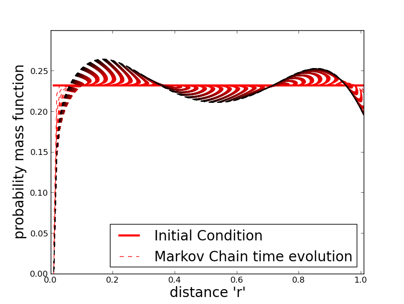
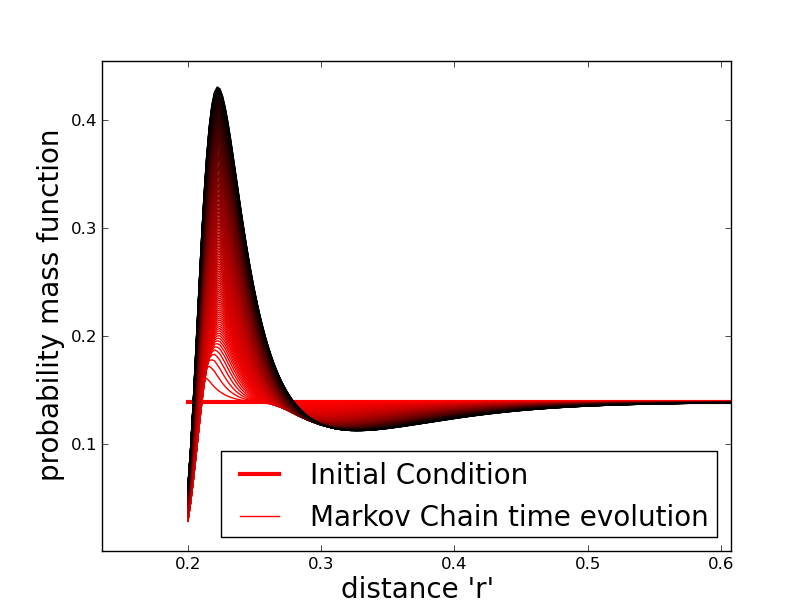
In Figure 8, we plot the convergence to the steady state for the two potential functions,

$$U_{K}(r) =V_{0}\left[(A(r-r_{m}))^{4}-(A(r-r_{m}))^{2}\right],\hskip 14.22636pt\mathrm{and}$$

$$U_{LJ}(r) =V_{0}\left[\left(\frac{r_{m}}{r}\right)^{12}-2\left(\frac{r_{m}}{r}\right)^{6}\right].$$

These correspond to the potential in Kramers original work and a Lennard-Jonnes potential. We observe the steady state distribution exhibits bistability, even when using the Lennard-Jonnes potential due to the geometrical drift. In this case, the reversible reaction can be modeled without the need of a boundary, and the state of $B$ can be stated as bound or unbound depending on which side of the separatrix of the potential it is. Note this still matches both the distance and state definition mentioned in Section 2.2. However, if the potential doesn’t only depend on $r$ but on more variables, the distance and state definition might not provide the same answer.

Once again, as we have a steady state and zero flux boundaries, detailed balance must be satisfied, and the equilibrium state satisfies the Gibbs-Boltzmann distribution. We should also mention an alternative discretization for discontinuous potentials was introduced in [67]. Their discretization is only performed in one dimension and does not implement reversible reacting boundaries. In the future, it would be interesting to explore how to extended their to include reversible reaction boundaries. Another very relevant work was done in [28, 37], where a similar discretization as a Markov chain is given; however, the emphasis is on providing a numerical solution of the Smoluchowski equation instead of a stochastic framework that allows particle based simulations in conjunction with probability mass function dynamics.

3.6 Extension to multiple molecules

The aim of the present work is to unify theories and algorithms and to provide a deeper understanding of stochastic reaction-diffusion processes, by using a simple intuitive model. Nonetheless, we will offer some suggestions on its value in computations, in particular, its extension to multiple-molecule simulations. One of the key advantages of this formulation, in comparison to other algorithms, is that it can handle multiple $B$’s in particle-based simulations naturally on the same grid, and it doesn’t need to decouple a system into multiple two-body problems. Of course, once a $B$ has been absorbed a new $B$ cannot be absorbed until the previous one is dissociated. In this sense, our model already handles multiple molecules.

The real challenge is when one also has multiple $A$’s. If we assume $A$’s are diluted macromolecules, there are several possibilities to extend this model that would be worthwhile to explore. One possibility is to create non-overlapping truncated spherical grids around each $A$ molecule. Each one of this molecules diffuses along with its grid following a random walk with diffusion coefficient $D_{A}$. In the same manner, $B$ molecules diffuse on open space following a random walk with coefficient $D_{B}$, unless they diffuse into one of the outermost spherical shells or if they are already inside one. If a $B$ molecule diffuses into one of the outer shells, it will undergo diffusion inside the spherical shells following the model from the previous sections. If the molecule escapes the outermost shell of the grid, it will return to diffuse freely with the direction of exit chosen randomly from a uniform distribution. Complications will arise if at some time step two grids of $A$ overlap. In this case, we would need to calculate new non-overlapping grids for the two $A$’s, which will force a smaller time step. However, as $A$ is dilute this should not happen very often. In the case where $A$ molecules are binding sites fixed in space, this could be an efficient and accurate approach.

Another possible implementation is to precompute the probability distribution function in a large and high-resolution grid and save these into a lookup table. The table could then be used as the reference solution to compute the probabilities in simulation algorithms like eGFRD or FPKMC. The difference is that this solution uses the back-reaction boundary condition and not the partially absorbing one. This could speed up existing algorithms since the partially absorbing boundary requires modeling every dissociation event while the back-reaction boundary does not. This model provides an easy and intuitive alternative to compute lookup tables for third-parties interested in developing their own simulations, and it also encourages reproducibility. It would be interesting to compare the lookup tables obtained in our discrete model with those of other simulation packages. Implementation of these extensions and the comparison studies between different algorithms is left as future work.

4 Discussion

We developed a discrete time/space stochastic model for bimolecular chemical reaction via diffusion encounter. The model converges to all the well known classical results of continuous irreversible diffusion-influenced reaction theory. It also allows diffusion under a force field, like in the theories of Debye and Kramers.

The significance of this formulation is for the case of reversible reactions, where there have been extensive discussions on the best approach to model the process. One of the main models is given by the usual diffusion equation, Eq. 1.9a, coupled with the back-reaction boundary condition from Eq. 3.32. The main issue with this model, however, is that the back-reaction boundary condition is so complicated that it obscures the underlying stochastic process and consequently an accurate and transparent particle-based simulation. The discrete model presented in the present paper was inherently constructed as a stochastic process using simple notions of discrete association and dissociation reactions. In the continuous limit, it recovers the reversible diffusion-influenced theory, providing a clear description of the underlying stochastic process, which is hard to grasp in the continuous limit due to the nature of PRBM as shown in the Appendix B. In addition, it provides the continuous model parameters as a function of the jump and reaction probabilites, which elucidates the probabilistic interpretation of the parameters in the classical theory. It also allows straightforward simple Markovian algorithms to compute particle-based simulations and to compute the probability distribution, ensuring consistency between the two as well as conservation of probability.

In the continuous limit, we recover a more extensive version of the original back-reaction model, as in the Eqs. 3.33, 3.34 and 3.35. This result unifies the back-reaction boundary approach for reversible diffusion-influenced reactions with our discrete model. Furthermore, as we modeled the dissociation process following an exponential waiting time, the previous result also shows consistency between the reversible diffusion-influenced reaction theory and the approaches taken by other simulation algorithms, like eGFRD and FPKMC [58, 13].

The model also allows an immediate implementation of an unbinding radius for the dissociation process, and it provides the correct scaling for the dissociation rate in terms of the diffusion controlled association rate. This approach can be used by other simulation algorithms to speed up simulations in a similar manner as done in Smoldyn [3]. However, high accuracy and detailed balance are lost in the region inside the unbinding radius.

One disadvantage is the high accuracy of the discrete model causes numerical computations to be slow. Additionally, the model currently only works for one $A$ and one or multiple $B$’s; however, we provided a guideline for possible implementations with multiple $A$’s. These are left as future work. Other future directions are to implement extensions for volume reactivity models [12] and more complicated scenarios where a reaction is not only weighted as a function of space but also other variables. Regardless of its computation capabilities, the model itself provides a lot of insight on the modeling of reversible reactions, and it unifies different approaches by providing an underlying common stochastic framework. The discrete stochastic nature of this model establishes a research guideline that could lead to more robust computational solutions of complex models, where else continuous models might become increasingly convoluted, obscure or even intractable.

Appendix A Second order accuracy in no-flux boundaries

In the discretization of Section 3.1, we mentioned that we have second order accuracy in all the inner points. However, the boundary condition we obtain from Eq. 3.22 is only first order accurate. Lets check this, substracting Eq. 3.22 from $\pi_{0}^{t}$ and dividing by $\delta r$ we obtain,

$$\frac{\pi_{0}^{t}-\pi_{-1}^{t}}{\delta r} =\pi_{0}^{t}\frac{1}{\delta r}\left[1-\frac{\left(\frac{1}{\delta r}-\frac{1}{r_{-1}}\right)}{\left(\frac{1}{r_{0}}+\frac{1}{\delta r}\right)}\right]=\frac{\pi_{0}^{t}}{r_{0}^{2}}\frac{2r_{0}-\delta r}{1-\left(\delta r/r_{0}\right)^{2}}$$

$$=\pi_{0}^{t}\frac{2r_{0}-\delta r}{r_{0}^{2}}\sum_{i=0}^{\infty}\left(\frac{\delta r}{r_{0}}\right)^{2i}=\frac{2\pi_{0}^{t}}{r_{0}}\left[1+O(\delta r)\right].$$

Following standard finite difference theory [31], we take the limit as $\delta r\rightarrow 0$ and recover the zero flux boundary condition $\left.\frac{\partial\Pi(r,t)}{\partial r}\right|_{r=r_{0}}=\frac{2\Pi(r_{0},t)}{r_{0}}$ to first order. In general, this would not be desirable when discretizing a partial differential equation for simulation since the first order error would be propagated to the rest of the solution. Nonetheless, it is not clear how relevant the accuracy at the boundaries is when interpreting the discretization as jump probabilities in a Markov chain. Once again, the actual stochastic process is very clear in the discrete scenario since we are modeling a discrete stochastic process instead of the discretization of a continuous stochastic process. We also know that the reactions and the no-flux boundaries are modeled appropriately in the discrete process. How relevant is that we recover the continuous version of the boundary conditions with high accuracy is up for debate. The important part is that we do recover them showing consistency between the discrete and continuous models. In theory, we could try to modify the rates to obtain a second order discretization. However, it seems it would not be possible to write this discretization as a Markov chain anymore.

In the case of no-flux boundary conditions, there is an alternative approach that will yield second order accuracy. Lets concentrate on the steady state $\mathbf{\pi}^{ss}$, which we know satisfies detailed balance in the boundary $\pi_{0}^{ss}q_{0}=\pi_{1}^{ss}p_{1}$. The detailed balance condition for the problem in Section 3.1 can be written as,

$$\pi_{0}^{ss}\left(\frac{1}{r_{0}}+\frac{1}{\delta r}\right)=\pi_{1}^{ss}\left(\frac{1}{\delta r}-\frac{1}{r_{-1}}\right).$$ (A.1)

Substracting Eq. 3.22 from $\pi_{1}^{ss}$ and dividing the result by $2\delta r$, we obtain

$$\frac{\pi_{1}^{ss}-\pi_{-1}^{ss}}{2\delta r}=\frac{1}{2\delta r}\left[\pi_{1}^{ss}-\pi_{0}^{ss}\frac{\left(\frac{1}{\delta r}-\frac{1}{r_{-1}}\right)}{\left(\frac{1}{r_{0}}+\frac{1}{\delta r}\right)}\right].$$

Using the detailed balance condition of Eq. A.1, we can write the right hand side in terms of $\pi_{0}^{ss}$, which yields

$$\frac{\pi_{1}^{ss}-\pi_{-1}^{ss}}{2\delta r} =\frac{\pi_{0}^{ss}}{2\delta r}\left[\frac{\left(\frac{1}{\delta r}+\frac{1}{r_{1}}\right)}{\left(\frac{1}{\delta r}-\frac{1}{r_{0}}\right)}-\frac{\left(\frac{1}{\delta r}-\frac{1}{r_{-1}}\right)}{\left(\frac{1}{r_{0}}+\frac{1}{\delta r}\right)}\right]$$

$$=\frac{2r_{0}\pi_{0}^{ss}}{r_{0}^{2}-\delta r^{2}}=\frac{2\pi_{0}^{ss}}{r_{0}}\sum_{i=0}^{\infty}\left(\frac{\delta r}{r_{0}}\right)^{2i}=\frac{2\pi_{0}^{ss}}{r_{0}}\left[1+O(\delta r^{2})\right].$$

In the limit $\delta r\rightarrow 0$, it satisfies the no flux boundary condition with second order accuracy. This result is a consequence of the fact that our discretization can be interpreted as a Markov chain with detailed balance. The downsides are that this level of accuracy is only attained in the steady state solution and that it is not applicable for reactive boundaries.

Appendix B Partially reflected Brownian Motion (PRBM) as a limit of a random walk

Consider a random walk moving in one dimensional space. This can be described as a discrete time Markov chain, where the state $i$ refers to its position $x_{i}=i\delta x$. Let the probability of jumping from state $i$ to $i+1$ be $q_{i}$ and from state $i$ to $i-1$ be $p_{i}$, such that $p_{i}+q_{i}\leq 1$ and $1-(p_{i}+q_{i})$ is the probability of not jumping. For a purely reflective boundary at $i=0$, the only possibility is that the probability from jumping from state $i=0$ to the absorbed state is $p_{0}=0$. Analogously, for the purely absorbing boundary at $i=0$, it is required that $p_{0}=1$. In the same manner, we can easily think of the partially absorbing boundary condition at $i=0$, where the probability of being absorbed is $p_{0}=\epsilon$, with $\epsilon\in(0,1)$.

In order to study this random walk, lets assume $\delta x$ is fixed, so in order to satisfy that $p_{i}+q_{i}\leq 1$, we need $\delta t\leq\delta x^{2}/(2D)$. We would like to relate this random walk to Brownian Motion, so we need to assign correct values to $q_{i}$ and $p_{i}$. This is analogous to what we did in Section 3. The jump probabilities elsewhere outside the boundary should be $q_{i}=p_{i}=D\delta t/\delta x^{2}$. Following the same structure of the Markov chain from Eq. 3.15 with Eq. 3.24, the $i^{th}$ equation yields

$$\frac{\pi_{i}^{n+1}-\pi_{i}^{n}}{\delta t}=D\left[\frac{\pi_{i+1}^{n}-2\pi_{i}^{n}+\pi_{i-1}^{n}}{\delta x^{2}}\right],$$ (B.1)

which in the continuous limit recovers the one dimensional Brownian Motion $\partial\Pi/\partial x=D\partial^{2}\Pi/\partial x^{2}$. We also would like to recover the partially absorbing boundary condition, so we write the first equation in the Markov chain,

$$\frac{\pi_{0}^{n+1}-\pi_{0}^{n}}{\delta t}=\frac{D}{\delta x^{2}}\pi_{1}^{n}-\frac{D}{\delta x^{2}}\pi_{0}^{n}-\frac{\epsilon}{\delta t}\pi_{0}^{n},$$

where we used that the probability of staying at shell $i=0$ is $1-(q_{0}+p_{0})=1-(D\delta t/\delta x^{2}+\epsilon)$. In order for this equation to have the same form as Eq. B.1, we need to introduce the ghost shell $\pi_{-1}$ (as explained in Section 3.1), which satisfies

$$\epsilon\pi_{0}^{n}=D\delta t\frac{\pi_{0}^{n}-\pi_{-1}^{n}}{\delta x^{2}}.$$

In order to be able to recover the partially absorbing boundary condition $D\partial\Pi/\partial x|_{x=x_{0}}=\kappa\Pi(x_{0},t)$, we need to set $\epsilon=\kappa\delta t/\delta x$. It is now straightforward to write $\kappa$ and the Diffusion coefficient in terms of the jump probabilities in the discrete model by summing $p_{i}$ and $q_{i}$,

$$D=\frac{\delta x^{2}}{2\delta t},\hskip 14.22636pt\kappa=\frac{\delta x}{\delta t}\epsilon.$$ (B.2)

Note $\epsilon=0$ corresponds to a purely reflective boundary, which means $\kappa=0$, so $\partial\Pi/\partial x|_{x=x_{0}}=0$. The purely absorbing boundary corresponds to $\epsilon\rightarrow 1$. As shown in Section 3.1, $\delta t\leq\delta x^{2}/(2D)$, so $\kappa=\delta x\epsilon/\delta t\geq 2D\epsilon/\delta x$. Then, as $\delta x\rightarrow 0\Rightarrow\kappa\rightarrow\infty$, and the boundary condition becomes $\Pi(x_{0},t)=0$. As expected, this matches the limiting behavior from Collins and Kimball’s original work [10].

A very subtle issue is in the continuous limit of the probability of partial absorption $\epsilon=\kappa\delta t/\delta x$ with $\kappa$ constant. Again as $\delta t\leq\delta x^{2}/(2D)$, then $\epsilon\leq\kappa\delta x/(2D)$. This means that in the continuous limit $\delta x\rightarrow 0$, the probability of partial absorption goes to zero, $\epsilon\rightarrow 0$. However, $\epsilon=0$ means a purely reflective boundary, not a partially absorbing one, so the continuous limit of partially absorbing boundaries can be confusing, especially when trying to interpret them in particle-based simulations. The works [19, 9] elaborate on this issue and state that partially reflected Brownian Motion (PRBM) should be understood as purely reflective Brownian Motion conditioned to stop at a random moment given in terms of the local time process. In more intuitive terms, given a counting process $\mathcal{L}_{t}$ that counts the number of hits of a particle to the reflective boundary, the particle is killed (absorbed) when $\mathcal{L}_{t}\geq\chi$, where $\chi$ is an independent exponentially distributed random variable. It is in this sense that PRBM is best understood as the limit of a random walk. Furthermore, the parameters $D$ and $\kappa$ have a clear interpretation in terms of the jump and partial absorption probabilities. This result provides a more insightful understanding of the parameters even in the continuous model.

Also note the probability of absorption is a function of $\delta t$, $\epsilon=\kappa\delta t/\delta x$. Assuming we chose the largest possible value of $\delta t=\delta x^{2}/(2D)$, we have $\epsilon=\kappa\delta x/(2D)$. However, the fact that $0\leq\epsilon\leq 1$ limits our choice of $\delta x$. This bring into light that this choice of $\epsilon$ might not be the most appropriate one for a Markovian model. On the other hand, the probability $\epsilon=\kappa\delta t/\delta x$ could be understood as a first order approximation when sampling from an exponential waiting time,

$$1-e^{-\kappa\frac{\delta t}{\delta x}}\approx\kappa\frac{\delta t}{\delta x}.$$ (B.3)

This is basically emphasizing the fact that the reaction process at the boundary is Poissonian. Using $\epsilon=1-e^{-\kappa\delta t/\delta x}$ allows a more accurate choice for the discrete partial reaction probability since it always satisfy $0\leq\epsilon\leq 1$. In this case, the discrete parameter $\kappa$ is given by $\kappa=-\frac{\delta x}{\delta t}\log{[1-\epsilon]}$. It also gives the upper bound for the $\kappa$ parameter in a given discretization of the diffusion process. As $p_{0}+q_{0}\leq 1$, then $\epsilon+D\delta t/\delta x^{2}\leq 1$, so $\kappa\leq-\frac{\delta x}{\delta t}\log\left[D\frac{\delta t}{\delta x^{2}}\right]$; the equality corresponds to the purely absorbing case. Note that using the result from Eq. B.3 in the Markov model does not affect any of the previous limiting results. As a matter of fact, all the models in Section 3 can use this result without affecting the continuous limit behavior. It should also be noted this result would have never been obtained by looking for an accurate discretization of the continuous models; it is only obtained by looking for consistency with the underlying stochastic process.

References

- [1] N. Agmon. Diffusion with back reaction. J. Chem. Phys., 81(6):2811–2817, 1984.
- [2] N. Agmon and A. Szabo. Theory of reversible diffusion-influenced reactions. J. Chem. Phys., 92(9):5270–5284, 1990.
- [3] S. S. Andrews and D. Bray. Stochastic simulation of chemical reactions with spatial resolution and single molecule detail. Phys. Biol., 1(3):137, 2004.
- [4] P. Ao, C. Kwon, and H. Qian. On the existence of potential landscape in the evolution of complex systems. Complexity, 12:19–27, 2007.
- [5] L. Arnold. On the consistency of the mathematical models of chemical reactions. In Dynamics of synergetic systems, pages 107–118. Springer, 1980.
- [6] T. M. Bartol Jr, B. Land, E. E. Salpeter, and M. M. Salpeter. Monte Carlo simulation of miniature endplate current generation in the vertebrate neuromuscular junction. Biophys. J., 59(6):1290, 1991.
- [7] A. Batakis and V. H. Nguyen. On the Exit Distribution of Partially Reflected Brownian Motion in Planar Domains. Potential Anal., 38:537–548, 2013.
- [8] O. G. Berg. On Diffusion-Controlled Dissociation. Chem. Phys., 31(1):47–57, 1978.
- [9] K. Burdzy, Z.-Q. Chen, et al. Discrete approximations to reflected Brownian motion. Ann. Probab., 36(2):698–727, 2008.
- [10] F. C. Collins and G. E. Kimball. Diffusion-Controlled Reaction Rates. J. Colloid Sci., 4(4):425–437, 1949.
- [11] M. J. Del Razo, W. Pan, H. Qian, and G. Lin. Fluorescence Correlation Spectroscopy and Nonlinear Stochastic Reaction–Diffusion. The Journal of Physical Chemistry B, 118(25):7037–7046, 2014.
- [12] M. Doi. Stochastic theory of diffusion-controlled reaction. J. Phys. A: Math. Gen., 9(9):1479, 1976.
- [13] A. Donev, V. V. Bulatov, T. Oppelstrup, G. H. Gilmer, B. Sadigh, and M. H. Kalos. A first-passage kinetic Monte Carlo algorithm for complex diffusion–reaction systems. J. Comput. Phys., 229(9):3214–3236, 2010.
- [14] B. Drawert, S. Engblom, and A. Hellander. URDME: a modular framework for stochastic simulation of reaction-transport processes in complex geometries. BMC Syst. Biol., 6(1):76, 2012.
- [15] A. Einstein. Investigations on the Theory of the Brownian Movement. Courier Dover Publications, 1956.
- [16] D. Fange, O. G. Berg, P. Sjöberg, and J. Elf. Stochastic reaction-diffusion kinetics in the microscopic limit. Proc. Natl. Acad. Sci. U.S.A., 107(46):19820–19825, 2010.
- [17] J. Feng. The hydrodynamic limit for the reaction diffusion equation- An approach in terms of the GPV method. J. of Theor. Probab., 9(2):285–299, 1996.
- [18] S. K. Godunov. A difference method for numerical calculation of discontinuous solutions of the equations of hydrodynamics. Matematicheskii Sbornik, 89(3):271–306, 1959.
- [19] D. S. Grebenkov. Partially reflected Brownian motion: a stochastic approach to transport phenomena. Focus on Probab. Th., pages 135–169, 2006.
- [20] P. Hänggi, P. Talkner, and M. Borkovec. Reaction-Rate Theory: Fifty Years after Kramers. Rev. Mod. Phys., 62(2):251, 1990.
- [21] J. Hattne, D. Fange, and J. Elf. Stochastic Reaction-Diffusion Simulation with MesoRD. Bioinformatics, 21(12):2923–2924, 2005.
- [22] S. Hellander, A. Hellander, and L. Petzold. Reaction rates for mesoscopic reaction-diffusion kinetics. Phys. Rev. E, 91(2):023312, 2015.
- [23] S. A. Isaacson. Relationship between the reaction–diffusion master equation and particle tracking models. J. Phys. A: Math. Theor., 41(6):065003, 2008.
- [24] S. A. Isaacson. A convergent reaction-diffusion master equation. J. Chem. Phys., 139(5):054101, 2013.
- [25] S. S. Khokhlova and N. Agmon. Comparison of Alternate Approaches for Reversible Geminate Recombination. Bull. Korean Chem. Soc, 33(3):1021, 2012.
- [26] H. Kim and K. J. Shin. Exact Solution of the Reversible Diffusion-Influenced Reaction for an Isolated Pair in Three Dimensions. Phys. Rev. Lett., 82:1578–1581, 1999.
- [27] H. A. Kramers. Brownian motion in a field of force and the diffusion model of chemical reactions. Physica, 7(4):284–304, 1940.
- [28] E. B. Krissinel’ and N. Agmon. Spherical symmetric diffusion problem. J. Comput. Chem., 17(9):1085–1098, 1996.
- [29] P. Langevin. Sur la théorie du mouvement brownien. CR Acad. Sci. Paris, 146(530-533), 1908.
- [30] R. J. LeVeque. Finite volume methods for hyperbolic problems, volume 31. Cambridge university press, 2002.
- [31] R. J. LeVeque. Finite Difference Methods for Ordinary and Partial Differential Equations: Steady State and Time Dependent Problems. Cambridge University Press, 2007.
- [32] G. N. Lewis. A new principle of equilibrium. Proc. Natl. Acad. Sci. U.S.A., 11(3):179, 1925.
- [33] D. Magde, E. L. Elson, and W. W. Webb. Thermodynamic Fluctuations in a Reacting System—Measurement by Fluorescence Correlation Spectroscopy. Phys. Rev. Lett., 29:705–708, Sep 1972.
- [34] R. A. Marcus and N. Sutin. Electron transfers in chemistry and biology. Biochim. Biophys. Acta, Rev. Bioenerg., 811(3):265–322, 1985.
- [35] J. D. Murray. Mathematical Biology I: An Introduction, vol. 17 of Interdisciplinary Applied Mathematics. Springer, New York, NY, USA,, 2002.
- [36] B. Oksendal. Stochastic differential equations: an introduction with applications. Springer Science & Business Media, 2013.
- [37] E. Pines, D. Huppert, and N. Agmon. Geminate recombination in excited-state proton-transfer reactions: Numerical solution of the Debye–Smoluchowski equation with backreaction and comparison with experimental results. J. Chem. Phys., 88(9):5620–5630, 1988.
- [38] A. V. Popov and N. Agmon. Three-Dimensional Simulation Verifies Theoretical Asymptotics for Reversible Binding. Chem. Phys. Lett., 340(1):151–156, 2001.
- [39] A. V. Popov and N. Agmon. Three-Dimensional Simulations of Reversible Bimolecular Reactions: The Simple Target Problem. J. Chem. Phys., 115(19):8921–8932, 2001.
- [40] T. Prüstel and M. Meier-Schellersheim. Exact Green’s function of the reversible diffusion-influenced reaction for an isolated pair in two dimensions. J. Chem. Phys., 137(5):054104, 2012.
- [41] T. Prüstel and M. Meier-Schellersheim. Theory of reversible diffusion-influenced reactions with non-Markovian dissociation in two space dimensions. J. Chem. Phys., 138(10):104112, 2013.
- [42] T. Prüstel and M. Meier-Schellersheim. Rate coefficients, binding probabilities, and related quantities for area reactivity models. J. Chem. Phys., 141(19):194115, 2014.
- [43] H. Qian. An asymptotic comparative analysis of the thermodynamics of non-covalent association. J. Math. Biol., 41(4):331–340, 2000.
- [44] H. Qian. Phosphorylation energy hypothesis: open chemical systems and their biological functions. Annu. Rev. Phys. Chem., 58:113–142, 2007.
- [45] H. Qian. Cellular Biology in Terms of Stochastic Nonlinear Biochemical Dynamics: Emergent Properties, Isogenetic Variations and Chemical System Inheritability. J. Stat. Phys., 141(6):990–1013, 2010.
- [46] H. Qian. Nonlinear stochastic dynamics of mesoscopic homogeneous biochemical reaction systems — An analytical theory. Nonlinearity, 24(6):R19–R49, 2011.
- [47] H. Qian and L. M. Bishop. The chemical master equation approach to nonequilibrium steady-state of open biochemical systems: linear single-molecule enzyme kinetics and nonlinear biochemical reaction networks. Int. J. Mol. Sci., 11(9):3472–3500, 2010.
- [48] H. Qian and S. Kou. Statistics and Related Topics in single-molecule biophysics. Annu. Rev. Statstics, 1:465–492, 2014.
- [49] J. Raynal. Computing as a Language of Physics. IAEA, Vienna, 281, 1972.
- [50] P. G. Saffman and M. Delbrück. Brownian motion in biological membranes. Proc. Natl. Acad. Sci. U.S.A., 72(8):3111–3113, 1975.
- [51] J. Schöneberg and F. Noé. ReaDDy-A Software for Particle-Based Reaction-Diffusion Dynamics in Crowded Cellular Environments. PloS one, 8(9):e74261, 2013.
- [52] J. M. Schurr. The role of diffusion in bimolecular solution kinetics. Biophys. J., 10(8):700, 1970.
- [53] D. Shoup and A. Szabo. Role of Diffusion in Ligand Binding to Macromolecules and Cell-Bound Receptors. Biophys. J., 40(1):33–39, 1982.
- [54] M. v. Smoluchowski. Versuch einer Mathematischen Theorie der Koagulationskinetik Kolloider Lösungen. Z. Phys. Chem, 92(129-168):9, 1917.
- [55] T. Sokolowski, L. Bossen, T. Miedema, and N. Becker. Green’s Function Reaction Dynamics—An Exact and Efficient Way To simulate Intracellular Pattern Formation. In ICNAAM 2010: International Conference of Numerical Analysis and Applied Mathematics 2010, volume 1281, pages 1342–1345. AIP Publishing, 2010.
- [56] A. Szabo. Theory of diffusion-influenced fluorescence quenching. J. Phys. Chem., 93(19):6929–6939, 1989.
- [57] A. Szabo, K. Schulten, and Z. Schulten. First Passage Time Approach to Diffusion Controlled Reactions. J. Chem. Phys., 72(8):4350–4357, 1980.
- [58] K. Takahashi, S. Tănase-Nicola, and P. R. Ten Wolde. Spatio-temporal correlations can drastically change the response of a MAPK pathway. Proc. Natl. Acad. Sci. U.S.A., 107(6):2473–2478, 2010.
- [59] M. Tomita, K. Hashimoto, K. Takahashi, T. S. Shimizu, Y. Matsuzaki, F. Miyoshi, K. Saito, S. Tanida, K. Yugi, J. C. Venter, et al. E-CELL: software environment for whole-cell simulation. Bioinformatics, 15(1):72–84, 1999.
- [60] D. C. Torney and H. M. McConnell. Diffusion-limited reaction rate theory for two-dimensional systems. Proc. R. Soc. London, Ser. A, 387(1792):147–170, 1983.
- [61] D. C. Torney and H. M. McConnell. Diffusion-limited reactions in one dimension. J. Phys. Chem., 87(11):1941–1951, 1983.
- [62] E. F. Toro. Riemann Solvers and Numerical Methods for Fluid Dynamics. Springer, 2008.
- [63] G. E. Uhlenbeck and L. S. Ornstein. On the Theory of the Brownian Motion. Phys. Rev., 36(5):823, 1930.
- [64] J. S. van Zon and P. R. Ten Wolde. Green’s-function reaction dynamics: A particle-based approach for simulating biochemical networks in time and space. J. Chem. Phys., 123(23):4910, 2005.
- [65] J. S. van Zon and P. R. Ten Wolde. Simulating biochemical networks at the particle level and in time and space: Green’s function reaction dynamics. Phys. Rev. Lett., 94(12):128103, 2005.
- [66] M. Vellela and H. Qian. Stochastic dynamics and non-equilibrium thermodynamics of a bistable chemical system: the Schlögl model revisited. J. R. Soc. Interface, 6(39):925–940, 2009.
- [67] H. Wang, C. S. Peskin, and T. C. Elston. A robust numerical algorithm for studying biomolecular transport processes. J. Theor. Biol., 221(4):491–511, 2003.
- [68] G. H. Weiss. Overview of theoretical models for reaction rates. J. Stat. Phys., 42(1-2):3–36, 1986.
- [69] S. Wils and E. De Schutter. STEPS: Modeling and simulating complex reaction-diffusion systems with Python. Front. Neuroinf., 3:art. no. 15, 2009.