New mathematics for the non additive Tsallis’ scenario

Abstract

In this manuscript we investigate quantum uncertainties in a Tsallis’ non additive scenario. To such an end we appeal to q-exponentials, that are the cornerstone of Tsallis’ theory. In this respect, it is found that some new mathematics is needed and we are led to construct a set of novel special states that are the q-exponential equivalents of the ordinary coherent states of the harmonic oscillator. We then characterize these new Tsallis’ special states by obtaining the associated i) probability distributions for a state of momentum $k$, ii) mean values for some functions of space an momenta, and iii) concomitant quantum uncertainties. The latter are then compared to the usual ones. Keywords: Tsallis’ Statistics, quantum uncertainties, q-exponentials.

1 Introduction

During more than 25 years, an important topic in statistical mechanics theory revolved around the notion of generalized non additive statistics, pioneered by Tsallis [1]. It has been amply demonstrated that, in many occasions, the celebrated Boltzmann-Gibbs logarithmic entropy does not yield a correct description of the system under scrutiny [2]. Other entropic forms, called non additive entropies $S_{q}$ ($q\in{\cal R}$), produce a much better performance [2]. The non additive law reads, for two independent systems A and B, $S_{q}(AB)=S(A)+S(B)+(1-q)S(A)S(B)$. One may cite a large number of such instances. For example, non-ergodic systems exhibiting a complex dynamics [2].

The non-extensive statistical mechanics of Tsallis’ has been employed to fruitfully discuss phenomena in variegated fields. One may mention, for instance, high-energy physics [3]-[4], spin-glasses [5], cold atoms in optical lattices [6], trapped ions [7], anomalous diffusion [8], [9], dusty plasmas [10], low-dimensional dissipative and conservative maps in dynamical systems [11], [12], [13], turbulent flows [14], Levy flights [16], the QCD-based Nambu, Jona, Lasinio model of a many-body field theory [17], etc. Notions related to q-statistical mechanics have been found useful not only in physics but also in chemistry, biology, mathematics, economics, informatics, and quantum mechanics [18], [19], [20], [21]. Given the importance of the Tsallis-materials, the associated mathematics acquires particular relevance. We believe to be here making some interesting contributions to such mathematics.

The probability distribution associated to the non additive, q-statistics is the so-called q-exponential [2], that becomes the customary exponential (CE) in the limit $q\rightarrow 1$. Physical states described via q-exponentials (qEs) are the focus of our present concerns. We obtain them by replacing CEs by (qEs) whenever physical states expressed in CE-terms emerge. A reference to coherent states is then needed (see for instance [15]). Then, with regards to the line of inquire just mentioned, we construct the q-equivalents if coherent states which are special forms of q-exponentials. We characterize the ensuing q-equivalents by evaluation of its main properties, and then discuss the associated quantum uncertainties. A note of warning is due here. Our new q-equivalents have nothing to do with the so-called q-deformed coherent states of Quesne, Eremin-Meldianov, and others. These are coherent states of a deformed harmonic oscillator [22].

2 Prerequisites

Let us briefly remind the reader of the coherent states of the harmonic oscillator (HO) $|\alpha>$, or Glauber states [23, 24, 25]. A coherent state $|\alpha\rangle$ is a specific kind of quantum state of minimum uncertainty, the one that most resembles a classical state. It is applicable to the quantum harmonic oscillator, the electromagnetic field, etc., and describes a maximal kind of coherence and a classical kind of behavior. The states $|\alpha\rangle$ are normalized, i.e., $\langle\alpha|\alpha\rangle=1$, and they provide us with a resolution of the identity operator

$$\int\frac{\mathrm{d}^{2}\alpha}{\pi}\,|\alpha\rangle\langle\alpha|=1,$$ (2.1)

which is a completeness relation for the coherent states [25]. The standard coherent states $|\alpha\rangle$ for the harmonic oscillator are eigenstates of the annihilation operator $\hat{a}$, with complex eigenvalues

$$\alpha=\frac{q+ip}{\sqrt{2}},$$ (2.2)

which satisfy $\hat{a}|\alpha\rangle=\alpha|\alpha\rangle$ [25].

The $n-$th HO eigenfunction is

$$\phi_{n}(x)=\left(\frac{m\omega}{\hbar}\right)^{\frac{1}{4}}{\cal H}_{n}\left(\sqrt{\frac{m\omega}{\hbar}}x\right),$$ (2.3)

where ${\cal H}_{n}$ is Hermite’s $n-$th order generalized function

$${\cal H}_{n}(x)=\left(\pi^{\frac{1}{2}}2^{n}n!\right)^{-\frac{1}{2}}e^{-\frac{x^{2}}{2}}H_{n}(x),$$ (2.4)

while $H_{n}$ is the concomitant Hermite polynomial. In the x-representation, the coherent state reads

$$\psi_{\alpha}(x)=e^{-\frac{|\alpha|^{2}}{2}}\sum\limits_{n=0}^{\infty}\frac{\alpha^{n}}{\sqrt{n!}}\phi_{n}(x),$$ (2.5)

or

$$\psi_{\alpha}(x)=\left(\frac{m\omega}{\hbar}\right)^{\frac{1}{4}}e^{-\frac{|\alpha|^{2}}{2}}\sum\limits_{n=0}^{\infty}\frac{\alpha^{n}}{\sqrt{n!}}{\cal H}_{n}\left(\sqrt{\frac{m\omega}{\hbar}}x\right).$$ (2.6)

For convenience we choose $\sqrt{\frac{m\omega}{\hbar}}=1$. Thus, for the HO we have

$$\phi_{n}(x)={\cal H}_{n}\left(x\right),$$ (2.7)

and for its coherent states (CS)

$$\psi_{\alpha}(x)=e^{-\frac{|\alpha|^{2}}{2}}\sum\limits_{n=0}^{\infty}\frac{\alpha^{n}}{\sqrt{n!}}{\cal H}_{n}\left(x\right).$$ (2.8)

We use at this point the interesting fact that the CS can be made to compactly read (see Appendix A)

$$\psi_{\alpha}(x)=\pi^{-\frac{1}{4}}e^{-\frac{\alpha^{2}}{2}}e^{-\frac{|\alpha|^{2}}{2}}e^{-\frac{x^{2}}{2}}e^{\sqrt{2}\alpha x}.$$ (2.9)

To prove that (2.9) is equal to (2.8) we expand (2.9) à la Hermite

$$\psi_{\alpha}(x)=\sum\limits_{n=0}^{\infty}a_{n}{\cal H}_{n}(x),$$ (2.10)

and compute $a_{n}$ as

$$a_{n}=\int\limits_{-\infty}^{\infty}\psi_{\alpha}(x){\cal H}_{n}(x)\;dx.$$ (2.11)

Accordingly,

$$a_{n}=\pi^{-\frac{1}{4}}e^{-\frac{\alpha^{2}}{2}}e^{-\frac{|\alpha|^{2}}{2}}\int\limits_{-\infty}^{\infty}e^{-\frac{x^{2}}{2}}e^{\sqrt{2}\alpha x}{\cal H}_{n}(x)\;dx,$$ (2.12)

that can be recast as

$$a_{n}=\frac{\pi^{-\frac{1}{4}}e^{-\frac{|\alpha|^{2}}{2}}}{\left(n!2^{n}\pi^{\frac{1}{2}}\right)^{\frac{1}{2}}}\int\limits_{-\infty}^{\infty}e^{-\left(x-\frac{\alpha}{\sqrt{2}}\right)^{2}}H_{n}(x)\;dx.$$ (2.13)

We appeal now to an Integral-Table result (see [27]) to obtain

$$a_{n}=\frac{\pi^{-\frac{1}{4}}e^{-\frac{|\alpha|^{2}}{2}}}{\left(n!2^{n}\pi^{\frac{1}{2}}\right)^{\frac{1}{2}}}\pi^{\frac{1}{2}}2^{\frac{n}{2}}\alpha^{n},$$ (2.14)

or

$$a_{n}=(n!)^{-\frac{1}{2}}\alpha^{n}e^{-\frac{|\alpha|^{2}}{2}}.$$ (2.15)

Replacing now (2.15) into (2.10) we reach (2.8) and prove (2.9). Our results in this paper are based on the equation (2.9), translated into q-parlance.

3 Special states associated to the non additive, q-statistics

We start here work in this respect, and wish to report some advances. An extremely important and critical result is (2.9) for an ordinary coherent state, that we will q-generalize via replacement CE $\rightarrow$ qE. The ensuing state, that one may call a Tsallis’ pseudo-coherent one, is obtained, we reiterate, by replacing the exponential (2.9) by the associated q-exponential $e_{q}(x)$ [2]

$$e_{q}(x)=[1+(1-q)x]^{1/1-q};\,\,q\in\mathcal{R},$$ (3.1)

that becomes the ordinary exponential at $q=1$. Accordingly, we have

$$\psi_{\alpha q}(x)=A(q,\alpha)\left[1+\frac{q-1}{2}\left(x^{2}-2\sqrt{2}\alpha x+|\alpha|^{2}+\alpha^{2}\right)\right]^{\frac{1}{1-q}},$$ (3.2)

where $A(q,\alpha)$ is a normalization constant to be determined. Remember that these states have nothing to do with the so-called q-coherent states of Quesne, Eremin-Meldianov, and others [22].

We proceed now to determine the mathematical apparatus associated to these states $\psi_{\alpha q}$, i.e., 1) normalization, 2) overlaps, 3) probability distributions (PD) 4) mean values, and 5) uncertainties, in order to describe the nature of our special states, which is the goal of this paper.

We need to appeal to some cumbersome mathematics. In particular, Lauricella functions $F_{D}$, described in Appendix B, become of the essence. They are extensions to several variables of the hypergeometric functions.

3.1 Normalization

For our present, new q-states we need, first of all, an explicit expression for the overlap involved in the normalization process

$$<\psi_{\alpha q}|\psi_{\alpha q}>=A^{2}(q,\alpha)\int\limits_{-\infty}^{\infty}\left[1+\frac{q-1}{2}\left(x^{2}-2\sqrt{2}\alpha x+|\alpha|^{2}+\alpha^{2}\right)\right]^{\frac{1}{1-q}}\otimes$$

$$\left[1+\frac{q-1}{2}\left(x^{2}-2\sqrt{2}\alpha^{\ast}x+|\alpha|^{2}+\alpha^{\ast 2}\right)\right]^{\frac{1}{1-q}}dx.$$ (3.3)

This necessitates appeal to Lauricella functions $F_{D}$. We recast (3.3) in the form

$$<\psi_{\alpha q}|\psi_{\alpha q}>=A^{2}(q,\alpha)\left(\frac{q-1}{2}\right)^{\frac{2}{1-q}}\int\limits_{-\infty}^{\infty}\left(x-\sqrt{2}\alpha-\sqrt{|\alpha|^{2}+\alpha^{2}-\frac{2}{q-1}}\right)^{\frac{1}{1-q}}\otimes$$

$$\left(x-\sqrt{2}\alpha+\sqrt{|\alpha|^{2}+\alpha^{2}-\frac{2}{q-1}}\right)^{\frac{1}{1-q}}\otimes$$

$$\left(x-\sqrt{2}\alpha^{\ast}-\sqrt{|\alpha|^{2}+\alpha^{\ast 2}-\frac{2}{q-1}}\right)^{\frac{1}{1-q}}\otimes$$

$$\left(x-\sqrt{2}\alpha^{\ast}+\sqrt{|\alpha|^{2}+\alpha^{\ast 2}-\frac{2}{q-1}}\right)^{\frac{1}{1-q}}dx.$$ (3.4)

Utilizing Eq. (B.3) from Appendix B we find

$$<\psi_{\alpha q}|\psi_{\alpha q}>=A^{2}(q,\alpha)\frac{q-1}{5-q}\left(\frac{q-1}{2}\right)^{\frac{2}{1-q}}\otimes$$

$$F_{D}\left(\frac{5-q}{q-1};\frac{1}{q-1},\frac{1}{q-1},\frac{1}{q-1},\frac{1}{q-1},\frac{4}{q-1};\right.$$

$$1+\sqrt{2}\alpha+\sqrt{\alpha^{2}-|\alpha|^{2}-\frac{2}{q-1}},$$

$$1+\sqrt{2}\alpha-\sqrt{\alpha^{2}-|\alpha|^{2}-\frac{2}{q-1}},$$

$$1+\sqrt{2}\alpha^{\ast}+\sqrt{\alpha^{\ast 2}-|\alpha|^{2}-\frac{2}{q-1}},$$

$$\left.1+\sqrt{2}\alpha^{\ast}-\sqrt{\alpha^{\ast 2}-|\alpha|^{2}-\frac{2}{q-1}}\right).$$ (3.5)

Now, because of the normalization requirement

$$<\psi_{\alpha q}|\psi_{\alpha q}>=1,$$ (3.6)

we get for the constant $A(q,\alpha)$ the expression

$$A(q,\alpha)=\left[\frac{q-1}{5-q}\left(\frac{q-1}{2}\right)^{\frac{2}{1-q}}\right.$$

$$F_{D}\left(\frac{5-q}{q-1};\frac{1}{q-1},\frac{1}{q-1},\frac{1}{q-1},\frac{1}{q-1},\frac{4}{q-1};\right.$$

$$1+\sqrt{2}\alpha+\sqrt{\alpha^{2}-|\alpha|^{2}-\frac{2}{q-1}},$$

$$1+\sqrt{2}\alpha-\sqrt{\alpha^{2}-|\alpha|^{2}-\frac{2}{q-1}},$$

$$1+\sqrt{2}\alpha^{\ast}+\sqrt{\alpha^{\ast 2}-|\alpha|^{2}-\frac{2}{q-1}},$$

$$\left.\left.1+\sqrt{2}\alpha^{\ast}-\sqrt{\alpha^{\ast 2}-|\alpha|^{2}-\frac{2}{q-1}}\right)\right]^{-\frac{1}{2}}.$$ (3.7)

3.2 Scalar product

Usual coherent states are not orthogonal. Again we will appeal to Lauricella functions $F_{D}$ (Appendix B). Thus, we compute now the scalar product (overlap) of two arbitrary states $\psi_{\alpha q}$

$$<\psi_{\alpha q}|\psi_{\beta q}>=A(q,\alpha)A(q,\beta)\frac{q-1}{5-q}\left(\frac{q-1}{2}\right)^{\frac{2}{1-q}}\otimes$$

$$F_{D}\left(\frac{5-q}{q-1};\frac{1}{q-1},\frac{1}{q-1},\frac{1}{q-1},\frac{1}{q-1},\frac{4}{q-1};\right.$$

$$1+\sqrt{2}\alpha+\sqrt{\alpha^{2}-|\alpha|^{2}-\frac{2}{q-1}},$$

$$1+\sqrt{2}\alpha-\sqrt{\alpha^{2}-|\alpha|^{2}-\frac{2}{q-1}},$$

$$1+\sqrt{2}\beta^{\ast}+\sqrt{\beta^{\ast 2}-|\beta|^{2}-\frac{2}{q-1}},$$

$$\left.1+\sqrt{2}\beta^{\ast}-\sqrt{\beta^{\ast 2}-|\beta|^{2}-\frac{2}{q-1}}\right).$$ (3.8)

The non-normalized Tsallis’ pseudo-coherent state

$$\phi_{\alpha q}(x)=\frac{\psi_{\alpha q}(x)}{A(q,\alpha)}$$ (3.9)

is a proper vector corresponding to the proper value $\alpha$ of the operator $a_{q}$ given by:

$$a_{q}(x)f(x)=\frac{x}{\sqrt{2}}f(x)+\frac{f^{1-q}(x)}{\sqrt{2}}\frac{df(x)}{dx}$$ (3.10)

Note when $q=1$, $a_{q}$ is the usual annihilation operator of the Harmonic Oscillator.

3.3 Associated probability distribution (PD)

We pass now to the PD associated to a Tsallis pseudo-coherent state. We start by noting that

$$|\alpha,q>=A(q,\alpha)\int\limits_{-\infty}^{\infty}\left[1+\frac{q-1}{2}\left(x^{2}-2\sqrt{2}\alpha x+|\alpha|^{2}+\alpha^{2}\right)\right]^{\frac{1}{1-q}}|x>\;dx.$$ (3.11)

Thus, the overlap between a plane wave of momentum $k$ and $|\alpha,q>$ is

$$<k|\alpha,q>=\frac{A(q,\alpha)}{\sqrt{2\pi}}\int\limits_{-\infty}^{\infty}e^{-ikx}\left[1+\frac{q-1}{2}\left(x^{2}-2\sqrt{2}\alpha x+|\alpha|^{2}+\alpha^{2}\right)\right]^{\frac{1}{1-q}}dx,$$ (3.12)

that can be rewritten as

$$<k|\alpha,q>=\frac{A(q,\alpha)}{\sqrt{2\pi}}\int\limits_{-\infty}^{\infty}e^{-ikx}\left[x+\sqrt{2}\alpha+\sqrt{\alpha^{2}-|\alpha|^{2}-\frac{2}{q-1}}\right]^{\frac{1}{1-q}}\otimes$$

$$\left[x+\sqrt{2}\alpha-\sqrt{\alpha^{2}-|\alpha|^{2}-\frac{2}{q-1}}\right]^{\frac{1}{1-q}}dx.$$ (3.13)

Using now the Integral-Table result [30] we find

$$<k|\alpha,q>=\frac{Sgn(k)\sqrt{2\pi}A(q,\alpha)|k|^{\frac{3-q}{q-1}}}{\Gamma\left(\frac{2}{q-1}\right)}e^{-\frac{i\pi Sgn(k)}{q-1}}\otimes$$

$$e^{i\left(\sqrt{2}\alpha+\sqrt{\alpha^{2}-|\alpha|^{2}-\frac{2}{q-1}}\right)}\phi\left(\frac{1}{q-1},\frac{2}{q-1};-2i\sqrt{\alpha^{2}-|\alpha|^{2}-\frac{2}{q-1}}\;|k|\right).$$ (3.14)

The PD we are looking for becomes

$$|<k|\alpha,q>|^{2}=\frac{2\pi[A(q,\alpha)]^{2}|k|^{\frac{6-2q}{q-1}}}{\left[\Gamma\left(\frac{2}{q-1}\right)\right]^{2}}\otimes$$

$$e^{i\left[\sqrt{2}(\alpha-\alpha^{\ast})+\sqrt{\alpha^{2}-|\alpha|^{2}-\frac{2}{q-1}}-\sqrt{\alpha^{\ast 2}-|\alpha|^{2}-\frac{2}{q-1}}\right]}\otimes$$

$$\phi\left(\frac{1}{q-1},\frac{2}{q-1};-2i\sqrt{\alpha^{2}-|\alpha|^{2}-\frac{2}{q-1}}\;|k|\right)\otimes$$

$$\phi\left(\frac{1}{q-1},\frac{2}{q-1};2i\sqrt{\alpha^{\ast 2}-|\alpha|^{2}-\frac{2}{q-1}}\;|k|\right),$$ (3.15)

and gives the probability of encountering momentum $k$ if the system is described by $|\alpha,q>$.

4 Towards determining uncertainties

We need to evaluate several mean values to this end.

4.1 Mean value of $x^{2}$

We can calculate now $<x^{2}>_{q}$. It is given by

$$<x^{2}>_{q}=A^{2}(q,\alpha)\left(\frac{q-1}{2}\right)^{\frac{2}{1-q}}\int\limits_{-\infty}^{\infty}\left(x^{2}-2\sqrt{\alpha^{\ast}}x+|\alpha|^{2}+\alpha^{\ast 2}+\frac{2}{q-1}\right)^{\frac{1}{1-q}}\otimes$$

$$x^{2}\left(x^{2}-2\sqrt{\alpha}x+|\alpha|^{2}+\alpha^{2}+\frac{2}{q-1}\right)^{\frac{1}{1-q}}dx$$ (4.16)

Lets $\beta_{1},\beta_{2},\beta_{3},\beta_{4}$ be given by

$$\beta_{1}=\sqrt{2}\alpha^{\ast}+\sqrt{\alpha^{\ast 2}-|\alpha|^{2}-\frac{2}{q-1}}$$

$$\beta_{2}=\sqrt{2}\alpha^{\ast}-\sqrt{\alpha^{\ast 2}-|\alpha|^{2}-\frac{2}{q-1}}$$

$$\beta_{3}=\sqrt{2}\alpha+\sqrt{\alpha^{2}-|\alpha|^{2}-\frac{2}{q-1}}$$

$$\beta_{4}=\sqrt{2}\alpha-\sqrt{\alpha^{2}-|\alpha|^{2}-\frac{2}{q-1}}$$ (4.17)

Then we can write (4.16) as

$$<x^{2}>_{q}=A^{2}(q,\alpha)\left(\frac{q-1}{2}\right)^{\frac{2}{1-q}}\int\limits_{-\infty}^{\infty}x^{2}(x-\beta_{1})^{\frac{1}{1-q}}(x-\beta_{2})^{\frac{1}{1-q}}\otimes$$

$$(x-\beta_{3})^{\frac{1}{1-q}}(x-\beta_{4})^{\frac{1}{1-q}}\;dx$$ (4.18)

Appealing now to (B.3), and to Lauricella functions $F_{D}$, we obtain for (4.18)

$$<x^{2}>_{q}=2A^{2}(q,\alpha)\left(\frac{q-1}{2}\right)^{\frac{2}{1-q}}\frac{\Gamma\left(\frac{7-3q}{q-1}\right)}{\Gamma\left(\frac{4}{q-1}\right)}$$

$$F_{D}\left(\frac{7-3q}{q-1};\frac{1}{q-1},\frac{1}{q-1},\frac{1}{q-1},\frac{1}{q-1};\frac{4}{q-1};1+\beta_{1},1+\beta_{2},1+\beta_{3},1+\beta_{4}\right)$$ (4.19)

4.2 Mean value of $x$

Once again, we appeal here to Lauricella functions $F_{D}$ (Appendix B). In the same way as above, we have for $<x>_{q}$ the expression

$$<x>_{q}=A^{2}(q,\alpha)\left(\frac{q-1}{2}\right)^{\frac{2}{1-q}}\frac{\Gamma\left(\frac{6-2q}{q-1}\right)}{\Gamma\left(\frac{4}{q-1}\right)}$$

$$F_{D}\left(\frac{6-2q}{q-1};\frac{1}{q-1},\frac{1}{q-1},\frac{1}{q-1},\frac{1}{q-1};\frac{4}{q-1};1+\beta_{1},1+\beta_{2},1+\beta_{3},1+\beta_{4}\right)$$ (4.20)

4.3 Mean value of $p^{2}$

The evaluation of $<p^{2}>_{q}$ is somewhat more involved. For it, we have

$$<p^{2}>_{q}=-A^{2}(q,\alpha)\left(\frac{q-1}{2}\right)^{\frac{2}{1-q}}\int\limits_{-\infty}^{\infty}\left(x^{2}-2\sqrt{\alpha^{\ast}}x+|\alpha|^{2}+\alpha^{\ast 2}+\frac{2}{q-1}\right)^{\frac{1}{1-q}}\otimes$$

$$\frac{\partial^{2}}{\partial x^{2}}\left(x^{2}-2\sqrt{\alpha}x+|\alpha|^{2}+\alpha^{2}+\frac{2}{q-1}\right)^{\frac{1}{1-q}}dx$$ (4.21)

or

$$<p^{2}>_{q}=-\frac{A^{2}(q,\alpha)}{(1-q)}\left(\frac{q-1}{2}\right)^{\frac{2}{1-q}}\left[2\int\limits_{-\infty}^{\infty}\left(x^{2}-2\sqrt{\alpha^{\ast}}x+|\alpha|^{2}+\alpha^{\ast 2}+\frac{2}{q-1}\right)^{\frac{1}{1-q}}\right.\otimes$$

$$\left(x^{2}-2\sqrt{\alpha}x+|\alpha|^{2}+\alpha^{2}+\frac{2}{q-1}\right)^{\frac{q}{1-q}}dx\;+$$

$$\frac{q}{1-q}\int\limits_{-\infty}^{\infty}\left(x^{2}-2\sqrt{\alpha^{\ast}}x+|\alpha|^{2}+\alpha^{\ast 2}+\frac{2}{q-1}\right)^{\frac{1}{1-q}}(2x-2\sqrt{2}\alpha)^{2}\otimes$$

$$\left.\left(x^{2}-2\sqrt{\alpha}x+|\alpha|^{2}+\alpha^{2}+\frac{2}{q-1}\right)^{\frac{2q-1}{1-q}}dx\right]$$ (4.22)

Appealing again to (B.3) the result for $<p^{2}>_{q}$ is

$$<p^{2}>_{q}=-\frac{A^{2}(q,\alpha)}{(1-q)}\left(\frac{q-1}{2}\right)^{\frac{2}{1-q}}\left\{2\frac{\Gamma\left(\frac{3+q}{q-1}\right)}{\Gamma\left(\frac{2q+2}{q-1}\right)}\right.\otimes$$

$$F_{D}\left(\frac{3+q}{q-1};\frac{1}{q-1},\frac{1}{q-1},\frac{q}{q-1},\frac{q}{q-1};\frac{2q+2}{q-1};1+\beta_{1},1+\beta_{2},1+\beta_{3},1+\beta_{4}\right)+$$

$$\frac{q}{1-q}\left[8\frac{\Gamma\left(\frac{3+q}{q-1}\right)}{\Gamma\left(\frac{4q}{q-1}\right)}\right.\otimes$$

$$F_{D}\left(\frac{3+q}{q-1};\frac{1}{q-1},\frac{1}{q-1},\frac{2q-1}{q-1},\frac{2q-1}{q-1};\frac{4q}{q-1};1+\beta_{1},1+\beta_{2},1+\beta_{3},1+\beta_{4}\right)-$$

$$8\sqrt{2}\alpha\frac{\Gamma\left(\frac{2q+2}{q-1}\right)}{\Gamma\left(\frac{4q}{q-1}\right)}\otimes$$

$$F_{D}\left(\frac{2q+2}{q-1};\frac{1}{q-1},\frac{1}{q-1},\frac{2q-1}{q-1},\frac{2q-1}{q-1};\frac{4q}{q-1};1+\beta_{1},1+\beta_{2},1+\beta_{3},1+\beta_{4}\right)+$$

$$8\alpha^{2}\frac{\Gamma\left(\frac{3q+1}{q-1}\right)}{\Gamma\left(\frac{4q}{q-1}\right)}\otimes$$

$$\left.\left.F_{D}\left(\frac{3q+1}{q-1};\frac{1}{q-1},\frac{1}{q-1},\frac{2q-1}{q-1},\frac{2q-1}{q-1};\frac{4q}{q-1};1+\beta_{1},1+\beta_{2},1+\beta_{3},1+\beta_{4}\right)\right]\right\}$$ (4.23)

4.4 Mean value of $p$

Analogously, we have for $<p>_{q}$

$$<p>_{q}=-iA^{2}(q,\alpha)\left(\frac{q-1}{2}\right)^{\frac{2}{1-q}}\int\limits_{-\infty}^{\infty}\left(x^{2}-2\sqrt{\alpha^{\ast}}x+|\alpha|^{2}+\alpha^{\ast 2}+\frac{2}{q-1}\right)^{\frac{1}{1-q}}\otimes$$

$$\frac{\partial}{\partial x}\left(x^{2}-2\sqrt{\alpha}x+|\alpha|^{2}+\alpha^{2}+\frac{2}{q-1}\right)^{\frac{1}{1-q}}dx$$ (4.24)

or

$$<p>_{q}=-\frac{iA^{2}(q,\alpha)}{1-q}\left(\frac{q-1}{2}\right)^{\frac{2}{1-q}}\int\limits_{-\infty}^{\infty}\left(x^{2}-2\sqrt{\alpha^{\ast}}x+|\alpha|^{2}+\alpha^{\ast 2}+\frac{2}{q-1}\right)^{\frac{1}{1-q}}\otimes$$

$$(2x-2\sqrt{2}\alpha)\left(x^{2}-2\sqrt{\alpha}x+|\alpha|^{2}+\alpha^{2}+\frac{2}{q-1}\right)^{\frac{q}{1-q}}dx$$ (4.25)

Recourse to (B.3) again, we obtain

$$<p>_{q}=-\frac{iA^{2}(q,\alpha)}{1-q}\left(\frac{q-1}{2}\right)^{\frac{2}{1-q}}\left[2\frac{\Gamma\left(\frac{4}{q-1}\right)}{\Gamma\left(\frac{2q+2}{q-1}\right)}\right.\otimes$$

$$F_{D}\left(\frac{4}{q-1};\frac{1}{q-1},\frac{1}{q-1},\frac{q}{q-1},\frac{q}{q-1};\frac{2q+2}{q-1};1+\beta_{1},1+\beta_{2},1+\beta_{3},1+\beta_{4}\right)-$$

$$2\sqrt{2}\alpha\frac{\Gamma\left(\frac{3+q}{q-1}\right)}{\Gamma\left(\frac{2q+2}{q-1}\right)}\otimes$$

$$\left.F_{D}\left(\frac{3+q}{q-1};\frac{1}{q-1},\frac{1}{q-1},\frac{q}{q-1},\frac{q}{q-1};\frac{2q+2}{q-1};1+\beta_{1},1+\beta_{2},1+\beta_{3},1+\beta_{4}\right)\right]$$ (4.26)

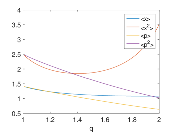
Figure 1: Our four relevant mean values are plotted vs. q.

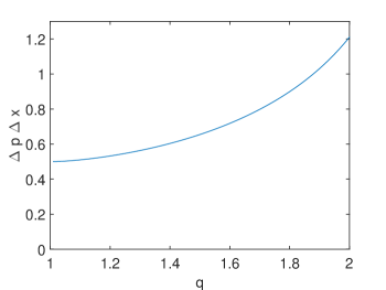
Figure 2: Quantum uncertainties vs. q

Fig. 1 displays the q-dependence of our four relevant q-mean values. With the mean q-values obtained above, we can calculate $(\Delta x)_{q}(\Delta p)_{q}$. The uncertainties are plotted, as a function of $q$, in Fig. 2.

4.5 $\psi_{\alpha q}$ states form an over-complete basis

It is easy to see that there is a one-to-one mapping $|\alpha>\Leftrightarrow|\alpha,q>$, that immediately arises from the well known one-to-one mapping between q-exponentials and ordinary ones. This entails that one can write the unity operator as

$$I=\int\limits_{-\infty}^{\infty}|\alpha,q>A(q,\alpha)<\alpha,q|\;d^{2}\alpha=\frac{1}{\pi}\int\limits_{-\infty}^{\infty}|\alpha><\alpha|\;d^{2}\alpha,$$ (4.27)

with $A(q,\alpha)$ an still unknown constant. Here $\lim_{q\rightarrow 1}A(q,\alpha)=\frac{1}{\pi}$

Thus, for any q, the basis $\{|\alpha,q>\}$ constitute an over complete basis.

5 Quantum uncertainty in the limit $q\rightarrow 1$

We will show now that $\lim_{q\rightarrow 1}(\Delta x)_{q}(\Delta p)_{q}=\Delta x\Delta p=\frac{1}{2}$. This is to the essence in order to ensure that our q-extension of coherent states makes sense. For this endeavor we use the approximation, for $q$ close to one, of the q-exponential. It is easily seen that one has

$$\left[1+i(q-1)z\right]^{\frac{1}{1-q}}=\left[1-\frac{q-1}{2}z^{2}\right]e^{-iz}.$$ (5.1)

As a consequence of (5.1) we obtain

$$\left[1+\frac{q-1}{2}(x^{2}-2\sqrt{2}\alpha x+\alpha^{2}+|\alpha|^{2})\right]^{\frac{1}{1-q}}=$$

$$\left[1+\frac{q-1}{8}(x^{2}-2\sqrt{2}\alpha x+\alpha^{2}+|\alpha|^{2})^{2}\right]e^{-\frac{1}{2}(x^{2}-2\sqrt{2}\alpha x+\alpha^{2}+|\alpha|^{2})}=$$

$$\left(1+\frac{q-1}{2}\frac{\partial^{2}}{\partial\beta^{2}}\right)e^{-\frac{\beta}{2}(x^{2}-2\sqrt{2}\alpha x+\alpha^{2}+|\alpha|^{2})}\left|{}_{\beta=1}\right.$$ (5.2)

The normalized q-coherent state reads, in this approximation,

$$\psi_{\alpha q}(x)=A^{-1}(q,\alpha)\left(1+\frac{q-1}{2}\frac{\partial^{2}}{\partial\beta^{2}}\right)e^{-\frac{\beta}{2}(x^{2}-2\sqrt{2}\alpha x+\alpha^{2}+|\alpha|^{2})}\left|{}_{\beta=1}\right.$$ (5.3)

Of course, $A(q,\alpha)$ needs evaluation. For this purpose we calculate

$$A^{2}(q,\alpha)=\left(1+\frac{q-1}{2}\frac{\partial^{2}}{\partial\beta^{2}}\right)\left(1+\frac{q-1}{2}\frac{\partial^{2}}{\partial\gamma^{2}}\right)\otimes$$

$$\int\limits_{-\infty}^{\infty}e^{-\frac{\beta}{2}(x^{2}-2\sqrt{2}\alpha^{\ast}x+\alpha^{\ast 2}+|\alpha|^{2})}e^{-\frac{\gamma}{2}(x^{2}-2\sqrt{2}\alpha x+\alpha^{2}+|\alpha|^{2})}dx\left|{}_{\beta=\gamma=1}\right.$$ (5.4)

By recourse to the Integral-Table result given in [31] we then find

$$A^{2}(q,\alpha)=\sqrt{\pi}\left(1+\frac{q-1}{2}\frac{\partial^{2}}{\partial\beta^{2}}\right)\left(1+\frac{q-1}{2}\frac{\partial^{2}}{\partial\gamma^{2}}\right)\otimes$$

$$\left[\frac{\sqrt{2}}{\sqrt{\beta+\gamma}}e^{-\frac{\beta}{2}(\alpha^{\ast 2}+|\alpha|^{2})}e^{-\frac{\gamma}{2}(\alpha^{2}+|\alpha|^{2})}e^{\frac{(\beta\alpha^{\ast}+\gamma\alpha)^{2}}{\beta+\gamma}}\right]_{\beta=\gamma=1}.$$ (5.5)

We can thus write

$$A^{2}(q,\alpha)=\sqrt{\pi}+(q-1)f_{1}(\alpha)+(q-1)^{2}f_{2}(\alpha),$$ (5.6)

where $f_{1}$ and $f_{2}$ are non-singular functions of $\alpha$. As a consequence,

$$A(q,\alpha)=\sqrt{\sqrt{\pi}+(q-1)f_{1}(\alpha)+(q-1)^{2}f_{2}(\alpha)},$$ (5.7)

and

$$\lim_{q\rightarrow 1}A(q,\alpha)=\pi^{\frac{1}{4}}.$$ (5.8)

We now can write for $<x^{2}>_{q}$

$$<x^{2}>_{q}=A^{-2}(q,\alpha)\left(1+\frac{q-1}{2}\frac{\partial^{2}}{\partial\beta^{2}}\right)\left(1+\frac{q-1}{2}\frac{\partial^{2}}{\partial\gamma^{2}}\right)\otimes$$

$$\int\limits_{-\infty}^{\infty}e^{-\frac{\beta}{2}(x^{2}-2\sqrt{2}\alpha^{\ast}x+\alpha^{\ast 2}+|\alpha|^{2})}x^{2}e^{-\frac{\gamma}{2}(x^{2}-2\sqrt{2}\alpha x+\alpha^{2}+|\alpha|^{2})}dx\left|{}_{\beta=\gamma=1}\right.$$ (5.9)

Using once more the Integral-Table [31], one has

$$<x^{2}>_{q}=A^{-2}(q,\alpha)\left(1+\frac{q-1}{2}\frac{\partial^{2}}{\partial\beta^{2}}\right)\left(1+\frac{q-1}{2}\frac{\partial^{2}}{\partial\gamma^{2}}\right)\otimes$$

$$\left\{\frac{2^{\frac{3}{2}}}{(\beta+\gamma)^{\frac{3}{2}}}e^{-\frac{\beta}{2}(\alpha^{\ast 2}+|\alpha|^{2})}e^{-\frac{\gamma}{2}(\alpha^{2}+|\alpha|^{2})}e^{\frac{(\beta\alpha^{\ast}+\gamma\alpha)^{2}}{\beta+\gamma}}(2i)^{-2}\sqrt{\pi}H_{2}\left[\frac{i(\beta\alpha^{\ast}+\gamma\alpha)}{\sqrt{\beta+\gamma}}\right]\right\}.$$ (5.10)

As a consequence,

$$<x^{2}>_{q}=A^{-2}(q,\alpha)\left\{\sqrt{\pi}\left[\frac{(\alpha+\alpha^{\ast})^{2}}{2}+\frac{1}{2}\right]+(q-1)g_{1}(\alpha)+(q-1)^{2}g_{2}(\alpha)\right\},$$ (5.11)

where $g_{1}$ and $g_{2}$ are non-singular functions of $\alpha$. Thus (See Appendix C),

$$\lim_{q\rightarrow 1}<x^{2}>_{q}=\frac{1}{2}+\frac{(\alpha+\alpha^{\ast})^{2}}{2}=<x^{2}>.$$ (5.12)

Proceeding now in similar fashion for $<x>_{q}$ we obtain

$$<x>_{q}=A^{-2}(q,\alpha)\left(1+\frac{q-1}{2}\frac{\partial^{2}}{\partial\beta^{2}}\right)\left(1+\frac{q-1}{2}\frac{\partial^{2}}{\partial\gamma^{2}}\right)\otimes$$

$$\int\limits_{-\infty}^{\infty}e^{-\frac{\beta}{2}(x^{2}-2\sqrt{2}\alpha^{\ast}x+\alpha^{\ast 2}+|\alpha|^{2})}xe^{-\frac{\gamma}{2}(x^{2}-2\sqrt{2}\alpha x+\alpha^{2}+|\alpha|^{2})}dx\left|{}_{\beta=\gamma=1}\right.$$ (5.13)

According to the Integral-Table result [31],

$$<x>_{q}=A^{-2}(q,\alpha)\left(1+\frac{q-1}{2}\frac{\partial^{2}}{\partial\beta^{2}}\right)\left(1+\frac{q-1}{2}\frac{\partial^{2}}{\partial\gamma^{2}}\right)\otimes$$

$$\left\{\frac{2}{\beta+\gamma)}e^{-\frac{\beta}{2}(\alpha^{\ast 2}+|\alpha|^{2})}e^{-\frac{\gamma}{2}(\alpha^{2}+|\alpha|^{2})}e^{\frac{(\beta\alpha^{\ast}+\gamma\alpha)^{2}}{\beta+\gamma}}(2i)^{-1}\sqrt{\pi}H_{1}\left[\frac{i(\beta\alpha^{\ast}+\gamma\alpha)}{\sqrt{\beta+\gamma}}\right]\right\},$$ (5.14)

or

$$<x>_{q}=A^{-2}(q,\alpha)\left\{\sqrt{\pi}\left[\frac{\alpha+\alpha^{\ast}}{\sqrt{2}}\right]+(q-1)h_{1}(\alpha)+(q-1)^{2}h_{2}(\alpha)\right\},$$ (5.15)

where $h_{1}$ and $h_{2}$ are again non-singular functions of $\alpha$. Accordingly (see Appendix C),

$$\lim_{q\rightarrow 1}<x>_{q}=\frac{\alpha+\alpha^{\ast}}{\sqrt{2}}=<x>.$$ (5.16)

For $<p^{2}>_{q}$ we have instead

$$<p^{2}>_{q}=-A^{-2}(q,\alpha)\left(1+\frac{q-1}{2}\frac{\partial^{2}}{\partial\beta^{2}}\right)\left(1+\frac{q-1}{2}\frac{\partial^{2}}{\partial\gamma^{2}}\right)\otimes$$

$$\int\limits_{-\infty}^{\infty}e^{-\frac{\beta}{2}(x^{2}-2\sqrt{2}\alpha^{\ast}x+\alpha^{\ast 2}+|\alpha|^{2})}\frac{\partial^{2}}{\partial x^{2}}e^{-\frac{\gamma}{2}(x^{2}-2\sqrt{2}\alpha x+\alpha^{2}+|\alpha|^{2})}dx\left|{}_{\beta=\gamma=1}\right.$$ (5.17)

or

$$<p^{2}>_{q}=A^{-2}(q,\alpha)\left(1+\frac{q-1}{2}\frac{\partial^{2}}{\partial\beta^{2}}\right)\left(1+\frac{q-1}{2}\frac{\partial^{2}}{\partial\gamma^{2}}\right)\otimes$$

$$\int\limits_{-\infty}^{\infty}e^{-\frac{\beta}{2}(x^{2}-2\sqrt{2}\alpha^{\ast}x+\alpha^{\ast 2}+|\alpha|^{2})}[\gamma^{2}(x-\sqrt{2}\alpha)^{2}-\gamma]e^{-\frac{\gamma}{2}(x^{2}-2\sqrt{2}\alpha x+\alpha^{2}+|\alpha|^{2})}dx\left|{}_{\beta=\gamma=1}\right.$$ (5.18)

As in previous cases, according to Integral-Table result [31] we have

$$<p^{2}>_{q}=A^{-2}(q,\alpha)\left\{\sqrt{\pi}\left[\frac{1}{2}-\frac{(\alpha-\alpha^{\ast})^{2}}{2}\right]+(q-1)k_{1}(\alpha)+(q-1)^{2}k_{2}(\alpha)\right\}.$$ (5.19)

Here $k_{1}$ and $k_{2}$ are non-singular functions as well. Therefore (see Appendix C),

$$\lim_{q\rightarrow 1}<p^{2}>_{q}=\frac{1}{2}-\frac{(\alpha-\alpha^{\ast})^{2}}{2}=<p^{2}>.$$ (5.20)

In analogy with the above case we now also have

$$<p>_{q}=-iA^{-2}(q,\alpha)\left(1+\frac{q-1}{2}\frac{\partial^{2}}{\partial\beta^{2}}\right)\left(1+\frac{q-1}{2}\frac{\partial^{2}}{\partial\gamma^{2}}\right)\otimes$$

$$\int\limits_{-\infty}^{\infty}e^{-\frac{\beta}{2}(x^{2}-2\sqrt{2}\alpha^{\ast}x+\alpha^{\ast 2}+|\alpha|^{2})}\frac{\partial}{\partial x}e^{-\frac{\gamma}{2}(x^{2}-2\sqrt{2}\alpha x+\alpha^{2}+|\alpha|^{2})}dx\left|{}_{\beta=\gamma=1}\right.$$ (5.21)

and, after employing again the Integral-Table result [31],

$$<p>_{q}=-iA^{-2}(q,\alpha)\left\{\sqrt{\pi}\left[\frac{\alpha-\alpha^{\ast}}{\sqrt{2}}\right]+(q-1)l_{1}(\alpha)+(q-1)^{2}l_{2}(\alpha)\right\},$$ (5.22)

where $l_{1}$ and $l_{2}$ are non-singular functions of $\alpha$. Thus (see Appendix C),

$$\lim_{q\rightarrow 1}<p>_{q}=\frac{\alpha-\alpha^{\ast}}{i\sqrt{2}}=<p>.$$ (5.23)

From (5.12), (5.16), (5.20), and (5.23), we obtain

$$\lim_{q\rightarrow 1}(\Delta x)_{q}(\Delta p)_{q}=\Delta x\Delta p=\frac{1}{2}.$$ (5.24)

For the q-distribution, with q close to 1, and using

$$|q,\alpha>=A^{-1}(q,\alpha)\left(1+\frac{q-1}{2}\frac{\partial^{2}}{\partial\beta^{2}}\right)\int\limits_{-\infty}^{\infty}e^{-\frac{\beta}{2}(x^{2}-2\sqrt{2}\alpha^{\ast}x+\alpha^{\ast 2}+|\alpha|^{2})}|x>dx\left|{}_{\beta=1}\right.$$ (5.25)

we have

$$<k|q,\alpha>=\frac{A^{-1}(q,\alpha)}{\sqrt{2\pi}}\left(1+\frac{q-1}{2}\frac{\partial^{2}}{\partial\beta^{2}}\right)\otimes$$

$$\int\limits_{-\infty}^{\infty}e^{-ikx}e^{-\frac{\beta}{2}(x^{2}-2\sqrt{2}\alpha x+\alpha^{2}+|\alpha|^{2})}dx\left|{}_{\beta=1}\right.$$ (5.26)

Again, from the Integral-Table result [31], we can write

$$<k|q,\alpha>=A^{-1}(q,\alpha)\left[e^{-\frac{1}{2}(k^{2}+2\sqrt{2}i\alpha k-\alpha^{2}+|\alpha|^{2})}+(q-1)f(\alpha,k)\right],$$ (5.27)

where $f$ is non-singular. Using the results given there we have

$$\lim_{q\rightarrow 1}<k|q,\alpha>=\pi^{-\frac{1}{4}}e^{-\frac{1}{2}(k^{2}+2\sqrt{2}i\alpha k-\alpha^{2}+|\alpha|^{2})}=<k|\alpha>,$$ (5.28)

and, as a consequence,

$$\lim_{q\rightarrow 1}|<k|q,\alpha>|^{2}=|<k|\alpha>|^{2}=\pi^{-\frac{1}{2}}e^{-(k-p)^{2}},$$ (5.29)

a nice result indeed!

6 Conclusions

We have introduced and studied in this work special q-states that one might denominate Tsallis’ pseudo-coherent ones (that have nothing to do with the so-called q-coherent states of Quesne, Eremin-Meldianov, and others [22].) Also, we obtained some interesting preliminary results. In particular, we have exhibited the q-dependence of the quantum uncertainty, that is minimal for $q=1$. We emphasize that we have gotten the first overcomplete basis of Tsallis literature. This should be an interesting addition to such body of work. Summing up:

• We determined the most important relationships governing the new Tsallis’ pseudo-coherent states.

• In particular, let us reiterate, we find that, in the limit $q\rightarrow 1$, minimal uncertainty is attained (for $q=1$), which constitutes a fundamental result.

• We saw that the Tsallis’ pseudo-coherent states constitute an over complete basis for any $q$.

Appendix A: Proof of Eq.(2.9)

It is very well known the annihilation operator for the one-dimensional harmonic oscillator is given by

$$\hat{a}=\frac{\hat{x}+i\hat{p}}{\sqrt{2}}$$ (A.1)

In the x-representation of Quantum Mechanics this operator is expressed via

$$\hat{a}(x)=\frac{1}{\sqrt{2}}\left(x+\frac{d}{dx}\right)$$ (A.2)

Thus, a coherent state is defined as the eigenfunction

$$\hat{a}(x)\psi_{\alpha}(x)=\frac{1}{\sqrt{2}}\left(x\psi_{\alpha}(x)+\frac{d\psi_{\alpha}(x)}{dx}\right)=\alpha\psi_{\alpha}(x),$$ (A.3)

or, equivalently,

$$\frac{d\psi_{\alpha}(x)}{dx}=(\sqrt{2}\alpha-x)\psi_{\alpha}(x).$$ (A.4)

The solution of (A.4) is

$$\psi_{\alpha}(x)=Ce^{-\frac{x^{2}}{2}}e^{\sqrt{2}\alpha x}.$$ (A.5)

The constant $C$ can be evaluated using the normalization condition

$$\int\limits_{-\infty}^{\infty}|\psi_{\alpha}(x)|^{2}dx=|C|^{2}\int\limits_{-\infty}^{\infty}e^{-x^{2}}e^{\sqrt{2}(\alpha+{\alpha}^{\ast})x}dx=1.$$ (A.6)

Accordingly,

$$\int\limits_{-\infty}^{\infty}|\psi_{\alpha}(x)|^{2}dx=|C|^{2}e^{\frac{(\alpha+{\alpha}^{\ast})^{2}}{2}}\int\limits_{-\infty}^{\infty}e^{-\left(x-\frac{\alpha+{\alpha}^{\ast}}{\sqrt{2}}\right)^{2}}dx=1.$$ (A.7)

By recourse to the result given in the Table [31] we now obtain

$$\int\limits_{-\infty}^{\infty}e^{-\left(x-\frac{\alpha+{\alpha}^{\ast}}{\sqrt{2}}\right)^{2}}dx=\sqrt{\pi}.$$ (A.8)

As a consequence,

$$C=\pi^{-\frac{1}{4}}e^{-\frac{(\alpha+{\alpha}^{\ast})^{2}}{4}}.$$ (A.9)

Thus, we have for $\psi_{\alpha}(x)$ the expression

$$\psi_{\alpha}(x)=\pi^{-\frac{1}{4}}e^{-\frac{(\alpha+{\alpha}^{\ast})^{2}}{4}}e^{-\frac{x^{2}}{2}}e^{\sqrt{2}\alpha x},$$ (A.10)

or, equivalently,

$$\psi_{\alpha}(x)=e^{i\alpha_{R}\alpha_{I}}\pi^{-\frac{1}{4}}e^{-\frac{\alpha^{2}}{2}}e^{-\frac{|\alpha|^{2}}{2}}e^{-\frac{x^{2}}{2}}e^{\sqrt{2}\alpha x},$$ (A.11)

where $\alpha=\alpha_{R}+i\alpha_{I}$. As $e^{i\alpha_{R}\alpha_{I}}$ is an imaginary phase, it can be eliminated from (A.11) to finally obtain

$$\psi_{\alpha}(x)=\pi^{-\frac{1}{4}}e^{-\frac{\alpha^{2}}{2}}e^{-\frac{|\alpha|^{2}}{2}}e^{-\frac{x^{2}}{2}}e^{\sqrt{2}\alpha x}.$$ (A.12)

Appendix B: Lauricella functions

Lauricella functions $F$ can be regarded as generalizations to several variables of the Gauss hypergeometric functions. They were investigated at the end of the 19ts century by Giuseppe Lauricella (1867–1913), an Italian mathematician mostly known by his contribution to elasticity theory. The fourth Lauricella function of four variables is given by [32]

$$F_{D}(a;b_{1},b_{2},b_{3},b_{4};c;x_{1},x_{2},x_{3},x_{4})=$$

$$\sum\limits_{m_{1}=0}^{\infty}\sum\limits_{m_{2}=0}^{\infty}\sum\limits_{m_{3}=0}^{\infty}\sum\limits_{m_{4}=0}^{\infty}\frac{(a)_{m_{1}+m_{2}+m_{3}+m_{4}}(b_{1})_{m_{1}}(b_{2})_{m_{2}}(b_{3})_{m_{3}}(b_{4})_{m_{4}}}{(c)_{m_{1}+m_{2}+m_{3}+m_{4}}}\otimes$$

$$\frac{x_{1}^{m_{1}}x_{2}^{m_{2}}x_{3}^{m_{3}}x_{4}^{m_{4}}}{m_{1}!m_{2}!m_{3}!m_{4}!}.$$ (B.1)

This function satisfies [32]

$$\int\limits_{0}^{1}u^{a-1}(1-u)^{c-a-1}(1-ux_{1})^{-b_{1}}(1-ux_{2})^{-b_{2}}(1-ux_{3})^{-b_{3}}(1-ux_{4})^{-b_{4}}du$$

$$=\frac{\Gamma(a)\Gamma(c-a)}{\Gamma(c)}F_{D}(a;b_{1},b_{2},b_{3},b_{4};c;x_{1},x_{2},x_{3},x_{4}).$$ (B.2)

After two variables’ changes we can deduce, from (B.2), the relation

$$\int\limits_{0}^{\infty}u^{c-a-1}(1-u)^{b_{1}+b_{2}+b_{3}+b_{4}-c}(u_{1}+z_{1})^{-b_{1}}(u_{2}+z_{2})^{-b_{2}}(u_{3}+z_{3})^{-b_{3}}(u_{4}+z_{4})^{-b_{4}}du$$

$$=\frac{\Gamma(a)\Gamma(c-a)}{\Gamma(c)}F_{D}(a;b_{1},b_{2},b_{3},b_{4};c;1-z_{1},1-z_{2},1-z_{3},1-z_{4}).$$ (B.3)

Appendix C: Reviewing uncertainty relations for coherent states

For the sake of completeness, we give here some well known results that are needed in determining uncertainties. For an ordinary coherent state $|\alpha>$ we have:

$$<x^{2}>=\pi^{-\frac{1}{2}}\int\limits_{-\infty}^{\infty}e^{-\frac{1}{2}(x^{2}-2\sqrt{2}\alpha^{\ast}x+\alpha^{\ast 2}+|\alpha|^{2})}x^{2}e^{-\frac{1}{2}(x^{2}-2\sqrt{2}\alpha x+\alpha^{2}+|\alpha|^{2})}dx$$ (C.1)

With the use of the Integral-Table result [31] we find

$$<x^{2}>=(2i)^{-2}H_{2}\left[\frac{i(\alpha^{\ast}+\alpha)}{\sqrt{2}}\right]$$ (C.2)

and then

$$<x^{2}>=\frac{1}{2}+\frac{(\alpha+\alpha^{\ast})^{2}}{2}$$ (C.3)

For $<x>$ the situation is quite similar

$$<x>=\pi^{-\frac{1}{2}}\int\limits_{-\infty}^{\infty}e^{-\frac{1}{2}(x^{2}-2\sqrt{2}\alpha^{\ast}x+\alpha^{\ast 2}+|\alpha|^{2})}xe^{-\frac{1}{2}(x^{2}-2\sqrt{2}\alpha x+\alpha^{2}+|\alpha|^{2})}dx$$ (C.4)

Using the Integral-Table result [31] again we obtain

$$<x>=(2i)^{-1}H_{1}\left[\frac{i(\alpha^{\ast}+\alpha)}{\sqrt{2}}\right]$$ (C.5)

and thus

$$<x>=\frac{\alpha+\alpha^{\ast}}{\sqrt{2}}$$ (C.6)

For $<p>$, the integral is somewhat more complicated

$$<p^{2}>=-\pi^{-\frac{1}{2}}\int\limits_{-\infty}^{\infty}e^{-\frac{1}{2}(x^{2}-2\sqrt{2}\alpha^{\ast}x+\alpha^{\ast 2}+|\alpha|^{2})}\frac{\partial^{2}}{\partial x^{2}}e^{-\frac{1}{2}(x^{2}-2\sqrt{2}\alpha x+\alpha^{2}+|\alpha|^{2})}dx$$ (C.7)

or:

$$<p^{2}>=\pi^{-\frac{1}{2}}\int\limits_{-\infty}^{\infty}e^{-\frac{1}{2}(x^{2}-2\sqrt{2}\alpha^{\ast}x+\alpha^{\ast 2}+|\alpha|^{2})}[1-(x-\sqrt{2}\alpha)^{2}]e^{-\frac{1}{2}(x^{2}-2\sqrt{2}\alpha x+\alpha^{2}+|\alpha|^{2})}dx$$ (C.8)

Now, by recourse to the Integral-Table result [31] we obtain

$$<p^{2}>=1-2\alpha^{2}-i\sqrt{2}\alpha H_{1}\left[\frac{i(\alpha^{\ast}+\alpha)}{\sqrt{2}}\right]+\frac{1}{4}H_{2}\left[\frac{i(\alpha^{\ast}+\alpha)}{\sqrt{2}}\right]$$ (C.9)

or

$$<p^{2}>=\frac{1}{2}-\frac{(\alpha-\alpha^{\ast})^{2}}{2}$$ (C.10)

For dealing with $<p>$ one starts with

$$<p>=-i\pi^{-\frac{1}{2}}\int\limits_{-\infty}^{\infty}e^{-\frac{1}{2}(x^{2}-2\sqrt{2}\alpha^{\ast}x+\alpha^{\ast 2}+|\alpha|^{2})}\frac{\partial}{\partial x}e^{-\frac{1}{2}(x^{2}-2\sqrt{2}\alpha x+\alpha^{2}+|\alpha|^{2})}dx$$ (C.11)

or

$$<p>=i\pi^{-\frac{1}{2}}\int\limits_{-\infty}^{\infty}e^{-\frac{1}{2}(x^{2}-2\sqrt{2}\alpha^{\ast}x+\alpha^{\ast 2}+|\alpha|^{2})}(x-\sqrt{2}\alpha)e^{-\frac{1}{2}(x^{2}-2\sqrt{2}\alpha x+\alpha^{2}+|\alpha|^{2})}dx$$ (C.12)

and, finally,

$$<p>=\frac{\alpha-\alpha^{\ast}}{i\sqrt{2}}$$ (C.13)

Accordingly, the well-known uncertainty relation for a coherent state becomes

$$\Delta x\Delta p=\frac{1}{2},$$ (C.14)

i.e., minimal uncertainty, the main feature of coherent state.

References

- [1] C. Tsallis, J. of Stat. Phys., 52 (1988) 479.
- [2] C. Tsallis, Introduction to Nonextensive Statistical Mechanics: Approaching a Complex World (Springer, NY, 2009).
- [3] A. Adare et al., Phys. Rev. D 83 (2011) 052004.
- [4] G. Wilk, Z. Wlodarczyk, Physica A 305 (2002) 227.
- [5] R. M. Pickup, R. Cywinski, C. Pappas, B. Farago, and P. Fouquet, Phys. Rev. Lett. 102 (2009) 097202.
- [6] E. Lutz and F. Renzoni, Nature Physics 9 (2013) 615.
- [7] R. G. DeVoe, Phys. Rev. Lett. 102 (2009) 063001.
- [8] Z. Huang, G. Su, A. El Kaabouchi, Q. A. Wang, and J. Chen, J. Stat. Mech. L05001 (2010).
- [9] J. Prehl, C. Essex, and K. H. Hoffman, Entropy 14 (2012) 701.
- [10] B. Liu and J. Goree, Phys. Rev. Lett. 100 (2018) 055003.
- [11] O. Afsar and U. Tirnakli, EPL 101 (2013) 20003.
- [12] U. Tirnakli, C. Tsallis, and C. Beck, Phys. Rev. E 79 (2009) 056209.
- [13] G. Ruiz, T. Bountis, and C. Tsallis, Int. J. Bifurcation Chaos 22 (2012) 1250208.
- [14] C. Beck and S. Miah, Phys. Rev. E 87 (2013) 031002.
- [15] H. J. Carmichael:”Statistical Methods in Quantum Optics: Master Equations and Fokker-Planck Equations. Texts and Monographs in Physics”. Springer (1998).
- [16] G. Wilk, Z. Wlodarczyk, Phys. Rev. Lett. 84 (2000) 2770.
- [17] J. Rozynek, G. Wilk, J. of Physics G 36 (2009) 125108.
- [18] C. M. Gell-Mann and C. Tsallis, Nonextensive Entropy-Interdisciplinary Applications (Oxford University Press, New York, 2004).
- [19] S. Abe, Astrophys. Space Sci. 305 (2006) 241.
- [20] S. Picoli, R. S. Mendes, L. C. Malacarne, and R. P. B. Santos, Braz. J. Phys. 39 (2009) 468.
- [21] F.D. Nobre, M.A. Rego-Monteiro, C. Tsallis, Phys. Rev. Lett. 106 (2011) 140601.
- [22] C. Quesne, ArXiv: quant-ph/0206188 (2002); V.V Eremin, A.A. Meldianov, ArXiv: quant-ph/ 0810.1967 (2008).
- [23] R. J. Glauber, Phys. Rev. Lett. 10, 84 (1963).
- [24] R. J. Glauber, Phys. Rev. 130, 2529 (1963).
- [25] R. J. Glauber, Phys. Rev. 131, 493 (1963).
- [26] R. J. Glauber, Quantum Optics and Electronics, ed. C. deWitt, A. Blandin, and C. Cohen-Tannoudji (Gordon and Breach, New York, 1965).
- [27] I. S. Gradshteyn and I. M. Ryzhik: ”Table of Integrals, Series and Products”, 7.374,6, p.837. Academic Press (1965).
- [28] I. S. Gradshteyn and I. M. Ryzhik: ”Table of Integrals, Series and Products”, 3.462,1, p.337. Academic Press (1965).
- [29] H. J. Carmichael:” Statistical Methods in Quantum Optics I. Master Equations and Fokker-Planck Equations”. Springer-Verlag Berlin Heidelberg (1999).
- [30] I. S. Gradshteyn and I. M. Ryzhik: ”Table of Integrals, Series and Products”, 3.384,7 and 8, p.320. Academic Press (1965).
- [31] I. S. Gradshteyn and I. M. Ryzhik: ”Table of Integrals, Series and Products”, 3.462,4, p.338. Academic Press (1965).
- [32] A. M. Mathai, Hans J. Haubold: ”Special Functions for Applied Scientists”- Springer (2008).