Reflection and Refraction of the Laser Light Pulse at the Vacuum–Medium Interface

Abstract

By generalizing the well known results for reflection and refraction of plane waves at the vacuum–medium interface to Gaussian light beams, we obtain analytic formulas for reflection and refraction of the TM and TE laser light pulses. This enables us to give a possible explanation why no reflection was observed in light pulse photographs in some vicinity of the air–resin interface, given in L. Gao, J. Liang, C. Li, and L. V. Wang, Nature 516, 74 (2014). We suggest how to modify the experimental setup so as to observe the reflected pulse.

I Introduction

In an impressive paper Gao et al. (2014a) describing ultrafast photography ($10^{11}$ frames per second), among examples given there was a laser light pulse photograph in some vicinity of the vacuum–resin interface, see Fig. 3(b) in Gao et al. (2014a). The transmitted pulse could be seen there, but no reflected one was observed. Here we try to explain why there was no reflection, and how to modify the experimental setup to observe it.

In Sec. II we show that the Gaussian beams for which the transverse dimensions are constant along the beam, behave in full analogy to plane waves, and we derive formulas pertaining to their reflection and refraction at the plane vacuum–medium interface.

Section III deals with reflection and refraction of laser pulses, and Sec. IV specifies these results to the pulses used in Gao et al. (2014a) and contains the final conclusions.

We assume that in our laboratory Cartesian coordinate system ($x,y,z$), with a medium at $y<0$ and vacuum at $y>0$, we can fulfil the boundary conditions at the interface, $y=0$, by a superposition of three beams propagating in the $x,y$ plane: the incident (i), reflected (r) and refracted (or transmitted, t) Gaussian beam. In the paraxial approximation, we can describe any such steady state TM beam as Goldsmith (1998); Scheck (2012) (Gaussian units)

$$H_{z_{\text{i,r,t}}} = C_{\text{i,r,t}}\exp\biggl{(}-\frac{x^{2}_{\text{i,r,t}}}{w_{x_{\text{i,r,t}}}^{2}}-\frac{z^{2}}{w_{z}^{2}}\biggr{)}$$ (1a)

$$\times\exp\bigl{\{}i\bigl{[}(ky)_{\text{i,r,t}}-\omega t\bigr{]}\bigr{\}},$$

$$E_{x_{\text{i,r,t}}} = -Z_{\text{i,r,t}}H_{z_{\text{i,r,t}}},\qquad k_{\text{i,r,t}}=\omega\,n_{\text{i,r,t}}/c,$$ (1b)

where $C_{\text{i}}=1$, $C_{\text{r}}=R_{\text{TM}}$ is the reflection coefficient, $C_{\text{t}}=T_{\text{TM}}$ is the transmission coefficient, $y_{\text{i,r,t}}$ are Cartesian coordinates along each beam, $x_{\text{i,r,t}}$ are similar coordinates for transverse directions, $\omega$ is the angular frequency, $c$ is the speed of light in vacuum, $k_{\text{i,r,t}}$ are the wave numbers, $n_{\text{i,r}}=1$ and $n_{\text{t}}=n\equiv\sqrt{\epsilon\mu}$ are the refraction indexes of vacuum and medium, $Z_{\text{i,r}}=1$ and $Z_{\text{t}}=\sqrt{\mu/\epsilon}$ are similar field impedances, and the positive constants $\epsilon$ and $\mu$ characterize the medium.

Note that for each beam, the radii $w_{x}$ and $w_{z}$ are constant here ($y$ independent), which requires $y$ to be small as compared to the Rayleigh ranges $\hat{y}_{x}$ and $\hat{y}_{z}$:

$$(y/\hat{y}_{x,z})^{2}\ll 1,\qquad\hat{y}_{x,z}=\pi w_{x,z}^{2}/\lambda,$$ (2)

where $\lambda=(c/n)2\pi/\omega$ is the wavelength.

Note that by TM (or TE) polarization we mean orthogonality of the H (or E) vector with respect to the plane of incidence ($x$, $y$ in our case).

II Boundary conditions

In the limit $w_{x}\to\infty$ and $w_{z}\to\infty$ in (1), we obtain the plane waves: $H_{z}=C\exp\bigl{[}i(ky-\omega t)\bigr{]}$. Therefore in this limit, the continuity of the tangential components of E and H for the incident plus reflected beam versus the transmitted one at the interface ($y=0$) implies the Snell law

$$\varphi_{\text{r}}=\varphi_{\text{i}},\qquad n\sin\varphi_{\text{t}}=\sin\varphi_{\text{i}},$$ (3)

and the Fresnel formulas Scheck (2012); Jackson (1999) $\bigl{(}\nu=n\cos\varphi_{\text{t}}\bigr{)}$

$$R_{\text{TM}} =\frac{\epsilon\cos\varphi_{\text{i}}-\nu}{\epsilon\cos\varphi_{\text{i}}+\nu}, T_{\text{TM}} =1+R_{\text{TM}},$$ (4a)

$$R_{\text{TE}} =\frac{\mu\cos\varphi_{\text{i}}-\nu}{\mu\cos\varphi_{\text{i}}+\nu}, T_{\text{TE}} =1+R_{\text{TE}},$$ (4b)

where $\varphi_{\text{i}}$, $\varphi_{\text{r}}$ and $\varphi_{\text{t}}$ are the angles of incidence, reflection and refraction.

For finite radii $w_{x_{\text{i,r,t}}}$ and $w_{z}=w_{z_{\text{i,r,t}}}$, we have to take into account linear relations defining $x_{\text{i,r,t}}$ and $y_{\text{i,r,t}}$ as functions of the laboratory $x$ and $y$ ($z_{\text{i,r,t}}=-z$):

$$x_{\text{i,r,t}}=(x,y)\cdot\hat{\mathbf{x}}_{\text{i,r,t}},\qquad y_{\text{i,r,t}}=(x,y)\cdot\hat{\mathbf{y}}_{\text{i,r,t}},$$ (5)

where hats denote unit vectors for local coordinate axes of each beam,

$$\hat{\mathbf{x}}_{\text{i,r}}=(\pm\cos\varphi_{\text{i}},\sin\varphi_{\text{i}}),\qquad\hat{\mathbf{x}}_{\text{t}}=(\cos\varphi_{\text{t}},\sin\varphi_{\text{t}}),$$ (6)

$$\hat{\mathbf{y}}_{\text{i,r}}=(\sin\varphi_{\text{i}},\mp\cos\varphi_{\text{i}}),\qquad\hat{\mathbf{y}}_{\text{t}}=(\sin\varphi_{\text{t}},-\cos\varphi_{\text{t}}).$$ (7)

At the boundary, $y=0$, equations (5) lead to

$$\frac{x^{2}_{\text{i,r}}}{w_{x_{\text{i,r}}}^{2}}=x^{2}\frac{\cos^{2}\varphi_{\text{i}}}{w_{x_{\text{i,r}}}^{2}},\qquad\frac{x^{2}_{\text{t}}}{w_{x_{\text{t}}}^{2}}=x^{2}\frac{\cos^{2}\varphi_{\text{t}}}{w_{x_{\text{t}}}^{2}}.$$ (8)

Thus if $x=z=0$, Eq. (1) is the same as that for plane waves, and the boundary conditions are satisfied. They will be satisfied also for nonzero $x$ and $z$, if the RHSs of (8) are the same, i.e., if

$$w_{x_{\text{r}}}=w_{x_{\text{i}}},\qquad w_{x_{\text{t}}}=w_{x_{\text{i}}}\frac{\cos\varphi_{\text{t}}}{\cos\varphi_{\text{i}}}>w_{x_{\text{i}}}.$$ (9)

For the TE Gaussian beam one has to replace $\text{TM}\to\text{TE}$, $H_{z_{\text{i,r,t}}}\to E_{z_{\text{i,r,t}}}$, and $H_{x_{\text{i,r,t}}}=E_{z_{\text{i,r,t}}}/Z_{\text{i,r,t}}$.

III Specification to laser pulses

If the incident laser beam is not monochromatic, but has a spectrum function $F(\omega)$, we have to include all harmonics, and the time behavior of all beams will be given by the integral (Inverse Fourier Transform)

$$\int_{-\infty}^{\infty}F(\omega)\exp(i\omega\bar{t})\,d\,\omega\qquad\text{at}\qquad\bar{t}=\frac{y_{\text{i,r,t}}}{c/n_{\text{i,r,t}}}-t.$$ (10)

For a Gaussian spectrum function

$$F(\omega)=\exp\{-[(\omega-\omega_{0})/b]^{2}\},$$ (11)

centered about $\omega=\omega_{0}$, the Gaussian wave packets will be obtained. In that case, for a conveniently normalized TM laser beam, we end up with (neglecting the common factor $b\sqrt{\pi}$):

$$H_{z}(y>0) = \exp\biggl{[}-\frac{x_{\text{i}}^{2}}{w_{x_{\text{i}}}^{2}}-\frac{(y_{\text{i}}-ct)^{2}}{w_{y_{\text{i}}}^{2}}-\frac{z^{2}}{w_{z}^{2}}+ik_{0}(y_{\text{i}}-ct)\biggr{]}+R_{\text{TM}}\exp\biggl{[}-\frac{x_{\text{r}}^{2}}{w_{x_{\text{i}}}^{2}}-\frac{(y_{\text{r}}-ct)^{2}}{w_{y_{\text{r}}}^{2}}-\frac{z^{2}}{w_{z}^{2}}+ik_{0}(y_{\text{r}}-ct)\biggr{]},\ \$$ (12)

$$H_{z}(y\leq 0) = (1+R_{\text{TM}})\exp\biggl{[}-\frac{x_{\text{t}}^{2}}{w_{x_{\text{t}}}^{2}}-\frac{(y_{\text{t}}-ct/n)^{2}}{w_{y_{\text{t}}}^{2}}-\frac{z^{2}}{w_{z}^{2}}+ik_{0}n(y_{\text{t}}-ct/n)\biggr{]},$$ (13)

where

$$w_{y_{\text{i}}}=2c/b,\qquad w_{y_{\text{r}}}=w_{y_{\text{i}}},\qquad w_{y_{\text{t}}}=w_{y_{\text{i}}}/n,$$ (14)

are the the light pulse radii along each beam, while $k_{0}=2\pi/\lambda_{0}$, $\lambda_{0}=cT_{0}$ and $T_{0}=2\pi/\omega_{0}$ are the vacuum wavenumber, wavelength and period for the beam carrier, $\omega=\omega_{0}$. See also (5)–(7) and (9) for remaining definitions, in which $\varphi_{\text{t}}=\arcsin[(\sin\varphi_{\text{i}})/n]$.

Replacing $H_{z}\to E_{z}$ and $R_{\text{TM}}\to R_{\text{TE}}$ in (12) and (13), we obtain the TE beam fields.

The real parts of the complex coordinates $H_{z}$ and $E_{z}$ defined above give us the $z$ coordinates of the real physical fields.

From now on, it will be convenient to work with dimensionless variables, by measuring time and space dimensions in the units of $T_{0}$ and $\lambda_{0}$, see Figs. 1–4. This implies $c=1$ and $k_{0}=2\pi$ in (12) and (13).

At $t=0$, for each of the pulses in (12) and (13), the real part is a product of a strongly oscillating function of $y_{\text{i,r,t}}$ [$\cos(2\pi y_{\text{i}})$, $\cos(2\pi y_{\text{r}})$, and $\cos(2\pi ny_{\text{t}})$, with wavelengths $\lambda_{\text{i}}=\lambda_{\text{r}}=1$, $\lambda_{\text{t}}=1/n$], and the envelope which is a Gaussian proportional to

$$\exp\bigl{[}-(\text{space coordinate}/\text{pulse radius})^{2}\bigr{]}.$$ (15)

During time evolution starting at some $t=t_{\text{in}}<0$, the incident and reflected pulses move along the $y_{\text{i}}$ and $y_{\text{r}}$ axes with unit velocities, and the refracted pulse along the $y_{\text{t}}$ axis with the velocity $1/n$.

Notice that there is a common factor $\exp\bigl{(}-z^{2}/w_{z}^{2}\bigr{)}$ in (12) and (13). Its square will appear as a common factor in formulas defining energy densities (time averaged over fast oscillations with $\omega=2\omega_{0}$), proportional to $\mu H_{z}H_{z}^{*}$ and $\epsilon E_{z}E_{z}^{*}$. Integrating these formulas $dz$ from $-\infty$ to $\infty$ we obtain (time averaged) surface energy densities, $\mathcal{E}_{\text{TM}}(x,y,t)$ and $\mathcal{E}_{\text{TE}}(x,y,t)$. Again neglecting the common factor ($w_{z}\sqrt{\pi/2}$), we end up with

$$\mathcal{E}_{\text{TM}}(x,y>0,t) = \exp\biggl{[}-\Bigl{(}\frac{x_{\text{i}}}{w_{x_{\text{i}}}/\sqrt{2}}\Bigr{)}^{2}-\Bigl{(}\frac{y_{\text{i}}-t}{w_{y_{\text{i}}}/\sqrt{2}}\Bigr{)}^{2}\biggr{]}+R_{\text{TM}}^{2}\exp\biggl{[}-\Bigl{(}\frac{x_{\text{r}}}{w_{x_{\text{i}}}/\sqrt{2}}\Bigr{)}^{2}-\Bigl{(}\frac{y_{\text{r}}-t}{w_{y_{\text{i}}}/\sqrt{2}}\Bigr{)}^{2}\biggr{]}$$ (16)

$$+2R_{\text{TM}}\exp\Biggl{[}-\frac{x_{\text{i}}^{2}+x_{\text{r}}^{2}}{w_{x_{\text{i}}}^{2}}-\frac{(y_{\text{i}}-t)^{2}+(y_{\text{r}}-t)^{2}}{w_{y_{\text{i}}}^{2}}\Biggr{]}\cos\bigl{(}4\pi y\cos\varphi_{\text{i}}\bigr{)},$$

$$\mathcal{E}_{\text{TM}}(x,y\leq 0,t) = \mu(1+R_{\text{TM}})^{2}\exp\biggl{[}-\Bigl{(}\frac{x_{\text{t}}}{w_{x_{\text{t}}}/\sqrt{2}}\Bigr{)}^{2}-\Bigl{(}\frac{y_{\text{t}}-t/n}{w_{y_{\text{t}}}/\sqrt{2}}\Bigr{)}^{2}\biggr{]}.$$ (17)

Replacing TM $\to$ TE and $\mu\to\epsilon$ in (16) and (17) we obtain formulas for $\mathcal{E}_{\text{TE}}(x,y,t)$. The free parameters are: $\varphi_{\text{i}}$, $w_{x_{\text{i}}}$ and $w_{y_{\text{i}}}$.

In (16) and (17), one can recognize squares of the envelopes for the fields (12) and (13), which move along the same axes and with the same velocities as the fields. The third term in (16) describes the interference of the incident and reflected pulses in vacuum. This term, different from zero when the incident and reflected pulses overlap, is strongly oscillating in the laboratory coordinate $y$, see Fig. 1. The wavelength (of standing wave)

$$\lambda_{\text{sw}}=\frac{1}{2\cos\varphi_{\text{i}}}$$ (18)

depends on the angle of incidence $\varphi_{\text{i}}$ but is independent of the pulse radii, $w_{x_{\text{i}}}$ and $w_{y_{\text{i}}}$.

Note that $w_{y_{\text{i}}}$ defines the laser pulse duration $\tau$. Assuming that $\tau$ is defined as the width of the energy versus time profile at half-maximum (for incident pulse), we obtain using (16),

$$\tau=(2\ln 2)^{1/2}\,w_{y_{\text{i}}}=1.1774\,w_{y_{\text{i}}}.$$ (19)

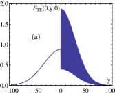
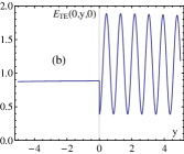
Figure 1: (Color online) (a): $\mathcal{E}_{\text{TE}}(x=0,y,t=0)$ versus $y$. (b): Blowup demonstrating discontinuity in $\mathcal{E}_{\text{TE}}$ due to discontinuity in $\epsilon$ at the interface ($y=0$), $\mathcal{E}_{\text{TE}}(y=0^{-})=\epsilon\,\mathcal{E}_{\text{TE}}(y=0^{+})$. This also demonstrates continuity of $E_{z}$ at the interface.

IV Discussion and conclusions

The parameters used in Gao et al. (2014a) were: $n=1.5$ and $\mu=1$, which implied $\epsilon=2.25$. Furthermore, $\varphi_{\text{i}}=55^{\,\circ}$ and $w_{y_{\text{i}}}/w_{x_{\text{i}}}=2$, as we could read from Fig. 3(b) in Gao et al. (2014a). The value of $\varphi_{\mathrm{i}}$ was close to the Brewster angle $\varphi_{\mathrm{B}}\equiv\arctan n=56.31^{\,\circ}$ for which $R_{\mathrm{TM}}=0$ [$R_{\mathrm{TM}}^{2}(\varphi_{\mathrm{i}}=55^{\,\circ})=1.77847\times 10^{-4}$]. This could be the reason why no reflection was observed in Gao et al. (2014a), see Fig. 2, and would suggest the laser pulse to have TM polarization. In that case, by rotating the light source by $90^{\,\circ}$ around the incident beam axis, the TE polarization would be obtained, for which $R_{\mathrm{TE}}^{2}(\varphi_{\mathrm{i}}=55^{\,\circ})=0.1393$ versus $\epsilon(1+R_{\text{TE}})^{2}=0.8840$ for the refracted beam. The reflected pulse should then be seen along with the incident and refracted ones, see Fig. 3.

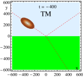
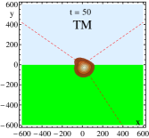
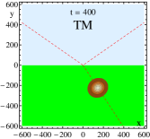
Figure 2: (Color online) Results for $\mathcal{E}_{\text{TM}}(x,y,t)$, spatially averaged over the interference peaks, for $\epsilon=2.25$, $\mu=1$, $\varphi_{\text{i}}=55^{\,\circ}$, $w_{x_{\text{i}}}=50$, $w_{y_{\text{i}}}=100$. No noticeable reflection. The pertinent videos are given in vid1 (our results as above) and in Gao et al. (2014b) (experimental results of Gao et al. (2014a)).

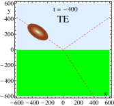
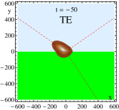
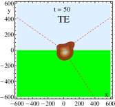
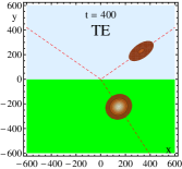
Figure 3: (Color online) As in Fig. 2 but for $\mathcal{E}_{\text{TE}}(x,y,t)$. See vid2 for the video.

In our calculations, based on the dimensionless formulas (16) and (17), for convenience we have chosen the pulse radii to be rather small: $w_{x_{\text{i}}}=50$ and $w_{y_{\text{i}}}=100$. The actual dimensions of the pulses used in Gao et al. (2014a) were much larger but, as we will see, the results in that case are closely related to ours.

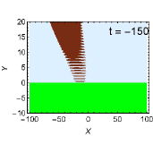
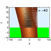
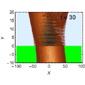
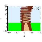
Figure 4: (Color online) Results for $\mathcal{E}_{\text{TE}}(x,y,t)$, $w_{x_{\text{i}}}=20$, and other parameters as in Fig 2.

At any instant $t$, the energy densities $\mathcal{E}_{\text{TM}}(x,y,t)$ and $\mathcal{E}_{\text{TE}}(x,y,t)$ are functions of $x$ and $y$. They can be represented graphically by level contours. If we multiply the pulse radii $w_{x_{\text{i}}}$ and $w_{y_{\text{i}}}$ by some $a>0$, but at the same time multiply by $a$ also $x$, $y$, and $t$, all exponents in (16) and (17) will remain unchanged. Therefore, if furthermore we either drop the cos term (i.e., replace it by its average value zero) or take the extreme values ($\pm 1$) of the cos, the contours in these three cases will scale along with $a$. For example, they will be enlarged $a$ times if $a>1$. During this scaling, the interference peaks shown in Fig. 1 will remain unchanged. This scaling also means that the contours in question for $a\neq 1$ will be the same as those for $a=1$, but one has to multiply by $a$ the numbers associated with $t$ and with the $x$ and $y$ axes (the interference peaks will then get squeezed $a$ times if $a>1$). In particular, this scaling is applicable to the contours shown in Figs. 2 and 3, where we present “macroscopic” results (averaged over the interference peaks by neglecting the cos term).

Notice that for the incident beam, the LHS of (2) gains the factor $a^{-2}$ if $y_{\text{i}}$ and $w_{x_{\text{i}}}$ are multiplied by $a$. This increases the accuracy of (1) if $a>1$. In our case ($a=1$),

$$\lambda_{\text{sw}}=0.8717,\qquad\frac{y_{\text{i}}^{2}(t=-400)}{\hat{y}_{x{\text{i}}}^{2}}\approx 2.6\times 10^{-3},$$ (20)

and the applicability condition (2) implies $a_{\text{min}}\simeq 0.1$ ($w_{x_{\text{i}}\,\text{min}}\simeq 5$).

The laser used in Gao et al. (2014a) was characterized by the wavelength $\lambda_{0}=532$ nm and the pulse duration $\tau=7$ ps. Dividing this $\tau$ by $T_{0}=177.33\times 10^{-5}$ ps to make it dimensionless and using (19) we obtain $w_{y_{\text{i}}}=3352.7$. This leads to $a=w_{y_{\text{i}}}/100\simeq 33.5$, a number by which one has to multiply all numerical values in Figs. 2 and 3, to make them applicable to the experiment described in Gao et al. (2014a).

In Fig. 4 we present the details of the interference peaks evolution. The distance $\lambda_{\text{sw}}$ between the peaks is given by (18) and (20).

A strong validity test for our formulas and calculations was a numerically confirmed continuity of the tangential components of $\mathbf{E}$ and $\mathbf{H}$ across the boundary ($y=0^{\pm}$), and the fact that the total energy was conserved (time independent):

$$\int_{-1000}^{1000}dx\int_{-1000}^{1000}dy\,\mathcal{E}_{\text{TM}}(x,y,t)=7853.982,$$ (21)

for any $t\in[-400,400]$, and exactly the same result for $\mathcal{E}_{\text{TE}}(x,y,t)$, see Figs. 2 and 3. Incidentally, this conservation was also valid for $\mathcal{E}_{\text{TM}}$ and $\mathcal{E}_{\text{TE}}$ spatially averaged over the interference peaks, which can thus be treated as macroscopic energy densities. Equation (21) illustrates high accuracy of the paraxial approximation in our application.

All calculations, figures, and videos were done by using Mathematica.