RD-NMR spectra of the crystal states of the two-dimensional electron gas in a quantizing magnetic field

Abstract

Transport experiments on the two-dimensional electron gas (2DEG) confined into a semiconductor quantum well and subjected to a quantizing magnetic field have uncovered a rich variety of uniform and nonuniform phases such as the Laughlin liquids, the Wigner, bubble and Skyrme crystals and the quantum Hall stripe state. Optically pumped nuclear magnetic resonance (OP-NMR) has also been extremely useful in studying the magnetization and dynamics of electron solids with exotic spin textures such as the Skyrme crystal. Recently, it has been demonstrated that a related technique, resistively-detected nuclear magnetic resonance (RD-NMR), could be a good tool to study the topography of the electron solids in the fractional and integer quantum Hall regimes. In this work, we compute theoretically the RD-NMR line shapes of various crystal phases of the 2DEG and study the relation between their spin density and texture and their NMR spectra. This allows us to evaluate the ability of the RD-NMR to discriminate between the various types of crystal states.

I INTRODUCTION

A two-dimensional electron gas (2DEG) confined into a semiconductor quantum well and subjected to a perpendicular magnetic field $\mathbf{B}$ experiences a great diversity of ground states as the filling factor $\nu=N_{e}/N_{\varphi}$ is varied. Here $N_{e}$ is the number of electrons and $N_{\varphi}=S/2\pi\ell^{2}$ is the Landau level degeneracy with $S$ the 2DEG area and $\ell=\sqrt{\hslash c/eB}$ the magnetic length. Besides the well known (uniform) Laughlin states responsible for the fractional and integer quantum Hall effectsReviewQHE , many nonuniform phases are also possible. These states have spatial modulations of the electronic and/or spin densities. They have been the subject of intense theoretical and experimental work using a variety of techniques over the past 35 years. Famous examples are the Wigner crystal,Wigner ; Wignerrevue the bubble crystals, the quantum Hall stripe stateRevuebulles ; Microwave ; Yoshioka ; Goerbig ; Cotebubble ; Cotestripes and the Skyrme crystal.Sondhi ; Revueskyrmion

Experimental evidence for the crystal phases can be obtained from microwave absorption experimentsMicrowave which detect the gapped phonon mode of the crystal pinned by disorder. In the case of the Skyrme crystal which has an exotic spin texture, optically pumped nuclear magnetic resonance (OP-NMR)Barrett has been particularly useful in measuring the magnetization of the crystal as a function of the filling factor and Zeeman coupling as well as its low-lying collective excitations which involve two gapless (Goldstone) modes.Skyrmecrystal In OP-NMR, the magnetization is obtained by measuring the Knight shift ($K_{s}$) of the ⁷¹Ga nuclei around $\nu=1$ in GaAs/AlGaAs multiple quantum wells. This technique exploits the Fermi contact hyperfine interaction that exists between the magnetic moment of the ⁷¹Ga nuclei in the GaAs quantum wells and the spin of the electrons in the confined 2DEG. A nonzero local spin polarization of the electrons modifies the local magnetic field seen by the nuclei and shift their resonance frequency by an amount $K_{S}$ which is proportional to the electronic spin polarization.

In a related technique: resistively detected nuclear magnetic resonanceDesrat (RD-NMR), the Knight shift of the ⁷⁵As nuclei in the quantum well is obtained from the change in the longitudinal resistance $R_{xx}$ of the 2DEG. This change, $\Delta R_{xx},$ is related to the change in the electronic Zeeman energy which is caused by the coupling via the hyperfine interaction of the average nuclear magnetic moment $\left\langle I_{Z}\right\rangle$ and the electron Zeeman energy $E_{z}\propto\left(B+b_{0}\left\langle I_{Z}\right\rangle\right),$ where $B$ is the external magnetic field and $b_{0}$ is a constant. This technique has been used to study the liquid-solid phase transition of the 2DEG at small filling factor in Landau levels $N=0$ and $N=1.$Gervais ; Tiemann It has also been applied to the Skyrme crystal (or skyrmion liquid) near $\nu=1$ where an anomalous spectral line shape is detected.Desrat ; Gervais ; Gervais2 ; Tracy ; Barrett

The RD-NMR technique has been used recentlyTiemann52 ; Tiemann ; Tiemann2 to study the spatial modulations of the electronic density (or, more precisely, of the spin density) i.e. the topography of the electron solids in the integer and quantum Hall regimes. It is well known (see for example Ref. Cotebubble, ) that the density pattern of a Wigner crystal changes with the Landau level index $N$ because the wave function of an electron in a magnetic field depends on $N$. This change in topography is reflected to some degree in the NMR spectral line shape. Indeed, in experiments, the Wigner crystals detected at small filling factors in Landau levels $N=0$ and $N=1$ show very different RD-NMR spectra.Tiemann In the present work, we want to find out how different the spectral line shape of other crystal states (bubble, stripe, and Skyrme crystals) are from one another and how well the RD-NMR technique can discriminate between them. Is the RD-NMR technique sufficiently sensitive, for exemple, to distinguish between bubble crystals with $2$ or $3$ electrons per site or to separate a bubble crystal from a stripe state? To study this sensitivity, we compare the RD-NMR spectra of several crystal phases where the quasiparticles that crystallize can be electrons, bubbles, skyrmions or the corresponding anti-quasiparticles.

The calculation of the spectral line shape requires a knowledge of the average local spin polarization $\left\langle S_{z}\left(\mathbf{r},z\right)\right\rangle$ along the direction of the applied magnetic field. Here $\mathbf{r}$ is a vector in the plane of the 2DEG and $z$ is in the perpendicular (confining) direction. To compute $\left\langle S_{z}\left(\mathbf{r},z\right)\right\rangle$, we use an equation of motion method developed previously for the study of the Wigner crystal.Cotemethode In this method, the spin polarization is computed from the Hartree-Fock equation of motion of the single-particle Green’s function. This method has the advantage over the Maki-Zotos wave functionMaki that it can easily be adapted to study crystal structures with ferromagnetic or antiferromagnetic order,Wignerspin crystals with more complex spin textures such as meron or skyrmion crystals,Skyrmecrystal or bubble and stripe crystals.Cotebubble ; Cotestripes ; Ettouhami A limitation of this approach, however, is that the Hartree-Fock approximation does not take into account the quantum or thermal fluctuations of the crystals nor the disorder. As previously discussed in the NMR litterature,Desrat ; Gervais2 ; Tracy these effects may alter significantly the NMR spectra. However, by introducing a Gaussian blurring factorTiemann in the calculation of the crystal polarization, it is possible to model the effect of these fluctuations on the spectral line shape. In this work, we limit ourselves to computing the RD-NMR spectra at zero temperature i.e. in the ideal case of frozen crystals. In this regime, the nuclei in the quantum well see an effective magnetic field that depends on their location and so their Knight shift varies spatially. The RD-NMR signal is obtained by summing the Knight-shifted signal of all nuclei as discussed in the next section.

Our paper is organized in the following way. In Secs. II and III, we give a brief summary of the calculation of the RD-NMR spectral line shape for crystal states and of the spin polarization $\left\langle S_{z}\left(\mathbf{r},z\right)\right\rangle$ in the Hartree-Fock approximation. In Sec. IV, we describe the different crystal phases that we include in our study. In Sec. V, we compute the RD-NMR spectra of these crystals and discuss how well the RD-NMR technique allows to discriminate between them. We conclude in Sec. VI.

II CALCULATION OF THE RD-NMR LINE SHAPES

We consider a 2DEG confined in a GaAs/AlGaAs quantum well. The 2DEG is in a perpendicular magnetic field $\mathbf{B}$ that quantizes the kinetic energy into Landau levels. We define $n_{e}$ as the electronic density in the last partially filled Landau level $N$. The filling factor of that level is $\nu=2\pi n_{e}\ell^{2}$. For convenience, we define the dimensionless density $\widetilde{n}_{\alpha}\left(\mathbf{r}\right)$ of each spin specie $\alpha=\uparrow,\downarrow$ in the partially filled Landau level $N$ by

$$\widetilde{n}_{\alpha}\left(\mathbf{r}\right)=\frac{1}{2\pi\ell^{2}}n_{\alpha}\left(\mathbf{r}\right),$$ (1)

where $n_{\alpha}\left(\mathbf{r}\right)$ is the density of electrons with spin $\alpha$. The averaged spin polarization density in the direction of the applied magnetic field is then

$$\left\langle S_{z}\left(\mathbf{r,}z\right)\right\rangle=\frac{\hslash}{4\pi\ell^{2}}m_{z}\left(\mathbf{r}\right)\left|\psi_{\nu}\left(z\right)\right|^{2},$$ (2)

where

$$m_{z}\left(\mathbf{r}\right)=\left\langle\widetilde{n}_{\uparrow}\left(\mathbf{r}\right)\right\rangle-\left\langle\widetilde{n}_{\downarrow}\left(\mathbf{r}\right)\right\rangle,$$ (3)

and $\psi_{\nu}\left(z\right)$ is the wave function of the first bound state of the quantum well which is the only occupied state at sufficiently low temperature. This wave function depends on the exact shape of the quantum well which in turn depends on the potential of the gate used to control the electron density. The notation $\left\langle S_{z}\left(\mathbf{r,}z\right)\right\rangle$ stands for the quantum and thermal averages of the spin density. In this paper, we work at zero temperature and so $\left\langle S_{z}\left(\mathbf{r,}z\right)\right\rangle$ is the ground state average of the spin density.

Following Tiemann et al. (see Supplemental material of Ref. Tiemann, ), we write the spectral function for the RD-NMR signal from the ⁷⁵As nuclei in the quantum well as

$$I_{\nu}\left(f-f_{0}\right) = \frac{A}{WS}\int_{-W/2}^{+W/2}dz\left|\psi_{\text{read}}\left(z\right)\right|^{2}$$

$$\times\int_{S}d\mathbf{r}g\left(f-f_{0}+\beta\left\langle S_{z}\left(\mathbf{r},z\right)\right\rangle\right),$$

where $A$ is a constant and $W$ is the width of the quantum well. In Eqs. (II), $\psi_{\text{read}}\left(z\right)$ is the subband wave function at filling factor $\nu_{\text{read}}$ used to account for the position dependence of the readout sensitivity and $\beta$ is a parameter to be determined experimentally. The function $Ag\left(f-f_{0}\right)$ is the intrinsic line shape for the ⁷⁵As nuclei in the crystal environment (in the absence of the 2DEG). It is assumed to have the Gaussian form

$$g\left(f-f_{0}\right)=e^{-\left(f-f_{0}\right)^{2}/\Gamma^{2}},$$ (5)

where $\Gamma$ is the spectral line shape and $f_{0}$ the resonance frequency. In Eq. (II), it is implicitly assumed that the subband wave function is negligible outside the quantum well. This wave function leads to an asymmetrical broadening of the spectral line shape. The variations of the electronic density in the plane of the well introduce a supplementary inhomogeneous broadening of the line shape.

In our numerical calculation, we compute the wave functions $\psi_{\nu}(z_{i})$ and $\psi_{\text{read}}\left(z_{i}\right)$ in the well at $n_{d}$ points $z_{i}$ and $m_{z}\left(\mathbf{r}_{j}\right)$ at $n_{t}$ points $\mathbf{r}_{j}$ in the unit cell of the crystal. Upon defining

$$\overline{\psi}_{\nu}(z_{i})=\sqrt{\frac{W}{n_{d}}}\psi_{\nu}(z_{i}),$$ (6)

(and a similar relation for $\overline{\psi}_{\text{read}}(z_{i})$) which satisfies

$$\sum_{i=1}^{n_{d}}\left|\overline{\psi}_{\nu}(z_{i})\right|^{2}\approx 1,$$ (7)

we get

$$I_{\nu}\left(f-f_{0}\right) = \frac{A}{Wn_{t}}\sum_{i=1}^{n_{d}}\sum_{j=1}^{n_{t}}\left|\overline{\psi}_{read}(z_{i})\right|^{2}$$

$$\times g\left(f-f_{0}+\zeta n_{d}m_{z}\left(\mathbf{r}_{j}\right)\left|\overline{\psi}_{\nu}\left(z_{i}\right)\right|^{2}\right),$$

where $\zeta$ is now the constant to be found experimentally.

Since $n_{t}$ can be large in Eq. (II), $I_{\nu}\left(f-f_{0}\right)$ is easier to evaluate if we first compute a function giving the probability of occurrence of $m_{z}$. We find the minimal and maximal values of $m_{z}$ in a unit cell, divide the interval between these two values into $n_{b}$ bins of width $\Delta m_{z}$ with middle values $m_{z,k}$ and write $P\left(m_{z,k}\right)$ for the probability of occurrence of $m_{z,k}$. The signal then becomes

$$I_{\nu}\left(f\right) = \frac{A}{W}\sum_{i=1}^{n_{d}}\sum_{k=1}^{n_{b}}P\left(m_{z,k}\right)\left|\overline{\psi}_{read}(z_{i})\right|^{2}$$

$$\times g\left(f-f_{0}+\zeta n_{d}m_{z,k}\left|\overline{\psi}_{\nu}\left(z_{i}\right)\right|^{2}\right),$$

with

$$\sum_{k=1}^{n_{b}}P_{k}=1.$$ (10)

For a uniform state with $m_{z}\left(\mathbf{r}\right)=m_{z},$

$$I_{\nu,\text{uniform}}\left(f\right) = \frac{A}{W}\sum_{i=1}^{n_{d}}\left|\overline{\psi}_{read}(z_{i})\right|^{2}$$

$$\times g\left(f-f_{0}+\zeta n_{d}m_{z}\left|\overline{\psi}_{\nu}\left(z_{i}\right)\right|^{2}\right).$$

Even in this simple case, the line shape is complex since it depends on the form of the confining wave function.

In the experimental setup described in Ref. Tiemann, , the magnetic field is kept fixed. A doping layer provides a finite density of electrons in the well. This density can be modified by changing the potential of a gate allowing the RD-NMR signal to be studied in some range of filling factors. The ionized doping layer, the applied electric field and the finite density of electrons in the well all modify its potential profile and consequently the subband wave functions $\psi_{\nu}\left(z\right)$ and $\psi_{\text{read}}\left(z\right).$ These functions must then be found by solving the Schrödinger-Poisson equations. To fit the experimental RD-NMR signal correctly, these two wave functions must be computed from the exact potential profile of the quantum well at filling factors $\nu$ and $\nu_{\text{read}}.$

In this work, we are interested in studying how a qualitative change in the crystal structure (such as the transition from a Wigner to a bubble crystal with two electrons per site) affects the RD-NMR signal. To isolate the effect of a change in the spin polarization, we assume an ideal situation where the quantum well profile is fixed, i.e. unchanged by a variation of the filling factor. We thus approximate both functions $\psi_{\nu}\left(z\right)$ and $\psi_{\text{read}}\left(z\right)$ by the simple form

$$\psi\left(z\right)=\sqrt{\frac{2}{W}}\cos\left(\frac{\pi z}{W}\right)$$ (12)

which is the first bound state of an infinite quantum well. Our final expression for the RD-NMR spectral line shape is thus

$$I\left(f\right) = \frac{2A}{n_{d}}\sum_{i=1}^{n_{d}}\sum_{k=1}^{n_{b}}P\left(m_{z,k}\right)\cos^{2}\left(\frac{\pi z_{i}}{W}\right)$$

$$\times g\left(f-f_{0}+2\zeta m_{z,k}\cos^{2}\left(\frac{\pi z_{i}}{W}\right)\right).$$

For greater clarity in the figures on this paper, we plot $P\left(m_{z,k}\right)$ as a probability density function $P\left(m_{z}\right)$ instead of as an histogram of values of $m_{z,k}$. We normalize $P\left(m_{z}\right)$ such that:

$$\int_{m_{z,\min}}^{m_{z,\max}}P\left(m_{z}\right)dm_{z}=1.$$ (14)

In our calculations, we discretize the confining wave functions into $n_{d}=200$ points, the unit cell of each crystal into $500\times 500$ points ($n_{t}=250000$) that are further classified into $n_{b}=200$ bins.

III SPIN POLARIZATION DENSITY IN THE HARTREE-FOCK APPROXIMATION

The electronic density in the partially filled level is written as

$$\widetilde{n}_{\alpha}\left(\mathbf{r}\right)=\sum_{\mathbf{G}}\left\langle\rho_{\alpha,\alpha}\left(\mathbf{G}\right)\right\rangle L_{N}^{0}\left(\frac{G^{2}\ell^{2}}{2}\right)e^{-G^{2}\ell^{2}/4}e^{i\mathbf{G}\cdot\mathbf{r}},$$ (15)

where $L_{N}^{0}\left(x\right)$ is an associated Laguerre polynomial and the operator

$$\rho_{\alpha,\beta}\left(\mathbf{G}\right) \equiv \frac{1}{N_{\varphi}}\sum_{X,X^{\prime}}e^{-\frac{i}{2}G_{x}\left(X+X^{\prime}\right)}$$

$$\times\delta_{X,X^{\prime}+G_{y}\ell^{2}}c_{N,X,\alpha}^{\dagger}c_{N,X^{\prime},\beta}.$$

The set of vectors $\left\{\mathbf{G}\right\}$ are the reciprocal lattice vectors of the crystal considered while the set of ground-state average values $\left\{\left\langle\rho_{\alpha,\alpha}\left(\mathbf{G}\right)\right\rangle\right\}$ can be considered as the order parameters of the crystal. They are related to the single-particle Matsubara Green’s function by

$$\left\langle\rho_{\beta,\alpha}\left(\mathbf{G}\right)\right\rangle=G_{\alpha,\beta}\left(\mathbf{G,}\tau=0^{-}\right),$$ (17)

where

$$G_{\alpha,\beta}\left(\mathbf{G,}\tau\right) = \frac{1}{N_{\varphi}}\sum_{X,X^{\prime}}e^{-\frac{i}{2}G_{x}\left(X+X^{\prime}\right)}$$

$$\times\delta_{X,X^{\prime}-G_{y}\ell^{2}}G_{\alpha,\beta}\left(X,X^{\prime},\tau\right)$$

and

$$G_{\alpha,\beta}\left(X,X^{\prime},\tau\right)=-\left\langle Tc_{N,X,\alpha}\left(\tau\right)c_{N,X^{\prime},\beta}^{\dagger}\left(0\right)\right\rangle,$$ (19)

with $T$ the time-ordering operator and $\tau$ the imaginary time. In Eq. (III), the operator $c_{N,X,\alpha}^{\dagger}$ creates an electron in Landau level $N$ with guiding-center index $X$ in the Landau gauge and with spin $\alpha$. Since we consider the filled levels below $N$ as inert (they do not contribute to the spin polarization), we hereafter drop the index $N$ to simplify the notation

The single-particle Green’s function is computed by using an equation of motion methodCotemethode which is generalized to include the spin degree of freedom and the possibility of a spin texture in the plane of the quantum well. The Hartree-Fock equation of motion for $G_{\alpha,\beta}\left(\mathbf{G,}i\omega_{n}\right),$ where $\omega_{n}$ are the Matsubara frequencies, is

$$\left[i\omega_{n}-\left(E_{\alpha}-\mu\right)/\hslash\right]G_{\alpha,\beta}\left(\mathbf{G},\omega_{n}\right)=\delta_{\mathbf{G},0}\delta_{\alpha,\beta}$$ (20)

$$+\frac{1}{\hslash}\sum_{\mathbf{G}^{\prime}\neq\mathbf{G}}U^{H}\left(\mathbf{G-G}^{\prime}\right)e^{-i\mathbf{G}\times\mathbf{G}^{\prime}\ell^{2}/2}G_{\alpha,\beta}\left(\mathbf{G}^{\prime},\omega_{n}\right)$$

$$-\frac{1}{\hslash}\sum_{\mathbf{G}^{\prime}}\sum_{\gamma}U_{\alpha,\gamma}^{F}\left(\mathbf{G-G}^{\prime}\right)e^{-i\mathbf{G}\times\mathbf{G}^{\prime}\ell^{2}/2}G_{\gamma,\beta}\left(\mathbf{G}^{\prime},\omega_{n}\right),$$

with the potentials

$$U^{H}\left(\mathbf{G}\right) = \left(\frac{e^{2}}{\kappa\ell}\right)H\left(\mathbf{G}\right)\left\langle\rho\left(\mathbf{G}\right)\right\rangle,$$ (21)

$$U_{\alpha,\beta}^{F}\left(\mathbf{G}\right) = \left(\frac{e^{2}}{\kappa\ell}\right)X\left(\mathbf{G}\right)\left\langle\rho_{\beta,\alpha}\left(\mathbf{G}\right)\right\rangle,$$ (22)

where $\left\langle\rho\left(\mathbf{G}\right)\right\rangle\equiv\sum_{\alpha}\left\langle\rho_{\alpha,\alpha}\left(\mathbf{G}\right)\right\rangle$ and $\kappa$ is the dielectric constant of the host semiconductor. The non-interacting single-particle energy is given by

$$E_{\alpha}=-\alpha\frac{\left|g^{\ast}\right|\mu_{B}B}{2},$$ (23)

where $g^{\ast}=-0.44$ is the effective $g-$factor of bulk GaAs and $\mu_{B}$ is the Bohr magneton. The Hartree and Fock interactions are defined by

$$H\left(\mathbf{q}\right) = \left(\frac{e^{2}}{\kappa\ell}\right)\frac{1}{q\ell}e^{-q^{2}\ell^{2}/2}\Lambda\left(q\ell\right)\left[L_{N}^{0}\left(\frac{q^{2}\ell^{2}}{2}\right)\right]^{2},$$ (24)

$$X\left(\mathbf{q}\right) = \left(\frac{e^{2}}{\kappa\ell}\right)\sqrt{2}\int_{0}^{\infty}dxe^{-x^{2}}\Lambda\left(x\right)\left[L_{N}^{0}\left(x^{2}\right)\right]^{2}$$

$$\times J_{0}\left(\sqrt{2}xq\ell\right),$$

where $J_{0}\left(x\right)$ is the Bessel function of order zero. Because of the Laguerre polynomial $L_{N}^{0}\left(x\right)$, these interactions depend on the Landau level index $N.$ The function $\Lambda\left(x\right)$ takes into account the finite width of the quantum well. It is defined by

$$\Lambda\left(x\right)=\int_{-\frac{W}{2}}^{+\frac{W}{2}}dz\left|\psi\left(z\right)\right|^{2}\int_{-\frac{W}{2}}^{+\frac{W}{2}}dz^{\prime}\left|\psi\left(z^{\prime}\right)\right|^{2}e^{-x\left|z-z^{\prime}\right|/\ell}$$ (26)

and depends on the magnetic field $B.$ For an ideal 2DEG, $\Lambda\left(x\right)=1.$

Equation (20) is self-consistent and can be solved numerically by successive iterations.Cotemethode A Gaussian blurring $e^{-r^{2}/\sigma^{2}}$ of the density $\widetilde{n}_{\alpha}\left(\mathbf{r}\right)$ can be obtained by multiplying the summand in Eq. (15) by the factor $e^{-\sigma^{2}G^{2}\ell^{2}/4}.$ This blurring can be used to mimic the effects of quantum and thermal fluctuations on the crystal. The parameter $\sigma$ is then adjusted, in this ase, so as to fit the experimental spectra.Tiemann

IV DESCRIPTION OF THE CRYSTAL PHASES

We give now a brief description of the different crystal phases for which we want to compute the NMR spectral line shape. In the Hartree-Fock approximation, even the quantum Hall stripe phase has density modulations along the direction of the stripes and so can be described as a crystal although a very anisotropic one (a face-centered rectangular a large aspect ratio). All these states can by described formally as crystals of some quasiparticle. The quasiparticle can be an electron, an electron bubble, a skyrmion or the corresponding quasi-antiparticles: hole, hole bubble, antiskyrmion. We write $n_{\text{qp}}\left(\mathbf{r}\right)$ for the density of these quasiparticles and define $\nu\in\left[0,2\right]$ as the filling factor of the partially filled level $N$ (the total filling factor is $2N+\nu$). The filled levels are considered as inert. A level with both spin sub-levels filled is unpolarized and so does not contribute to the NMR spectra.

We consider the following phases:

• BC1 ($\nu\leq 0.5$). A bubble crystal, as described in Ref. Cotebubble, , where the quasiparticle at each site is a $M-$electron bubble with spin up. The densities $\widetilde{n}_{\uparrow}\left(\mathbf{r}\right)=n_{\text{qp}}\left(\mathbf{r}\right),\widetilde{n}_{\downarrow}\left(\mathbf{r}\right)=0$ and the spin polarization density is $m_{z}\left(\mathbf{r}\right)=n_{\text{qp}}\left(\mathbf{r}\right).$

• BC2 ($0.5\leq\nu\leq 1$). A bubble crystal where the quasiparticle is a $M-$hole bubble with spin down. The densities $\widetilde{n}_{\uparrow}\left(\mathbf{r}\right)=1-n_{\text{qp}}\left(\mathbf{r}\right),\widetilde{n}_{\downarrow}\left(\mathbf{r}\right)=0$ and $m_{z}\left(\mathbf{r}\right)=1-n_{\text{qp}}\left(\mathbf{r}\right).$

• BC3 ($1\leq\nu\leq 1.5$). A bubble crystal where the quasiparticle is a $M$-electron bubble with spin down. The densities $\widetilde{n}_{\uparrow}\left(\mathbf{r}\right)=1,\widetilde{n}_{\downarrow}\left(\mathbf{r}\right)=n_{\text{qp}}\left(\mathbf{r}\right)$ and $m_{z}\left(\mathbf{r}\right)=1-n_{\text{qp}}\left(\mathbf{r}\right).$

• BC4 ($1.5\leq\nu\leq 2$). A bubble crystal where the quasiparticle is a $M-$hole bubble with spin up. The densities $\widetilde{n}_{\uparrow}\left(\mathbf{r}\right)=1,\widetilde{n}_{\downarrow}\left(\mathbf{r}\right)=1-n_{\text{qp}}\left(\mathbf{r}\right)$ and $m_{z}\left(\mathbf{r}\right)=n_{\text{qp}}\left(\mathbf{r}\right).$

The special case $M=1$ corresponds to the Wigner crystal. The Hartree-Fock Hamiltonian being electron-hole symmetric, $n_{\text{qp}}\left(\mathbf{r}\right)$ is the same function for all four phases. It follows that BC1 and BC4 have the same spectrum and similarly for BC2 and BC3. Moreover, the spectrum for BC2 (or BC4) is obtained from the polarizations $m_{z,k}$ computed for BC1 (or BC3) by replacing $m_{z,k}$ in Eq. (II) by $1-m_{z,k}$.

The description given above for BC1 to BC4 applies with no change to the quantum Hall stripe phases when considered as face-centered rectangular Wigner crystal ($M=1$). In this case, the aspect ratio that minimizes the ground-state energy depends on the Landau level index $N$ and filling factor $\nu$. To distinguish the stripe phases from the bubble crystals, we use for the former the abbreviations SC1 to SC4.

The last phases we consider are the Skyrme crystals. These occur for $\nu$ close to $1$:

• SK1 ($\nu<1$). A crystal where the quasiparticle at each site is an anti-skyrmion of topological charge $Q=-1.$ The densities can be described by $\widetilde{n}_{\uparrow}\left(\mathbf{r}\right)=1-n_{a}\left(\mathbf{r}\right),\widetilde{n}_{\downarrow}\left(\mathbf{r}\right)=n_{b}\left(\mathbf{r}\right).$ They depend on the ratio of the Zeeman coupling to the Coulomb energy $\gamma=\left|g^{\ast}\right|\mu_{B}B/\left(e^{2}/\kappa\ell\right)$ and on the filling factor. The density $m_{z}\left(\mathbf{r}\right)=1-n_{a}\left(\mathbf{r}\right)-n_{b}\left(\mathbf{r}\right)$ while $\widetilde{n}\left(\mathbf{r}\right)=1-n_{a}\left(\mathbf{r}\right)+n_{b}\left(\mathbf{r}\right)=1-n_{\text{qp}}\left(\mathbf{r}\right).$

• SK2 ($\nu>1$). A crystal where the quasiparticle at each site is a skyrmion of topological charge $Q=1.$ The densities $\widetilde{n}_{\uparrow}\left(\mathbf{r}\right)=1-n_{b}\left(\mathbf{r}\right),\widetilde{n}_{\downarrow}\left(\mathbf{r}\right)=n_{a}\left(\mathbf{r}\right)$ and so $m_{z}\left(\mathbf{r}\right)=1-n_{a}\left(\mathbf{r}\right)-n_{b}\left(\mathbf{r}\right)$ and $\widetilde{n}\left(\mathbf{r}\right)=1+n_{\text{qp}}\left(\mathbf{r}\right).$

By electron-hole symmetry, SK1 and SK2 have the same NMR spectrum.Note1 In the Hartree-Fock calculation,Skyrmecrystal the lowest-energy lattice structure for the Skyrme crystal if $\nu$ is not too close to $1$ is a square lattice with two skyrmions of opposite phases per unit cell i.e. the square lattice antiferromagnetic (SLA) phase. It has lower energy than a triangular lattice where all skyrmions have the same phase (TLF). For $\nu$ close to one, a three-sublattice crystal where skyrmions on different sublattice are rotated by $120^{\circ}$ should be the ground state. However, it is difficult to stabilize this phase numerically so that we will only consider the SLA and TLF crystals in our calculation. We remark that, of all the crystal states considered here, SK1 and SK2 are the only ones where $m_{z}\left(\mathbf{r}\right)$ can be locally negative. As we will show, this makes the NMR Skyrme crystal’s spectrum quite different from that of the other crystal states.

V NMR SPECTRA OF THE CRYSTAL STATES

In this section, we compute the RD-NMR spectra of the crystal states described in Sec. IV. Because of the electron-hole symmetry, we can restrict ourselves to the BC1,BC2,SC1,SC2 and SK1 phases. The order parameters for the crystals are calculated for a quantum well of width $W=27$ nm and in a magnetic field $B=6.4$ T as in the experiments.Tiemann We work, however, at zero temperature. We define the Knight shift as the displacement of the peak of the spectrum from the bare resonance frequency $f_{0}.$ At $B=6.4$ T, the ⁷⁵As nucleus has $f_{0}=46.3997$ MHz with a linewidth $\Gamma=1.5$ kHzTiemann . We use this value of $\Gamma$ in our calculations. Figure 4(b) of Ref. Tiemann, gives the expected behavior of the Knight shift of a fully polarized uniform system for filling factors $\nu\in\left[0,1/3\right]$ in Landau level $N=0$. We use this figure to get the constant $\zeta$ that enters Eq. (II). We get $\zeta=16$. Since $\zeta>0,$ a positive spin polarization leads to a negative Knight shift in Eq. (II).

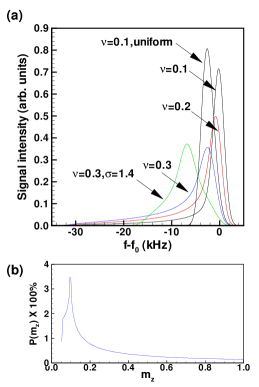
Figure 1: (Color online) (a) RD-NMR spectra for the Wigner crystal phase (BC1) at different filling factors $\nu$ in Landau level $N=0$ with $\sigma=0$ and for $\nu=0.3$ with $\sigma=1.4;$(b) Probability density $P\left(m_{z}\right)$ in the Wigner crystal phase for $\nu=0.3$, $\sigma=0.$

V.1 Phase BC1 with $M=1$ in $N=0$

Figure 1(a) shows the spectra for the BC1 phase with $M=1$ i.e. a Wigner crystal at filling factors $\nu=0.1,0.2,0.3$ in Landau level $N=0.$ These spectra were discussed previouslyTiemann but we reconsider them here for completeness. The spectra are characterized by a single peak and a long tail, absent in the the uniform state, which is due to the large spread in the values of $m_{z}$ in the crystal as shown by the plot of $P\left(m_{z}\right)$ in Fig. 1(b). From Eq. (II), a region of space with a certain $m_{z}$ produces a local shift in frequency of $\approx 2m_{z}\zeta.$ Since $\zeta=16,$ this shift is $32$ kHz for the largest possible value $m_{z}=1$. The function $P\left(m_{z}\right)$ is dominated by the regions of small values of $m_{z}$ so that the Knight shifts in the spectra are small. As $\nu$ increases, the most probable value of $m_{z}$ increases (not shown in the figure) and the Knight shift becomes more negative. At the same time, the maximal intensity of the signal decreases. The most probable value of $m_{z}$ at these filling factors is smaller that the spatially averaged value of $m_{z}$ so that the Knight shift of the crystal is less negative than that of the uniform state. All spectra start at $f-f_{0}=0$ even though the crystal and the liquid have no region with $m_{z}=0.$ This is because the subband wave function term $\overline{\psi}_{\nu}\left(z_{i}\right)$ in Eq. (II) goes to zero at $z=\pm W/2.$

At $\nu=0.3,$ there is an important difference between the theoretical and experimental spectra.Tiemann This is attributed to the fact that the Hartree-Fock approximation for $m_{z}\left(\mathbf{r}\right)$ neglects both quantum and thermal fluctuations. To get a spectra closer to the experimental result, it is necessary to use a finite blurring factor of order $\sigma\approx 1.4$ at $\nu=0.3.$Tiemann As shown in Fig. 1(a), this shifts the peaks to a more negative value and cuts the low-frequency tail.

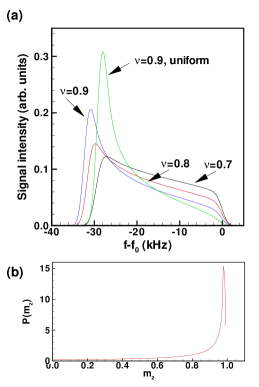
Figure 2: (Color online) (a) RD-NMR spectra for the Wigner crystal phase (BC2) at different filling factors $\nu$ in Landau level $N=0$ with $\sigma=0;$(b) Probability density $P\left(m_{z}\right)$ in the Wigner crystal phase for $\nu=0.8,\sigma=0.$

V.2 Phase BC2 with $M=1$ in $N=0$

Figure 2(a) shows the spectra for the BC2 phase with $M=1$ at filling factors $\nu=0.7,0.8,0.9$ in Landau level $N=0.$ A comparison with Fig. 1(a) shows that the spectra for BC2 are distinctively different from those of BC1. In the plot of $P\left(m_{z}\right)$ in Fig. 2(b), the most probable value for $m_{z}$ is now close to $m_{z}=1$ and so the Knight shift is large. This is also true for the uniform phase. As in BC1, the spread in $m_{z}$ is important and the signal is intense in a large range of frequency shift. In contrast to BC1, however, the maximal $m_{z}$ decreases with decreasing $\nu$ and so does the spread of the signal. The Knight shift becomes less negative with decreasing filling factor because the maximum value of $m_{z}$ decreases with decreasing $\nu$. The most probable value of $m_{z}$ in the BC2 phase is, in contrast to BC1, bigger than that of the uniform state so that the Knight shift in the crystal BC2 state is more negative than in the uniform state.

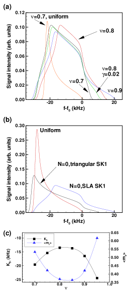
Figure 3: (Color online) RD-NMR spectra in Landau level $N=0$ for: (a) the Skyrme crystal phases (SK1) at different filling factors $\nu$ and for a Zeeman coupling $\gamma=0.015$ (unless indicated otherwise) with $\sigma=0;$ (b) the triangular (TLF) and square (SLA) Skyrme crystals for $\gamma=0.015,\nu=0.9$; (c) Knight shift (measured at the peak position) and spatially averaged polarization $\left\langle m_{z}\right\rangle$ as a function of the filling factor.

V.3 Phase SK1 in $N=0$

Figure 3(a) shows the spectra of the SLA Skyrme crystal SK1 at filling factors $\nu=0.7,0.8,0.9$ in Landau level $N=0$ for a Zeeman coupling $\gamma=g^{\ast}\mu_{B}B/\left(e^{2}/\kappa\ell\right)=0.015$ and at $\nu=0.8$ for $\gamma=0.02.$ For comparison, we include the spectrum of the uniform state at $\nu=0.7$ for $\gamma=0.015.$ The polarization $S_{z}=\left(\nu_{\uparrow}-\nu_{\downarrow}\right)/\nu$ is shown as a function of $\nu$ and $\gamma$ in Fig. 1 of Ref. Skyrmecrystal, . (In that calculation, the well width was taken to be zero but taking $W=27$ nm does not change much that result.) That Hartree-Fock calculation of $S_{z}$ gives a fairly accurate description of the magnetization of the Skyrme crystal observed in NMR experiments.Barrett As Fig. 3(a) shows, the spectrum for the Skyrme crystal is different from that of the Wigner crystal [compare Fig. 2(a) and Fig. 3(a)] or the uniform state. For the Skyrme crystal, there is large frequency range of positive Knight shift which is due to the spatial regions of reversed spin (negative $m_{z}$) in the skyrmion’s texture. In the Wigner crystal, there is no spin texture and $m_{z}\left(\mathbf{r}\right)$ is always positive. For $\nu\rightarrow 1,$ the skyrmion’s size and so the number of reversed spins increases meaning that the spatial regions of positive Knight shift increase too. The regions of positive shift decrease with increasing Zeeman coupling $\gamma$ since that coupling decreases the skyrmion’s size. Another important difference between the spectrum of the Wigner and the Skyrme crystals is that the former is independent of $\gamma.$

We compare the spectra of different Skyrme crystal lattices at $\nu=0.9$ in Fig. 3(b). The SLA and triangular Skyrme crystals in $N=0$ are evaluated at $\gamma=0.015.$ They have a spatially averaged polarization $m_{z}=0.42$ and $m_{z}=0.77$ respectively. The Knight shift is larger for the triangular lattice because of the regions of higher polarization but the positive Knight shift extends to higher frequencies for the SLA structure which has more reversed spins. The Skyrme crystal for a perfect 2DEG is not expected to be the ground state for $N>0.$ Indeed, in $N=1,2$ we were not able to stabilize a Skyrme crystal even for a Zeeman coupling as small as $\gamma=0.0001.$ With a large number of iterations, the solution converges towards a triangular Wigner crystal of holes (BC2) with no spin texture [its spectrum is shown in Fig. 4(b)]. This is consistent with a recent experimentTiemann2 where no Skyrme crystal are detected in $N=1$ around $\nu=1$ a finite temperature. The low-temperature phase of the 2DEG in this case seems to be a Wigner crystal of holes (type BC2 with $M=1$). The difference in the line shapes of BC2 crystals for $N=0$ and $N=1$ [compare Fig. 2(a) with Fig. 4(b) arises because of the difference in the electronic wave functions of the two Landau levels as we explain in more detail below.

Figure 3(c) shows the Knight shift measured at the position of the peak in the spectrum of Fig. 3(a) and the spatially averaged polarization $m_{z}$ as a function of the filling factor $\nu.$ For $\nu<1,$ the uniform state has $m_{z}=1.$ As can be seen by comparing the two curves, the relation between the Knight shift measured in this way and the average magnetization is not exactly linear (as is the case for zero-width uniform 2DEG).

The spectra that we gave in this section apply to an ideal situation where the Skyrme crystals are frozen. With thermal fluctuations, the line shapes may be very different. At finite temperature, one must know the exact regime where the experiment is carried on i.e. the Skyrme’s crystal dynamics.Barrett ; Sinova ; Villares ; Gervais2 ExperimentsBarrett ; Desrat close to $\nu=1$ have measured an anomalous line shape for the Skyrme crystal that our simple ground-state calculation cannot reproduce. in fact, it has even been suggested that the dispersive line shape found experimentally may be inconsistent with the usual model of RD-NMR where the signal is due solely to a hyperfine-induced increase of the electronic Zeeman energy.Tracy

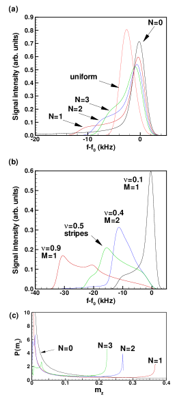
Figure 4: (Color online) RD-NMR spectra for: (a) the BC1 phase with $M=1$ (Wigner crystal) at filling factor $\nu=0.1$ in Landau levels $N=0,1,2,3$ and for the uniform phase at $\nu=0.1;$ (b) the BC1, SC1 and BC2 phases in Landau level $N=1$ at different filling factors; (c) probability density $P\left(m_{z}\right)$ for the same phases as in (a). The function $P\left(m_{z}\right)$ for $N=0$ extends to $m_{z}=1$ (not shown on the graph).

V.4 Phases BC1,BC2 and SC1,SC2 in Landau levels $N>0$

The Laguerre polynomial $L_{N}^{0}\left(x\right)$ that enters the calculation of the density as well as the Hartree and Fock potentials causes these functions to change with the Landau level index. In $N=0,$ the density for a bubble crystal with $M=1$ has a Gaussian profile centered at each lattice site. For $N>0$ and $M=1,$ the density profile has the form of a ring centered on each lattice site. A new ring is added each time $M$ increases with the exception of the last bubble phase with $M=N+1$ in Landau level $N.$ In this case, a peak is added at the center of the existing $M$ rings (see Fig. 2 of Ref. Cotebubble, ).

We compare the spectra of the $M=1$ BC1 phase for $N=0,1,2,3$ at $\nu=0.1$ in Fig. 4(a). The corresponding probability densities $P\left(m_{z}\right)$ are shown in Fig. 4(c). The most probable density is the minimal density which increases with $N$ while its probability decreases with $N.$ Consequently, the Knight shift in Fig. 4(a) becomes more negative with $N$ but the peak intensity in the spectral line shape decreases with $N$. The next contribution to these spectra comes from the ring. At fixed $\nu,$ the diameter of the ring increases with $N$ while $m_{z}$ in the ring decreases. This behavior is reflected in the spectra shown in Fig. 4(a): the frequency and the intensity of the shoulder in the spectrum increases with $N$ since, as the ring expands, it covers a greater area. For comparison, we include in Fig. 4(a) the spectrum of the uniform phase at $\nu=0.1$ which is independent of $N.$ The peak in the density of the crystal for $N=0,M=1$ produces a long tail in its spectrum that is absent of the spectrum of a $M=1$ crystal in higher Landau levels.

Figure 4(b) shows the spectra of several phases in Landau level $N=1:$ the BC1 crystals with $M=1$ ($\nu=0.1$) and $M=2$ ($\nu=0.4$), the stripe phase SC1 at $\nu=0.5$ and the BC2 crystal with $M=1$ at $\nu=0.9.$ The stripe phase is not present in $N=1$ in the HFA but appears in DMRG calculation.Yoshioka On the contrary, the $M=2$ bubble crystal is present in HFA but not in DMRG. The transition from $M=1$ to $M=2$ is predicted to occur at $\nu=0.36$ in the HFA. The phase diagram obtained in DMRG is richer than that of the HFA because it contains the fractional quantum Hall states and other correlated liquid states. In contrast to the HFA, it predicts some form of stripe state in $N=0$ (whose structure is however different from the stripe state found in higher Landau levels) and a stripe state in $N=1$ when $\nu\in\left[0.38,0.47\right]$ whose structure is similar to the stripe state in higher Landau levels predicted by the HFA. Up to now, only the $M=1$ BC1 phase has been detected experimentally.Tiemann2 The long tail in the $N=1,M=2$ phase, like that of the Wigner crystal with $N=0,M=1$ is due to the peak in density. This makes its spectrum different from that of the other phases in $N=1$. The spectra of the different phases in $N=1$ are quite different and their detection should allow the unambiguous identification of the corresponding phases.

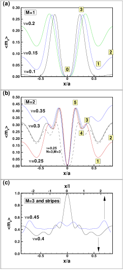
Figure 5: (Color online) Traces of the spin density $m_{z}\left(\mathbf{r}\right)$ along $x$ for $y=0$ and at different filling factors in $N=2$ for the : (a) $M=1$ bubble crystals; (b) $M=2$ bubble crystals; (c) $M=3$ bubble crystals (bottom $x$ axis) and stripe phase (top $x$ axis). The numbers identify a region that contributes to a peak in the function $P\left(m_{z}\right)$ shown in Fig. 6(a). Here $a$ is the lattice spacing and $\ell$ is the magnetic length. The dashed curve in (b) shows the magnetization trace for $N=3,M=2$ at $\nu=0.25.$

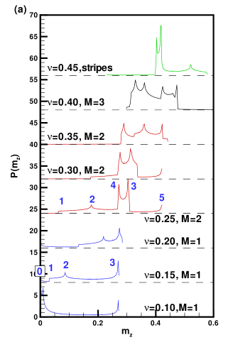
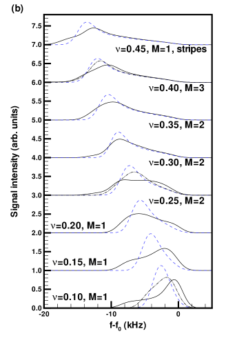
Figure 6: (Color online) (a) Probability density $P\left(m_{z}\right)$ for some BC1 and SC1 phases in Landau level $N=2$ at different filling factors $\nu<0.5.$ Each curve is offset by $8$ from the one below for clarity. This offset must be deducted from the value of $P\left(m_{z}\right)$; (b) corresponding RD-NMR spectra for the crystal phases in (a) (full black curve) and for the uniform phases (dashed blue curves). Each curve is offset by 1 from the one below for clarity. The intensity is in arbitrary units, but the same for all curves. The dashed-dotted curves are the spectra of the crystal phases with a blurring factor $\sigma=1.4.$

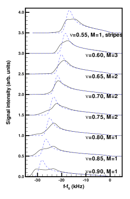
Figure 7: (Color online) RD-NMR spectra for the BC2 crystal phase (full black curve) and uniform phase (blue dashed curves) in Landau level $N=2$ for filling factor $0.5<\nu<1.$ The curves are offset by $0.5$ for clarity. The intensity is in arbitrary units, the same for all curves.

We now consider Landau level $N=2.$ Figure 1(a) of Ref. Cotebubble, shows the phase diagram of the 2DEG in Landau level $N=2$ for $0\leq\nu\leq 0.5.$ The density pattern for each phase (BC1 and SC1) is shown in Fig. 2 of that reference. In the HFA, there is a transition at $\nu=0.22$ from $M=1$ to $M=2$ and at $\nu=0.37$ a second transition to $M=3$. The stripe phase SC1 is reached after $\nu=0.43.$ These numbers are for a perfect 2DEG. They are slightly modified when $W$ is finite as is the case here. Figure 5 shows the polarization $m_{z}\left(\mathbf{r}\right)$ along $x$ for $y=0$ in the bubble and stripe phases at different values of the filling factors. The corresponding functions $P\left(m_{z}\right)$ and line shapes $I_{\nu}\left(f\right)$ are shown in Fig. 6(a) and Fig. 6(b) respectively. The bubble crystals and stripes of holes BC2, SC2 follow the same phase diagram than BC1, SC1 but in reverse order, i.e., the crystal of electrons at $\nu<0.5$ is replaced by a crystal of holes at filling factor $1-\nu$ and $m_{z}$ is replaced by $1-m_{z}$ in the calculation of the line shape. The spectra of the phases BC2, SC2 are shown in Fig. 7. The density $m_{z}$ being bigger in the hole phases than in the electron phases, the Knight shift is larger in the former than in the latter.

As $\nu$ increases, the radius of the ring in the $M=1$ bubble crystal increases. The transition to the $M=2$ crystal occurs when rings from adjacent sites just touch. At this point, there is an abrupt transition to the $M=2$ bubble crystal which has two rings. As $\nu$ increases further, these two rings expands and there is again an abrupt transition to the $M=3$ bubble crystal when the outer rings from adjacent sites just touch. The $M=3$ bubble crystal has two rings and one central maximum on each site. From Fig. 5, as $\nu$ increases, the average value of the magnetization increases and there are more oscillations in $m_{z}\left(\mathbf{r}\right)$ and consequently more structure in $P\left(m_{z}\right).$ In each case, there is one oscillation with a large value of $\Delta m_{z}\left(\mathbf{r}\right)$ and other smaller ones. In the stripe phase, the oscillations are much less pronounced than in the crystal phases. As regards its NMR spectrum, this phase is close to that of the uniform phase.

In Fig. 5, the numbers above the lines for $\nu=0.15$ and $\nu=0.25$ identify the regions in $m_{z}\left(\mathbf{r}\right)$ that are responsible for a peak in the corresponding plot of $P\left(m_{z}\right)$ shown in Fig. 6(a). We see in Fig. 5(b) that, in comparison with $M=1,$ the $M=2$ bubble crystal has one extra ring which adds the extra peaks numbered $3$ and $4$ in Fig. 6(a) for $\nu=0.25.$

The spectral line shape of the BC1, SC1 crystals changes with increasing $\nu$ and is different from that of the uniform phase. The signal from the $M=2$ crystal at $\nu=0.25$ looks different from that of the $M=1$ crystal at $\nu=0.1$ but is not very different from the $M=1$ crystal at $\nu=0.2.$ Even though the functions $P\left(m_{z}\right)$ shown in Fig. 6(a) are quite different, many of the peaks in $P\left(m_{z}\right)$ are too close in $m_{z}$ to be resolved in the spectra. For example, the peaks numbered $3$ and $4$ in Fig. 6(a) (for $\nu=0.25,M=2$) are spaced by $\Delta m_{z}=0.025.$ This leads to peaks separated by $\Delta f=0.8$ kHz in the line shape. This separation is smaller than the linewidth $\Gamma=1.5$ kHz considered in our calculation. It follows that most of the interesting features in $P\left(m_{z}\right)$ are lost in the integrated signal $I_{\nu}\left(f\right)$ (not considering the extra complication due to confining wave function). The signal from the $M=3$ BC1 crystal, however, is different from that of the $M=1,2$ crystal and the stripe phase. It has a characteristic long low frequency tail (not visible in Fig. 6(a) but it is finite up to $m_{z}=1$ and in Fig. 6(b) it extends to $f-f_{0}=-32$ kHz). As we mentioned above, this phase may not be present in the ground state according to DMRG calculations. We expect the same conclusions to hold for Landau levels $N>2$ since there are more oscillations in bubbles with higher values of $M$ and these oscillations are smaller in amplitude [see the traces for $M=2,\nu=0.25$ and $N=2,3$ in Fig. 5(b)]. Except in some range of $\nu$ (fort $\nu=0.3-0.35,$ for example) most spectra are sufficiently different from that of the corresponding uniform state to allow a discrimination between the uniform and crystal states. Unfortunately, it does not seem possible to infer the number of electrons in each bubble crystal from its spectrum alone when $N\geq 2$ (with the exception of $M=N+1$) since the distinguishing features in the density are lost in the integrated signal. It may also be difficult to differentiate between the $M=2$ crystal and the stripe phase as their spectra are not dramatically different. Moreover, the oscillations are small in the stripe phase and the corresponding NMR spectrum is close to that of the uniform state. One marked difference between the $M=2$ and $M=1$ spectra, however, is that the maximal Knight shift (in absolute value) is larger in the former than in the latter. Indeed, as Fig. 6(a) shows, the maximum value of $m_{z}\left(\mathbf{r}\right)$ increases discontinuously with $M.$

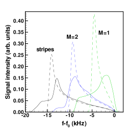
Figure 8: (Color online) $N=2$ RD-NMR spectra (full curves) for the $M=1$ and $M=2$ bubble crystals at $\nu=0.15$ and $\nu=0.3$ and for the stripe phase at $\nu=0.45$ calculated with a linewidth $\Gamma=0.5$ kHz. The dashed curves are the spectra of the corresponding uniform phases.

At some filling factors in $N=2$, the difference between the crystal and liquid spectra is small and may be washed out by fluctuations. We give some examples of that in Fig. 6(b) where the dashed-dotted curve represent the crystal phases calculated with a Gaussian blurring factor $\sigma=1.4$ which is the value necessary in $N=0$ to make the calculated spectrum agrees with the experimental result according to Ref. Tiemann, . We see that, with the exception of $\nu=0.1,$ the spectra for $\nu=0.25$ and $\nu=0.4$ are almost identical with those of the corresponding uniform states. We checked that the value of $\sigma$ that brings the crystal spectrum identical with that of the uniform state for the Wigner crystal at $\nu=0.1$ in $N=0,1,2$ are $\sigma=4.5,4.0,3.5$ respectively. The crystal state is thus more fragile in higher Landau levels.

VI CONCLUSION

We have presented in this paper a study of the RD-NMR spectra of various crystal phases that can theoretically exist as ground states of the 2DEG in the quantum Hall regime. In Landau levels $N=0,1$, Wigner crystal, bubble crystal, stripe phase and Skyrme crystal (when present) produce distinct RD-NMR line shapes that should allow their unambiguous experimental identification. In higher Landau levels, the RD-NMR spectra are not so distinct with the exception of the $M=N+1$ bubble crystal. In these levels, crystal and uniform states can be distinguished but it would be difficult to differentiate between the Wigner, bubble (with $M>1$ and $M<N+1$) and stripe phases.

Our calculation assumed the ideal case of a frozen solid at zero temperature. As shown beforeTiemann ; Tiemann2 , thermal fluctuations will render the crystal spectra closer to that of the uniform state. This will not help the differentiation of the different phases in $N\geq 2$ since the small difference in the spectra will probably be washed out unless the temperature is very small.

The NMR spectra would be more discriminating with a stronger hyperfine coupling between the electron gas and the nuclei or with a reduced linewidth $\Gamma$ but these parameters are fixed by the quantum well. We have used the value $\Gamma=1.5$ kHz in all our calculationsTiemann but, as a test, we show in Fig. 8 the spectra for the $N=2$ stripe phase at $\nu=0.45$ and the $N=2,M=1,2$ bubble crystals at $\nu=0.15$ and $\nu=0.3$ with a smaller linewidth $\Gamma=0.5$ kHz. The distinction between the solid and uniform phases is much clearer [compare with Fig. 6(b)]. Apart from the important difference in the range of the Knight shift for crystal with different values of $M$, the spectra for the $M=2$ crystal and the stripe phase still have a similar shape.

In a real experimental situation, the filling factor is tuned by changing the potential on a gate in the GaAs/AlGaAs quantum well. This modifies the shape of the confining wave function that enters the calculation of the NMR spectra. We have considered this wave function as fixed, but our calculation can easily take this effect into account (by solving the Schrödinger-Poisson equations) if an exact description of the quantum well is given.