Distortion Limited Amplify-and-forward Relay Networks and the $\epsilon$-critical Phase Transition

Abstract

We study amplify-and-forward (AF) relay networks operating with source and relay amplifier distortion, where the distortion dominates the noise power. The diversity order is shown to be $0$ for fixed-gain (FG) and $1$ for variable-gain (VG) if distortion occurs at the relay; if distortion occurs only at the source, the diversity order will be $1$ for both. With $\epsilon_{\beta}=N_{0}/\eta_{\beta}$ ($N_{0}$ the noise power, $\eta_{\beta}$ the distortion power at node $\beta\in\{S,R\}$, the source or relay), we demonstrate the emergence of what we call an $\epsilon$-critical signal-to-noise plus distortion ratio (SNDR) threshold (a threshold that emerges when $\min\{\epsilon_{\beta}\}$ becomes small) for both forwarding protocols. We show that crossing this threshold in distortion limited regions will cause a phase transition (a dramatic drop) in the network’s outage probability. Thus, small reductions in the required end-to-end transmission rate can have significant reductions in the network’s outage probability.

I Introduction

Relaying will play a vital role in future vehicular-to-vehicle (V2V) communications due to the diversity gains it can offer, and its ability to extend a network’s coverage area [1, 2, 3, 4]. AF relaying is particularly attractive for low latency requirements [5], which will be prevalent in V2V communications.

OFDM systems are known to have a large peak-to-average power ratio (PAPR) making them much more susceptible to distortion due to nonlinearities. Combining OFDM with channel fading can cause even larger PAPRs in the received signal at the relay of OFDM networks, which may lead to more pronounced nonlinear distortion. Although nonlinear effects are common in such networks, there is minimal literature pertaining to them. In [6], the outage probability of a two-hop cooperative OFDM VG relay system in the presence of relay nonlinearities is approximated, while [7] focuses on the bit-error rate of such a system when nonlinear amplifications occur at the source. Outage and symbol error rate expressions are obtained for FG systems subject to nonlinear amplification at the relay in [8]. Outage probability expressions and power allocation strategies are obtained in [9] and [10], respectively, for two-way AF networks with nonlinearities at the relay.

Contributions of this work

To the best of the authors’ knowledge, there has been no work that specifically focuses on the effects of distortion limitation within the context of relaying systems. In this paper, we assess such effects. In particular, we show that:

1. For distortion limited FG networks:

   1. relay distortion results in a diversity order of $0$.

   2. no relay distortion (but still source distortion) results in a diversity order of $1$.

2. For distortion limited VG networks, the diversity order is always $1$.

3. For distortion limited FG and VG networks, a critical outage probability SNDR threshold emerges. If the networks operate below this threshold, outage will occur almost surely. However, crossing the threshold will cause a phase transition (a dramatic drop) in the network’s outage probability. Thus, small changes in the required end-to-end transmission rate can have significant implications for the network’s outage probability.

It is worth mentioning that point 1) contrast with known results when no distortion is present, [11], where it is shown that the diversity order is $1$ for both forwarding schemes.

We use $x\sim y$ to denote that $x$ is asymptotically equivalent to $y$, and $x:=y$ and $y=:x$ to denote that $x$ is defined to be equal to $y$.

II System Model

Consider a two-hop, time-division duplexing (TDD) AF OFDM network operating over $n$ subcarriers, Fig. 1. The impulse response for hop $\beta\in\{1,2\}$ is assumed to be $l$ taps long, quasi-static, and given by the time-domain (TD) vector

$$\bar{H}_{\beta}=\sqrt{\frac{n}{l}}\frac{\left[\bar{h}_{\beta 0}\;\;\bar{h}_{\beta 1}\;\;\cdots\;\;\bar{h}_{\beta,l-1}\right]^{T}}{\left|\left[\bar{h}_{\beta 0}\;\;\bar{h}_{\beta 1}\;\;\cdots\;\;\bar{h}_{\beta,l-1}\right]\right|},$$ (1)

where the $i$th entry of $\bar{H}_{\beta}$ corresponds to the $i$th channel tap and $\tilde{h}_{\beta i}$, $i\in\{0,\dots,l-1\}$, are i.i.d. zero-mean complex Gaussian (ZMCG) random variables with total variance $\mu_{\beta}$. After taking the unitary Fourier transform (FT) of $\bar{H}_{\beta}$, the frequency response for the $k$th subcarrier of hop $\beta\in\{1,2\}$ is given by $h_{\beta k}\sim\mathcal{CN}\left(0,\mu_{\beta}\right)$, $k\in\{1,\dots,n\}$.

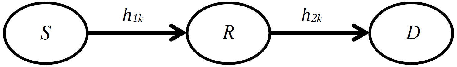
Figure 1: Relay network. $h_{ik}$ is the channel coefficient for $i$th hop on $k$th subcarrier.

The relaying protocol takes place over two time slots. The first time-slot, amplification model, and second time-slot are detailed in the following subsections.

II-A First Time Slot

Node $S$ constructs an OFDM symbol vector comprised of $n$ symbols, which we denote by the frequency-domain (FD) vector $X_{S}=[x_{S{1}},\ldots,x_{S{n}}]^{T}$, where $\sigma_{S}^{2}:=\mathbb{E}[|x_{S{k}}|^{2}]$. It is assumed that the symbol $x_{S{k}}$ is chosen uniformly and independently from a quadrature phase-shift keying (QPSK) constellation.

II-A1 Cyclic Prefix Insertion and Removal

The vector $X_{S}$ is processed with an inverse FT, after which a cyclic prefix (CP) of suitable length is appended to mitigate IBI. We assume that CP insertion and removal is performed entirely at the source and destination; i.e., not at the relay. Consequently, the CP must be more than $2l$ sample periods in length to mitigate IBI. The TD OFDM block at $S$ is then given by

$$\bar{X}_{S,cp}=\left[\bar{x}_{S,n-2l-1}\;\cdots\;\bar{x}_{S,n-1}\;\right.\left.\bar{x}_{S,0}\;\bar{x}_{S,1}\cdots\;\bar{x}_{S,n-1}\right]^{T},$$ (2)

where $\bar{x}_{S,i}$ is the $(i+1)$th entry of $\bar{X}_{S}:=\mathbf{F}^{-1}{X}_{S}$ (the inverse FT of ${X}_{S}$).

II-A2 Source Transmission

The source has a maximum transmit power constraints, $\mathcal{P}_{max,S}$. To ensure this constraint is not exceeded, $S$ passes its TD waveform through a soft envelope limiter (SEL) (see [12, eq. (38)]). The output of the SEL in the TD given that the input is the $(k+1)$th element of $\bar{X}_{S}:=\mathbf{F}^{-1}{X}_{S}$ is

$$\bar{y}_{Sk}=\min\left\{\sqrt{\mathcal{P}_{maxS}},|\bar{x}_{Sk}|\right\}\exp\left(i\arg\bar{x}_{Sk}\right).$$ (3)

By considering Bussgang’s theorem [12], and provided the number of subcarriers is sufficiently large, the $k$th subcarrier frequency-domain (FD) output of the SEL can be written as

$$y_{Sk}=\zeta_{S}x_{Sk}+d_{Sk},$$ (4)

where $d_{Sk}\sim\mathcal{CN}\left(0,\eta_{S}\right)$ is uncorrelated with $x_{Sk}$, and $\zeta_{S}$ and $\eta_{S}$ are obtained from [12, eq. (42)]

$$\zeta_{\beta}=1-e^{-\frac{p_{max\beta}}{\sigma_{\beta}^{2}}}+\sqrt{\frac{\pi p_{max\beta}}{4\sigma_{\beta}^{2}}}\mathrm{erfc}\left(\frac{p_{max\beta}}{\sigma_{\beta}^{2}}\right)$$ (5)

$$\eta_{\beta}=\sigma_{\beta}^{2}\left(1-e^{-\frac{p_{max\beta}}{\sigma_{\beta}^{2}}}\right)-\zeta_{\beta}^{2}\sigma_{\beta}^{2}.$$ (6)

By noting that the SEL’s input power is exponentially distributed, the average transmit power, $\mathcal{P}_{S}$, at $S$ is obtained from

$$\mathcal{P}_{\beta}=\intop_{0}^{\infty}\frac{\min\{x,\mathcal{P}_{max,\beta}\}e^{-\frac{x}{\sigma_{\beta}^{2}}}}{\sigma_{\beta}^{2}}dx=\sigma_{\beta}^{2}\left(1-e^{-\frac{p_{max\beta}}{\sigma_{\beta}^{2}}}\right).$$ (7)

The received signal at the relay on the $k$th subcarrier is then

$$y_{Rk}=h_{1k}\zeta_{S}x_{Sk}+v_{Rk}+h_{Ak}d_{Ak},$$ (8)

where $v_{Rk}\sim\mathcal{CN}\left(0,N_{0}\right)$ is a $k$th subcarrier noise term.

II-B Relay Amplification Model

Once $y_{Rk}$, (8), has been received, the relay performs the amplification process and then transmits the resultant signal. This process takes place over two distinct steps.

Step One

The relay applies the amplification factor $G_{\alpha k}$ to the $k$th subcarrier, where $\alpha\in\{FG,VG\}$ denotes whether FG or VG is employed. For FG, $G_{\alpha k}$ is given by

$$G_{FGk} = \sqrt{\frac{\sigma_{R}^{2}}{p_{A}\mu_{A}+N_{0}}};$$ (9)

where $\sigma_{R}^{2}$ is the average input power to the SEL at the relay. For VG, $G_{\alpha k}$ is given by

$$G_{VGk}=\sqrt{\frac{\sigma_{R}^{2}}{p_{A}|h_{Ak}|^{2}+N_{0}}}.$$ (10)

Note, (9) is independent of $k$. However, to aid exposition, we refrain from removing the subscript $k$.

Step Two

The relay passes the amplified TD waveform through an SEL to limit the maximum transmit power to $\mathcal{P}_{maxR}$. As an immediate consequence of the central limit theorem, this TD signal converges in distribution to a stationary ZMCG variable with variance $\sigma_{R}^{2}$ as the number of subcarriers grows large. This allows us to apply Bussgang’s theorem at the relay too.

It is important to note, however, that convergence to a stationary ZMCG variable for FG is also contingent on there being a sufficient number of channel taps. To understand this, consider the extreme scenario in which the channels are flat across all subcarriers; i.e., they have a single tap response. Furthermore, note that quasi-static fading has been considered, so the channel are fixed for a single OFDM TD block. For this, the subcarrier responses will be independent of their indices, i.e., $h_{1i}=h_{1j}$ $\forall\;i,j$. For $h_{1i}=h_{1}$ $\forall$ $i$, this allows us to write the TD waveform at the relay’s SEL as

$$Y_{R}(t)=\frac{1}{\sqrt{n}}\sum_{k=1}^{n}e^{\frac{i2\pi kt}{n}}G_{FGk}\left(h_{1}\zeta_{S}x_{Sk}+v_{Rk}+h_{1}d_{Sk}\right).$$ (11)

Because the gains are fixed and independent of $k$, and the channel coefficients are quasi-static, $Y_{R}(t)$ will approach a ZMCG variable with conditional variance

$$\mathbb{V}\left[Y_{R}\left(t\right)|h_{1}\right]=\left(\frac{\sigma_{R}^{2}}{\mathcal{P}_{S}\mu_{1}+N_{0}}\right)\left(\mathcal{P}_{S}\left|h_{1}\right|^{2}+N_{0}\right),$$ (12)

where conditioning is performed to account for the channel’s quasi-static nature. Thus, we will not have the requirement for Bussgang’s theorem that the input to the SEL be a stationary ZMCG variable with variance $\sigma_{R}^{2}$. In particular, it will be a function of $h_{1}$. However, as the number of channel taps grows, $h_{1i}$ and $h_{1j}$, $i\neq j$, will become increasingly decorrelated and the averaging performed by the inverse FT in (11) will remove the dependence of $Y_{R}(t)$’s conditional variance on the instantaneous realizations of $h_{1k}$, and $Y_{R}(t)$ will approach a stationary ZMCG random variable with conditional variance $\sigma_{R}^{2}$. Of course, in practice the number of channel taps will be finite. However, from heuristic observations we find that $16$ or more channel taps allows for very accurate modeling of FG systems using Bussgang’s theorem. Note, it was shown [13] that a particular $20$MHz non-line-of-sight environment would have as many as $40$ taps in its channel impulse response.

As with before, we can write the FD output of the SEL as

$$x_{Rk}=\zeta_{R}G_{\alpha k}y_{Rk}+d_{Rk},$$ (13)

where $\zeta_{R}$ is obtained from (5) and $d_{Rk}$ is uncorrelated with $y_{Rk}$ and well approximated by a ZMCG random variable with variance $\eta_{R}$ obtained from (6). The average transmit power on each subcarrier at the relay is given by $\mathcal{P}_{R}$ (see (7)).

II-C Second Time Slot

By assuming channel reciprocity, which follows from the TDD nature of the channel, and that the entire relaying process has taken place within the coherence time of the channel, the received signal on the $k$th subcarrier at the destination is

$$y_{Dk}=h_{2k}x_{Rk}+v_{Dk},$$ (14)

where $v_{Dk}\sim\mathcal{CN}(0,n_{0})$ is the noise term on the $k$th carrier at $D$. Note, to obtain (14) the destination must first remove the CP from the received TD block and perform an FT on this block. The $k$th element of the FT’s output vector will then be given by (14). The instantaneous per-subcarrier SNDR is then

$$\lambda_{\alpha,k}=\frac{\sigma_{S}^{2}\zeta^{2}_{S}|h_{1k}|^{2}G_{\alpha,k}^{2}\zeta_{R}^{2}|h_{2k}|^{2}}{|h_{2k}|^{2}\left(G^{2}_{\alpha,k}\zeta^{2}N_{0}+\eta_{S}|h_{1k}|^{2}G_{\alpha,k}^{2}\zeta_{R}^{2}+\eta_{R}\right)+N_{0}}.$$ (15)

III Outage Probability - Distortion Limitation

We begin by considering general noise and distortion conditions with the aim of quantifying the effects that distortion limitations have on performance.

III-A Outage Probability Derivation

The per-subcarrier outage probability is defined to be

$$P_{o,\alpha} := \mathbb{P}\left[\lambda_{\alpha,k}\leq\gamma_{th}\right],$$ (16)

where $\gamma_{th}$ is an SNDR protection threshold. For FG, the solution to (16) is given in [8, eq. (16)] when only relay distortion occurs. For VG, the outage probability when only relay distortion occurs can be obtained as a special case of the two-way network given by [9, eq. (26)]. This is done by considering the limit as the transmit power at the destination node tends to zero (i.e., when the two-way network studied in [9] becomes one-way). For VG, (16) then becomes

$$P_{o,VG}\!\!\!\!\! = \!\!\!\!\!\left\{\begin{array}[]{cc}\!\!1\!\!-\!\!2e^{-Q}\sqrt{R}K_{1}\left(2\sqrt{R}\right)\!,&\!\!\!\!\zeta_{R}^{2}\sigma_{R}^{2}\!>\!\gamma_{th}\eta_{R}\!\!\\ 1,&\!\!\!\!\zeta^{2}_{R}\sigma_{R}^{2}\!\leq\!\gamma_{th}\eta_{R}\!\!\\ \end{array}\right.,$$ (19)

when distortion occurs only at the relay; where $K_{1}\left(\cdot\right)$ is the first order modified Bessel function of the second kind,

$$R:=\frac{\gamma_{th}}{\bar{\Sigma}_{1}\bar{\Sigma}_{R}}\left(1+\frac{\bar{\Sigma}_{2}\gamma_{th}}{\bar{\Sigma}_{R}}\right);\quad Q:=\frac{\gamma_{th}}{\bar{\Sigma}_{R}}\left(1+\frac{\bar{\Sigma}_{2}}{\bar{\Sigma}_{1}}\right);$$

and

$$\bar{\Sigma}_{1}:=\frac{\mathcal{P}_{S}\mu_{1}}{N_{0}},\;\bar{\Sigma}_{2}:=\frac{\mathcal{P}_{R}\mu_{2}}{N_{0}},\;\bar{\Sigma}_{R}:=\bar{\Sigma}_{2}-\frac{(1+\gamma_{th})\mu_{2}}{\epsilon_{R}}$$ (20)

are the average first and second hop SNRs, and average critical second-hop SNR, respectively, and $\epsilon_{R}:=N_{0}/\eta_{R}.$ The outage probability solution when only relay distortion occurs can be extended to the scenario where source distortion occurs by making the substitution $\gamma_{th}\to\gamma_{th}\mathcal{P}_{S}/(\sigma^{2}_{S}\zeta^{2}_{S}-\gamma_{th}\eta_{S})$, where $\sigma^{2}_{S}\zeta^{2}_{S}-\gamma_{th}\eta_{S}\leq 0$ implies outage will occur surely.

III-B Distortion Limited Performance

Let us consider $P_{o,\alpha}$ when distortion power dominates noise power. To do this, we make the following assumptions:

1. the source power is proportional to the relay power,

2. the power clipping ratios, $\mathcal{P}_{max,\beta}/\sigma_{\beta}^{2}$, are fixed.

With these assumptions, $\zeta_{\beta}$ becomes fixed and we can write

$$\mathcal{P}_{R}=\tilde{\mathcal{P}}_{R}\mathcal{P}_{S},\;\;\sigma_{\beta}^{2}=\tilde{\sigma}_{\beta}^{2}\mathcal{P}_{S}\;\;\mathrm{and}\;\;\eta_{\beta}=\tilde{\eta}_{\beta}\mathcal{P}_{S},$$ (21)

where $\tilde{\mathcal{P}}_{R},\;\tilde{\sigma}_{R}^{2},\;\tilde{\eta}_{\beta}\in\mathbb{R}^{+}$ are proportionality constants.

Because of our assumptions, analyzing the system when it is distortion limited (i.e., when $\max\{\eta_{S},\eta_{R}\}\gg N_{0}$) is identical to analyzing the system in the high transmit power regime. Consequently, we study the first order behavior of $P_{o,\alpha}$ as $\mathcal{P}_{S}\to\infty$. With $\tilde{\sigma}_{S}^{2}\zeta^{2}_{S}-\gamma_{th}\tilde{\eta}_{S}>0$, for FG (16) is given to first order by [8, Eq. (16)]

$$\!\!\!\!\!\!P_{o,FG}\!\sim\!\left(1\!-\!e^{\!\!\!-\frac{\tilde{\eta}_{R}\gamma_{th}}{\left(\tilde{\sigma}_{S}^{2}\zeta^{2}_{S}-\gamma_{th}\tilde{\eta}_{S}\right)\tilde{\sigma}_{R}^{2}\zeta_{R}^{2}}}\right)\!+\log\left(\mathcal{P}_{S}\right)\!\left(g_{FG}\mathcal{P}_{S}\right)^{-1}\!;\\$$ (22)

while for VG, from (19), it is given by

$$P_{o,VG}\sim\left(g_{VG}\mathcal{P}_{S}\right)^{-1};$$ (23)

where $g_{\alpha}(\alpha\in\left\{FG,VG\right\}$ ) is given by

$$\!\!\!\!g_{FG}\!\!\! = \!\!\!\frac{\tilde{\mathcal{P}}_{R}\tilde{\sigma}_{R}^{2}\zeta_{R}^{2}\mu_{B}\left(N_{0}\gamma_{th}\left(\tilde{\eta}_{R}+\tilde{\sigma}_{R}^{2}\zeta_{R}^{2}\right)\right)^{-1}}{\exp\left({-\frac{\tilde{\eta}_{R}\gamma_{th}}{\tilde{\sigma}_{R}^{2}\zeta_{R}^{2}\left(\tilde{\sigma}_{S}^{2}\zeta^{2}_{S}-\gamma_{th}\tilde{\eta}_{S}\right)}}\right)},$$ (24)

$$\;\;\!\!\!\!g_{VG}\!\!\! = \!\!\!\frac{\left(\tilde{\sigma}_{R}^{2}\zeta_{R}^{2}\!-\!\frac{\tilde{\eta}_{R}\gamma_{th}}{\left(\tilde{\sigma}_{S}^{2}\zeta^{2}_{S}-\gamma_{th}\tilde{\eta}_{S}\right)}\right)\mu_{1}\mu_{2}}{N_{0}\gamma_{th}\left(\mu_{1}+\tilde{\mathcal{P}}_{R}\mu_{2}\right)}$$ (25)

for FG and VG, respectively, and describes the vertical shift associated with the asymptotic outage probability curves. Assuming $\sigma^{2}_{S}\zeta^{2}_{S}-\gamma_{th}\eta_{S}>0$, the diversity of FG relaying is

$$l_{FG}:=-\lim_{\mathcal{P}_{S}\to\infty}\left(\frac{\log P_{o,FG}}{\log\mathcal{P}_{S}}\right)=\left\{\begin{array}[]{cc}0&\tilde{\eta}_{R}\neq 0\\ 1&\tilde{\eta}_{R}=0\end{array}\right.;$$ (28)

while for VG, it is independent of $\tilde{\eta}_{R}$, and given by

$$l_{VG}:=-\lim_{\mathcal{P}_{S}\to\infty}\left(\frac{\log P_{o,VG}}{\log\mathcal{P}_{S}}\right)=1.$$ (29)

We find that, for a fixed power clipping ratio and assuming $\sigma^{2}_{\beta}\zeta^{2}_{\beta}-\gamma_{th}\eta_{\beta}>0$, relay distortion only affects the diversity for FG, while distortion at the source has no affect on the diversity for either forwarding strategy. Note, the terms $g_{\alpha}$ are affected by the distortion. These observations contrast with known results for FG and VG relaying [11] where it was observed that, without nonlinear distortion at the source or relay, the diversity gains for FG and VG are always $1$.

IV The $\epsilon$-critical Phase Transition

To explain the results that were seen above (e.g., why VG asymptotically outperforms FG with relay distortion, or why the first order expansion of the FG outage probability is lower bounded by the bracketed term of (LABEL:eq:asymPoFG)), we will now define the ratio between the noise power and the distortion power at node $\beta$ to be $\epsilon_{\beta}$; i.e.,

$$\epsilon_{\beta}:=\frac{N_{0}}{\eta_{\beta}},\;\beta\in\{S,R\}.$$ (30)

Furthermore, we also define $\epsilon_{\star}$ to be

$$\epsilon_{\star}=\min_{\beta}\{\epsilon_{\beta}\}$$ (31)

With (30) and (31), for FG we can write (15) as

$$\lambda_{FG,k}\!=\!\frac{{\tilde{\sigma}_{S}^{2}\zeta_{S}^{2}\tilde{\sigma}_{R}^{2}\zeta_{R}^{2}|h_{1}|^{2}}\Big{/}{\left(\mu_{1}\max\{\eta_{\beta}\}\right)}}{a_{FG}\!+\!l_{FG}\epsilon_{\star}\!+\!q_{FG}{\epsilon_{\star}}^{2}}$$ (32)

where $a_{FG}=\frac{\tilde{\eta}_{R}}{\max\{\tilde{\eta}_{\beta}\}}+\frac{\tilde{\sigma}_{R}^{2}\zeta_{R}^{2}|h_{1}|^{2}\tilde{\eta}_{S}}{\max\{\tilde{\eta}_{\beta}\}\mu_{1}}$, $l_{FG}=\frac{1}{\left|h_{2k}\right|^{2}}\!+\!\frac{\tilde{\mathcal{P}}_{R}}{\mu_{1}}$, and $q_{FG}=\frac{\tilde{\eta}_{R}}{\mu_{1}\left|h_{2k}\right|^{2}}$; and for VG (15) becomes

$$\!\lambda_{VG,k}\!=\!\frac{{\tilde{\sigma}_{S}^{2}\zeta_{S}^{2}\tilde{\sigma}_{R}^{2}\zeta_{R}^{2}}\Big{/}{\max\{\eta_{\beta}\}}}{a_{VG}\!+\!l_{VG}\epsilon_{\star}\!+\!q_{VG}\epsilon_{\star}^{2}}.$$ (33)

where $a_{VG}=\frac{\tilde{\eta}_{R}}{\max\{\tilde{\eta}_{\beta}\}}+\frac{\tilde{\sigma}_{R}^{2}\zeta_{R}^{2}\tilde{\eta}_{S}}{\max\{\tilde{\eta}_{\beta}\}}$, $l_{VG}=\frac{1}{\left|h_{2k}\right|^{2}}+\frac{\tilde{\mathcal{P}}_{R}}{|h_{1k}|^{2}}$, and $q_{FG}=\frac{\tilde{\eta}_{R}}{\left|h_{1k}\right|^{2}\left|h_{2k}\right|^{2}}$.

Our goal is to analyze the system as $\epsilon_{\star}\to 0$. This can be done by letting $N_{0}\to 0$ or $\max\{\eta_{\beta}\}\to\infty$. With the fixed power clipping ratio assumptions, both approaches will yield

$$\!\!\lambda_{FG,k}\!\sim\!\frac{\tilde{\sigma}_{S}^{2}\zeta_{S}^{2}\tilde{\sigma}_{R}^{2}\zeta_{R}^{2}|h_{1}|^{2}}{\left(\tilde{\eta}_{R}\!+\!\frac{\tilde{\sigma}_{R}^{2}\zeta_{R}^{2}\tilde{\eta}_{S}|h_{1}|^{2}}{\mu_{1}}\right)\mu_{1}},\lambda_{VG,k}\!\sim\!\frac{\tilde{\sigma}_{S}^{2}\zeta_{S}^{2}\tilde{\sigma}_{R}^{2}\zeta_{R}^{2}}{\tilde{\eta}_{R}\!+\!{\tilde{\sigma}_{R}^{2}\zeta_{R}^{2}\tilde{\eta}_{S}}}.$$ (34)

From (34), we see that the asymptotic behavior of $\lambda_{VG,k}$ is necessarily deterministic, while for $\lambda_{FG,k}$ it is deterministic only if source distortion exists and the relay is distortion free. Crucially, both of these terms are independent of $\mathcal{P}_{S}$, which is why the outage probability for FG is lower bounded (i.e., does not decay asymptotically) when relay distortion occurs, while for VG it always decays to $0$. Furthermore, the lower bound on the FG outage probability, i.e., the bracketed term of (LABEL:eq:asymPoFG), is simply the CDF of $\lambda_{FG,k}$’s asymptotic behavior.

IV-A The $\epsilon$-critical Phase Transition and SNDR thresholds

We will now show for FG and VG that an $\epsilon$-critical phase transition (a phase transition arising for small $\epsilon_{\star}:=\min_{\beta}\{\epsilon_{\beta}\}$) will occur about a critical value of $\gamma_{th}$, which we call the $\epsilon$-critical SNDR threshold. We will then calculate the outage probability drop that occurs during this phase transition.

For FG, consider the outage probability of $\lambda_{FG,k}$’s asymptotic behavior (see (34)), which can be manipulated into

$$\mathbb{P}\left[\frac{\tilde{\sigma}_{R}^{2}\zeta_{R}^{2}|h_{1}|^{2}}{\mu_{1}\tilde{\eta}_{R}}\left(\tilde{\sigma}_{S}^{2}\zeta_{S}^{2}-\gamma_{th}\tilde{\eta}_{S}\right)\leq\gamma_{th}\right].$$ (35)

From (35), we see that if $\tilde{\sigma}_{S}^{2}\zeta_{S}^{2}/\tilde{\eta}_{S}\leq\gamma_{th}$ outage will occur almost surely as $\mathcal{P}_{S}\to\infty$ (i.e., $\epsilon_{\star}\to 0$); otherwise, it will go to the bracketed term of (LABEL:eq:asymPoFG). Consequently, we expect to observe a phase transition in the distortion limited region for the FG network at the critical $\gamma_{th}$ point

$$\gamma_{th,c}^{(FG)}=\tilde{\sigma}_{S}^{2}\zeta_{S}^{2}/\tilde{\eta}_{S}.$$ (36)

A similar event occurs for VG, but because the asymptotic behavior of $\lambda_{VG,k}$ is necessarily deterministic, the critical $\gamma_{th}$ point follows immediately from (34), and is given by

$$\gamma_{th,c}^{(VG)}={\tilde{\sigma}_{S}^{2}\zeta_{S}^{2}\tilde{\sigma}_{R}^{2}\zeta_{R}^{2}}\Big{/}\left({\tilde{\eta}_{R}+{\tilde{\sigma}_{R}^{2}\zeta_{R}^{2}\tilde{\eta}_{S}}}\right).$$ (37)

We call (36) and (37) the $\epsilon$-critical SNDR thresholds.

Figs. 2 and 3 show plots of $P_{o,\beta}$ as a function of $\gamma_{th}$ for FG and VG, and the $\epsilon$-critical values of $\gamma_{th}$ (vertical dashed lines), (36) and (37). From these figures, the phase transitions can be seen as $\mathcal{P}_{S}/N_{0}$ grows (i.e., as $\epsilon_{\star}$ becomes small). These figures also contain numerically generated plots (circular markers), and plots of the first order expansions (expanded about $\gamma_{th}=0$) of the outage probability functions (diagonal dashed lines). The first order expansions will be used below to establish the size of the outage probability drop occuring as $\gamma_{th,c}^{(\alpha)}$ is crossed.

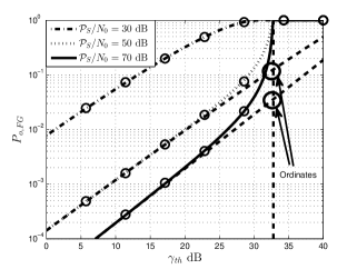
Figure 2: $P_{o,VG}$ as function of $\gamma_{th}$. As $\mathcal{P}_{S}/N_{0}$ increases, $\epsilon_{\star}$ decreases and the phase transition becomes visible. We set $\mu_{1}=\mu_{2}=N_{0}=1$, $\mathcal{P}_{max,S}/\sigma_{S}^{2}=5$, $\mathcal{P}_{max,R}/\sigma_{R}^{2}=8$, $l=32$ taps. Lines - theoretical results. Markers - Monte Carlo simulations with $N=512$. Vertical dashed line is $\gamma_{th,c}^{(FG)}$, (36). Straight diagonal dashed lines - (38). Ordinates given (asymptotically) by (40).

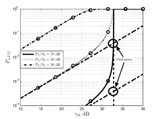
Figure 3: $P_{o,VG}$ as function of $\gamma_{th}$. As $\mathcal{P}_{S}/N_{0}$ increases, $\epsilon_{\star}$ decreases and the phase transition becomes visible. $\mu_{1}=\mu_{2}=N_{0}=1$, $\mathcal{P}_{max,S}/\sigma_{S}^{2}=\infty$, $\mathcal{P}_{max,R}/\sigma_{R}^{2}=5$, $l=32$ taps. Lines - theoretical results. Markers - Monte Carlo simulations with $N=512$. Vertical dashed line - $\gamma_{th,c}^{(VG)}$, (37). Straight diagonal dashed lines - (39). Ordinates given (asymptotically) by (41).

IV-B Outage Drop about the $\epsilon$-critical SNDR Threshold

To establish the size of the outage probability drop about $\gamma_{th,c}^{(\alpha)}$, we begin by calculating the first order expansions of the outage expressions at $\gamma_{th}=0$. For FG, this is given by

$$P_{o,FG}\!\sim\!Z\gamma_{th}\!\left[\bar{\Sigma}_{2}+{\Sigma_{1}\mu_{2}}/{\epsilon_{R}}+\right.\\ \left.\!\left(1\!+\!\bar{\Sigma}_{1}\right)\left(1\!-\!2C\!-\!\log\left[Z\gamma_{th}\left(1\!+\!\bar{\Sigma}_{1}\right)\right]\right)\right]\!,$$ (38)

where $C$ is the Euler-Mascheroni constant and $Z=1\Big{/}\left({\frac{\sigma_{S}^{2}\zeta_{S}^{2}\mu_{1}}{N_{0}}\frac{\sigma_{R}^{2}\zeta_{R}^{2}\mu_{2}}{N_{0}}}\right)$. For VG, it is given by

$$P_{o,VG}\sim{Z\gamma_{th}\left(1-2C+\bar{\Sigma}_{1}+\bar{\Sigma}_{2}-\log\left(Z\gamma_{th}\right)\right)}.$$ (39)

We now use (38) and (39) to understand the phase transitions observed in Figs. 2 and 3. This is done by evaluating them at the $\epsilon$-critical SNDR threshold ((36) or (37)), which will give us the ordinates illustrated in these figures and indicate the outage probability drop that should be expected as the $\epsilon$-critical threshold is crossed. For FG, with $\tilde{\eta}_{S}\neq 0$, the ordinate is given to leading order about $\epsilon_{\star}=0$ by

$$\mathrm{Ord}_{FG}\sim\frac{\epsilon_{\star}\max\{\tilde{\eta}_{\beta}\}}{\tilde{\eta}_{S}\tilde{\sigma}_{R}^{2}\zeta_{R}^{2}\mu_{2}}\left(\frac{\mu_{2}}{\epsilon_{R}}+\log\left(\frac{\tilde{\eta}_{S}\tilde{\sigma}_{R}^{2}\zeta_{R}^{2}\mu_{2}}{\epsilon_{\star}\max\{\tilde{\eta}_{\beta}\}}\right)\right);$$ (40)

while for VG, it is given by

$$\mathrm{Ord}_{VG}\sim\!\frac{\epsilon_{\star}^{2}\max\{\tilde{\eta}_{\beta}\}}{a_{VG}\mu_{1}\mu_{2}}\log\left(\frac{a_{VG}\mu_{1}\mu_{2}}{\epsilon_{\star}^{2}\max\{\tilde{\eta}_{\beta}\}}\right).$$ (41)

IV-C A Discussion of the $\epsilon$-critical Phase Transition

We will now elucidate some observations made in the above subsections. First, from (36) and (37), we find that

$$\gamma_{th,c}^{(FG)}-\gamma_{th,c}^{(VG)}={\tilde{\sigma}_{S}^{2}\zeta_{S}^{2}\tilde{\eta}_{R}}\Big{/}\left({\tilde{\eta}_{S}\tilde{\eta}_{R}+\tilde{\sigma}_{R}^{2}\zeta_{R}^{2}\tilde{\eta}_{S}}\right).$$ (42)

Consequently, $\gamma_{th,c}^{(VG)}\leq\gamma_{th,c}^{(FG)}$, where equality is maintained when the relay is distortion free. It follows that if $\gamma_{th,c}^{(VG)}<\gamma_{th}<\gamma_{th,c}^{(FG)}$ FG will outperform VG in distortion limited regions. This is the only point at which distortion limited FG networks appear favorable over distortion limited VG networks. Moreover, if $\gamma_{th}$ belongs to this interval, by considering the FG outage probability lower bound (the bracketed term of (LABEL:eq:asymPoFG)), FG will outperform VG at most by the factor

$$1-\exp\left({-{\tilde{\eta}_{R}\gamma_{th,c}^{(VG)}}\Big{/}{\left(\tilde{\sigma}_{S}^{2}\zeta^{2}_{S}-\gamma_{th}\tilde{\eta}_{S}\right)\tilde{\sigma}_{R}^{2}\zeta_{R}^{2}}}\right).$$

Turning our attention to the outage probability drop that occurs about $\gamma_{th,c}^{(\alpha)}$, from (40) and (41) we find that the ordinate of the drop scales at best (i.e., when $\epsilon_{R}=\infty$) like $O\left(-\epsilon_{S}\log\epsilon_{S}\right)$ for FG, while it always scales like $O\left(-\epsilon_{\star}^{2}\log\epsilon_{\star}^{2}\right)$ for VG. Consequently, much larger outage probability drops should be expected for the VG. Furthermore, when $\epsilon_{R}\neq\infty$, (40) becomes $O(1)$; i.e., it becomes independent of $\epsilon_{\star}$. This makes sense from our observation that the outage probability for FG is lower bounded when distortion occurs at the relay.

V Conclusion

We studied AF relay networks employing nonlinearities at the source and relay while operating in distortion limited regions. It was shown that distortion at the source would not affect the diversity order, while distortion at the relay would affect this, but only for FG. We then revealed a critical SNDR threshold for both FG and VG. We termed this threshold the $\epsilon$-critical SNDR threshold. Finally, it was shown that crossing the threshold in distortion limited scenarios would cause a phase transition in the outage probability of the network.

References

- [1] J. Laneman, D. Tse, and G. Wornell, “Cooperative Diversity in Wireless Networks: Efficient Protocols and Outage Behavior,” Information Theory, IEEE Transactions on, vol. 50, pp. 3062 – 3080, dec. 2004.
- [2] A. Chandra, C. Bose, and M. Bose, “Wireless Relays for Next Generation Broadband Networks,” Potentials, IEEE, vol. 30, pp. 39 –43, march-april 2011.
- [3] Y. Yamao and K. Minato, “Vehicle-roadside-vehicle relay communication network employing multiple frequencies and routing function,” in Wireless Communication Systems, 2009. ISWCS 2009. 6th International Symposium on, pp. 413–417, IEEE, 2009.
- [4] J. Zhao, T. Arnold, Y. Zhang, and G. Cao, “Extending drive-thru data access by vehicle-to-vehicle relay,” in Proceedings of the fifth ACM international workshop on VehiculAr Inter-NETworking, pp. 66–75, ACM, 2008.
- [5] Y. Yang, H. Hu, J. Xu, and G. Mao, “Relay Technologies for WiMAX and LTE-Advanced Mobile Systems,” Communications Magazine, IEEE, vol. 47, no. 10, pp. 100–105, 2009.
- [6] C. Alexandre and R. Fernandes, “Outage Performance of Cooperative Amplify-and-Forward OFDM Systems with Nonlinear Power Amplifiers,” in Signal Processing Advances in Wireless Communications (SPAWC), 2012 IEEE 13th International Workshop on, pp. 459–463, 2012.
- [7] T. Riihonen, S. Werner, F. Gregorio, R. Wichman, and J. Hamalainen, “BEP Analysis of OFDM Relay Links with Nonlinear Power Amplifiers,” in Wireless Communications and Networking Conference (WCNC), 2010 IEEE, pp. 1–6, 2010.
- [8] D. Simmons and J. Coon, “OFDM-based Nonlinear Fixed-Gain Amplify-and-Forward Relay Systems: SER Optimization and Experimental Testing,” in Networks and Communications, IEEE European Conference on, pp. 1–5, June 2014.
- [9] D. Simmons and J. Coon, “Two-way OFDM-based Nonlinear Amplify-and-Forward Relay Systems,” 2015.
- [10] D. Simmons and J. Coon, “OFDM-based Nonlinear Amplify-and-Forward Relay Systems: Power Allocation,” in Networks and Communications, IEEE European Conference on, pp. 1–5, June 2015.
- [11] M. O. Hasna and M.-S. Alouini, “A Performance Study of Dual-hop Transmissions with Fixed Gain Relays,” in Acoustics, Speech, and Signal Processing, 2003. Proceedings.(ICASSP’03). 2003 IEEE International Conference on, vol. 4, pp. IV–189, IEEE, 2003.
- [12] D. Dardari, V. Tralli, and A. Vaccari, “A Theoretical Characterization of Nonlinear Distortion Effects in OFDM Systems,” Communications, IEEE Transactions on, vol. 48, no. 10, pp. 1755–1764, 2000.
- [13] N. Moraitis, A. Kanatas, G. Pantos, and P. Constantinou, “Delay Spread Measurements and Characterization in a Special Propagation Environment for PCS Microcells,” in Personal, Indoor and Mobile Radio Communications, 2002. The 13th IEEE International Symposium on, vol. 3, pp. 1190–1194 vol.3, Sept 2002.