Optical Properties of Rydberg Excitons and Polaritons

Abstract

We show how to compute the optical functions when Rydberg Excitons appear, including the effect of the coherence between the electron-hole pair and the electromagnetic field. We use the Real Density Matrix Approach (RDMA), which, combined with Green’s function method, enables one to derive analytical expressions for the optical functions. Choosing the susceptibility, we performed numerical calculations appropriate to a Cu₂0 crystal. The effect of the coherence is displayed in the line shape. We also examine in details and explain the dependence of the oscillator strength and the resonance placement on the state number. We report a good agreement with recently published experimental data.

I Introduction

Since the 1980s Rydberg atoms, in which the valence electron is in a state of high principal quantum number $n\gg 1$, have been extensively studied. They have exaggerated atomic properties including dipole-dipole interactions that scale as $\sim n^{4}$ and radiative lifetimes proportional to $n^{2}$. Another important property of the Rydberg states is the large orbital radius, and hence dipole moment $\sim n^{2}$. The natural consequence of the large dipole moment featured by the Rydberg atoms is the large interaction between two of them - one is able to observe dipole-dipole interactions between atoms on the $\mu$ scale. Another consequence of the incredibly large dipole moment is an exaggerated response to external fields Gallagher . Due to a small admixing of the Rydberg state with the ground one, the atoms experience long-range and large interactions while keeping a long lifetime in a quantum superposition, which is very useful for creating qubits, so Rydberg atoms are well suited to applications in quantum information processing. The idea of using dipolar Rydberg interactions to implement the Rydberg blockade bases on the fact that in an ensemble of atoms with long-range dipolar interactions between them, only one atom can be excited at given time. This ’dipole blockade’ has now been observed for two single atoms positioned at macroscopic distances Weide . Rydberg interaction between distanced atoms is used to implement one or two-qubit quantum gates of high fidelity qinf . Coupling of Rydberg states results in d.c. Kerr effect which is six order of magnitude greater then in conventional Kerr. This result has great impact on development of high-precision electric field sensors and other nonlinear optical devices nat . Rydberg atoms are also applied in single-microwave-photon counters what is especially promising in high precession measurements in quantum optics ver . On this wide background of potential applications established in quantum optics and atomic physics demonstration of gigant Rydberg excitons in cooper oxide (Hofling , Kazimierczuk ) is a great step toward studies that are out of the reach in atomic physics, f.e. Rydberg excitons, due to their smaller energies, need lower magnetic field to mimick hydrogen atoms in white-draft stars fried or they are promising candidate for creating Bose-Einstein condensat in solid Stolz .

The phenomenon of excitons and its consequences on the optical spectra of semiconductors, intensively studied over the decades, obtained a new impulse when the so-called Rydberg excitons have been detected in a natural crystal of copper oxide found at the Tsumeb mine in Namibia Hofling , Kazimierczuk . In the simplest picture the exciton (we have in mind the so-called Wannier exciton) is modelled as a hydrogen-like atom, composed from the electron and the hole, interacting via the Coulomb potential screened by the semiconductor dielectric constant. The materials, where Wannier excitons occur, show optical spectra where the transition states, related to the principal quantum number $n$, are observed. In most previously studied materials, like, for example, GaAs, only few excited excitonic states ($n=1,2,3$) were detected, which was caused by the small excitonic binding energy (in the order of a few meV, as in GaAs), and dissipative processes. Therefore the discovery reported in Ref. Kazimierczuk , where the analysis of the spectra revealed spectral absorption lines associated with the formation of excitons that have principal quantum numbers as large as n = 25, provoke a new situation in the condensed matter optics. Many problems as, for example, the light-matter interaction when the excitons with such large quantum numbers are present, will expect new description. Excitonic spectra of highly excited Rydberg excitons observed recently resemble that of a hydrogen atom consisting of a Rydberg series but even if the hydrogen picture of the exciton seems to be very simple, then, the calculations with eigenfunctions related to $n=25$ would be not trivial. The standard description needs to be revised do to the fact that a size of the exciton is much larger then the wavelenght of light used to create it Hofling . There are many factors, as, for example, the band structure, the temperature, the laser power, the dissipative processes, which should be included in the theoretical description.

Here we neither enter into the analysis of the experiment nor in the calculations of the band structure. We propose a method, which gives a simple expression for the optical functions, taking into account excitonic states of arbitrary order which allows one to obtain theoretical spectra and to analyze the experimental ones. The method is based on the Real Density Matrix Approach and uses Green’s function method to solve the Schrödinger-like equations which are typical for this approach. The method will also give insight into the aspect of polaritons, which are closely related to the excitonic states. The RDMA, initiated by the works by Stahl et al. see, for example, StB87 , CBT96 , was very succsessful in describing optical properties of semiconductors for energies near the fundamental gap, where the excitons are relevant. This approach also solved the old ABC problem (for example, Birman82 -Agran2009 ), at least for the cases with a few excitonic states CBT96 . In what follows we focuss the attention on the optical spectra of Cu₂O. As it follows by the analysis of crystal symmetry, the lines related to odd angular momentum exciton number $\ell=1,3,..$ are observed Thewes . The dominant role play the $P$-excitons (the so-called yellow series), but also excitonic states with higher than $\ell=1$ angular momentum (for example, the $F$- excitons with $\ell=3$ and $H$- excitons with $\ell=5$) were observed in one-photon absorption spectra of high-quality cuprous oxide. Our method gives not only the energy eigenvalues, but also the line shapes of the optical functions, from which we have chosen the susceptibility. The presented theory explains many peculiar characteristics of Rydberg excitons such as deviations from $n^{-3}$ law of oscillator strengths and $n^{-2}$ law for the excitonic energies and gives the polariton dispersion relation. Using anisotropic effective masses, we show the energy splitting of the $P$, $F$, and $H$ excitons. Our numerical results are in agreement with measurements obtained recently in the outstanding experiments performed by Kazimierczuk et al. Kazimierczuk and Thewes et al. Thewes .

It is believed that the observation of Rydberg excitons allows one to open a new field in condensed matter spectroscopy. For highly excited Rydberg excitons in Cu₂O the scale is of over 1$\mu$m Tizei so the application of solid state huge-size excitons as all-optical switching, mesoscopic single-photon devices or their implementation to construction of quantum gates influences the development of new experimental technics. Additionally, it is interesting to note that the excitonic approach toward the old idea of Rydberg atoms is example how the development of one field inspires the others.

Our paper is organized as follows. In the section II, we briefly recall the basic equations of the RDMA approach and derive expressions for the interband susceptibility. Next, in section III, the derived expression is analyzed for the case of Cu₂O crystal. In section IV, the derived expression for the susceptibility is used to obtain the polariton dispersion relation of the considered cuprous oxide crystal. In section V we show the impact of the effective masses anisotropy on the calculated optical properties. In section VI the method of calculating the susceptibility and the polariton dispersion in terms of an appropriate Green’s function is presented. In section VII the results for the absorption spectra are presented and discussed. The comparison of obtained results with experimental data and a brief overview of optimizing procedure is included.We close with final remarks in section VIII.

II Density matrix formulation

Having in mind the experiments by Kazimierczuk et al. Kazimierczuk , we will compute the linear optical response of a semiconductor platelet to a plain electromagnetic wave

$$\textbf{E}_{i}(z,t)=\textbf{E}_{i0}\exp({\rm i}k_{0}z-{\rm i}\omega t),\qquad k_{0}=\frac{\omega}{c},$$ (1)

attaining the boundary surface located at the plane $z=0$. The second boundary is located at the plane $z=L$. As indicated above, we use the RDMA. In the linear case, the optical response is obtained by solving the so-called constitutive equations, supplemented by the Maxwell equations for the wave propagating in the semiconductor crystal. Considering a semiconductor with a nondegenerate conduction band and a $\lambda-\hbox{fold}$ degenerate valence band the constitutive equations have the form (for example, StB87 )

$$\dot{Y}(\textbf{R},\textbf{r})=(-{\rm i}/\hbar)H^{\lambda}_{eh}{Y}(\textbf{R},\textbf{r})-{\mit\Gamma}^{\lambda}{Y}(\textbf{R},\textbf{r})+({\rm i}/\hbar)\textbf{E}(\textbf{R})\textbf{M}^{\lambda}(\textbf{r}),$$ (2)

where $Y^{\lambda}$ is the bilocal coherent electron-hole amplitude (pair wave function), ${\bf R}$ jest is the excitonic center-of-mass coordinate, $\textbf{r}=\textbf{r}_{e}-\textbf{r}_{h}$ the relative coordinate, $\textbf{M}^{\lambda}(\textbf{r})$ the smeared-out transition dipole density, and ${\bf E}({\bf R})$ is the electric field vector of the wave propagating in the crystal. The smeared-out transition dipole density ${\bf M}({\bf r})$ is related to the bilocality of the amplitude $Y$ and describes the quantum coherence between the macroscopic electromagnetic field and the interband trasitions. Its form depends on the type of the interband transition (direct or indirect gap) and will be specified below. The two-band Hamiltonian $H_{eh}$ is taken in the form

$$\begin{array}[]{llll}H^{\lambda}_{eh}&=&H^{\lambda}_{c.m}+H^{\lambda}_{r},&\\ H^{\lambda}_{c.m}&=&(-\hbar^{2}/2)\nabla_{R}({\underline{\underline{M}}^{\lambda}})^{-1}\nabla_{R}+\hbar\omega_{g}^{\lambda},&\hbox{(center-of-mass motion)}\\ H_{r}&=&(-\hbar^{2}/2)\nabla_{r}({\underline{\underline{\mu}}}^{\lambda})^{-1}\nabla_{r}+V_{eh}(r),&\hbox{(relative motion)},\\ \end{array}$$ (6)

${\underline{\underline{\mu}}^{\lambda}},{\underline{\underline{M}}^{\lambda}}$ being the exciton reduced- and total mass tensors, respectively, and $\hbar\omega_{g}^{\lambda}$ is the energy gap for the considered pair of energy levels. Operators ${\mit\Gamma}^{\lambda}$ stand for irreversible processes. The coherent amplitudes $Y^{\lambda}$ define the excitonic counterpart of the polarization

$$\textbf{P}(\textbf{R})=2\sum\limits_{\lambda}\int{\rm d}^{3}r\leavevmode\nobreak\ \hbox{Re}\leavevmode\nobreak\ \left[\textbf{M}^{\lambda}(r)Y^{\lambda}(\textbf{R},\textbf{r})\right],$$ (7)

which is than used in the Maxwell field equation

$$c^{2}\nabla_{R}^{2}\textbf{E}-\underline{\underline{\epsilon}}_{b}\ddot{\textbf{E}}(\textbf{R})=\frac{1}{\epsilon_{0}}\ddot{\textbf{P}}(\textbf{R}),$$ (8)

with the use of the bulk dielectric tensor $\underline{\underline{\epsilon}}_{b}$ and the vacuum dielectric constant $\epsilon_{0}$. Having the polarization, we can compute the excitonic susceptibility $\underline{\underline{\chi}}(\omega,k)$

$$\textbf{P}(\omega,\textbf{k})=\epsilon_{0}\underline{\underline{\chi}}(\omega,k)\textbf{E}(\omega,\textbf{k}).$$ (9)

In the present paper we solve the equations (2)-(9) with the aim to compute the optical functions (reflectivity, transmission, and absorption) for the case of Cu₂O. The first step is to calculate the dielectric susceptibility. This can be achieved in two ways: 1) by expanding the coherent amplitudes $Y^{\lambda}$ in terms of eigenfunctions of the Hamiltonian $H_{r}$ of the relative electron-hole motion, 2) using the appropriate Green function of the l.h.s. operator in eq. (2). We begin with the method 1, for the case of an unbounded semiconductor crystal. Assume that there exists an orthonormal basis $\{\varphi_{n}^{\lambda}\}$ of eigenfunctions of the operator $H_{r}^{\lambda}$ and $E_{n}^{\lambda}$ are the corresponding eigenvalues. The eigenfunctions of the total Hamiltonian $H^{\lambda}_{eh}$ have the form

$$\Phi^{\lambda}_{\textbf{k},n}=\exp({\rm i}\textbf{kR})\varphi_{n}^{\lambda},$$ (10)

with the corresponding eigenvalues

$$\hbar\Omega_{n}^{\lambda}(\textbf{k})=\sum\limits_{\alpha=1}^{3}\frac{\hbar k_{\alpha}^{2}}{2m^{\lambda}_{\alpha}}+\hbar\omega_{g}^{\lambda}+E_{n}^{\lambda},$$ (11)

with the assumption that the total effective-mass tensor has a diagonal form. We also assume that the $\Phi^{\lambda}_{\textbf{k},n}$ are eigenfunctions of the damping operators ${\mit\Gamma}^{\lambda}$ corresponding to the eigenvalues $\gamma^{\lambda}_{n}(\textbf{k})$. Expanding both $Y^{\lambda}$ and $\textbf{M}^{\lambda}(\textbf{r})\textbf{E}(\textbf{R})$ in terms of $\Phi^{\lambda}_{\textbf{k},n}$ and going over to the Fourier representation, we obtain (CzChmara )

$$\chi(\omega,\textbf{k})=\frac{1}{\epsilon_{0}\hbar}\sum\limits_{\lambda}\sum\limits_{n}\left[\frac{c^{*\lambda}_{n\alpha}c^{\lambda}_{n\beta}}{\Omega_{n}^{\lambda}(\textbf{k})-(\omega+{\rm i}\gamma_{n}^{\lambda}(\textbf{k}))}+\frac{c^{\lambda}_{n\alpha}c^{*\lambda}_{n\beta}}{\Omega_{n}^{\lambda}(\textbf{k})+(\omega+{\rm i}\gamma_{n}^{\lambda}(\textbf{k}))}\right],$$ (12)

where

$$\textbf{c}^{\lambda}_{n}=\langle\varphi^{\lambda}_{n}|\textbf{M}\rangle=\int{\rm d}^{3}r\;\varphi^{*\lambda}_{n}(r)\textbf{M}^{\lambda}(r).$$ (13)

Table 1: Two sets of band parameter values for Cu₂O from Refs. fried and Thewes , energies in meV, masses in free electron mass $m_{0}$, lengths in nm, $\gamma_{1},\gamma_{2},\gamma_{3}$ are Luttinger parameters (here only $\gamma_{1}$, from Ref. Thewes ), $\alpha$ is the anisotropy parameter, energies $|E_{n\ell m}|=\eta_{\ell m}^{2}R^{*}/n^{2}$, $E_{Tn\ell m}$ are positions of resonances

Parameter	[fried ]	[Thewes ]
$E_{g}$	2172.08	2172.08
$m_{e}$	0.99	1.01
$\gamma_{1}$		$1.79$
$m_{h}[110]=m_{h\parallel}$	0.66	0.5587 a
${m_{h}[001]=m_{hz}\,}^{b}$	2.01	1.99
$\mu[110]=\mu_{\parallel}$	0.396	0.3597c
$\mu[001]=\mu_{z}$	0.663	0.672
$M[110]=M_{\parallel}$	1.65	1.5687
$M[001]=M_{z}$	3.0	3.0
$\alpha=\mu_{\parallel}/\mu_{z}$	0.597	0.535
$\eta_{00}$	1.0669	1.1004
$\eta_{10}$	1.496	1.1901
$\eta_{30}$	1.408	1.168
$\eta_{50}\;^{d}$		1.1172
$R^{*}$	95.74	86.981
$|E_{100}|$	108.95	105.32
$|E_{210}|$	53.56	30.80
$|E_{410}|$	13.39	7.70
$|E_{430}|$	11.86	7.4162
$|E_{710}$		2.5247
$|E_{750}|$		2.2162
$|E_{730}$		2.4222
$E_{TP410}$	2158.69	2164.38
$E_{TF430}$	2160.22	2164.67
$E_{TP710}$		2169.56
$E_{TF730}$		2169.66
$E_{TH750}$		2169.86
$\Delta E(FP)$	1.53	0.29
$a^{*}$	1.00	1.1
$\epsilon_{b}$	7.5	7.5
$\epsilon_{\infty}$	6.5	6.5
a from $m_{h}=1/\gamma_{1}$, ${}^{b}\,$ by $M-m_{e}$ for the total mass $M=3m_{0}$ Dasbach
c from $\mu=1/\gamma_{1}^{\prime},\leavevmode\nobreak\ \gamma_{1}^{\prime}=\gamma_{1}+m_{0}/m_{e}$
d from $\eta_{\ell m}\approx 1+\frac{1-\alpha}{2}\frac{(2\ell^{2}+2\ell-1)}{(2\ell-1)(2\ell+3)}$

III The interband susceptibility for Cu₂O

We consider the interband transition between the highest valence band ($\Gamma^{+}_{7}$) and the lowest conduction band ($\Gamma^{+}_{6}$) in Cu₂O. The conduction band and the valence bands have the same parity and the dipole moment between them vanishes. The $n\neq 1$ line corresponds to excitons with the relative angular momentum $\ell=1$ and for this reason the absorption process is dipole allowed. To compute the susceptibility, we use the formula (9). For the sake of simplicity, we consider here the case of isotropic effective electron and hole masses. The anisotropic case will be considered below. The eigenfunctions $\varphi_{n}$ are the hydrogen-like atom eigenfunctions

$$\varphi_{n}(r)\leavevmode\nobreak\ \to\leavevmode\nobreak\ \varphi_{n\ell m}(r)=R_{n\ell}(r)Y_{\ell m}(\theta,\phi),$$ (14)

where

$$R_{n\ell}(r)=C_{n\ell}\left(\frac{2r}{na^{*}}\right)^{\ell}M\left(-n+\ell+1,2\ell+2,\frac{2r}{na^{*}}\right)\exp\left(-\frac{r}{na^{*}}\right),$$ (15)

in terms of the Kummer function $M(a,b,z)$ with the normalization

$$C_{n\ell}=\frac{1}{(2\ell+1)!}\left[\frac{(n+\ell)!}{2n(n-\ell-1)!}\right]^{1/2}\left(\frac{2}{na^{*}}\right)^{3/2},$$ (16)

and with the energies

$$E_{n}=-\frac{R^{*}}{n^{2}},\qquad n=2,3,\ldots,$$ (17)

$R^{*}$ being the effective excitonic Rydberg energy

$$R^{*}=\frac{\mu e^{4}}{2(4\pi\epsilon_{0}\epsilon_{b})^{2}\hbar^{2}},$$ (18)

and $\epsilon_{b}$ the bulk dielectric constant. We start with $P$ excitons and assume for ${\bf M}({\bf r})$ the form, appropriate for the indirect gap (for the derivation, see Appendix A):

$${\bf M}({\bf r}) = \textbf{e}_{r}\,M_{10}\frac{r+r_{0}}{2r^{2}r_{0}^{2}}e^{-r/r_{0}}=\textbf{e}_{r}M(r)=\textbf{i}M_{10}\frac{r+r_{0}}{4{\rm i}r^{2}r_{0}^{2}}\sqrt{\frac{8\pi}{3}}\left(Y_{1,-1}-Y_{1,1}\right)e^{-r/r_{0}}$$ (19)

$$+\textbf{j}M_{10}\frac{r+r_{0}}{4r^{2}r_{0}^{2}}\sqrt{\frac{8\pi}{3}}\left(Y_{1,-1}+Y_{1,1}\right)e^{-r/r_{0}}+\textbf{k}M_{10}\frac{r+r_{0}}{2r^{2}r_{0}^{2}}\sqrt{\frac{4\pi}{3}}Y_{10}e^{-r/r_{0}},$$

$r_{0}$ is the so-called coherence radius StB87 , CBT96

$$r_{0}^{-1}=\sqrt{\frac{2\mu}{E_{g}}{\hbar^{2}}},$$ (20)

$E_{g}$ the fundamental gap, and $\mu$ the reduced effective mass for the pair electron-hole. The above expression gives the coherence radius in terms of effective band parameters, but we find it convenient to treat the coherence radii as free parameters which can be determined by fitting experimental spectra. Mostly one takes it as a fraction of the respective excitonic Bohr radius. Taking into account the $\ell=1$ states and the k-component of the dipole density (19) and restricting the consideration to the resonant states, we obtain from (12) the $P$-exciton counterpart of the susceptibility

$$\chi_{P}(\omega,\textbf{k}) = \frac{2}{\epsilon_{0}\hbar}\sum\limits_{n=2}^{N}\frac{b_{n1}}{\Omega_{n}(\textbf{k})-(\omega+{\rm i}\gamma_{n}(k))},$$ (21)

$$b_{n1} = \frac{8\pi}{3}\left(\int\limits_{0}^{\infty}{\rm d}rr^{2}R_{n1}(r)M(r)\right)^{2},$$ (22)

$R_{n1}$ are the $p-$ symmetric radial hydrogen atom eigenfunctions, see (15) for $\ell=1$

$$R_{n1}(r)=C_{n1}\left(\frac{2r}{na^{*}}\right)M\left(-n+2,4,\frac{2r}{a^{*}n}\right)\exp\left(-\frac{r}{na^{*}}\right),$$ (23)

with the normalization

$$C_{n1}=\frac{1}{3!}\left[\frac{(n+1)!}{2n(n-2)!}\right]^{1/2}\left(\frac{2}{na^{*}}\right)^{3/2},$$ (24)

where the excitonic Bohr radius $a^{*}$ is used

$$a^{*}=\frac{(4\pi\epsilon_{0}\epsilon_{b})\hbar^{2}}{\mu e^{2}}.$$ (25)

After performing the calculations (see Appendix B) we obtain the coefficients $b_{n1}$ in the form

$$b_{n1}=M_{10}^{2}\frac{n^{2}-1}{n^{5}}\frac{16\pi}{3}\left(\frac{a^{*}}{r_{0}}\right)^{4}\frac{1}{a^{*3}}\left(\frac{nr_{0}}{r_{0}+na^{*}}\right)^{6}.$$ (26)

IV Polariton dispersion relation

Having the coefficients $b_{n1}$ and thus the $P$-exciton part of the susceptibility, we obtain from (8) the polariton dispersion relation

$$\frac{c^{2}k^{2}}{\omega^{2}}-\epsilon_{b}=\frac{2}{\epsilon_{0}\hbar}\sum\limits_{n=2}^{N}\frac{b_{n1}}{\Omega_{n}(\textbf{k})-(\omega+{\rm i}\gamma_{n}(k))}.$$ (27)

It follows that for $k=0$ and $\gamma_{n}=0$ the r.h.s. exhibit resonances located at the transversal frequencies $\omega_{Tn}$. In the case under consideration

$$\hbar\omega_{Tn}=E_{Tn}=\hbar\omega_{g}-\frac{R^{*}}{n^{2}},\qquad n=2,3,\ldots.$$ (28)

Using the oscillator strengths $f_{n1}$ defined in Appendix B, the polariton dispersion relation takes the form

$$\frac{k^{2}}{k_{0}^{2}}-\epsilon_{b}=\epsilon_{b}\sum\limits_{n=2}^{N}\frac{f_{n1}\Delta^{(2)}_{LT}/R^{*}}{\left(E_{Tn}-E-{\rm i}{\mit\Gamma}\right)/R^{*}+(\mu/M)(ka^{*})^{2}}$$ (29)

where $k_{0}=\omega/c$. The resulting polariton dispersion shape is displayed in Fig. 1.

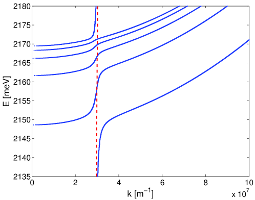
Figure 1: The polariton dispersion for a Cu₂O crystal, calculated by eq. (29), taking into account the 5 lowest excitonic states.

In the above dispersion relation only $P$ excitons are considered. The relation will much more complicated when excitons with higher angular momentu number will be included, for example $F$ or $H$ excitons.

V Anisotropy effects

The main difference between the effective hole and electron masses in Cu₂O is the high anisotropy observed for the hole masses while, as expected by symmetry, the electron value remains practically the same for all directions. The anisotropy in the hole effective masses is evidenced by their very different components in the [100], [110], and [111] directions (see, for example, Refs. Ching , Ruiz ). As was shown by Dasbach et al. Dasbach (see also Froelich ), the total exciton mass in the $[0,0,1]$ direction equals $3\leavevmode\nobreak\ m_{0}$, whereas the value in the $[1,1,0]$ direction is equal 0.66 (for example, Kazimierczuk ) or 0.5587 (Thewes ), see Table 1. The effective mass anisotropy plays an important role in the description of the optical properties of excitons. In the RDMA the anisotropy paramer $\alpha$ is defined, $\alpha=\mu_{\parallel}/\mu_{z}$, $\mu_{\parallel}=\mu[110]$ and $\mu_{z}$ being the electron-hole reduced masses in the respective directions. This parameter is then used in modified expressions for the excitonic eigenfunctions and eigenvalues. Instead of (15) we will use

$$R_{n\ell}(r)=C_{\ell}\left(2\lambda r\right)^{\ell}M\left(\ell+1-\frac{\eta_{\ell m}}{\lambda},2\ell+2,2\lambda r\right)\exp\left(-\lambda r\right),$$ (30)

with $\lambda=\sqrt{-E}$, $C_{\lambda}$ is the normalization factor, and

$$\eta_{\ell m}(\alpha)=\int\limits_{0}^{2\pi}{\rm d}\phi\int\limits_{0}^{\pi}\frac{|Y_{\ell m}|^{2}\sin\theta\,{\rm d}\theta}{\sqrt{\sin^{2}\theta+\alpha\cos^{2}\theta}}.$$ (31)

Bound states appear when the index $(\ell+1-\eta_{\ell m}/\lambda)$ attains zero or a negative integer, so that the discrete eigenvalues are given by RivistaGC , BCT95a :

$$E_{n\ell m}=-\frac{\eta^{2}_{\ell m}(\alpha)R^{*}}{n^{2}},\quad n=1,2,\ldots,\quad\ell=0,1,2,\ldots,n-1,\quad m=0,1,2,\ldots,\ell.$$ (32)

For the lowest eigenvalues we can use another expressions

$$E_{n\ell}=-A_{n\ell}^{2}R^{*},$$ (33)

with

$$A_{10} = \frac{2}{1+\sqrt{\alpha}},$$

$$A_{20} = \frac{2(1+2\sqrt{\alpha})}{3(1+\sqrt{\alpha})^{2}},$$ (34)

$$A_{30} = \frac{1}{15}\biggl{\{}\biggl{[}\frac{2}{1+\sqrt{\alpha}}$$

$$\times\left(\frac{\sqrt{\alpha}}{1+\sqrt{\alpha}}+2\frac{\sqrt{\alpha}}{(1+\sqrt{\alpha})^{2}}+\sqrt{\alpha}+3\right)\biggr{]}\biggr{\}}$$

etc., see Ref. BCT95a . The above formulas can explain the huge, as compared to the Rydberg energy, excitonic binding energy, for which we obtained the values 108.95 meV (105.32 meV), depending on the parametrs used, see Table 1. This values show the property of the observed exciton binding energy in Cu₂O, which is greater than the corresponding Rydberg energy (see, for example, Kavoulakis and, more recently, Frazer ). We can also calculate the $P$ and $F$ excitons resonances, using the values of the parameters $\eta_{10}$ and $\eta_{30}$. The results show that the $F$ exciton resonances are shifted to the higer energy, compared to the $P$ excitons (see Table 1), as was described in Ref. Thewes . Using the above results we can extend the expressions for the susceptibility, including the effects of $F$ excitons

$$\chi = \epsilon_{b}\sum\limits_{n=2}^{N}\frac{f_{n1}\Delta^{(2)}_{LT}/R^{*}}{\left(E_{Tn10}-E-{\rm i}{\mit\Gamma}\right)/R^{*}+(\mu_{\parallel}/M)(ka^{*})^{2}}$$ (35)

$$+\epsilon_{b}\sum\limits_{n=4}^{N}\frac{f_{n3}\Delta^{(2)}_{LT}/R^{*}}{\left(E_{Tn30}-E-{\rm i}{\mit\Gamma}\right)/R^{*}+(\mu_{\parallel}/M)(ka^{*})^{2}},$$

where the excitonic resonances are given at the energies

$$E_{Tn10} = -\frac{\eta_{10}^{2}}{n^{2}}R^{*},\quad n=2,3,\ldots,\qquad E_{Tn30}=-\frac{\eta_{30}}{n^{2}}R^{*},\quad n=4,5,\ldots$$ (36)

and

$$f_{n3}=\frac{(n^{2}-9)(n^{2}-4)(n^{2}-1)}{n^{9}}\cdot f,$$ (37)

where we set all remaining constants, including the unknown dipole matrix element $M_{03}$ as the factor $f$, which can be obtained, for example, by fitting the experimental spectra. In particular, the resonances for the $n=4$ state will be observed at the energies $E_{T410}=E_{g}-E_{410}=2158.6\leavevmode\nobreak\ \hbox{meV}$ ($P$ exciton) and $E_{T430}=E_{g}-E_{430}=2160\leavevmode\nobreak\ \hbox{meV}$ ($F$ exciton). This splitting is qualitatively in agreement with the observation by Thewes et al Thewes . The differences can be explained by the fact, that in Ref. Thewes another set of parameters (Rydberg energy, effective masses) was used, as can be seen in Table 1. Using the data of Ref. Thewes we obtain practically the same values for the excitonic resonances.

VI Green’s function method

The constitutive equation (2) is a nonhomogeneous differential equation, which can be solved by using the appropriate Green’s function. For bulk crystals, assuming the harmonic time-space dependence and only one valence$\to$conduction band transition, the Green function of the l.h.s. operator in (2) satisfies the equation

$$\left(E_{g}-\hbar\omega-{\rm i}{\mit\Gamma}+\frac{\hbar^{2}k^{2}}{2M}-\frac{\hbar^{2}}{2\mu}\hbox{\boldmath$\nabla$}^{2}-\frac{e^{2}}{4\pi\epsilon_{0}\epsilon_{b}r}\right)G\left({\bf r},{\bf r}^{\prime}\right)=\delta\left({\bf r}-{\bf r}^{\prime}\right).$$ (38)

Using the expansion

$$\delta\left({\bf r}-{\bf r}^{\prime}\right)=\frac{\delta\left(r-r^{\prime}\right)}{r^{2}}\sum\limits_{\ell=0}^{\infty}\sum\limits_{m=-\ell}^{\ell}Y^{*}_{\ell m}\left(\theta^{\prime},\phi^{\prime}\right)Y_{\ell m}(\theta,\phi),$$ (39)

where $Y_{\ell m}(\theta,\phi)$ are spherical harmonics, we look for the Green function in the form

$$G\left({\bf r},{\bf r}^{\prime}\right)=\sum\limits_{\ell=0}^{\infty}\sum\limits_{m=-\ell}^{\ell}Y^{*}_{\ell m}(\theta^{\prime},\phi^{\prime})Y_{\ell m}(\theta,\phi)g_{\ell m}(r,r^{\prime}).$$ (40)

Functions $g_{\ell m}$ satisfy the equations

$$\left(\frac{{\rm d}^{2}}{{\rm d}r^{2}}+\frac{2}{r}\frac{{\rm d}}{{\rm d}r}+\frac{2}{r}-\frac{\ell(\ell+1)}{r^{2}}-\kappa^{2}\right)g_{\ell m}=-\frac{2\mu}{\hbar^{2}a^{*}}\frac{\delta\left(r-r^{\prime}\right)}{r^{2}},$$ (41)

where $r$ is scaled in the excitonic Bohr radii (25), and

$$\kappa^{2}=\frac{2\mu}{\hbar^{2}}a^{*2}\left(E_{g}-\hbar\omega-{\rm i}{\mit\Gamma}\right)+\frac{\mu}{M}\left(ka^{*}\right)^{2}.$$ (42)

The solution of (41) is given in the form (for example, StB87 )

$$g_{\ell m}\left(r,r^{\prime}\right)=C\left(4\kappa^{2}rr^{\prime}\right)^{\ell}e^{-\kappa\left(r+r^{\prime}\right)}M\left(a_{\ell},b_{\ell},2\kappa r^{<}\right)U\left(a_{\ell},b_{\ell},2\kappa r^{>}\right),$$ (43)

where $r^{<}=$ min $(r,r^{\prime})$, $r^{>}$= max $(r,r^{\prime})$,

$$C = \frac{2\mu}{\hbar^{2}a^{*}}\frac{2\kappa\Gamma\left(a_{\ell}\right)}{\Gamma\left(b_{\ell}\right)},\qquad a_{\ell}=\ell+1-\frac{1}{\kappa},\qquad b_{\ell}=2\ell+2,$$ (44)

$M(a,b,c)$, $U(a,b,c)$ are $Kummer$ functions (confluent hypergeometric functions) in the notation of Abramowitz et al. Abramowitz , $Y_{\ell m}$ are spherical harmonics, $\Gamma(z)$ is the Euler Gamma-function, $a^{*}$ is the effective excitonic Bohr radius (25). Having the Green function, we calculate the coherent amplitudes

$$Y({\bf R},{\bf r})={\bf E}({\bf R})\int{\rm d}^{3}{r}^{\prime}{\bf M}({\bf r}^{\prime})G({\bf r},{\bf r}^{\prime}),$$ (45)

and thus the excitonic polarization from eq. (7)

$${\bf P}({\bf R})=\,2\int\int{\rm d}^{3}r{\rm d}^{3}r^{\prime}{\bf M}({\bf r})G({\bf r},{\bf r}^{\prime}){\bf M}({\bf r}^{\prime})\cdot{\bf E}({\bf R}).$$ (46)

The linear dielectric susceptibility tensor

$$\epsilon_{0}\underline{\underline{\chi}}(\omega,k)=2\int\int{\rm d}^{3}r{\rm d}^{3}r^{\prime}{\bf M}({\bf r})G({\bf r},{\bf r}^{\prime}){\bf M}({\bf r}^{\prime})$$ (47)

relates the electric field vector ${\bf E}$ to the polarization vector ${\bf P}$, and specific polarization components can be considered. From the above Green function expressions (45), (46) and (47) can be computed once an appropriate expression for ${\bf M}({\bf r})$ is considered.

Below the gap the imaginary part of the susceptibility $\chi(\omega,k)$ shows maxima in correspondence to the excitonic energy resonances. They are obtained from the singularities in the Green functions $g_{\ell m}$ and for $k=0,\Gamma=0$ are given by:

$$E_{Tn} = E_{g}+E_{n},$$

$$E_{n} = -\frac{R^{*}}{n^{2}},\qquad n=1,2,\ldots.$$ (48)

To simplify the calculations, we will use the transition dipole intensity in the form StB87

$$\textbf{M}(\textbf{r})=\textbf{M}_{10}\frac{\textbf{r}}{r_{0}^{3}}\delta(r-r_{0}),$$ (49)

and compute the susceptibility tensor element $\chi_{zz}$

$$\chi_{zz}(\omega,k) = \frac{2}{\epsilon_{0}}\int\int{\rm d}^{3}r{\rm d}^{3}r^{\prime}M_{z}({\bf r})G({\bf r},{\bf r}^{\prime})M_{z}({\bf r}^{\prime})$$

$$= \frac{2}{\epsilon_{0}}\int\int{\rm d}^{3}r{\rm d}^{3}r^{\prime}M_{z}({\bf r})\sum\limits_{\ell=0}^{\infty}\sum\limits_{m=-\ell}^{\ell}Y^{*}_{\ell m}(\theta^{\prime},\phi^{\prime})Y_{\ell m}(\theta,\phi)g_{\ell m}(r,r^{\prime})M_{z}({\bf r}^{\prime})$$

$$= \frac{4\pi^{2}}{3}\cdot\frac{2\mu}{\hbar^{2}}\epsilon_{b}\frac{2M_{10}^{2}}{\epsilon_{0}\epsilon_{b}\pi a^{*}}\cdot g_{10}(r_{0},r_{0})=\frac{4\pi^{2}}{3}\cdot\epsilon_{b}\frac{\Delta_{LT}}{R^{*}}g_{10}(r_{0},r_{0}),$$

with

$$g_{10}(r_{0},r_{0}) = \frac{\kappa\Gamma\left(a_{1}\right)}{3}\left(4\kappa^{2}r_{0}^{2}\right)e^{-2\kappa r_{0}}M\left(a_{1},4,2\kappa r_{0}\right)U\left(a_{1},4,2\kappa r_{0}\right),$$ (51)

$$a_{1}=2-\frac{1}{\kappa},\qquad b_{1}=4,$$

where $r_{0}$ is expressed in the units of $a^{*}$, and (42) is used in the form

$$\kappa^{2}=\frac{E_{g}-\hbar\omega-{\rm i}{\mit\Gamma}}{R^{*}}+\frac{\mu}{M}\left(ka^{*}\right)^{2}.$$ (52)

In a similar way one can calculate contributions of higher order excitonic states (F,H…) Having the susceptibility tensor elements obtained in terms of the Green function, we can alternatively compute the bulk absorption (in the limit $k\to 0$) and the polariton dispersion.

VII Results of specific calculations

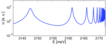
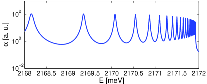
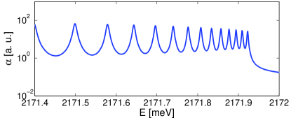
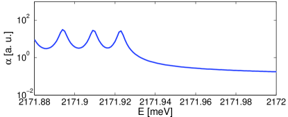
Figure 2: The bulk absorption of a Cu₂O crystal calculated by eq. (53) for four energy intervals below the fundamental gap. The logarithmic scale is applied.

We performed calculations for the Cu₂O crystal having in mind the experiments by Kazimierczuk et al. Kazimierczuk . The parameters used in calculations are collected in Table 1, where the Rydberg energy $95.74\leavevmode\nobreak\ \hbox{meV}$ and the effective excitonic Bohr radius $a^{*}=1.00\leavevmode\nobreak\ \hbox{nm}$ result from 18 and 25. First we calculated the polariton dispersion relation, shown in Fig. 1. We observe a multiplicity of values of the wave vectors, which means a multiplicity of polariton waves, much greater than those observed in other semiconductors as, for example, GaAs. This fact should certainly be regarded by computing the optical functions such as, for example, reflectivity, where the polaritonic aspect is relevant. Than we computed the absorption, shown in Fig. 2. Since the absorption peaks decrease quite rapidly, we applied the logarithmic scale. When the excitonic contributions of $F$ and $H$ are included, we observe the occurrence of additional absorption peaks, as shown in Fig. 3.

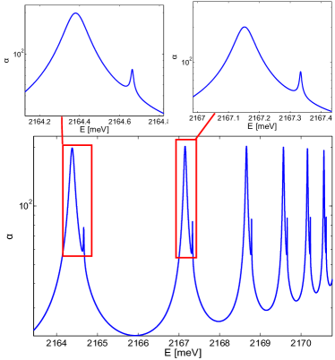
Figure 3: The absorption spectra including the effect of $P$ and $F$ excitons, calculated using the parameters from Ref. Thewes , see Table 1

By the relation (12) we can establish the dependence between the oscillator forces $f_{n1}$ and the corresponding state number $n$. The oscillator forces decrease with the number $n$, but the slope also depends on the coherence radius $r_{0}$. The general dependence is shown in Fig. 4, and in Fig. 5 we display the dependence on the coherence radius $r_{0}$. As it can be seen, the relation $f_{n}\propto n^{-3}$ is obtained only in the limit $r_{0}\to 0$. The best fit to the experimental spectra is obtained for $n^{-2.87}$, as shown in Fig. 4

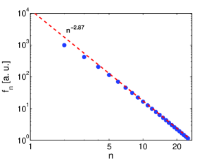
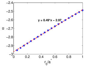
a) b)

Figure 4: a) The dependence of the oscillator forces $f_{n}$ on the state number $n$ with a linear fit added, b) The exponent $\alpha$ in the $n^{-\alpha}$ law as a function of the coherence radius $r_{0}$

In Fig. 5 we present the dependence of the absorption line shape on the magnitude of the coherence radius $r_{0}$.

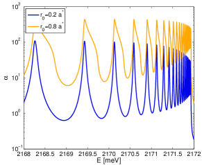
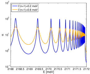
Figure 5: a) The dependence of the absoption line shape, calculated for two values of the coherence radius $r_{0}$, b) The dependence on the damping constant $\Gamma$

In the cases of semiconductors with large excitonic Bohr radii $a^{*}$ (large compared to the lattice constant as, for example, in GaAs) the coherence radius was taken as a small fraction of $a^{*}$. In the case of Cu₂O the Bohr radius is not very large (about twice) compared to the lattice constant. Therefore also $r_{0}$ cannot be very small. We can take, for example $r_{0}=0.5a^{*}$ but the exact value will be estimated by fitting the experimental spectra. As reported, for example, in Klingshirn , the longitudinal-transversal energy in Cu₂O is of the order of a few $\mu\hbox{eV}$. We put $\Delta_{LT}^{(2)}=10\mu\hbox{eV}$. Using eq. (29) and taking into account the lowest 25 excitonic states, we can determine the absorption coefficient from the relation

$$\alpha=10^{2}\frac{E\;[\hbox{meV}]}{1.976\leavevmode\nobreak\ \hbox{meV}\cdot\leavevmode\nobreak\ \hbox{cm}}\sqrt{\epsilon_{b}}\leavevmode\nobreak\ \hbox{Im}\leavevmode\nobreak\ \left[1+\sum\limits_{n=2}^{25}\frac{f_{n1}\Delta^{(2)}_{LT}}{E_{Tn10}-E-{\rm i}{\mit\Gamma}_{n1}}+\sum\limits_{n=4}^{25}\frac{f_{n3}\Delta^{(2)}_{LT}}{E_{Tn30}-E-{\rm i}{\mit\Gamma}_{n3}}+\ldots\right]^{1/2},$$ (53)

where only $m=0$ states where accounted for.

Recently, we became aware of a new experiment concerning absorption spectra which have taken into account the probability for absorbing photons from a laser as well as contributions relating to both coherent and incoherent parts of the spectrum of the excitons by Grünwald et al Grunwald .

VIII Final remarks

The main results of our paper can be summarized as follows. We have proposed a procedure based on the RDMA approach that allows to obtain analytical expressions for the optical functions of semiconductor crystals including high number Rydberg excitons, also for the case of indirect interband transitions. Our results have general character because arbitrary exciton angular momentum number is included. The effect of anisotropic dispersion and coherence of the electron and the hole with the radiation field is outlined. The theoretical findings are confirmed by numerical simulations. We have chosen the example of cuprous dioxide, inspired by the recent experiment by Kazimierczuk et al. Kazimierczuk . We have calculated the absorption spectrum, obtaining a very good agreement between the calculated and the experimentally observed spectra, including the splitting between the $P$ and $F$ excitons. We also obtained a good agreement with the experimental and theoretical results by Thewes et al. Thewes . We have derived the dipersion relation for polariton waves, which differs from the analogous relations for other semiconductors as, for example, GaAs. All these interesting features of excitons with high $n$ number which are examined and discussed on the basis on our theory might possibly provide deep insight into the nature of Rydberg excitons in solids and provoke their application to design all-optical flexible switchers and future implementation in quantum information processing.

Appendix A Appendix A. Derivation of the transition dipole density

In the real density matrix approach the coupling between the band edge and the radiation field is described by a smeared out transition dipole density $\textbf{M}(\textbf{r})$, r being the relative electron-hole distance. For the transition between the subbands $\nu_{1},\nu_{2}$ the definition is StB87 with the momentum operator $\textbf{p}_{\rho}(\textbf{k})$

$${\bf M}^{\nu_{1}\nu_{2}}({\bf r}) = :{\bf M}_{\rho}({\bf r})=\int\limits_{1.{\rm BZ}}{\rm d}^{3}k\tilde{M}_{\rho}({\bf k})e^{{\rm i}{\bf k}{\bf r}}$$ (54)

$$= \frac{1}{(2\pi)^{3}}\frac{{\rm i}e\hbar}{m_{0}}\int\limits_{1.{\rm BZ}}{\rm d}^{3}k\frac{{\bf p}_{\rho}e^{{\rm i}{\bf k}{\bf r}}}{E_{c}({\bf k})-E_{v\rho}({\bf k})}.$$

For allowed interband transitions we assume that $\textbf{p}(\textbf{k})\approx\textbf{p}(0)$ and that the interband energy is parabolic in relevant parts of k-space

$$E_{c}(\textbf{k})-E_{v}(\textbf{k})=E_{g}+\frac{\hbar^{2}k^{2}}{2\mu}.$$ (55)

Extending the integration to entire k-space one obtains (StB87 , CzB85 , see also Linear )

$$\textbf{M}(r)=\textbf{M}_{0}\frac{1}{4\pi r_{0}^{2}r}e^{-r/r_{0}},$$ (56)

with $r_{0}$ defined in eq. (20). In the case of the forbidden transtions $p(0)$ vanishes. The relevant transtion dipole density will be obtained from (54) by expansing the momentum operator in powers of k. To lowest nonvanishing order in k, we have $\textbf{p}(\textbf{k})\propto\textbf{k}$. Note that $k$ will arrive in the numerator of (54) after applying on both sides the operator $\nabla$. So we obtain

$$\textbf{M}(\textbf{r})\propto\,\hbox{\boldmath$\nabla$}\frac{e^{-r/r_{0}}}{r}=\frac{\textbf{r}}{r^{3}r_{0}}(r+r_{0})e^{-r/r_{0}}.$$ (57)

Requiring the normalization of the radial part we obtain the formula (19).

In general, the momentum operator $\textbf{p}_{cv}(\textbf{k})$ can be expanded in series of $k$:

$$\textbf{p}_{cv}(\textbf{k})=\textbf{p}_{cv}(0)+\textbf{k}\left[\hbox{\boldmath$\nabla$}_{k}\textbf{p}_{cv}(\textbf{k})\right]_{k=0}+....$$ (58)

Since we exploited the terms with $\textbf{p}_{cv}(0)$ and the term $\propto k$, the next terms will be proportional to $\textbf{p}(\textbf{k})\propto\textbf{k}(\textbf{k}\cdot\textbf{k})$, $\textbf{k}\cdot\textbf{k}$ means dyadic product. Performing, as above, the derivative operation with respect to $z$, (or $x,y$, respectively) on (56) and retaing the largest contributions, we obtain (for the sake of exemplification, we present the $z$-component)

$$M_{2} \propto \frac{3z^{2}-r^{2}}{r^{5}}e^{-r/r_{0}}=\sqrt{\frac{16\pi}{5}}\frac{Y_{20}}{r^{2}}e^{-r/r_{0}}=\sqrt{\frac{16\pi}{5}}r_{0}\frac{Y_{20}}{r^{2}}e^{-r/r_{0}},$$ (59)

$$M_{3z}\propto\frac{\partial^{3}}{\partial z^{3}} =\frac{3z(3r^{2}-5z^{2})}{r^{7}}e^{-r/r_{0}}=-12\sqrt{\frac{\pi}{7}}\frac{Y_{30}}{r^{4}}e^{-r/r_{0}},$$ (60)

$$M_{3x}\propto\frac{\partial^{3}}{\partial x^{3}} =\frac{3x(3r^{2}-5x^{2})}{r^{7}}e^{-r/r_{0}}$$

$$=\frac{1}{r^{4}}\left[\sqrt{\frac{3\pi}{7}}\left(Y_{31}-Y_{3-1}\right)-\sqrt{\frac{5\pi}{7}}\left(Y_{33}-Y_{3-3}\right)\right]e^{-r/r_{0}},$$

$$M_{3y}\propto\frac{\partial^{3}}{\partial y^{3}} =\frac{3y(3r^{2}-5y^{2})}{r^{7}}e^{-r/r_{0}}$$ (61)

$$=-{\rm i}\frac{1}{r^{4}}\left[\sqrt{\frac{3\pi}{7}}\left(Y_{31}+Y_{3-1}\right)-\sqrt{\frac{5\pi}{7}}\left(Y_{33}+Y_{3-3}\right)\right]e^{-r/r_{0}},$$

where $M_{2}$ corresponds to $D$ excitons, and $M_{3}$ to $F$ excitons, $M_{3}$ in unnormalized form.

Appendix B The calculation of the coefficients $b_{n1}$ and $b_{n3}$

First we calculate the coefficients $b_{n1}$ which define the susceptibility related to the $P$-excitons. Using the relations (22), (30), and (16), we obtain

$$C_{n1}^{2}\cdot\left(\frac{2}{na^{*}}\right)^{2} = \left(\frac{1}{3!}\right)^{2}\frac{(n+1)!}{2n(n-2)!}\left(\frac{2}{na^{*}}\right)^{3}\cdot\left(\frac{2}{na^{*}}\right)^{2}$$ (1)

$$= \frac{4}{9}\frac{n^{2}-1}{n^{5}}\frac{1}{a^{*5}}.$$

The above expression will be used in the calculation of the coefficients $b_{n1}$

$$b_{n1}=\frac{8\pi}{3}\left(\int\limits_{0}^{\infty}{\rm d}rr^{2}R_{n1}(r)M(r)\right)^{2}$$

$$=\frac{4\pi}{3}M_{10}^{2}C_{n1}^{2}\cdot\left(\frac{2}{na^{*}}\right)^{2}\left[\int\limits_{0}^{\infty}{\rm d}r\,r\,M\left(-n+2,4,\frac{2r}{a^{*}n}\right)\exp\left(-\frac{r}{na^{*}}\right)\frac{r+r_{0}}{r_{0}^{2}}e^{-r/r_{0}}\right]^{2}$$ (2)

$$=\frac{4\pi}{3r_{0}^{2}}M_{10}^{2}C_{n1}^{2}\cdot\left(\frac{2}{na^{*}}\right)^{2}\left\{\int\limits_{0}^{\infty}{\rm d}r\,r(r+r_{0})\,M\left(-n+2,4,\frac{2r}{a^{*}n}\right)\exp\left[-r\left(\frac{1}{na^{*}}+\frac{1}{r_{0}}\right)\right]\right\}^{2}.$$

Let us first calculate the integrals involving the confluent hypergeometric function

$$I=\int\limits_{0}^{\infty}{\rm d}r\,r(r+r_{0})\,M\left(-n+2,4,\frac{2r}{a^{*}n}\right)\exp\left[-r\left(\frac{1}{na^{*}}+\frac{1}{r_{0}}\right)\right]$$

$$=\int\limits_{0}^{\infty}{\rm d}r\,r^{2}\,M\left(-n+2,4,\frac{2r}{a^{*}n}\right)\exp\left[-r\left(\frac{1}{na^{*}}+\frac{1}{r_{0}}\right)\right]$$

$$+r_{0}\int\limits_{0}^{\infty}{\rm d}r\,r\,M\left(-n+2,4,\frac{2r}{a^{*}n}\right)\exp\left[-r\left(\frac{1}{na^{*}}+\frac{1}{r_{0}}\right)\right].$$

The above integrals can be expressed in terms of the hypergeometric function:

$$J_{\alpha\gamma}^{\nu}=\int\limits_{0}^{\infty}\;e^{-\lambda z}z^{\nu}M(\alpha,\gamma,kz)\,{\rm d}z=\Gamma(\nu+1)\lambda^{-\nu-1}F\left(\alpha,\nu+1,\gamma,\frac{k}{\lambda}\right),$$ (3)

$F(\alpha,\beta,\gamma,z)$ being the hypergeometric series

$$F(\alpha,\beta,\gamma,z)=1+\frac{\alpha\beta}{\gamma}\,\frac{z}{1!}+\frac{\alpha(\alpha+1)\beta(\beta+1)}{\gamma(\gamma+1)}\,\frac{z^{2}}{2!}+\ldots.$$ (4)

In the first approximation, assuming that $r_{0}\ll na^{*}$, which is certainly correct for large values of $n$, we have

$$I \approx 2\left(\frac{na^{*}r_{0}}{r_{0}+na^{*}}\right)^{3}+r_{0}\left(\frac{na^{*}r_{0}}{r_{0}+na^{*}}\right)^{2}=\left(\frac{na^{*}r_{0}}{r_{0}+na^{*}}\right)^{2}\left[2\frac{na^{*}r_{0}}{r_{0}+na^{*}}+r_{0}\right]$$

$$=r_{0}(3na^{*}+r_{0})\frac{(na^{*}r_{0})^{2}}{(r_{0}+na^{*})^{3}}$$

Thus

$$b_{n1}=\frac{4}{9}\frac{n^{2}-1}{n^{5}}\frac{1}{a^{*5}}\frac{4\pi}{3r_{0}^{4}}M_{10}^{2}\left[3\left(\frac{na^{*}r_{0}}{r_{0}+na^{*}}\right)^{3}\right]^{2}$$

$$=M_{10}^{2}\frac{n^{2}-1}{n^{5}}\frac{16\pi}{3}\left(\frac{a^{*}}{r_{0}}\right)^{4}\frac{1}{a^{*3}}\left(\frac{nr_{0}}{r_{0}+na^{*}}\right)^{6}.$$ (5)

For the $F$ excitons, taking $\ell=3$, we have

$$b_{n3}=\frac{144\pi}{7}\left(\int\limits_{0}^{\infty}{\rm d}rr^{2}R_{n3}(r)M_{3}(r)\right)^{2}$$

$$=\frac{144\pi}{7}M_{30}^{2}C_{n3}^{2}\cdot\left(\frac{2}{na^{*}}\right)^{6}\left\{\int\limits_{0}^{\infty}{\rm d}r\,r\,M\left(-n+4,8,\frac{2r}{a^{*}n}\right)\exp\left[-r\left(\frac{1}{na^{*}}+\frac{1}{r_{0}}\right)\right]\right\}^{2}$$

$$=\frac{256\cdot 144\cdot\pi\,r_{0}^{2}}{7(7!)^{2}a^{*9}}M_{30}^{2}\frac{(n^{2}-9)(n^{2}-4)(n^{2}-1)}{n^{9}}.$$ (6)

Roughly speaking, the oscillator strengths related to $F$ excitons also scale as $n^{-3}$, but are of order in magnitudes smaller than those of $P$ excitons, due to the factor $(7!)^{2}$ in denominator. In addition, the factor $(n^{2}-9)(n^{2}-4)(n^{2}-1)/{n^{9}}$ is smaller than $1/n^{3}$ as we can see, for example, for $n=4$ (0.0156 compared to $4.8\cdot 10^{-3}$). The same holds for the next odd $\ell$ value (5), where the factor $(11!)^{2}$ arrives in the denominator of the oscillator strength.

Appendix C Estimation of the coherence radius and the transition dipole matrix elements $M_{0}$

The formula (27) allows to estimate the matrix element $M_{10}$. Since $k=0$ at a longitudinal frequency $\omega_{L}$, taking from the r.h.s. the main contribution at $n=2$, we have

$$\epsilon_{0}\epsilon_{b}\Delta_{LT}^{(2)} = 2b_{21},$$ (7)

$$\Delta_{LT}^{(2)} = \hbar\omega_{L2}-\hbar\omega_{T2},$$ (8)

$$\Delta_{LT}^{(2)} = \frac{\pi}{\epsilon_{0}\epsilon_{b}a^{*3}}M_{10}^{2}\left(\frac{a^{*}}{r_{0}}\right)^{4}\left(\frac{2r_{0}}{r_{0}+2a^{*}}\right)^{6},$$ (9)

$$= R^{*}\cdot 2\frac{2\mu}{\hbar^{2}}\frac{M_{01}^{2}}{\pi\epsilon_{0}\epsilon_{b}a^{*}}f(r_{0},a^{*}),$$

with

$$f(r_{0},a^{*})=\frac{\pi^{2}}{2}\left(\frac{a^{*}}{r_{0}}\right)^{4}\left(\frac{2r_{0}}{r_{0}+2a^{*}}\right)^{6},$$ (10)

and with regard to the relation $2\mu/\hbar^{2}=1/R^{*}a^{*2}$. Higher order coefficients $b_{n1}$ can be expressed in terms of $b_{21}$

$${b_{n1}}=\frac{32(n^{2}-1)}{3n^{5}}\left[\frac{nr_{0}(r_{0}+2a^{*})}{2r_{0}(r_{0}+na^{*})}\right]^{6}{b_{2}}=\frac{16(n^{2}-1)}{3n^{5}}\left[\frac{nr_{0}(r_{0}+2a^{*})}{2r_{0}(r_{0}+na^{*})}\right]^{6}\epsilon_{0}\epsilon_{b}\Delta_{LT}^{(2)}=\frac{1}{2}f_{n1}\epsilon_{0}\epsilon_{b}\Delta^{(2)}_{LT},$$ (11)

with

$$f_{n1}=\frac{32(n^{2}-1)}{3n^{5}}\left[\frac{nr_{0}(r_{0}+2a^{*})}{2r_{0}(r_{0}+na^{*})}\right]^{6}.$$ (12)

The higher order longitudinal-transversal energies $\Delta_{LT}^{(n)}=\hbar\omega_{Ln}-\hbar\omega_{Tn}$ are related to the coefficients $b_{n1}$ by

$$2b_{n1}=\epsilon_{0}\epsilon_{b}\Delta_{LT}^{(n)}.$$ (13)

When $r_{0}\ll a^{*}$, (11) becomes

$$b_{n1}=\frac{32}{3}\,\frac{n^{2}-1}{n^{5}}\,b_{21},$$ (14)

or, in terms of $\Delta_{LT}^{(2)}$,

$$b_{n1}=\frac{16}{3}\,\epsilon_{0}\epsilon_{b}\frac{n^{2}-1}{n^{5}}\Delta_{LT}^{(2)},\qquad n=3,4,\ldots.$$ (15)

In the above equations and definitions, two parameters are used: the transition dipole matrix element $M_{01}$ and the coherence radius $r_{0}$. As it follows from eq. (9)

$$\frac{\Delta_{LT}^{(2)}}{R^{*}} = 2\frac{2\mu}{\hbar^{2}}\frac{M_{01}^{2}}{\pi\epsilon_{0}\epsilon_{b}a^{*}}f(r_{0},a^{*})=2\frac{M_{01}^{2}}{\epsilon_{0}\epsilon_{b}\pi R^{*}a^{*3}}f(r_{0},a^{*}),$$ (16)

the longitudinal-transversal splitting energy and the coherence radius are not independent quantities. Take, for example, the value of the transition dipole matrix element given in Ref. Mysyrowicz for the $1s\to 2p$ transition, in our notation $M_{0}=4.6\leavevmode\nobreak\ e\AA=1.08\cdot 10^{-28}\leavevmode\nobreak\ \hbox{C m}$. Using this value and other parameters for Cu₂O we obtain

$$\frac{\Delta_{LT}^{(2)}}{R^{*}}=4.55f(r_{0},a^{*}),$$ (17)

which means that a value of $\Delta_{LT}^{(2)}$ the order of 1 meV will be obtained for a small (compared to $a^{*}$) value of $r_{0}$. Thus the situation is the following: either we know the exact value of the LT-splitting energy (as is the case, for example, for GaAs), and the coherence radius can be estimated, or we consider $\Delta_{LT}$ and $r_{0}$ as two unknown quantities. Then we need two equations for establish them. Such equations can be obtained, for example, from the behavior of the dielectric function (here in scalar notation) $\epsilon(\omega)$,

$$\frac{c^{2}k^{2}}{\omega^{2}} = \epsilon(\omega,k)=\epsilon_{b}+\chi(\omega,k),$$ (18)

from which we obtain two equations

$$0 = \epsilon_{b}+\chi(\omega_{L},0),$$ (19)

$$\epsilon_{\infty} = \epsilon_{b}+\chi(\omega_{g},0),$$ (20)

($\epsilon_{\infty}=6.5$ for Cu₂O). From the above relations, which, in turn, also depend on the number of states taken into account, the relation between $r_{0}$ and $\Delta_{LT}$ can be obtained.

References

• (1) T. F. Gallagher, Rydberg Atoms, Cambridge Monographs on Atomic, Molecular and Chemical Physics (Cambridge University Press, Cambridge, 2005).
• (2) M. Weidemüller, Nature Physics 5, 91 (2009).
• (3) M. Saffman, T. G. Walker, and K. Molmer, Rev. Mod. Phys. 82, 2313 (2010).
• (4) H. Kübler, J. P. Shaffer, T. Baluktsian, R. Löw, and T. Pfau, Nature Photonic 4, 112, (2010).
• (5) B.T.H. Vercoe, S. Brattke, M. Weidinger, and H. Walther, Nature 403, 743 (2000).
• (6) S. Höfling and A. Kavokin, Nature 514, 313 (2014).
• (7) T. Kazimierczuk, D. Fröhlich, S. Scheel, H. Stolz, and M. Bayer, Nature 514, 344 (2014).
• (8) H. Friedrich and D. Wintgen, Phys. Rep. 183, 37, (1989).
• (9) H. Stolz, R. Schwartz, F. Kiesiling, S. Som, M. Kaupsch, S. Sobkowiak, D. Semkat, N. Naka, T. Koch, and H. Fehske, New J. Phys. 14, 105007 (2012).
• (10) A. Stahl and I. Balslev, Electrodynamics of the Semiconductor Band Edge (Springer-Verlag, Berlin-Heidelberg-New York, 1987).
• (11) G. Czajkowski, F. Bassani, and A. Tredicucci, Phys. Rev. B 54, 2035 (1996).
• (12) J. Thewes, J. Heckötter, T. Kazimierczuk, M. A$\beta$mann, D. Fröhlich, M. Bayer, M. A. Semina, and M. M. Glazov, Phys. Rev. Lett. 115, 027402 (2015), see also http://link.aps.org/ supplemental/10.1103/PhysRevLett.115.027402.
• (13) H. G. L. Tizei, Y. Ch. Lin, M. Mukai, H. Sawada, A.-Y. Lu, L. J. Li, K. Kimoto, and K. Suenaga, Phys Rev. Lett. 114, 107601 (2015).
• (14) G. Czajkowski and W. Chmara, Nuov. Cimento D 9, 1187 (1987).
• (15) J. L. Birman, Electrodynamics and Nonlocal Optical Effects mediated by Excitonic Polaritons, in Excitons, Modern Problems in Condensed Matter Sciences, edited by E. I. Rashba and M. G. Sturge, Vol.2 (North-Holland, Amsterdam, 1982), p. 27.
• (16) S. I. Pekar, Crystal Optics and Additional Light Waves (Benjamin-Cummings, Menlo Park, 1983).
• (17) V. M. Agranovich and V. L. Ginzburg, Crystal Optics with spatial Dispersion and Excitons (Springer Verlag, Berlin, 1984).
• (18) A. D’Andrea and R. Del Sole, Phys. Rev. B 32, 2337 (1985).
• (19) K. Cho, J. Phys. Soc. Japan 55, 4113 (1986).
• (20) A. D’Andrea and R. Del Sole, Phys. Rev. B 38, 1197 (1988).
• (21) G. Czajkowski, F. Bassani, and L. Silvestri, Rivista del Nuovo Cimento 26, 1-150 (2003).
• (22) V. M. Agranovich, Excitations in Organic Solids (Oxford University Press, Oxford, 2009).
• (23) W. Y. Ching, Yong-Nian Xu, and K. W. Wong, Phys. Rev. B 40, 7684 (1989).
• (24) E. Ruiz, S. Alvarez, P. Alemany, and R. A. Evarestov, Phys. Rev. B 56, 7190 (1997).
• (25) G. Dasbach, D. Frölich, H. Stolz, R. Klieber, D. Suter, and M. Bayer, Phys. Stat. Sol. C 2, 886 (2005).
• (26) D. Frölich, J. Brandt, Ch. Sundfort, and M. Bayer, Phys. Rev. B 84, 193205 (2011).
• (27) G. M. Kavoulakis, Y. -Ch. Chang, and G. Baym, Phys. Rev. B 55, 7593 (1997).
• (28) L. Frazer, K. B. Chang, K. R. Poeppelmeier, and J. B. Ketterson, Phys. Rev. B 89, 245203 (2014).
• (29) C. Klingshirn, Semiconductor Optics, 2nd ed., (Springer Verlag, Berlin Heidelberg New York, 2005).
• (30) F. Bassani, G. Czajkowski, and A. Tredicucci, Z. Phys. B 98, 39 (1995).
• (31) M. Abramowitz and I. Stegun, Handbook of Mathematical Functions (Dover Publications, New York, 1965).
• (32) P. Grünwald, M. Aßmann, D. Fröhlich, M. Bayer, H. Stolz, and S. Scheel, arXiv:1511.07742v1 [cond-mat.mes-hall] (2015).
• (33) T. Tayagaki, A. Mysyrowicz, and M. Kuwata-Gonokami, arXiv:cond-mat/0502584v3[cond-mat.mtrl-sci] 3 Mar 2005.
• (34) G. Czajkowski and I. Balslev, Phys. Stat. Sol B 130, 655 (1985).
• (35) G. Czajkowski, Linear optical properties of semiconductor nanostructures (UTP University Press, Bydgoszcz, 2006, ISBN 83-89334-78-X, in Polish).