Universal behavior of crystalline membranes: crumpling transition and Poisson ratio of the flat phase

Abstract

We revisit the universal behavior of crystalline membranes at and below the crumpling transition, which pertains to the mechanical properties of important soft and hard matter materials, such as the cytoskeleton of red blood cells or graphene. Specifically, we perform large-scale Monte Carlo simulations of a triangulated two-dimensional phantom network which is freely fluctuating in three-dimensional space. We obtain a continuous crumpling transition characterized by critical exponents which we estimate accurately through the use of finite-size techniques. By controlling the scaling corrections, we additionally compute with high accuracy the asymptotic value of the Poisson ratio in the flat phase, thus characterizing the auxetic properties of this class of systems. We obtain agreement with the value which is universally expected for polymerized membranes with a fixed connectivity.

I Introduction

Crystalline or polymerized membranes (CM) constitute a natural two-dimensional generalization of the simple idea behind one-dimensional polymeric chains. Namely, a two-dimensional arrangement of monomers, which are connected by rigid bonds that never break Bowick01 . CM are expected to provide good approximations to the mechanical properties of a number of interesting two-dimensional material systems. Among others Bowick96 , they account for the thermal fluctuations of the cytoskeleton of red blood cells Schmidt93 ; Boal12 and provide an accurate first step to describe the unique mechanical properties of graphene Katsnelson12 ; Katsnelson2013 . Such mechanical features include e.g. the existence of intrinsic, thermally-induced ripples in the graphene sheet Fasolino07 ; Braghin10 , which can strongly influence the electronic and magnetic properties Katsnelson12 of this important two-dimensional material.

In thermal equilibrium, the phase diagram of crystalline membranes possesses a number of remarkable properties Nelsonetal04 . Thus, in contrast with polymers in solution DesCloizeaux90 , CM are flat (albeit rough) at low temperatures, namely, the local normal directions at different points of the membrane have a well-defined average orientation. Nevertheless, there is a phase transition to a crumpled morphology at a finite value of temperature, above which the local normal directions are disordered. For the case of phantom CM, namely, in the absence of self-avoidance, both, theoretical and numerical studies confirm this behavior Bowick01 ; Nelson04 ; Gompper04 , which also differs from what is found for fluid membranes Leibler04 . For self-avoiding membranes in physical dimensions, namely, a two-dimensional network fluctuating in three-dimensional space, there is no crumpling transition Bowick01_b . Rather, a unique phase exists for all temperatures which is flat, with similar characteristics to the low-temperature phase of phantom membranes.

The flat phase of crystalline membranes also hosts another remarkable property Falcioni97 , namely, auxetic behavior, which is signaled by a negative Poisson ratio $\sigma$ Greaves11 . This property implies that the membrane expands transversely when stretched longitudinally, contrary with experience with most common elastic materials. Auxetic materials are expected to have good mechanical properties Greaves11 , such as high energy absorption and fracture resistance; see in particular Grima15 for a recent study of the potential of graphene from this point of view, as assessed by Molecular Dynamics simulations. Moreover, the conjectured negative value of $\sigma$ seems to be independent of the occurrence of self-avoidance constraints, $\sigma=-1/3$ —as obtained within the so-called self-consistent screening approximation (SCSA) Doussal92 — having been put as characteristic of a unique universality class for fixed-connectivity membranes Bowick01_c .

In spite of these interesting properties of the flat phase of crystalline membranes, they remain to be fully understood. For instance, the nature of the crumpling transition is still a subject of debate. While the computational and analytical works quoted above mostly suggested that it is a continuous transition, more recent results suggest, rather, a first order transition. Numerical results supporting the latter conclusion have been obtained for a number of CM-related models in e.g. Refs. Kownacki02 (with a truncated Lennard-Jones potential) and Koibuchi04 ; Koibuchi05 ; Koibuchi14 (spherical topology). Results from non-perturbative renormalization group (RG) calculations are in agreement with these Essafi14 . Nevertheless, analogous RG studies Kownacki09 ; Braghin10 ; Hasselmann11 seem to still favor a continuous, or perhaps weak first order, crumpling transition.

In this paper we revisit Monte Carlo simulations of a discrete model of two-dimensional phantom membranes fluctuating in three dimensions Bowick96 . By implementing our simulations in graphics processor units (GPU), we are able to reach large system sizes; we further implement an enhanced statistical analysis of data. Our results favor the view of the crumpling transition as a continuous one and feature clear-cut convergence to the expected $-1/3$ value of the Poisson ratio characterizing the universal auxetic properties of the flat phase Doussal92 .

The paper is organized as follows. In Sec. II we recall the basics of the continuum description of phantom membranes, together with a detailed connection to the discrete model to be simulated numerically. Section III details the observables to be evaluated and their finite-size analysis. Our simulation and statistical analysis methods are described in Sec. IV, after which numerical results are presented in Sec. V. We discuss our main results and summarize our conclusions in Sec. VI. Three appendices are provided for details on some elasticity equations, renormalization group (RG) estimates for the correction-to-scaling exponent, and on the practical implementation of our simulation code in GPUs.

II Model

II.1 Continuum description

For the sake of later reference, we briefly recall here the basics of the Landau description of (phantom) polymerized membranes in physical dimensions. Thus, a two-dimensional membrane fluctuating in three-dimensional space can be described geometrically as a vector field $\vec{r}(x^{1},x^{2})\in\mathbb{R}^{3}$, with $\mathitbf{x}=(x^{1},x^{2})\in\mathbb{R}^{2}$. The tangent vectors are $\vec{t}_{\alpha}=\partial_{\alpha}\vec{r}$, where, as for all additional Greek indices in this work, $\alpha=1,2$. These vectors allow us to define the metric tensor in the usual way David04 ,

$$g_{\alpha\beta}\equiv\partial_{\alpha}\vec{r}\cdot\partial_{\beta}\vec{r}\,,$$ (1)

so that $d^{2}s=d^{2}x\sqrt{g}$.

The most general form of the Landau free energy can be written using general principles Paczuski88 ; Nelson04 , namely: locality and translational invariance (implying dependence only on the local values of the tangent vectors $\vec{t}_{\alpha}$ and their derivatives), rotational symmetry in $\mathbb{R}^{3}$ (implying dependence on scalar products of the tangent vectors and their derivatives, and on even powers of these) and translational and rotational invariance in $\mathbb{R}^{2}$. Thus, one can write Paczuski88 ; Nelson04

$$F[\vec{t}_{\alpha}(\mathitbf{x}),T] = \int d^{2}s\left[\frac{t}{2}(\vec{t}_{\alpha})^{2}+u(\vec{t}_{\alpha}\vec{t}_{\beta})^{2}+v(\vec{t}_{\alpha}\vec{t}^{\alpha})^{2}\right.$$ (2)

$$+ \left.\frac{\kappa}{2}(\partial_{\alpha}\vec{t}_{\alpha})^{2}\right],$$

where self-avoidance is neglected Bowick01 .

One can parameterize the three-dimensional coordinates $\vec{r}$ of points on a flat membrane taking as a reference the base plane, namely, the plane determined by the average position of all the atoms. Denoting the equilibrium position on this plane by $\mathitbf{x}$, and in-plane and perpendicular fluctuations by $\mathitbf{u}$ and $h$, respectively, we have

$$\vec{r}(\mathitbf{x})=(\mathitbf{x}+\mathitbf{u(x)},h(\mathitbf{x})),$$ (3)

where $\langle(\mathitbf{u(\mathitbf{x})},h(\mathitbf{x}))\rangle=0$.

Moreover, on a flat membrane the strain tensor can be written as Nelson04

$$u_{\alpha\beta}=\frac{1}{2}\left(\partial_{\alpha}\vec{r}\cdot\partial_{\beta}\vec{r}-\delta_{\alpha\beta}\right)=\frac{1}{2}\left(g_{\alpha\beta}-\delta_{\alpha\beta}\right)\,.$$ (4)

Taking into account the in-plane ($\mathitbf{u}$) and out-plane ($h$) displacements, and neglecting quadratic terms in $u_{\alpha}$, we can write

$$u_{\alpha\beta}=\frac{1}{2}\left(\partial_{\alpha}u_{\beta}+\partial_{\beta}u_{\alpha}+\partial_{\alpha}h\partial_{\beta}h\right).$$ (5)

The so-called elastic part of the Landau free energy (2), namely,

$$F_{E}[\vec{t}_{\alpha}(\mathitbf{x}),T]=\int d^{2}s\left[\frac{t}{2}(\vec{t}_{\alpha})^{2}+u(\vec{t}_{\alpha}\vec{t}_{\beta})^{2}+v(\vec{t}_{\alpha}\vec{t}^{\alpha})^{2}\right],$$ (6)

can now be written as

$$F_{E}(\vec{r})=\int d^{2}xf_{E}(\vec{r})=\int d^{2}x\left[\mu u_{\alpha\beta}u^{\alpha\beta}+\frac{\lambda}{2}(u_{\alpha}^{\alpha})^{2}\right]\,,$$ (7)

where $\lambda$ and $\mu$ are the Lamé coefficients metric . The remaining part of the Landau free energy, namely,

$$F_{C}[\vec{t}_{\alpha}(\mathitbf{x}),T]=\int d^{2}s\left[\frac{\kappa}{2}(\partial_{\alpha}\vec{t}_{\alpha})^{2}\right]$$ (8)

is a curvature contribution that can be written as

$$F_{C}[\vec{t}_{\alpha}(\mathitbf{x}),T]=2\kappa\int d^{2}xK_{\alpha}^{\beta}K^{\alpha}_{\beta},$$ (9)

where indeed $K_{\alpha}^{\beta}$ is the extrinsic curvature extrinsic .

II.2 Discrete model

Figure 1: (color online) Lattice that has been employed in this work, for $L=6$, in which a four-color partition is illustrated. Points with the same color can be updated simultaneously. This partition has been used to speed up, in a highly parallel way, our numerical simulations using GPU processors.

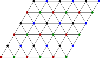
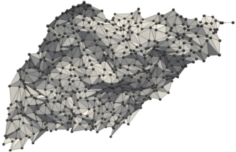
We define our computational model on an $N=L\times L$ two-dimensional triangular lattice like the one shown in see Fig. 1, embedded in three-dimensional space, see Fig. 2. The position of the points is thus labeled by a three-dimensional vector $\vec{r}$. We also define triangular plaquettes with associated normal vectors denoted as $\vec{n}$. In general, we will denote points using the indices $i$, $j$, $k$, etc. and plaquettes using $a$, $b$, $c$, etc.

Figure 2: (color online) Sample membrane configuration at $\kappa=2$ in the flat phase, for $L=24$.

The Hamiltonian we study is

$${\cal H}={\cal H}_{E}+\kappa{\cal H}_{C},$$ (10)

which includes an elastic part, ${\cal H}_{E}$, given by

$${\cal H}_{E}=\frac{1}{2}\sum_{<ij>}|\vec{r}_{i}-\vec{r}_{j}|^{2},$$ (11)

and a curvature contribution, ${\cal H}_{C}$, which reads

$${\cal H}_{C}=\frac{1}{2}\sum_{<ab>}|\vec{n}_{a}-\vec{n}_{b}|^{2}.$$ (12)

As usual, $<ij>$ denotes nearest-neighbor points, while $<ab>$ denotes nearest-neighbor plaquettes.

Within a mean-field approach, it is possible to show Seung88 ; Bowick96 ; Monroy13 that the above Hamiltonians retrieve the corresponding contributions to the Landau free energy in the continuum limit, namely,

$${\cal H}_{E}\to\int d^{2}s\left(\frac{1}{2}u_{\alpha}^{\alpha}u_{\beta}^{\beta}+u_{\alpha\beta}u^{\alpha\beta}\right),$$ (13)

$${\cal H}_{C}\to\int d^{2}sK_{\alpha}^{\beta}K^{\alpha}_{\beta}.$$ (14)

III Observables and the Finite Size Scaling Method

The specific heat can be computed as Harnish1991

$$C_{V}=\frac{\kappa^{2}}{N}\left(\langle E_{C}^{2}\rangle-\langle E_{C}\rangle^{2}\right)\,,$$ (15)

where

$$E_{C}=\sum_{<ab>}\vec{n}_{a}\cdot\vec{n}_{b}\,,$$ (16)

is the curvature energy. The behavior of the specific heat near the crumpling transition that takes place at $\kappa=\kappa_{c}$ is characterized as,

$$C_{V}\sim|\kappa-\kappa_{c}|^{-\alpha}\,.$$ (17)

The correlation length is defined using the correlation among the normals of the system,

$$\langle\vec{n}(x)\cdot\vec{n}(0)\rangle\propto e^{-|x|/\xi}\,,$$ (18)

the scaling law for $\xi$ being

$$\xi(\kappa)\sim|\kappa-\kappa_{c}|^{-\nu}\,.$$ (19)

Right at the critical point, the maximum of the specific heat scales as

$$C_{\mathrm{max}}\propto C_{a}+BL^{\alpha/\nu}\,.$$ (20)

where $C_{a}$ describes the contribution from the analytical part of the free energy.

We can further describe the space configuration of the membrane by considering the gyration radius for the distribution of surface nodes, which is defined as

$$R^{2}_{g}=\frac{1}{3N}\langle\sum_{i}\vec{R}_{i}\cdot\vec{R}_{i}\rangle\,,$$ (21)

where $\vec{R}_{i}\equiv\vec{r}_{i}-\vec{r}_{\text{CM}}$, with $\vec{r}_{\text{CM}}$ the position of the center of mass of the surface. In addition, linear response theory allows us to compute its $\kappa$-derivative,

$$\frac{dR^{2}_{g}}{d\kappa}=\langle E_{C}R^{2}_{g}\rangle-\langle E_{C}\rangle\langle R^{2}_{g}\rangle\equiv\langle E_{C}R^{2}_{g}\rangle_{c}.$$ (22)

Neglecting scaling corrections, the gyration radius scales with the system size as

$$R_{g}\sim L^{\nu_{F}}f(L^{1/\nu}(\kappa-\kappa_{c})),$$ (23)

which defines the Flory exponent $\nu_{F}$. This exponent is related with the Hausdorff dimension, $d_{H}$, of the membrane by means of

$$\nu_{F}=\frac{2}{d_{H}}.$$ (24)

Near the crumpling transition, one finds $d_{H}=-4/\eta$, where $\eta$ is the anomalous dimension of the $\vec{r}$-field Espriu96 . In the flat phase one has $d_{H}=2$ and $\nu_{F}=1$, while the high temperature rough phase features $\nu_{F}=0$ and $d_{H}=\infty$, which is linked with a logarithmic divergence of the gyration radius, $R_{G}^{2}\sim\log L$. Therefore, the $\kappa$-derivative of the gyration radius diverges at the critical point $\kappa=\kappa_{c}$ as

$$\frac{dR^{2}_{g}}{d\kappa}\propto L^{2\nu_{F}+1/\nu}\,,$$ (25)

an equation that will allow us to compute numerically the Flory exponent. Note that, using the SCSA approximation, it has been found that $\nu=0.73$ and hence $d_{H}=2.74$ Doussal92 .

Finally we can estimate the Poisson ratio via (see Appendix A)

$$\sigma=\frac{K-\mu}{K+\mu}=-\frac{\langle g_{11}g_{22}\rangle_{c}}{\langle g_{22}^{2}\rangle_{c}}=-\frac{\langle g_{11}g_{22}\rangle_{c}}{\langle g_{11}^{2}\rangle_{c}}\,,$$ (26)

where $g$ is the induced metric that can be estimated using the vector which connects nearest neighbor points, as described in Appendix A. Note that we have assumed isotropy in the last two terms in Eq. (26), specifically, $\langle g_{11}^{2}\rangle_{c}=\langle g_{22}^{2}\rangle_{c}$.

IV Numerical Simulations

We have performed Monte Carlo (MC) simulations on triangular lattices of different sizes using a standard Metropolis algorithm. We have performed simulations for several months both on CPUs (Intel Core I7-3770) and GPUs (NVIDIA Tesla C2070). While the MC sweep of each site on the lattice on CPUs is entirely sequential, in GPUs we can parallelize the simulation using a kind of checkerboard scheme with four colours, see Fig. 1 and Appendix C for details. We have obtained a gain factor around 5x simulating on GPUs.

We have simulated lattice sizes in the $16\leq L\leq 128$ range, using free-boundary conditions. The thermalization protocol has been as follow: 1) we have always started from a flat configuration, 2) we have discarded the first $10^{6}$ Metropolis sweeps, and 3) we have analyzed the remainder of the run using a logarithmic binning check of several non local observables in the most challenging simulations, i.e., for $\kappa\simeq\kappa_{c}$.

After thermalization, we have saved $10^{5}$ configurations with at least $10^{4}$ Metropolis sweeps between each pair of saved configurations. Via the computation of the integrated autocorrelation times Amit2005 we have checked that all our measures are fully independent. To estimate the error bars of our observables we always used a jackknife method with 20 bins.

For each lattice size, we have considered several values of $\kappa$ around $\kappa_{c}$, as well as $\kappa$ values well inside the flat phase, in general we have simulated the range $0.75\leq\kappa\leq 3.0$.

V Numerical Results

V.1 Crumpling Transition

Figure 3: (color online) Behavior of the specific heat as a function of temperature for all simulated lattice sizes. The solid black curves provide the least-squares fit of the points near the maximum to a quadratic form as described in the text. We have used pentagons ($L=16$), rhombs ($L=24$), inverted triangles ($L=32$), triangles ($L=48$), circles ($L=64$), squares ($L=96$) and crosses ($L=128$) to mark the points in the figure.

Figure 4: (color online) Behavior of the $\kappa$-derivative of the squared gyration radius as a function of temperature for all simulated lattice sizes. The solid black curves provide the least-squares fit of the points near the maximum to a quadratic form as described in the text. We have used pentagons ($L=16$), rhombs ($L=24$), inverted triangles ($L=32$), triangles ($L=48$), circles ($L=64$), squares ($L=96$) and crosses ($L=128$) to mark the points in the figure.

Figure 5: (color online) Scaling of the maximum of the specific heat (pentagons) as a function of the size of the system. The solid line is a fit to Eq. (20).

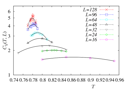
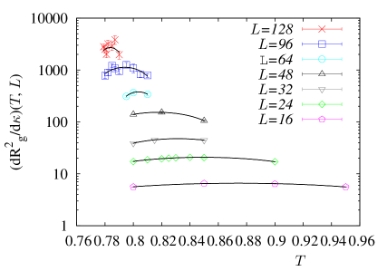
In Figs. 3 and 4 we show the behaviors of the specific heat and $dR^{2}_{g}/d\kappa$ as functions of $\kappa$. The onset of a critical behavior is clear in both figures. To compute the maximum of both observables, we have fitted each curve near its maximum using least-squares (for $L<96$ we have also used the spectral density method). Monte Carlo has been performed on the raw data in order to compute the error bars, both in the value of the maximum as well as in its position.

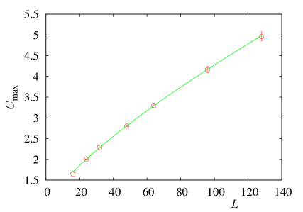
In order to characterize the critical properties (order of the phase transition, critical exponents, etc.), we first monitor the behavior of the maximum of the specific heat, see Fig. 5. By using data with $L>16$, we find a clear divergence of this maximum following a power-law with a background term, as stated in Eq. (20) above, with $\alpha/\nu=0.756(40)$ ($\chi^{2}/\mathrm{d.o.f.}=0.78/3$, where d.o.f. means the number of degree of freedom of the fit). This $\alpha/\nu=0.756(40)$ value is definitively different from 2, characteristic of a strong first-order phase transition, or even from 1 which would indicate a weak first-order transition Fernandez92 . By using hyper-scaling in two dimensions [$\alpha=2(1-\nu)$], we can compute simultaneously both $\alpha$ and $\nu$, to get

$$\nu=0.73(1)\,\,,\,\,\alpha=0.55(2)\,.$$ (27)

Figure 6: (color online) Position of the maximum of the specific heat (lower data, see legend, pentagons) and of the maximum of $dR^{2}_{g}/d\kappa$ (inverted triangles) as a function of $L^{-1/\nu}$. In this plot we have employed $1/\nu=1/0.73$, as obtained from the fit of the peak of the specific heat. We have used the position of the specific heat maximum to obtain $\kappa_{c}$. Finally, we have fitted $dR^{2}_{g}/d\kappa$ by imposing the previous obtained values of $\nu$ and $\kappa$, hence there is a single free parameter in the fit. The solid (specific heat) and dashed (gyraton radius) lines are “linear” fits in this scale. Notice that the gyration radius presents stronger scaling corrections than the specific heat.

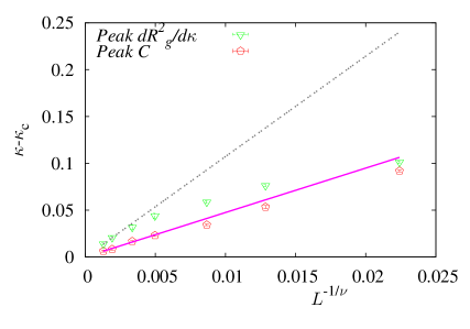
Using the $\nu$-exponent obtained from the scaling of the maximum (see Fig. 6) of the specific heat, we can study the $\kappa$-position of this maximum, denoted as $\kappa(L)$. This $\kappa(L)$ follows the standard scaling equation (neglecting scaling corrections),

$$\kappa(L)=\kappa_{c}+AL^{-1/\nu}\,,$$ (28)

where $\kappa_{c}$ is the infinite volume critical coupling. By using the $\nu$ value from Eq. (27), we obtain

$$\kappa_{c}=0.773(1)\,,$$ (29)

where we have taken into account $L>32$ data only ($\chi^{2}/\mathrm{d.o.f.}=2.016/2$). We have been unable to compute the correction-to-scaling exponent of the crumpling transition.

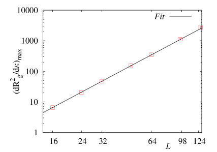
We can redo the previous analysis on the derivate of the squared gyration radius (Fig. 6). The scaling of the maximum of $dR^{2}_{g}/d\kappa$ (see Fig. 7) provides us with the following combination of exponents, see Eq.(25),

$$2\nu_{F}+\frac{1}{\nu}=2.86(1),$$ (30)

with $\chi^{2}/\text{d.o.f.}=3.5/5$ ($L\geq 16$). Using again the $\nu$ value obtained from the analysis of the specific heat, we can obtain the Flory exponent, equivalently the Hausdorff dimension, of the surface at criticality, taking into account the error bars in our value of $\nu$:

$$\nu_{F}=0.74(1)\,\,,\,\,d_{H}=2.70(2)\,.$$ (31)

Figure 7: (color online) Scaling of the maximum of the $\kappa$-derivative (squares) of the squared gyration radius, $dR^{2}_{g}/d\kappa$, as a function of system size. The solid line is a fit to Eq. (25).

V.2 Poisson ratio in the flat phase

We next study the low-temperature (equivalently, large $\kappa$) flat phase of phantom crystalline membranes in more detail (see Ref. Troster13 for a detailed computation of the $\eta$-exponent). In this ordered phase, long-range order exists in the orientation of surface normals. Moreover, this phase is known to host auxetic behavior Bowick01 .

As mentioned in the introduction, auxetic materials have acquired a huge importance, both from the fundamental and from the technological points of views Greaves11 . The flat phase of CM membranes unambiguously shows a negative value of the Poisson ratio. However, a detailed study of the scaling corrections in this phase is still lacking, while numerical data should be extrapolates to infinite volume in order to perform a proper comparison with analytical results. In particular, the value $\sigma=-1/3$, obtained by the SCSA approximation Doussal92 , has been hypothesized to characterize a unique universality class for fixed-connectivity membranes Bowick01_c .

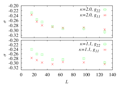
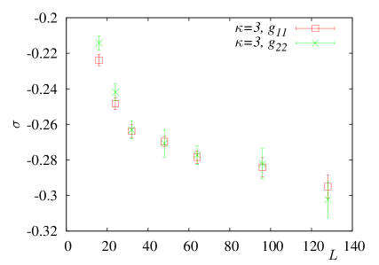
We have first explicitly checked the isotropy of finite-size membranes in the flat phase. To do this, we have monitored the two different definitions of the Poisson ratio, namely, Eq. (26) using $g_{11}$ in the denominator, or else using $g_{22}$. Figs. 8 and 9 show the values of $\sigma$ as obtained using these two definitions, for three different conditions on $\kappa$ within the flat phase. For $\kappa=1.1$, which is near the crumpling transition, we have found lack of isotropy for almost all simulated lattice sizes, see Fig. 8. However, we can safely assume isotropy for $\kappa=2$ and $L>32$, and for $L>16$ if $\kappa=3.0$, see Figs. 8 and 9. In the following, we will only consider $\kappa=2,3$, and values of the lattice size for which isotropy holds.

Figure 8: (color online) Comparison between the computation of the Poisson ratio using $g_{11}$ or $g_{22}$ as the denominator in Eq. (26), see legend. Notice the strongly anisotropic behavior of the Poisson ratio for $\kappa=1.1$ (lower panel). For $\kappa=2$ (upper panel), isotropy holds for $L>32$.

Figure 9: (color online) Comparison between the computation of the Poisson ratio using $g_{11}$ (squares) or $g_{22}$ (crosses) as the denominator in Eq. (26) for $\kappa=3$, see legend. Isotropy holds for $L\geq 24$.

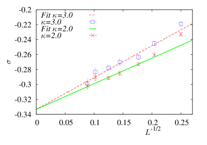
In order to extract the asymptotic value of the Poisson ratio, we will use the standard scaling form,

$$\sigma(L)=\sigma_{\infty}+\frac{A}{L^{\omega}},$$ (32)

where $\omega$ corresponds to the leading correction-to-scaling exponent in the flat phase. We recall that the analytical prediction is $\sigma_{\infty}=-1/3$ Doussal92 .

We have obtained very good fits for both values of $\kappa=2,3$. Specifically, for $\kappa=2$ we obtain $\sigma_{\infty}=-0.30(1)$ and $\omega=1.3(9)$ ($\chi^{2}/\mathrm{d.o.f.}=2.30/2$), while $\kappa=3$ leads to $\sigma_{\infty}=-0.31(2)$ and $\omega=0.76(47)$ ($\chi^{2}/\mathrm{d.o.f.}=4.8/3$). In both cases the asymptotic value of the Poisson ratio is fully compatible with the analytical prediction. We can try to improve our analysis by fixing $\sigma_{\infty}=-1/3$. For $\kappa=2.0$ this leads to $\omega=0.44(6)$ ($\chi^{2}/\mathrm{d.o.f.}=4.8/3$), while for $\kappa=3$ we obtain $\omega=0.46(5)$ ($\chi^{2}/\mathrm{d.o.f.}=4.4/4$).

Finally, we have tried a simultaneous fit of the $\kappa=2$ and 3 data, i.e., a fit in which we assume that the values of $\sigma_{\infty}$ and $c$ in Eq. (32) are the same for both $\kappa$, and in which we allow for different values of $A$. The result of this joint fit is $\sigma_{\infty}=-0.317(12)$ and $\omega=0.63(20)$ ($\chi^{2}/\mathrm{d.o.f.}=8.4/7$). Further, a joint fit in which we fix $\sigma_{\infty}=-1/3$ leads to $\omega=0.46(2)$ ($\chi^{2}/\mathrm{d.o.f.}=9.6/8$). Figure 10 displays the linear dependence of the Poisson ratio with $1/\sqrt{L}$.

Figure 10: (color online) Finite-size effects in the Poisson ratio for $\kappa=2$ and 3. We have fixed the scaling correction exponent to 1/2 and the asymptotic value to the analytical value, $\sigma_{\infty}=-1/3$. We have used crosses and solid line fit ($\kappa=2$) and squares and dashed line fit ($\kappa=2$).

VI Discussion and conclusions

We have studied in detail important universal properties associated with the flat phase of crystalline membranes, specifically the nature of the crumpling transition and auxetics. With respect to the former, we have found clear signatures for a second order phase transition. The values we obtain for the critical exponents rule out completely an interpretation in terms of a strong, or even a weak, first order phase transition, as had been proposed in the literature recently.

In order to asses the crumpling transition as a continuous one, we have studied the critical behavior of the specific heat and of the $\kappa$-derivative of the gyration radius. In our numerical analysis, we have employed realistic boundary conditions for the membrane (free boundary conditions). We have also avoided restricting the computation of our observables to an inner region far from the boundary, as done elsewhere, see e.g. Ref. Bowick96 .

The values we obtain for the critical exponents [$\alpha=0.55(2)$, $\nu=0.73(1)$, $\nu_{F}=0.74(1)$, and $d_{H}=2.70(2)$] compare very well with previous results. For the specific-heat exponent, we can mention $\alpha=0.5(1)$ Bowick96 , 0.58(10) Wheater96 , and 0.44(5) Renken90 . For the correlation length exponent, $\nu=0.72(2)$ Renken90 , 0.68(10) Wheater96 , and 0.85(14) Espriu96 . Regarding the value of the critical coupling, we can quote $\kappa_{c}=0.814(2)$ Wheater96 , to be compared with our result, $\kappa_{c}=0.773(1)$. Finally, the value for the Flory exponent or, equivalently, for the Haussdorf dimension, should be compared with the analytical results $\nu_{F}=0.73$, $d_{H}=2.73$ Doussal92 and those from numerical simulations, $\nu_{F}=0.71(3)$, $d_{H}=2.77(10)$ Espriu96 .

Regarding comparison with previous results, we believe that in many cases the error bars provided for the critical exponents reported in the literature have been clearly underestimated. We have computed the error bars after a carefully study of the different integrated correlation times, having simulated among the largest available lattices. In spite of this, e.g. the value of the critical coupling reported by some previous numerical works is incompatible with our numerical result, which points out a potential inadequacy of the corresponding statistical analysis of numerical data. For instance, $\kappa_{c}\simeq 0.82$ Espriu96 and 0.814(2) Wheater96 are previous determinations of the critical coupling which are 18 standard deviations from the value we obtain.

Beyond the nature and critical exponents of the crumpling transition, we have further studied the value of the Poisson ration in the flat phase as a further universal property of CM. This seems particularly interesting in view of the huge scientific and technological importance that auxetic materials are displaying in recent years Greaves11 .

In particular, we have simulated three different values of $\kappa$ above the crumpling transition and in the flat phase, in order to compute the asymptotic value of the Poisson ratio. We have discarded the smallest $\kappa$ value due to the huge anisotropies that occur for almost all simulated lattice sizes. By using the largest two values of $\kappa$, we have found a very precise infinite-volume extrapolation for the Poisson ratio which is in very good agreement with the analytical value $\sigma_{\infty}=-1/3$ computed in Ref. Doussal92 . In order to reach this conclusion, control of scaling corrections has been required. We have specifically found numerically that the scaling corrections behave as $1/\sqrt{L}$. Our extrapolated value for $\sigma$ is compatible with previous numerical work Bowick96 ; Falcioni97 ; Bowick01_c which postulates such a value as characteristic of a universality class of membranes with fixed connectivity.

In principle, graphene is believed to provide a conspicuous experimental realization of crystalline membranes. In this context, e.g. the model provided by Eq. (2) is being intensively employed on a phenomenological basis as a prototype to describe the statistical-mechanical properties of this important material system Katsnelson12 ; Katsnelson2013 . Nevertheless, some of the behaviors of graphene like, for instance, the temperature dependence of the bending rigidity, seem to remain beyond this type of phenomenological approach Katsnelson12 ; Katsnelson2013 . The fact that the Poisson ratio of graphene is positive unless, e.g., temperature is sufficiently high Zakharchenko2009 or defects are introduced into the crystalline structure Grima15 , suggests that predicting realistic values of $\sigma$ also remains beyond current phenomenological models of graphene membranes. From the theoretical point of view, it will be interesting to identify which is the nature of the modifications to be made on generic models like Eq. (2) so that they can eventually improve upon this type of predictions.

VII Acknowledgments

This work was partially supported by Ministerio de Economía y Competitividad (Spain) through Grants No. FIS2012-38866-C05-01 and No. FIS2013-42840-P, by Junta de Extremadura (Spain) through Grant No. GRU10158 (partially funded by FEDER), and by European Union through Grant No. PIRSES-GA-2011-295302. We also made use of the computing facilities of Extremadura Research Centre for Advanced Technologies (CETA-CIEMAT), funded by the European Regional Development Fund (ERDF).

Appendix A Some elasticity equations

In this appendix we recall some standard elasticity equations and use them to obtain Eq. (26), which has been employed in this work to compute numerically the Poisson ratio.

The starting point is Eq. (7), considered as a Hamiltonian, see Ref. Lubensky88 ; Falcioni97 . This equation can be rewritten as

$${\cal H}_{E}(u_{\alpha,\beta}) = \int d^{2}x\left[\mu\left(u_{\alpha\beta}-\frac{1}{2}\delta_{\alpha\beta}\right)\left(u^{\alpha\beta}-\frac{1}{2}\delta^{\alpha\beta}\right)\right.$$ (33)

$$+ \left.\frac{1}{2}Ku_{\alpha}^{\alpha}u_{\beta}^{\beta}\right]\,,$$

where $K=\lambda+\mu$ is the compressibility modulus. From this equation we can compute the stress tensor, $\sigma_{\alpha\beta}$ stress

$$\sigma_{\alpha\beta}(\mathitbf{x}) = \langle\frac{\delta{\cal H}_{E}}{\delta{u^{\alpha\beta}}(\mathitbf{x})}\rangle=K\delta_{\alpha\beta}\langle u_{\gamma}^{\gamma}(\mathitbf{x})\rangle$$ (34)

$$+ 2\mu\left(\langle u_{\alpha\beta}(\mathitbf{x})\rangle-\frac{1}{2}\delta_{\alpha\beta}\langle u_{\gamma}^{\gamma}(\mathitbf{x})\rangle\right)\,.$$

Using that $\sigma_{\gamma}^{\gamma}=2K\langle u_{\gamma}^{\gamma}\rangle$, it is possible to invert the last equation, obtaining

$$\langle u_{\alpha\beta}(\mathitbf{x})\rangle=\frac{1}{4K}\delta_{\alpha\beta}\sigma_{\gamma}^{\gamma}(\mathitbf{x})+\frac{1}{2\mu}\left(\sigma_{\alpha\beta}(\mathitbf{x})-\frac{1}{2}\delta_{\alpha\beta}\sigma_{\gamma}^{\gamma}(\mathitbf{x})\right)\,.$$ (35)

The Poisson ratio can be written as Landau75

$$\sigma=-\frac{\langle u_{22}\rangle}{\langle u_{11}\rangle}=\frac{K-\mu}{K+\mu}\,,$$ (36)

where the directions $x^{1}$ and $x^{2}$ on the substrate (the $\mathitbf{x}$-plane) on which lives the flat surface are denoted by the indices 1 and 2, respectively.

Using the linear response theorem, we can write Falcioni97

$$\langle u_{\alpha\beta}(\mathitbf{x})u_{\gamma\delta}(\mathitbf{y})\rangle_{c}=\frac{\delta\langle u_{\alpha\beta}(\mathitbf{x})\rangle}{\delta\sigma^{\gamma\delta}(\mathitbf{y})}\,,$$ (37)

where $\langle(\cdot\cdot\cdot)\rangle_{c}$ denotes the connected average as elsewhere in this work. In addition, taking the derivative of Eq. (35), one can obtain

$$\frac{\delta\langle u_{\alpha\beta}(\mathitbf{x})\rangle}{\delta\sigma^{\gamma\delta}(\mathitbf{y})} = \left(-\frac{K-\mu}{4\mu K}\delta_{\alpha\beta}\delta_{\gamma\delta}\right.$$ (38)

$$+ \left.\frac{1}{4\mu}\left(\delta_{\alpha\gamma}\delta_{\beta\delta}+\delta_{\alpha\delta}\delta_{\beta\gamma}\right)\right)\delta(\mathitbf{x}-\mathitbf{y})\,.$$

Notice that, in a continuous system with a finite area, $\delta(\mathitbf{0})=1$ Lubensky2000 . Using the last two equations, we can write

$$\langle u_{11}(\mathitbf{x})u_{22}(\mathitbf{x})\rangle_{c}=\frac{K-\mu}{4\mu K}\,,$$ (39)

$$\langle u_{12}(\mathitbf{x})u_{12}(\mathitbf{x})\rangle_{c}=\frac{1}{4\mu}\,,$$ (40)

$$\langle u_{11}^{2}(\mathitbf{x})\rangle_{c}=\langle u_{22}^{2}(\mathitbf{x})\rangle_{c}=\frac{K+\mu}{4\mu K}\,.$$ (41)

Hence, we can finally write Eq. (36) as

$$\sigma=\frac{K-\mu}{K+\mu}=-\frac{\langle u_{11}u_{22}\rangle_{c}}{\langle u_{11}^{2}\rangle_{c}}=-\frac{\langle u_{11}u_{22}\rangle_{c}}{\langle u_{22}^{2}\rangle_{c}}\,,$$ (42)

which, when written in terms of the metric $g_{\alpha\beta}(\mathitbf{x})$, gives us Eq. (26) of the main text.

Note that we can compute the tangent vectors, $\partial_{i}\vec{r}$, as differences. Here, $i=1,2,3$ run on the three natural directions of the triangular lattice, which are not orthogonal, while in the definition of $\sigma$ we assume that the deformations are mutually orthogonal Landau75 . Hence, we have defined two orthogonal axes $\mathitbf{x}_{1}$ and $\mathitbf{x}_{2}$, taking $\mathitbf{x}_{1}=\mathitbf{e}_{1}$ and $\mathitbf{x}_{2}=(\mathitbf{e}_{2}+\mathitbf{e}_{3})/\sqrt{3}$, where $\mathitbf{e}_{1}$, $\mathitbf{e}_{2}$ and $\mathitbf{e}_{3}$ are the three natural unit vectors on the triangular lattice. Finally, we compute the induced metric, $g_{\alpha\beta}$, in this basis.

Appendix B RG computation of the correction-to-scaling exponent for the flat phase

We can obtain a prediction within the RG framework, for the value of the correction-to-scaling exponent for the flat phase. Following Refs. Lubensky88 and Bowick01 , within an $\epsilon$-expansion the renormalized (dimensionless) elastic constants, $\hat{\mu}$ and $\hat{\lambda}$, have the following $\beta$-functions (denoted as $\beta_{\hat{\mu}}$ and $\beta_{\hat{\lambda}}$):

$$\beta_{\hat{\lambda}} = \frac{d{\hat{\lambda}}}{d\log l}=-\epsilon{\hat{\mu}}+\frac{{\hat{\mu}}^{2}}{8\pi^{2}}\left(\frac{1}{3}d_{c}+20A\right)\,,$$ (43)

$$\beta_{\hat{\mu}} = \frac{d{\hat{\mu}}}{d\log l}=-\epsilon{\hat{\lambda}}+\frac{1}{8\pi^{2}}\left[\frac{1}{3}d_{c}{\hat{\mu}}^{2}\right.$$ (44)

$$+ \left.2(d_{c}+10A){\hat{\lambda}}{\hat{\mu}}+2d_{c}{\hat{\lambda}}^{2}\right]\,.$$

Here, $A=({\hat{\mu}}+{\hat{\lambda}})/(2{\hat{\mu}}+{\hat{\lambda}})$. In our present case, $\epsilon=2$ and $d_{c}=1$ Bowick01 . Eqs. (43)-(44) present four fixed points. Out of these, the physical behavior is controlled by the one characterized by ${\hat{\lambda}}=-4\epsilon/(24+d_{c})$ and ${\hat{\mu}}=12\epsilon/(24+d_{c})$.

In order to compute the correction-to-scaling exponent, we need to obtain the eigenvalues, denoted by $\lambda_{1}$ and $\lambda_{2}$, of these two couplings via the diagonalization of the Jacobian matrix of the $\beta$-functions Amit2005 . Note, both eigenvalues are expected to be negative, as the system lies on the critical surface. Indeed, the result is

$$\lambda_{1} = \frac{(65-125\pi^{2})\epsilon}{125\pi^{2}}\,,$$ (45)

$$\lambda_{2} = \frac{125(1-\pi^{2})\epsilon}{125\pi^{2}}\,.$$ (46)

Setting $\epsilon=2$, we obtain $\lambda_{1}\simeq-1.90$ and $\lambda_{2}\simeq-1.80$. Hence, $\omega\simeq-1.80$ at this perturbative order.

Finally we can compute the value of the Poisson ratio, by using that, at the physical fixed point, $\hat{\lambda}/\hat{\mu}=-1/3$, thus $\sigma=\hat{\lambda}/(\hat{\lambda}+2\hat{\mu})=-1/5$. Notice that both values for $\omega$ and $\sigma$ are far from the corresponding MC results. We can conclude that, due to the large value of $\epsilon$, it is very difficult to extract reliable predictions from the RG at this perturbative order.

Appendix C Implementation of the code in GPU

As widely acknowledged Wei2012 , pretty good gain factors can be obtained by using Graphic Processing Units (GPU). In our case, the gain was almost guaranteed, given that we use mostly floating point variables that can be updated in parallel following some kind of checkerboard algorithm. The gain factor depends strongly on the system size, but we obtain at least a factor of 5x.

The Compute Unified Device Architecture (CUDA) implementation of the Metropolis algorithm stores a single copy of the surface in the GPU memory. By operating only in the GPU memory, we reduce memory controller load and reduce the computation time required per iteration. The surface update kernel is executed sequentially over a quarter of the surface nodes and returns to CPU mode once all nodes have been processed, see Fig. 1.

The structure of the algorithm requires performing an atomic operation over a single variable to sum the total number of updated node positions. This is the hardest bottleneck in the algorithm.

Due to the parallel update structure, we need to generate a random seed for each node in the surface, as opposed to the CPU sequential version, in which a single seed is enough. The number of blocks and threads per block in the CUDA simulation is given by the surface size and the maximum number of GPU registers assigned to each thread. The limit in the number of registers that a kernel can use has a great impact on the overall performance.

References

- (1) M. J. Bowick and A. Travesset, Phys. Rep. 344, 255 (2001).
- (2) M. J. Bowick, S. Catterall, M. Falcioni, G. Thorleifsson and K. N. Anagnostopoulus, J. Phys. France 6, 1321 (1996).
- (3) C. F. Schmidt, K. Svoboda, N. Lei, I. B. Petsche, L. E. Berman, C. R. Safinya, and G. S. Grest, Science 259, 952 (1993).
- (4) D. Boal, Mechanics of the Cell, 2nd. edition (Cambridge University Press, Cambridge, UK, 2012).
- (5) M. I. Katsnelson, Graphene: carbon in two dimensions (Cambridge University Press, Cambridge, UK, 2012).
- (6) M. I. Katsnelson and A. Fasolino, Acc. Chem. Res. 46, 97 (2013).
- (7) A. Fasolino, J. H. Los, and M. I. Katsnelson, Nat. Mater. 6, 858 (2007).
- (8) F. L. Braghin and N. Hasselmann, Phys. Rev. B 82, 035407 (2010).
- (9) D. R. Nelson, S. Piran, and S. Weinberg, editors, Statistical Mechanics of Membranes and Surfaces, 2nd. edition, (World Scientific, Singapore, 2004).
- (10) J. des Cloizeaux and G. A. Jannink, Polymers in Solution, Their Modelling and Structure (Oxford University Press, Oxford, 1990).
- (11) D. R. Nelson, in Nelsonetal04 , pp 1 and 133.
- (12) G. Gompper and D. M. Kroll, in Nelsonetal04 , p 359.
- (13) S. Leibler, in Nelsonetal04 , p 49.
- (14) M. J. Bowick, A. Cacciuto, G. Thorleifsson, and A. Travesset, Eur. Phys. J. E 5, 149 (2001).
- (15) M. Falcioni, M. J. Bowick, E. Guitter, and G. Thorleifsson, Europhys. Lett. 38, 67 (1997).
- (16) G. N. Greaves, A. L. Greer, R. S. Lakes, and T. Rouxel, Nat. Mater. 10, 823 (2011).
- (17) J. N. Grima, S. Winczewski, L. Mizzi, M. C. Grech, R. Cauchi, R. Gatt, D. Attard, K. W. Wojciechowski, and J. Rybicki, Adv. Mater. 27, 1455 (2015).
- (18) P. Le Doussal and L. Radzihovsky, Phys. Rev. lett. 69, 1209 (1992).
- (19) M. Bowick, A. Cacciuto, G. Thorleifsson, and A. Travesset, Phys. Rev. Lett. 87, 148103 (2001).
- (20) J.-Ph. Kownacki and H. T. Diep, Phys. Rev. E 66, 066105 (2002).
- (21) H. Koibuchi, N. Kusano, A. Nidaira, K. Suzuki, and M. Yamada, Phys. Rev. E 69, 066139 (2004).
- (22) H. Koibuchi and T. Kuwahata, Phys. Rev. E 72, 026124 (2005).
- (23) H. Koibuchi and A. Shobukhov, Int. J. Mod. Phys. C 25 1450033 (2014).
- (24) K. Essafi, J.-P. Kownacki, and D. Mouhanna, Phys. Rev. E 89, 042101 (2014).
- (25) J.-P. Kownacki and D. Mouhanna, Phys. Rev. E 79 040101R (2009).
- (26) N. Hasselmann and F. L. Braghin, Phys. Rev. E 83, 031137 (2011).
- (27) F. David, in Nelsonetal04 , p 149.
- (28) M. Paczuski, M. Kardar, and D. R. Nelson, Phys. Rev. Lett. 60, 2638 (1988).
-
(29)
Notice that, using the flat membrane parameterization (Monge parameterization),
, the metric tensor can be evaluated as
Hence, to order , one can freely raise and lower incides. Moreover, . -
(30)
The extrinsic curvature matrix is defined in the usual way David04 : The
derivative of a tangent vector can be expressed in the (local) basis of the
membrane tangent vectors and normal vector (denoted as ) as
where are the Christoffel symbols (affine connection). - (31) H. S. Seung and D. R. Nelson, Phys. Rev. A 38, 1005 (1988).
- (32) P. Monroy, Transiciones de fase en membranas cristalinas, Masters thesis, Universidad de Extremadura (2013).
- (33) R. G. Harnish and J. F. Wheater, Nucl. Phys. B 350, 861 (1991).
- (34) D. Espriu and A. Travesset, Nucl. Phys. B 466, 514 (1996).
- (35) D. J. Amit and V. Martin-Mayor, Field Theory, the Renormalization Group, and Critical Phenomena: Graphs To Computers, 3rd. edition (World Scientific, Singapore, 2005).
- (36) L. A. Fernandez, M. P. Lombardo, J. J. Ruiz-Lorenzo, and A. Tarancon, Phys. Lett. B274, 485 (1992).
- (37) J. F. Wheater, Nucl. Phys. B 458, 671 (1996).
- (38) R. L. Renken and J. B. Kogut, Nucl. Phys. B 342, 753 (1990).
- (39) K. V. Zakharchenko, M. I. Katsnelson, and A. Fasolino, Phys. Rev. Lett. 102, 046808 (2009).
- (40) J. A. Aronovitz and T. C. Lubensky, Phys. Rev. Lett. 60, 2634 (1988).
(41)
One way to obtain this equation is to write a Schwinger-Dyson equation using the identity
where we have assumed that the fields vanish at the boundary of the functional integration. See, for instance, Refs. Landau75 ; Falcioni97 and Amit2005 . - (42) L. D. Landau and E. M. Lifshitz, Theory of Elasticity (Pergamon Press, Oxford 2008)
- (43) P. M. Chaikin and T. C. Lubensky, Principles of Condensed Matter Physics (Cambridge University Press, Cambridge, UK, 2000).
- (44) A. Tröster, Phys. Rev. B 87, 104112 (2013).
- (45) M. Weigel, J. Comput. Phys. 231, 3064 (2012).