Wilkinson’s Inertia-Revealing Factorization and Its Application to Sparse Matrices

Abstract

[Summary]We propose a new inertia-revealing factorization for sparse symmetric matrices. The factorization scheme and the method for extracting the inertia from it were proposed in the 1960s for dense, banded, or tridiagonal matrices, but they have been abandoned in favor of faster methods. We show that this scheme can be applied to any sparse symmetric matrix and that the fill in the factorization is bounded by the fill in the sparse $QR$ factorization of the same matrix (but is usually much smaller). We describe our serial proof-of-concept implementation, and present experimental results, studying the method’s numerical stability and performance.

, , and (2017), Wilkinson’s Inertia-Revealing Factorization and Its Application to Sparse Matrices, Numer Linear Algebra Appl, XXX.

1 Introduction

The inertia of a real symmetric matrix $A$ is a triplet of numbers that count how many of $A$’s eigenvalues are positive, negative or zero, respectively. The first two of these numbers are called the positive and negative indices of inertia, respectively, and the last one is the nullity of the matrix. The inertia is easy to obtain by computing all of the eigenvalues of $A$. However, even for moderately large sparse problems, computing all of the eigenvalues is either expensive or infeasible. Over the years, inertia algorithms have been developed that do not resort to computing the full spectrum. Such algorithms are the focus of this paper.

A fast inertia algorithm can facilitate a number of computational tasks. As a first example, consider an eigenvalue of $A$ that is isolated from the rest of the spectrum within a known interval $[x_{0},x_{1})$. Let us see how to compute the multiplicity of that eigenvalue by taking advantage of a fast inertia algorithm. The key is the property that the negative index of inertia of the matrix $A-xI$, where $x$ is real, is the number of eigenvalues of $A$ that lie to the left of $x$. To compute the multiplicity, we compute the negative indices of inertia of the matrices $A-x_{1}I$ and $A-x_{0}I$, and subtract the latter index from the former. This yields the number of eigenvalues that are to the left of $x_{1}$ but not to the left of $x_{0}$, which is exactly the multiplicity of the target eigenvalue.

The same idea works if we need to compute the aggregate multiplicity of all of the eigenvalues within a known interval. This is useful when we compute all of the eigenvalues within that interval using a Lanczos shift-and-invert eigensolver, and we wish to ascertain that no eigenvalues have been missed.[zhang07]

Another example is when we need to compute a histogram of the spectrum within an interval of interest. In this case, we divide the interval into subintervals and compute the number of eigenvalues within each subinterval using the above technique. Such a histogram is necessary when we wish to compute all of the eigenvalues within the interval of interest, and we need to partition the work evenly among multiple processors.[aktulga14] Here, each inertia computation is independent from the others, which makes this scheme suitable for parallel computation.

The final example is bisection. In bisection, we compute the eigenvalues of $A$ by using the negative index of inertia of $A-xI$ as a binary-search oracle for locating the eigenvalues by their ordinals (for an example, see Golub and Van Loan[golub13]*Sec 8.4.1).

To facilitate the above (and similar) tasks, we propose a new algorithm that computes the inertia of sparse symmetric matrices. Our new sparse inertia algorithm combines two old and obsolete algorithmic ideas into a useful and novel algorithm. One idea is an algorithm that was proposed by Wilkinson[wilkinson65]*p 236–240 for computing the inertia of dense, banded, or tridiagonal matrices. Wilkinson recommended the algorithm as the building block of a bisection eigensolver for tridiagonal matrices. Over the years, this algorithm was replaced by the use of $LDL^{T}$ factorizations of shifts of the matrix (and by other tridiagonal eigensolvers; see [demmel97, parlett98, stewart01]). The newer alternatives are more efficient and more stable; Wilkinson’s inertia idea appeared to be obsolete. The other idea is the row-by-row sparse $QR$ factorization by George and Heath.[george80] It was replaced by sparse multifrontal $QR$ factorizations[liu86] (for a recent implementation, see [davis11a]). We have discovered that George and Heath’s approach to sparse factorizations and its analysis can be applied to Wilkinson’s inertia algorithm. This discovery is what motivates the new algorithm.

Existing algorithms for computing the inertia of sparse matrices work by computing a so-called symmetric-indefinite factorization (see [duff83] for an early example). Such algorithms work well in practice, but they are heuristic in the sense that no guarantees can be made about the amount of work and memory that they require on any individual matrix. In contrast, on many important classes of matrices, the new algorithm provides an a priori bound on the fill that it generates and hence on its storage requirements and (indirectly) on its running time. A counterintuitive feature of the algorithm is that it computes a nonsymmetric factorization; we sacrifice symmetry, but we gain bounds on the fill.

Our implementation of the method is inspired by CSparse, Tim Davis’s concise sparse-matrix library.[davis06] We felt that it was premature to invest the kind of engineering effort that is required to produce production-quality sparse-matrix factorization software, and so we translated the method into code in a straightforward way, opting for simplicity whenever possible. This means that the resulting code is serial and does not provide optimal performance, but its performance is predictable and easy to understand to anyone who understands the basic algorithm.

The rest of the paper is organized as follows. We present the required background material in Section 2. Section 3 describes our sparse implementation and its effect on the sparsity pattern of the matrix. We analyze the numerical stability of the algorithm in Section 4, and present numerical experiments in Section 5. The performance of our implementation is studied experimentally in Section 6, followed by our conclusions from this research in Section 7.

2 Background

2.1 General-Purpose Eigensolvers

Eigenvalues of symmetric dense matrices are almost always computed using a two-step procedure.[golub13]*Sec 8 In the first step, we reduce the matrix to tridiagonal form using a sequence of orthogonal similarity transformations. This reduction has the form $Q^{T}AQ=T$, where $Q$ is orthogonal and $T$ is tridiagonal. The reduction preserves the spectrum of $A$ and allows us to compute $A$’s eigenvalues by applying a tridiagonal eigensolver to $T$; this is the second step.

The computational cost of reducing an $n$-by-$n$ matrix $A$ to $T$ is $\Theta(n^{3})$ arithmetic operations, and the cost of tridiagonal eigensolvers such as bisection, the implicit $QR$ method or the more recent MRRR algorithm[dhillon06] is $\Theta(n^{2})$. Because of the upfront investment in reducing the matrix to $T$, there is no advantage in computing a subset of the eigenvalues; the whole spectrum is produced at essentially the same cost. Eigenvectors can also be computed: this costs $\Theta(n^{2})$ for the eigenvectors of $T$ and $\Theta(n^{3})$ to transform them into eigenvectors of $A$ by reversing the effect of the orthogonal similarities.

2.2 Lanczos

The orthogonal-tridiagonalization approach is not suitable for sparse matrices because orthogonal similarity transformations fill the matrix with nonzeros, resulting in a computational cost of $\Theta(n^{3})$ even when $A$ is very sparse. The most widely applicable approach for sparse symmetric eigenproblems is the Lanczos iteration. Here we compute an orthogonal basis $Q$ of the Krylov subspace $K_{t}=\operatorname{span}(b,Ab,\dotsc,A^{t-1}b)$, where $t$ is the dimension of the subspace and $b$ is a nonzero starting vector, usually chosen at random. We then use $Q$ to orthogonally project $A$ along the Krylov subspace, producing a $t$-by-$t$ tridiagonal matrix $T$ whose eigenvalues serve as approximations to the eigenvalues of $A$. A popular implementation of this approach is the implicitly restarted Lanczos method, available in the ARPACK library.[calvetti94, lehoucq97]

Lanczos produces each column of $Q$ by multiplying $A$ with the previous column, and then orthogonalizing the resulting vector against the existing columns. The computational cost is $t-1$ matrix-vector products and $\Theta(t^{2}n)$ arithmetic operations for the orthogonalization operations. Typical sparse matrices can be of dimension $10^{6}$ or higher, and so letting $t$ approach $n$ or even $\sqrt{n}$ would make the computational cost prohibitive. For this reason, the number of iterative steps is usually chosen to be much smaller than $n$. Stopping after a small number of iterations means that only a few of $A$’s eigenvalues are well approximated, typically those at the edges of the spectrum.

When we wish to compute eigenvalues in the interior of the spectrum, we compute a triangular factorization of $A-\sigma I$, where $\sigma$ is the point of interest in the spectrum, and iterate with $\left(A-\sigma I\right)^{-1}$ instead of iterating with $A$. Under this transformation, every eigenvalue $\lambda$ of $A$ is mapped to an eigenvalue $(\lambda-\sigma)^{-1}$ in the transformed matrix’s spectrum. The eigenvalues that are closest to $\sigma$ in $A$’s spectrum map to the outermost eigenvalues of $(A-\sigma I)^{-1}$, which leads Lanczos to converge to those eigenvalues first. This is called shift-and-invert Lanczos.

The drawback of Lanczos is that it is hard to use as a black-box solver. Convergence depends on the structure of the spectrum, and there is no way to ascertain that all of the required eigenvalues have been obtained. Another difficulty stems from the fact that the projection of $K_{t}$ along any eigenspace of $A$ is one dimensional, and therefore Lanczos cannot determine the multiplicities of the eigenvalues of $A$. If we wish to determine multiplicities, we can use a variant called block Lanczos, but the costs rise with the dimension of the computed eigenspace, which limits the efficiency of this approach. Some of these deficiencies are addressed by algorithms popular in the electronic-structure calculations community, such as conjugate gradients and FEAST.[ovtchinnikov08, polizzi09]

2.3 Bisection

Bisection is a recursive algorithm that computes all of the eigenvalues that lie in a user-specified half-open interval $\left[x_{0},\;x_{1}\right)$. Since computing an interval that envelops the entire spectrum is relatively easy (e.g., using the bound $|\lambda|\leq\|A\|_{2}\leq\|A\|_{1}$; see [golub13]*Thm 7.2.1), the requirement for a user-provided interval does not limit the generality of the method. Bisection works by splitting the interval into two halves, counting the eigenvalues in each half, and continuing the search recursively in each half that contains eigenvalues. To count the eigenvalues in an interval $\left[x_{0},\;x_{1}\right)$, we determine the numbers $f(x_{0})$ and $f(x_{1})$ of eigenvalues that lie strictly to the left of $x_{0}$ and of $x_{1}$; the difference $f(x_{1})-f(x_{0})$ is the number of eigenvalues in the interval. The function $f(x)$ is evaluated by computing the negative index of inertia $\nu$ of $A-xI$,

$$f(x)=\nu(A-xI)\,.$$

The recursion stops when the length $x_{1}-x_{0}$ of the current interval falls below a user-specified tolerance threshold. At this point, the algorithm returns the midpoint of the interval as a representative of the eigenvalues within that interval. The midpoint is duplicated as many times as there are eigenvalues. (Duplication can represent either tight clusters of distinct eigenvalues or multiple eigenvalues).

A pseudocode of bisection is given in Algorithm 1. The code can be easily modified to compute only the eigenvalues inside a user-specified interval or a set of eigenvalues that are specified by their ordinals.

Algorithm 1 Computing all of the eigenvalues using bisection.

1:function compute-all-eigenvalues($A,\tau$)

2:     $\triangleright$ Computes all of the eigenvalues of a symmetric $n$-by-$n$ matrix $A$ to accuracy $\tau\|A\|_{1}$.

3:     $\triangleright$ Returns a vector of $n$ computed eigenvalues.

4:     $x_{0}\;\leftarrow\;-\left\|A\right\|_{1}$

5:     $\phantom{x_{0}}\mathllap{\nu_{0}}\;\leftarrow\;0$

6:     $\phantom{x_{0}}\mathllap{x_{1}}\;\leftarrow\;\left\|A\right\|_{1}$

7:     $\phantom{x_{0}}\mathllap{\nu_{1}}\;\leftarrow\;n$

8:     return compute-within-interval($A,\tau,x_{0},\nu_{0},x_{1},\nu_{1}$)

9:end function

10:

11:function compute-within-interval($A,\tau,x_{0},\nu_{0},x_{1},\nu_{1}$)

12:     $\triangleright$ Recursively computes the eigenvalues that lie within $[x_{0},x_{1}).$ Returns a vector of the computed eigenvalues.

13:     $\triangleright$ The arguments $\nu_{0}$ and $\nu_{1}$ are the negative indices of inertia of $A-x_{0}I$ and $A-x_{1}I$, respectively.

14:     $x\leftarrow 0.5(x_{0}+x_{1})$

15:     if $x_{1}-x_{0}>2\tau\left\|A\right\|_{1}$ then

16:         $\mu\leftarrow\nu(A-xI)$$\triangleright$ Compute the negative index of inertia of $A-xI$.

17:         if $\mu>\nu_{0}$ then

18:              $w_{0}\leftarrow$compute-within-interval($A,\tau,x_{0},\nu_{0},x,\mu$)

19:         end if

20:         if $\nu_{1}>\mu$ then

21:              $w_{1}\leftarrow$compute-within-interval($A,\tau,x,\mu,x_{1},\nu_{1}$)

22:         end if

23:         return $[w_{0},w_{1}]$$\triangleright$ Return the concatenation of $w_{0}$ and $w_{1}$.

24:     else

25:         return $[x,x,\dotsc,x]$$\triangleright$ Return the value $x$ repeated $\nu_{1}-\nu_{0}$ times.

26:     end if

27:end function

The computational cost of bisection is as follows. Every node of the recursion tree requires computing $\nu(A-xI)$, whose cost we denote by $N(A)$. The number of nodes in the tree is bounded by the number of leaves times the height of the tree; the number of leaves equals at most the number of returned eigenvalues $k$ and the height of the tree equals $\Theta(\log(1/\tau))$, where $\tau$ is the error tolerance threshold. Therefore the total cost is $O(k\log(1/\tau)N(A))$.

As we explained in Section 2.1, we compute the eigenvalues of a dense matrix by first reducing it orthonormally to a tridiagonal one. This allows us to compute $\nu(A-xI)$ using an $LDL^{T}$ factorization without pivoting at an arithmetic cost of $O(n)$ operations. Using the $LDL^{T}$ factorization to compute the inertia of a tridiagonal matrix is numerically stable even without pivoting.[demmel93] In LAPACK, this is implemented in the subroutine STEBZ.[anderson99, kahan66] This approach gives a total arithmetic cost of $\Theta(n^{3}+k\log(1/\tau)n)$, where the $n^{3}$ term is the cost of the tridiagonal reduction.

When the matrix is sparse, we must either compute an $LDL^{T}$ factorization with pivoting using a sparse symmetric-indefinite factorization algorithm (several such algorithms exist; we address them next), or use our new algorithm. In either case, bisection is not competitive with shift-and-invert Lanczos for the canonical problem of accurately computing the eigenvalues that are closest to a user-selected point of interest. For this problem, Lanczos requires a single sparse factorization, while bisection requires a sequence of $\Omega(\log(1/\tau))$, even when computing a single eigenvalue. Nevertheless, bisection has two advantages that make it potentially useful when the required accuracy is moderate. First, bisection decouples the work that takes place within disjoint intervals of the spectrum, making it suitable for parallel computation, and second, bisection can locate eigenvalues by their ordinals, which to our knowledge is not possible with other eigensolvers.

2.4 Sparse Symmetric-Indefinite Factorizations

An alternative to our sparse inertia algorithm is to use a sparse symmetric-indefinite factorization. Such factorizations have the form $PAP^{T}=LDL^{T}$, where $P$ is a permutation matrix and $D$ is a block-diagonal one with 1-by-1 and 2-by-2 diagonal blocks. The inertia of $D$ is trivial to compute because each of its diagonal blocks corresponds to one or two easy-to-compute eigenvalues. By Sylvester’s Law of Inertia (see [golub13]*Thm 8.1.17), the matrices $D$ and $A$ have the same inertia, and therefore having $D$ allows us to easily compute the inertia of $A$. Examples of modern symmetric-indefinite factorization codes include MA57, HSL_MA86, HSL_MA97,[hsl] and the sparse symmetric-indefinite solver from the PARDISO library.[schenk06]

2.5 Sparse Factorizations and Fill Bounds

In the Cholesky factorization of a symmetric positive-definite matrix $A=LL^{T}$, the fill in $L$ has a tight bound that is fully determined by the sparsity pattern of $A$. The fill is best described in terms of a graph that we define as follows. The vertex set is $\{1,2,\ldots,n\}$, representing the rows and columns of the matrix, and the edge set contains the $(i,j)$ pairs that correspond to the nonzero elements of $A$. A seminal (and fairly easy) result shows that if $L_{ij}\neq 0$, then there is a path in the graph from $i$ to $j$ consisting entirely of vertices with indices smaller than $i$ and $j$.[rose76] This is a necessary condition. It is normally also sufficient; only exact cancellation can lead to $L_{ij}=0$ in the presence of such a path.

The key to minimizing the fill in Cholesky is to order the vertices so as to break up fill-creating paths. Instead of factorizing $A$, we compute a factorization $PAP^{T}=LL^{T}$, in which $P$ is a permutation matrix that represents the vertex ordering. This is the idea behind a method called nested dissection[george73] (see also [davis06]*Sec 7.6), which we use in our experiments below. Nested dissection generates $P$ by finding a small set of vertices called an approximately balanced vertex separator, ordering that set last, and recursing on two subgraphs. This method provides powerful guarantees on the fill. For example, if the graph of $A$ is a $\sqrt{n}$-by-$\sqrt{n}$ finite-element mesh or a planar graph of $n$ vertices, ordering by nested dissection guarantees that the Cholesky factor contains $O(n\log n)$ nonzero elements and the factorization requires $O(n^{3/2})$ arithmetic operations, which is asymptotically optimal. More general optimality bounds[agrawal93, gilbert88, lipton79] for nested dissection have also been proved.

The fill in the sparse $QR$ factorization can be analyzed and controlled using the same techniques as in Cholesky. The $R$ factor of the $QR$ factorization of $A$ is also the Cholesky factor of $A^{T}A$, and therefore the fill of the $R$ factor can be controlled by computing a nested-dissection ordering for $A^{T}A$ and reordering the columns of $A$ accordingly. George and Ng have analyzed this and proved that the sparse $QR$ factorization of a possibly unsymmetric or indefinite $\sqrt{n}$-by-$\sqrt{n}$ finite-element mesh has the same asymptotic costs as the Cholesky factorization of a symmetric positive-definite matrix of this type.[george88] Furthermore, a nested-dissection ordering of $A^{T}A$ can be computed efficiently without computing $A^{T}A$ or even its sparsity structure. Recent algorithms that compute such orderings[brainman02, grigori10, hu05] include hypergraph-partitioning-based nested dissection, wide-separator nested dissection and reduction to singly bordered block-diagonal form.

The relevance of the sparse $QR$ factorization to this paper is that the fill in our algorithm is bounded by the fill of sparse $QR$. Due to this, our factorization falls into the class of algorithms in which an upper bound on the fill is established by using a fill-minimizing algorithm before the computation begins.

In contrast, sparse symmetric-indefinite factorization algorithms work by ordering the matrix using a fill-minimizing ordering for the Cholesky factorization of $A$, and then computing an $LDL^{T}$ factorization with pivoting. Pivoting is necessary for numerical stability, but can potentially increase fill. The PARDISO library addresses this tradeoff using a technique called static pivoting, in which the matrix is preprocessed to reduce the need for pivoting, and pivots are chosen so as not to affect fill. In certain cases, badly chosen pivots can make the factorization numerically unstable. The codes in the HSL library support static pivoting too, but they also offer the possibility of selecting pivots without regard to fill. This can prevent numerical issues but can increase fill.

2.6 Wilkinson’s Inertia Algorithm

We base our algorithm on a method that Wilkinson proposed for computing the inertia of general matrices,[wilkinson65]*p 236–240 which has also been adapted for banded matrices.[gupta69, gupta70, martin67, scott84] The method is based on the Sturm sequence property, which is described by the following theorem. The theorem states that the number of negative eigenvalues of a matrix can be computed by forming the sequence of the determinants of its leading principal minors and counting the number of sign changes between consecutive elements of that sequence. The proof of the theorem is based on the eigenvalue interlacing property (for details, see [wilkinson65]*p 300).

Theorem 2.1 (Sturm Sequence Property).

The number of negative eigenvalues of a symmetric matrix $A\in\mathbb{R}^{n\times n}$ equals the number of sign changes between consecutive elements of the sequence

$$1,\det(A_{1}),\det(A_{2}),\dotsc,\det(A_{n})\,,$$

where $A_{k}=A_{1:k,1:k}$ are the leading principal submatrices of $A$ for $k=1,2,\dotsc,n$, assuming that none of the elements of that sequence are zero.

We can, therefore, compute the number of negative eigenvalues by forming the sequence of the determinants of the leading principal minors. Wilkinson proposed to form this sequence by reducing the matrix to upper-triangular form one row after another, and producing the determinant of the corresponding leading principal minor as a byproduct after processing each row. Let us describe this idea in concrete form using matrix notation. The first $k$ steps of the algorithm reduce the first $k$ rows of the matrix to a $k$-by-$n$ upper-trapezoidal matrix $U^{(k)}$. The transformation that we apply to $A_{1:k,:}$ in these steps can be described in aggregate using a $k$-by-$k$ matrix $X^{(k)}$, which is not formed by the algorithm and is computed only implicitly. Using this notation, we may write

$$X^{(k)}A_{1:k,:}=U^{(k)}\,.$$

Let us take the determinant of the leading $k$-by-$k$ principal submatrix on both sides of this equation. This yields

$$\det(X^{(k)}A_{1:k,1:k})=\det(U_{1:k,1:k}^{(k)})\,,$$

which we may write as

$$\det(X^{(k)})\det(A_{k})=U_{11}^{(k)}U_{22}^{(k)}\dotsm U_{kk}^{(k)}\,,$$

where $U_{11}^{(k)},U_{22}^{(k)},\dotsc,U_{kk}^{(k)}$ are the diagonal elements of $U^{(k)}$. This gives

$$\det(A_{k})=\frac{U_{11}^{(k)}U_{22}^{(k)}\dotsm U_{kk}^{(k)}}{\det(X^{(k)})}\,.$$

Computing the numerator in the above formula is trivial. To explain how we compute $\det(X^{(k)})$, we need to explain how $U^{(k)}$ is produced from $U^{(k-1)}$.

Let the reduced matrix $A^{(k)}$ that we obtain from step $k$ be defined as the matrix that contains the rows of the upper-trapezoidal $U^{(k)}$, followed by the yet-unprocessed rows of $A$. For $n=6$ and $k=4$, this matrix has the form

$$A^{(k)}=\!\!\!\begin{array}[]{r}\vphantom{\begin{array}[]{c}\times\\ \times\\ \times\\ \times\end{array}}U^{(k)}\\ \vphantom{\begin{array}[]{c}\times\\ \times\end{array}}A_{(k+1):n,:}\end{array}\!\!\!\left[\begin{array}[]{cccccc}\times&\times&\times&\times&\times&\times\\ &\times&\times&\times&\times&\times\\ &&\times&\times&\times&\times\\ &&&\times&\times&\times\\ \cline{1-6}\cr\times&\times&\times&\times&\times&\times\\ \times&\times&\times&\times&\times&\times\end{array}\right].$$

To compute $U^{(k)}$, we eliminate the elements in row $k$ of $A^{(k-1)}$ one by one from left to right using a sequence of elimination operations, stopping when we reach the diagonal element. We can choose between two types of elimination operations: elementary stabilized transformations and Givens rotations. An elementary stabilized transformation works by eliminating $A_{kj}^{(k-1)}$ in two steps:

1. Test whether $\bigl{|}A_{jj}^{(k-1)}\bigr{|}<\bigl{|}A_{kj}^{(k-1)}\bigr{|}$, and if so, interchange rows $k$ and $j$.

2. Subtract a multiple of row $j$ from row $k$ using $A_{kj}^{(k-1)}/A_{jj}^{(k-1)}$ as the scaling factor.

A Givens rotation works by premultiplying rows $k$ and $j$ with the rotation matrix

$$G^{(k,j)}=\frac{1}{\sqrt{\bigl{(}A_{jj}^{(k-1)}\bigr{)}^{2}+\bigl{(}A_{kj}^{(k-1)}\bigr{)}^{2}}}\left[\begin{array}[]{cc}A_{jj}^{(k-1)}&A_{kj}^{(k-1)}\\ -A_{kj}^{(k-1)}&A_{jj}^{(k-1)}\end{array}\right].$$

Having completed the $k-1$ elimination operations (if $A$ is sparse, fewer than $k-1$ may be necessary), we can now compute $\det(A_{k}).$ If we use Givens rotations, $\det(X^{(k)})=1$. The determinant of a rotation matrix always equals $1$, the determinant of a product of rotations is therefore also 1, and so $\det(X^{(k)})=1$. If we use elementary stabilized transformations, $\det(X^{(k)})=\pm 1$, and resolving the sign is straightforward. In every elimination step, we perform up to two operations: an interchange of a pair of rows, which corresponds to a permutation matrix with determinant $-1$, and a subtraction of a multiple of one row from a subsequent row, which corresponds to a unit lower-triangular matrix whose determinant is 1. Therefore, when using elementary stabilized transformations, $\det(X^{(k)})$ is either $1$ or $-1$, depending on whether the number of row interchanges that we have made is even or odd.

For completeness, we list a pseudocode of the variant of the algorithm that uses elementary stabilized transformations in Algorithm 2. In the pseudocode, we simplified the algorithm by counting the number of sign changes in the determinant sequence without actually computing the determinants.

Algorithm 2 Computing the number of negative eigenvalues using elementary stabilized transformations.

1:Input: a symmetric matrix $A\in\mathbb{R}^{n\times n}$.

2:Output: the number $\nu$ of negative eigenvalues of $A$.

3:

4:$\nu\leftarrow 0$

5:for $i\leftarrow 1,2,\dotsc,n$ do

6:     $x\leftarrow 0$ $\triangleright$ number of row interchanges and diagonal sign changes

7:     for $j\leftarrow 1,2,\dotsc,i-1$ do

8:         if $\left|A_{jj}\right|<\left|A_{ij}\right|$ then

9:              $A_{j,:}\leftrightarrow A_{i,:}$

10:              $x\leftarrow x+1$

11:              if $\operatorname{sign}(A_{jj})\neq\operatorname{sign}(A_{ij})$ then

12:                  $x\leftarrow x+1$

13:              end if

14:         end if

15:         $A_{i,:}\leftarrow A_{i,:}-\frac{A_{ij}}{A_{jj}}A_{j,:}$

16:     end for

17:     if $A_{ii}<0$ then

18:         $x\leftarrow x+1$

19:     end if

20:     if $x\bmod 2=1$ then

21:         $\nu\leftarrow\nu+1$

22:     end if

23:end for

3 The New Sparse Inertia Algorithm

3.1 Bounds on Fill and Arithmetic Cost

In the Givens rotations-based variant of the factorization, the computation is identical to that of George and Heath’s sparse $QR$ factorization, which factors the matrix row by row.[george80] The fill in this case is obviously identical to that of sparse $QR$, and the number of arithmetic operations is the same as in George and Heath’s algorithm.

If we use elementary stabilized transformations in Wilkinson’s algorithm, the fill that the algorithm produces is bounded by the fill in George and Heath’s $QR$ factorization.

Definition 3.1.

Element $A_{ij}^{(k)}$ in position $i,j$ of the $k$th reduced matrix in some factorization algorithm is called a structural nonzero if it is different from zero whenever the algorithm is carried out in an arithmetic that satisfies the following for all scalars $x$ and $y$:

1. If $x+y=0$ or $x-y=0$, then $x=y=0$.

2. $0x=0$.

Theorem 3.2.

If $\smash{A_{ij}^{(k)}}$ is a structural nonzero in the variant of Wilkinson’s algorithm that uses elementary stabilized transformations, then $\smash{A_{ij}^{(k)}}$ is also a structural nonzero in the variant that uses Givens rotations and in George and Heath’s $QR$ factorization.

Proof 3.3.

We prove the result by induction on $k$. Clearly, the statement is true for $k=1$, because no transformations have taken place. In step $k$, when an elementary stabilized transformation eliminates $A_{kj}^{(k-1)}$, it either leaves the structure of row $j$ unchanged, or it replaces that structure with the one of row $k$ if an interchange of rows is necessary. The structure of row $k$ is then replaced with the union of the two row structures, with the exception of element $(k,j)$, which becomes zero. In a Givens rotation, the structure of both rows is replaced with their union, again with the exception of $(k,j)$. Therefore the sparsity structure that we obtain from a Givens rotation serves as an upper bound on the one that we obtain from an elementary stabilized transformation. Figure 1 illustrates the two types of elimination steps.

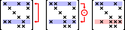
(a) Elementary stabilized transformation

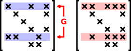
(b) Givens rotation

Figure 1: A comparison of the effect that an elementary stabilized transformation has on the sparsity structure to the effect of a Givens rotation. Here, $k=5$, $j=1$, and the elementary stabilized transformation exchanges rows $k$ and $j$ before eliminating element $(k,j)$.

The stabilized-elementary variant performs fewer arithmetic operations than the $QR$ variant. In the dense setting, elementary stabilized transformations require three times fewer arithmetic operations (because each elementary transformation is cheaper to perform than the corresponding Givens rotation). When the matrix is sparse, the effect can be much more dramatic, because fill that is not created in the lower triangle does not need to be eliminated (there are fewer transformations to apply) and because sparser rows mean that each transformation is cheaper.

We acknowledge that operation counts are not good predictors of running times on modern computers. To achieve fast running times, it is essential to exploit parallelism and to reduce communication. In sparse factorization, these optimizations are usually performed by exploiting elimination-tree parallelism,[jess82] and by invoking dense subroutines on submatrices that are full or almost full (supernodes[liu93]). Our implementation of the algorithm does not currently include such optimizations; implementing them is a significant research/engineering effort which we have not undertaken (see, e.g., [chen08, duff04, gupta00, hogg10, hogg11, li05]). Nevertheless, our implementation does demonstrate the sparsity of the algorithm and suggests that a high-performance variant of this algorithm can achieve performance comparable to that of other modern sparse codes.

3.2 A Sparse Implementation

Our implementation of the algorithm follows the outline of Algorithm 2, modified so that we store and operate only on the nonzero elements of the matrix. We represent the matrix using a data structure that we call expandable compressed sparse row (ECSR), which is a modification of the standard compressed sparse row (CSR) layout.[davis06]*p 8 ECSR exploits the fact that the fill in our algorithm is bounded by the fill in sparse $QR$, and that the number of structural nonzeros in each row in the $R$ factor can be computed in almost linear time.[gilbert94] Our code uses the function rowcolcounts of the CHOLMOD library to compute the row-wise nonzero counts.[chen08]

ECSR stores the nonzero elements and their column indices one row after another. The amount of space that we allocate to row $i$ is equal to the computed number of nonzeros in $R_{i,:}$, the $i$th row in the matrix’s $R$ factor (if $A_{i,:}$ is denser than $R_{i,:}$, we allocate enough space for $A_{i,:}$). This guarantees that the space allocated to row $i$ is sufficient to store row $i$ of $R$ and of all the intermediate upper-trapezoidal matrices. The representation consists of the following four vectors:

val

numerical values of the nonzeros (in all the rows)

col

column indices of the nonzeros (in all the rows)

head

pointers into val and col indicating where each row of the matrix starts

tail

pointers indicating where each row ends.

The vacant space of row $i$ is stored in positions tail[i] through head[i + 1].

We use one of two additional data structures to perform row eliminations. In the Givens variant of the algorithm, we use a two-row Sparse Accumulator (SPA),[gilbert92] and in the elementary-stabilized variant, we use an Ordered Sparse Accumulator (OSPA).[gilbert99] A multiple-row SPA represents a set of $m$ sparse rows with a shared sparsity structure using an $m$-by-$n$ matrix spa.val, which holds the numerical values of the nonzeros, a length-$n$ vector spa.occupied whose elements indicate which columns of spa.val are nonzero, and also spa.col, a list of the column indices of the nonzeros. The OSPA is similar, except that spa.col is stored in a heap data structure,[cormen09]*Sec 6 which provides cheap access to the leftmost nonzero column.

In the Givens variant of the algorithm, we use the SPA to perform Givens rotations as follows.

1. We copy the two rows into the SPA one by one. We start with the nonzero elements of the first row, updating the corresponding elements of spa.val and spa.occupied and adding the column indices of the nonzeros into spa.col. Next we copy the second row in the same way, except that now we use spa.occupied to avoid duplicating column indices in spa.col.

2. We apply the rotation to each nonzero column, using the column indices in spa.col to enumerate the nonzero columns.

3. Finally, we copy the nonzero elements back into the ECSR data structure and restore the SPA to its initial state, using spa.col to enumerate elements of spa.occupied and spa.val that must be cleared.

In this implementation, the total amount of work is proportional to the number of floating-point operations that the Givens rotation performs.

The elementary-stabilized variant is more complex. We implemented it using several subroutines that operate on the ECSR data structure and on a one-row OSPA:

load

Loads a row of an ECSR matrix into an empty OSPA. This is similar to loading a row into an unordered SPA, but requires a build-heap operation[cormen09]*Section 6.3 on the array of column indices.

store

Copies the contents of an OSPA back into a row of an ECSR matrix.

retrieve-head

Returns the position and the numerical value of the leftmost nonzero element of an OSPA (but leaves it in the OSPA). If the OSPA is empty, returns a special indicator, which we denote $\bot$.

remove-head

Removes the leftmost nonzero element from an OSPA.

subtract

Subtracts a multiple of a row of an ECSR matrix from an OSPA. This is a routine operation on a SPA; on an OSPA, columns need to be inserted into the column array using a heap-insert operation.

swap

Exchanges the content of an OSPA with a row of an ECSR matrix.

Given these building blocks, the overall algorithm can be composed as shown in Algorithm 3.

Algorithm 3 The sparse stabilized-elementary transformations variant of the algorithm.

1:Input: a symmetric ECSR matrix $A\in\mathbb{R}^{n\times n}$.

2:Output: the number $\nu$ of negative eigenvalues of $A$.

3:

4:$\nu\leftarrow 0$

5:$s\leftarrow\text{empty OSPA of length }n$

6:for $i\leftarrow 1,2,\dotsc,n$ do

7:     $x\leftarrow 0$

8:     load($s$, $A_{i,:}$)

9:     $\left(j,A_{ij}\right)\leftarrow\texttt{retrieve-head(}s\texttt{)}$

10:     while $j\neq\bot$ and $j<i$ do

11:         if $\left|A_{jj}\right|<\left|A_{ij}\right|$ then

12:              swap($s$, $A_{j,:}$)

13:              $x\leftarrow x+1$

14:              if $\operatorname{sign}(A_{jj})\neq\operatorname{sign}(A_{ij})$ then

15:                  $x\leftarrow x+1$

16:              end if

17:         end if

18:         subtract($s$, $\left(A_{ij}/A_{jj}\right)\cdot A_{j,:}$)

19:         remove-head($s$)

20:         $\left(j,A_{ij}\right)\leftarrow\texttt{retrieve-head(}s\texttt{)}$

21:     end while

22:     if $A_{ii}<0$ then

23:         $x\leftarrow x+1$

24:     end if

25:     if $x\bmod 2=1$ then

26:         $\nu\leftarrow\nu+1$

27:     end if

28:     store($s$, $A_{i,:}$)

29:end for

4 Numerical Analysis

Next, we describe the numerical behavior of the algorithm. The core numerical issue is explained in Wilkinson’s book.[wilkinson65]*p 312–315 We repeat this explanation below, for completeness, and also provide an example that shows how this numerical issue manifests itself.

The Givens variant of the algorithm is a thoroughly studied $QR$ factorization scheme and is known to compute backward-stable factors (see [higham02]*Sec 19). The elementary-stabilized version is not as well known, but it has also been analyzed in the literature. It has been called pairwise pivoting and was analyzed by Sorensen.[sorensen85] Sorensen’s analysis proves that the normwise backward error of the corresponding factorization is bounded by a product of four numbers: the magnitude of the elements of $A$, the unit roundoff $u$ ($2^{-53}\approx 1.1\times 10^{-16}$ in double-precision IEEE 754), and two growth factors. One of these growth factors represents the norm of the computed upper-triangular factor, and the other represents the norm of the implicit factor that is the equivalent of the $L$ factor in the $LU$ factorization with partial pivoting. In contrast with $LU$ with partial pivoting, this implicit factor is not lower triangular, and its elements are not bounded by 1 in magnitude. Sorensen proves in his paper that the two growth factors are bounded by $2^{n-1}-1$ and $2^{n-1}$, respectively. He also notes that although these bounds are large, they are highly pessimistic, and that large growth factors have not been encountered in practice. Further experimental evidence of this was provided by Grigori, Demmel and Xiang.[grigori11]*Fig 4.2

4.1 An Obstacle to a Backward-Stability Analysis

The backward stability of the $QR$ factorization and of pairwise pivoting implies that the factors that we obtain from our algorithm are backward stable. This applies to the final factors, but also to the intermediate ones that we obtain in each step. Stability can be hampered if the factorization suffers from growth, but large growth is rare. Because the algorithm uses the factors to compute the signs of the determinant sequence

$$1,\det(A_{1}),\det(A_{2}),\dotsc,\det(A_{n})\,,$$

the factors’ backward stability implies that each sign is backward stable. However, this does not imply the backward stability of the computed inertia. This is because each intermediate factor is modified in the steps that follow the step in which it is obtained, and therefore each sign of the determinant sequence has its own individual backward-error matrix (that equals the difference between $A$ and a matrix $\tilde{A}$ for which the factor is exact).

There is no reason to assume that if each factor is the exact factor of a matrix close to $A$, then they are all the factors of one matrix close to $A$, which would imply backward stability of the determinant sequence. Indeed, we can show that the algorithm is sometimes not backward stable.

4.2 An Example of Instability

Next, we show an example of how the algorithm can fail. We provide the transcript of a Matlab session, to make the example concrete.

We let $A$ be a square, symmetric $n$-by-$n$ matrix of the form

$$A=\,\begin{array}[]{c}\raisebox{1.0pt}{$\scriptstyle n/2$}\\ \raisebox{1.0pt}{$\scriptstyle n/2$}\end{array}\!\left[\begin{array}[]{cc}\mathchoice{\mathsm@sh\displaystyle{\overset{\text{\Large}\raisebox{1.0pt}{$\scriptstyle n/2$}}{\vphantom{Z^{T}}X}}}{\mathsm@sh\textstyle{\overset{\text{\Large}\raisebox{1.0pt}{$\scriptstyle n/2$}}{\vphantom{Z^{T}}X}}}{\mathsm@sh\scriptstyle{\overset{\text{\Large}\raisebox{1.0pt}{$\scriptstyle n/2$}}{\vphantom{Z^{T}}X}}}{\mathsm@sh\scriptscriptstyle{\overset{\text{\Large}\raisebox{1.0pt}{$\scriptstyle n/2$}}{\vphantom{Z^{T}}X}}}&\mathchoice{\mathsm@sh\displaystyle{\overset{\text{\Large}\raisebox{1.0pt}{$\scriptstyle n/2$}}{Z^{T}}}}{\mathsm@sh\textstyle{\overset{\text{\Large}\raisebox{1.0pt}{$\scriptstyle n/2$}}{Z^{T}}}}{\mathsm@sh\scriptstyle{\overset{\text{\Large}\raisebox{1.0pt}{$\scriptstyle n/2$}}{Z^{T}}}}{\mathsm@sh\scriptscriptstyle{\overset{\text{\Large}\raisebox{1.0pt}{$\scriptstyle n/2$}}{Z^{T}}}}\\ Z&0\\ \end{array}\right]$$

The leading diagonal block has the form

$$X=Q\,\operatorname{diag}(1,\epsilon_{1},\epsilon_{2},\dotsc,\epsilon_{n/2-1})\;Q^{T}\,,$$

where $Q$ is a random orthogonal matrix, and $\epsilon_{1},\epsilon_{2},\dotsc,\epsilon_{n/2-1}$ are random, independent, and normally distributed scalars with mean 0 and a standard deviation that equals the unit roundoff. The notation $\operatorname{diag}(\,\cdot\,)$ indicates a diagonal matrix with the specified diagonal elements. The block $Z$ is defined so that its elements are random, independent, and normally distributed with mean 0 and standard deviation 1.

In Matlab, we construct this matrix as follows:

• >> n = 2048;

  >> Q = orth(randn(n / 2));

  >> d = [1; eps * randn(n / 2 - 1, 1)];

  >> X = Q * diag(d) * Q’;

  >> Z = randn(n / 2);

  >> A = [X Z’; Z zeros(n / 2)];

Next, we compute $A$’s eigenvalues by running the Matlab command eig. Using these eigenvalues, we compute the matrix’s condition number and its negative index of inertia:

• >> ev = eig(A);

  >> kappa = max(abs(ev)) / min(abs(ev))

  kappa = 3.4498e+03

  >> nu = sum(ev < 0)

  nu = 1024

In this example, the eig command calls LAPACK’s symmetric eigensolver,[anderson99] which is backward stable. Its backward stability guarantees that the computed eigenvalues, condition number, and negative index of inertia are those of some matrix $\tilde{A}$ close to $A$. As we see above, the condition number is small, and so all of the matrices in the vicinity of $\tilde{A}$, including $A$ itself, have eigenvalues with the same signs as $\tilde{A}$. This means that all such matrices have the same negative index of inertia, namely $1{,}024$.

The inertia algorithm produces a different result:

• >> our_nu = inertia(A)

  our_nu = 1026

This shows that the algorithm is not backward stable. Any backward-stable algorithm would return the negative index of inertia of a matrix in the vicinity of $A$ and $\tilde{A}$, which must be $1{,}024$.

The result is similar regardless of whether we use the Givens variant of the algorithm or the elementary-stabilized one. In particular, because growth is not possible in the Givens variant, this shows that the instability is not caused by growth.

4.3 Instability Is Caused by Near Singularity

The cause of the instability is singularity of the leading principal minors. In our $A$, almost all of the leading principal submatrices have a condition number of order $u^{-1}$, where $u$ is the unit roundoff. The only exceptions are the three submatrices of orders 1, $n-1$ and $n$. Because the other $n-3$ submatrices are nearly singular, the computed signs of their determinants are often incorrect, even when computed using a backward-stable algorithm, and therefore counting the number of sign changes in the determinant sequence yields an incorrect result.

4.4 The (Limited) Effect of the Instability on Bisection

In the experiments that we describe in the next section, the eigenvalues that we produce using bisection are usually as accurate as those that we produce using a backward-stable eigensolver. The instability of the inertia algorithm does not appear to have an effect on bisection.

The reason for this is that the instability manifests itself only when $A-xI$ has a leading principal submatrix that is nearly singular. To make one of these submatrices nearly singular, $x$ must be at a distance of $O(u)\|A\|$ from an eigenvalue of such a submatrix. This can happen under two scenarios. First, as bisection converges to an eigenvalue of $A$, the point $x$ moves progressively closer to that eigenvalue until it reaches within $O(u)\|A\|$. This scenario does not create a problem, because when $x$ is close to an eigenvalue of $A$, an error in the computed inertia cannot prevent bisection from converging.[wilkinson65]*p 302–305 The other scenario is that $x$ is close to an eigenvalue of a leading principal submatrix of $A$, and that eigenvalue is far from every eigenvalue of $A$. This can lead bisection to fail. However, such unfortunate positioning of $x$ appears to happen only in pathological cases, meaning that the instability has few opportunities to have an effect.

5 Numerical Experiments

We carried out extensive numerical experiments to test the accuracy of the algorithm. In these experiments, we used our inertia algorithm as part of a bisection eigensolver to compute the eigenvalues of a variety of matrices. Although in practice bisection is often not a competitive algorithm, it requires a large number of inertia computations, and this makes it a convenient platform to stress-test our algorithm.

We computed the eigenvalues of two families of matrices. The first family is one that we produced using the LAPACK subroutine LATMS, which generates random dense matrices for testing LAPACK subroutines. These matrices have the form $A=Q\Lambda Q^{T}$, where $Q$ is a random orthogonal matrix and $\Lambda$ is a diagonal matrix whose diagonal elements $\lambda_{1},\lambda_{2},\dotsc,\lambda_{n}$ are the eigenvalues of $A$. The eigenvalues are randomly distributed according to two parameters named mode and $\kappa$. There are six possible modes, in the first five of which the eigenvalues have the form $\lambda_{i}=s_{i}\sigma_{i}$, where the scalars $s_{i}$ take the values $\pm 1$ independently with equal probability, and the scalars $\sigma_{i}$ have a distribution that depends on the mode. In all of the distributions that correspond to the first five modes, the $\sigma_{i}$ are nonnegative, and therefore they are the singular values of $A$. The distributions are the following:

1. The first singular value is equal to 1, and all others are equal to $1/\kappa$.

2. The first $n-1$ singular values are equal to 1, and $\sigma_{n}=1/\kappa$.

3. The singular values are evenly distributed between 1 and $1/\kappa$, on a logarithmic scale.

4. The singular values are evenly distributed between 1 and $1/\kappa$, on a linear scale.

5. The singular values have the form $\left(1/\kappa\right)^{e}$, where $e$ is drawn independently for each singular value from the uniform distribution on the interval $\left(0,1\right)$.

Finally, in mode 6, LATMS generates the $\lambda_{i}$ directly without generating the singular values first. In this mode, the $\lambda_{i}$ are independent and normally distributed with mean 0 and standard deviation 1.

We generated one matrix of order $n=256$ for each combination of mode and $\kappa$, for various values of $\kappa$, and computed all of the eigenvalues of that matrix. We then measured their accuracy using the maximal normalized error,

$$\max_{i=1,2,\dotsc,n}|\lambda_{i}-\hat{\lambda}_{i}|/\|A\|_{1}\,,$$ (1)

where the $\lambda_{i}$ are the actual eigenvalues used by LATMS and the $\hat{\lambda}_{i}$ are the approximate ones produced by our bisection eigensolver. The full results are shown in Table 1. All of the errors are within one order of magnitude from $u\approx 1.1\times 10^{-16}$.

Table 1: Accuracy of the computed eigenvalues of random dense matrices, generated using the LAPACK subroutine LATMS.

	maximal error
mode	$\kappa=$1\text{\times}{10}^{01}$$	$\kappa=$1\text{\times}{10}^{04}$$	$\kappa=$1\text{\times}{10}^{08}$$	$\kappa=$1\text{\times}{10}^{12}$$	$\kappa=$1\text{\times}{10}^{16}$$
1	$7.731\,672\,221\,44\text{\times}{10}^{-16}$	$7.021\,204\,431\,43\text{\times}{10}^{-16}$	$4.910\,398\,043\,67\text{\times}{10}^{-16}$	$2.073\,467\,328\,12\text{\times}{10}^{-16}$	$1.748\,713\,755\,87\text{\times}{10}^{-15}$
2	$8.988\,832\,937\,29\text{\times}{10}^{-16}$	$7.498\,408\,631\,4\text{\times}{10}^{-16}$	$1.889\,376\,686\,22\text{\times}{10}^{-15}$	$5.260\,366\,874\,4\text{\times}{10}^{-16}$	$1.783\,853\,752\,3\text{\times}{10}^{-15}$
3	$1.746\,176\,856\,68\text{\times}{10}^{-15}$	$1.757\,360\,968\,06\text{\times}{10}^{-15}$	$2.119\,839\,859\,13\text{\times}{10}^{-15}$	$1.734\,027\,127\,32\text{\times}{10}^{-15}$	$1.758\,056\,879\,76\text{\times}{10}^{-15}$
4	$1.774\,882\,223\,97\text{\times}{10}^{-15}$	$1.848\,332\,415\,87\text{\times}{10}^{-15}$	$1.834\,911\,025\,8\text{\times}{10}^{-15}$	$1.821\,419\,039\,92\text{\times}{10}^{-15}$	$1.788\,509\,346\,23\text{\times}{10}^{-15}$
5	$1.821\,856\,801\,27\text{\times}{10}^{-15}$	$1.766\,381\,332\,79\text{\times}{10}^{-15}$	$1.779\,631\,680\,04\text{\times}{10}^{-15}$	$1.766\,970\,580\,3\text{\times}{10}^{-15}$	$1.782\,028\,664\,92\text{\times}{10}^{-15}$
6a,b	$1.825\,317\,196\,33\text{\times}{10}^{-15}$	$1.825\,317\,196\,33\text{\times}{10}^{-15}$	$1.825\,317\,196\,33\text{\times}{10}^{-15}$	$1.825\,317\,196\,33\text{\times}{10}^{-15}$	$1.825\,317\,196\,33\text{\times}{10}^{-15}$

• Matrices generated in mode 6 do not depend on $\kappa$, and therefore all of the entries in the bottom row represent the same matrix.

• The frequent appearance of the number $1.8\times 10^{-15}$ in the first five rows is an artifact of rounding to two significant digits; actual numbers are all distinct.

The second family of matrices in our experiments are sparse matrices from the SuiteSparse Matrix Collection.[davis11b] We first computed the inertia of all 283 real symmetric matrices of order $64<n<16{,}384$ in this collection whose elements have known numerical values. Each inertia computation was carried out on a single core of an Intel i7-2600 CPU, with our code compiled using version 13.1.1 of the Intel compiler suite. We then used this computation as follows to winnow down our list of matrices. The analysis of bisection in Section 2.3 indicates that the time required to compute all of the eigenvalues of $A$ to double-precision accuracy is at most $-\log(u)\,n\,T(A)$, where $u$ is double-precision unit roundoff, $n$ is the order of $A$, and $T(A)$ is the time required to compute $A$’s inertia once. We selected all of the matrices for which this estimate was at most 2 hours, and ran bisection to compute all of the eigenvalues of each such matrix. In total, we ran bisection on 116 matrices, described below in Table 2.

As in the previous experiment, we computed the eigenvalues of each of the 116 matrices, and measured the maximal normalized error (1) relative to backward-stable eigenvalues computed using the LAPACK subroutine SYEV. The results are shown in a histogram plot in Figure 2. The errors are again comparable to $u$, ranging between $8.0\times 10^{-16}$ and $3.5\times 10^{-14}$, with a median of $3.5\times 10^{-15}$.

Table 2: Statistical parameters of the set of SuiteSparse matrices.

	$n$	$\mathtt{nnz}/n$	$\kappa$
minimum	$66.0$	$0.457,361,642,882$	$4.965\,95$
1st quartile	$380.0$	$3.75$	$7288.1$
median	$958.5$	$6.889,443,795,67$	$1.589\,65\text{\times}{10}^{06}$
3rd quartile	$1920.5$	$16.771,568,241,7$	$7.542\,33\text{\times}{10}^{10}$
maximum	$15,439.0$	$97.322,580,645,2$	inf

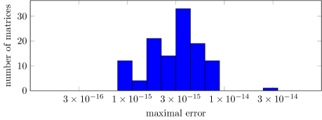
Figure 2: Accuracy of the computed eigenvalues of sparse matrices from the SuiteSparse collection.

6 Performance Experiments

In this section, we describe the experiments that we carried out to study the performance of our sparse inertia algorithm. We analyzed the performance of the two variants of our algorithm, and we compared it with the performance of two other factorization algorithms. The first algorithm that we compared ourselves with is SuiteSparseQR, or SPQR for short.[davis11a] It is a state-of-the-art sparse $QR$ factorization algorithm, and it is the algorithm that runs when we apply Matlab’s qr command to a sparse matrix. Our interest in SPQR stems from the fact that it computes the same factorization that we compute in the Givens variant of our algorithm. Comparing ourselves with SPQR helps us to learn how much performance we can gain by adopting the advanced techniques that are implemented in SPQR, such as the use of supernodes.

The second algorithm with which we compared ourselves is the algorithm MA57 from the HSL library.[duff04, hsl] It is an industrial-quality sparse-factorization algorithm for symmetric-indefinite matrices. An important distinction between SPQR and MA57 is that the former does not compute the inertia, while the latter does. In these experiments, MA57 represents the alternative to our approach to the problem of computing the inertia. A comparison with MA57 allows us to gain insight into the relative strengths and weaknesses of our algorithm.

We carried out two experiments on a single core of an Intel Xeon E5-2650 v3 CPU, using gcc and gfortran version 6.2.0, Intel MKL version 11.3.1, SuiteSparse version 4.5.3, and MA57 version 3.8.0. We use the default settings for all algorithms. In particular, this means that MA57 pre-scales the matrix so as to reduce the need for pivoting, which is something our algorithm does not do.

Our first experiment was carried out on a set of 81 matrices from the SuiteSparse Matrix Collection. The matrices were chosen by selecting all of the symmetric, real, indefinite matrices of order $32{,}768\leq n\leq 65{,}536$. For each matrix, we computed a nested-dissection ordering for $A$ using METIS, and then applied each of the algorithms to the reordered matrix. We discarded 21 matrices for which at least one factorization took more than one hour or required more than 16 GB of memory; this left us with a set of 60 matrices.

Figure 3 compares the performance of the Givens variant of our algorithm to that of SPQR. We find that the required number of arithmetic operations (flops) in the two algorithms is within a factor of 10 of each other, with no significant advantage in favor of either one. The reason for the variation in flops is because the two algorithms process the rows in different orders, and the order of the rows can have a dramatic effect on flops. This has already been noted by George and Heath.[george80]*p 78 The computational rate of SPQR is however much higher, ranging between 1.1 and 10 gflop/s, whereas that of our algorithm ranges between 151 and 874 mflop/s. This also translates to a dramatic difference in running times in favor of SPQR.

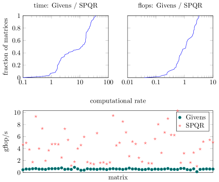
Figure 3: A comparison of the Givens variant of our algorithm with SPQR. The top plots show two empirical cumulative-distribution-function curves of the ratio of the running time of our algorithm to that of SPQR (left) and the ratio of the numbers of arithmetic operations of the two algorithms (right). The bottom plot shows the computational rates of the two algorithms.

Figure 4 shows that the elementary-stabilized variant of the algorithm is much more efficient than the Givens variant. The elementary-stabilized variant performs a factor of 0.001 to 0.13 of the flops that the Givens variant performs. The computational rates of the two codes are comparable, with some outliers that we ascribe to the cost of row interchanges in the elementary-stabilized case. The elementary-stabilized version is therefore faster by a significant factor, between 3.14 and 269.

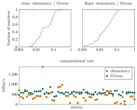
Figure 4: A comparison of the two variants of our algorithm using the same type of plots as in Figure 3.

Figure 5 compares the elementary-stabilized variant with SPQR. Although, as we have seen in the previous figures, the computational rate of our algorithm is orders of magnitude lower, we preserve sparsity much better. Our algorithm always performs fewer flops than SPQR, with a median ratio of 0.017. Due to the much better sparsity, we are actually faster in 42 of the 60 matrices, with a time ratio that ranges between 0.0011 and 3.64.

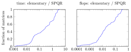
Figure 5: A comparison of the elementary-stabilized variant of our algorithm with SPQR. (The computational rates of the two algorithms are presented in Figures 3 and 4.)

Finally, Figure 6 compares the performance of the elementary-stabilized variant with MA57. We see that MA57 is better than our algorithm at preserving sparsity, requiring up to a factor of 21.7 fewer flops than our algorithm. MA57 also achieves a significantly faster computational rate of up to 18.55 gflop/s, although in 33 of the matrices it falls below 1 gflop/s and can be as low as 51 mflop/s. Nevertheless, MA57 is faster in all but 3 matrices, with a speedup that ranges between 0.75 and 333.

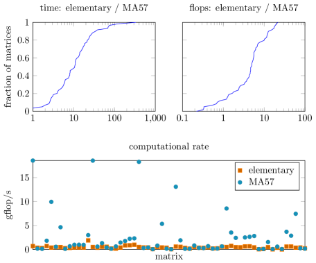
Figure 6: A comparison of the elementary-stabilized variant of our algorithm with MA57.

In this experiment, we found two matrices for which our algorithm and MA57 did not return the same inertia. The first matrix is AG-Monien/shock-9, for which both versions of our algorithm returned a negative index of inertia of 18,168, and MA57 returned 18,178. According to the annotation in the SuiteSparse collection, this matrix has a nullspace of dimension 137, so the discrepancy is not surprising. The second matrix is AG-Monien/se, which has a nullspace of dimension 457, and for which our elementary-transformation based algorithm returned 16,215, while the Givens-rotation version and MA57 returned 16,175.

In our final experiment, we made a more detailed comparison of our algorithm with MA57. Our goal is to find matrices where our more conservative approach pays off. We started with the 422 symmetric, real, indefinite matrices of order $8{,}192\leq n\leq 1{,}048{,}576$ in the SuiteSparse collection, but kept only the 54 matrices whose MA57 factor had at least twice as many nonzeros as the Cholesky factor would have contained (had the matrix been positive definite). This produced a set of matrices on which pivoting in MA57 caused significant fill. For each of the 54 matrices, we invoked our factorization and MA57 using two orderings: an optimistic nested-dissection ordering of $A$ and a conservative nested-dissection ordering of the structure of $A^{T}A$. We then compared MA57 and our algorithm with respect to a parameter we refer to as fill, which we define as the number of nonzeros in the triangular factor, divided by the number of nonzeros in $A$. We omit the results for MA57 using an $A^{T}A$ ordering because MA57 always produced less fill with an $A$ ordering than with an $A^{T}A$ ordering. In 19 of the matrices we found that the fill in our algorithm is lower than the fill of MA57, sometimes dramatically so. A list of these matrices is given in Table 3.

Table 3: Matrices for which our algorithm with one of the orderings produced less fill than MA57. We define fill as the number of nonzero elements in the triangular factor, divided by the number of nonzeros in $A$. Column headings nd and wide indicate nested-dissection ordering of $A$ and of $A^{T}A$ respectively (the latter of the two is equivalent to a wide-separator nested-dissection ordering of $A$). The symbol $\dagger$ indicates that the computation exceeded the maximal allocated time of one hour, and $\ddagger$ indicates that the algorithm required more memory than the allocated 16 GB.

			fill
			MA57	our algorithm
matrix name	$n$	$\mathtt{nnz}/n$		nd	wide
AG-Monien/3elt_dual	$9,000$	$2.9507$	$9.4798$	$11.3902$	$6.8534$
AG-Monien/big_dual	$30,269$	$2.9686$	$11.0017$	$13.8358$	$8.1708$
AG-Monien/crack_dual	$20,141$	$2.9833$	$8.2900$	$11.1016$	$7.3660$
AG-Monien/L-9	$17,983$	$3.9589$	$14.1623$	$13.8729$	$10.6758$
AG-Monien/whitaker3_dual	$19,190$	$2.9787$	$11.8616$	$16.8701$	$10.1071$
Andrianov/net150	$43,520$	$71.7188$	‡	$33.9815$	†
Andrianov/pattern1	$19,242$	$484.5355$	$7.2023$	$5.6382$	$9.4272$
DIMACS10/t60k	$60,005$	$2.9811$	$12.7535$	$20.0771$	$10.9359$
GHS_indef/dtoc	$24,993$	$2.7997$	$4.0359$	$3.3634$	$1.8226$
Gleich/usroads	$129,164$	$2.5616$	$5.4667$	$4.8758$	$3.9858$
Gleich/usroads-48	$126,146$	$2.5677$	$5.5008$	$4.9328$	$4.0602$
Gset/G66	$9,000$	$4.0000$	$16.3408$	$26.3351$	$14.3614$
Gset/G67	$10,000$	$4.0000$	$15.9896$	$27.0603$	$14.1767$
Gupta/gupta3	$16,783$	$555.5280$	$6.5575$	$4.9891$	$11.5356$
Rajat/rajat06	$10,922$	$4.3017$	$6.1684$	$5.0437$	$3.8255$
Rajat/rajat07	$14,842$	$4.3062$	$6.3074$	$5.6055$	$3.9817$
Rajat/rajat08	$19,362$	$4.3096$	$6.5421$	$5.6489$	$4.3172$
Rajat/rajat09	$24,482$	$4.3123$	$6.6991$	$6.3744$	$4.5102$
Rajat/rajat10	$30,202$	$4.3144$	$6.6424$	$6.2713$	$4.7733$

As in the previous experiment, we found six matrices for which the different algorithms did not return the same inertia. Of these matrices, two are identified by the SuiteSparse matrix collection as having a high-dimensional nullspace; three are large matrices for which the dimension of the nullspace is not known, but all three are binary; and finally, the matrix GHS_index/bratu3 is nonsingular but has the same features as the example of Section 4. The details are in Table 4.

Table 4: The computed negative index of inertia for matrices on which the two algorithms did not return the same value.

	MA57	our algorithm
matrix name		nd	wide
AG-Monien/shock-9	$18,178$	$18,168$	$18,168$
GHS_indef/bratu3d	$12,167$	$12,143$	$12,167$
Gleich/usroads-48	$62,932$	$62,931$	$62,931$
Gupta/gupta3	$1,264$	$1,264$	$1,266$
DIMACS10/caidaRouterLevel	$70,082$	‡	$70,080$
DIMACS10/fe_ocean	$71,719$	$71,684$	$71,713$

7 Discussion and Conclusions

In this paper, we proposed a sparse variant of Wilkinson’s inertia algorithm. The new inertia algorithm provides provable a priori bounds on the fill, which other algorithms do not provide.

Our performance experiments show that even without using the techniques that are necessary to obtain top performance from a sparse-matrix algorithm (such as using supernodes), our algorithm is competitive and often superior to a top-quality sparse $QR$ factorization code due to the sparser factors that we produce in our algorithm.

Nevertheless, our algorithm is usually slower than MA57, often much slower. Due to the use of supervariables in MA57, it achieves much higher computational rates, and thanks to its use of threshold pivoting and a matching algorithm that allows it to rescale the matrix so as to prevent pivoting,[duff05] it is better able to preserve sparsity. For matrices that do not require significant pivoting, disabling matching-based rescaling can further improve MA57’s performance. Other ordering methods, such as minimum degree, can produce less fill and thus yield further gains. These techniques can be used in our algorithm as well, and we expect significant improvement if they are used. Even without this, we found several cases where our approach yields less fill, and one matrix (Andrianov/net150) that MA57 cannot factor within the allotted time and space, whereas we can.