KIAS-P15060

$h,Z\to\ell_{i}\bar{\ell}_{j}$, $\Delta a_{\mu}$, $\tau\to(3\mu,\mu\gamma)$ in generic two-Higgs-doublet models

Abstract

Inspired by a significance of $2.4\sigma$ for the $h\to\mu\tau$ decay observed by the CMS experiment at $\sqrt{s}=8$ TeV, we investigate the Higgs lepton-flavor-violating effects in a generic two-Higgs-doublet model (THDM), where the lepton-flavor-changing neutral currents are induced at the tree level and arise from Yukawa sector. We revisit the constraints for generic THDM by considering theoretical requirements, precision measurements of $\delta\rho$ and oblique parameters $S$, $T$, and $U$, and Higgs measurements. The bounds from Higgs data play the major limits. With parameter values that simultaneously satisfy the Higgs bounds and the CMS excess of the Higgs coupling to $\mu$-$\tau$, we find that the tree-level $\tau\to 3\mu$ and the loop-induced $\tau\to\mu\gamma$ decays are consistent with current experimental upper limits; the discrepancy in muon $g-2$ between experimental results and standard model predictions can be resolved, and an interesting relation between muon $g-2$ and the branching ratio (BR) for $\mu\to e\gamma$ is found. The generic THDM results show that the order of magnitude of the ratio $BR(h\to e\tau)/BR(h\to\mu\tau)$ is smaller than $10^{-4}$. Additionally, we also study the rare decay $Z\to\mu\tau$ and get $BR(Z\to\mu\tau)<10^{-6}$.

The observed-flavor-changing neutral currents (FCNCs) in the standard model (SM) occur at the loop level of the quark sector and originate from $W$-mediated charged currents, such as $K-\bar{K}$, $B-\bar{B}$, and $D-\bar{D}$ mixings and $b\to s\gamma$. Due to the loop effects, it is believed that these FCNC processes are sensitive to new physics. However, most of these processes involve large uncertain non-perturbative quantum chromodynamics (QCD) effects; therefore, even if new physics exist, it is not easy to distinguish them from the SM results due to QCD uncertainty.

The situation in the lepton sector is different. Although the SM also has lepton FCNCs (e.g., $\mu\to e\gamma$ and $\tau\to(e,\mu)\gamma$) they are irrelevant to QCD effects and highly suppressed; if any signal is observed, it is certainly strong evidence for new physics. It is thus important to search for new physics through the lepton sector Crivellin:2013wna ; Gomez:2014uha ; Crivellin:2015hha .

With the discovery of a new scalar with a mass of around 125 GeV at the ATLAS :2012gk and CMS :2012gu experiments, we have taken one step further toward understanding the electroweak symmetry breaking (EWSB) through spontaneous symmetry breaking (SSB) mechanism in the scalar sector. With $\sqrt{s}=13-14$ TeV, the next step for the High Luminosity Large Hadron Collider (LHC) is to explore not only the detailed properties of the observed scalar, but also the existence of other Higgs scalars and new physics effects.

CMS Khachatryan:2015kon and ATLAS Aad:2015gha have recently reported the measurements of $h\to\mu\tau$ decay in $pp$ collisions at $\sqrt{s}=8$ TeV. At the $95\%$ confidence level (CL), the branching ratio (BR) for the decay at CMS is $BR(h\to\mu\tau)<1.51\%$ and that at ATLAS is $BR(h\to\mu\tau)<1.85\%$ . Additionally, a slight excess of events with a significance of $2.4\sigma$ was reported by CMS, with the best fit of $BR(h\to\mu\tau)=(0.84^{+0.39}_{-0.37})\%$. If the excess is not a statistical fluctuation, the extension of the SM becomes necessary. Inspired by the excess of events, possible new physics effects have been studied Campos:2014zaa ; Sierra:2014nqa ; Lee:2014rba ; Heeck:2014qea ; Crivellin:2015mga ; Dorsner:2015mja ; Omura:2015nja ; Crivellin:2015lwa ; Das:2015zwa ; Bishara:2015cha ; Varzielas:2015joa ; He:2015rqa ; Chiang:2015cba ; Altmannshofer:2015esa ; Cheung:2015yga ; Arganda:2015naa ; Botella:2015hoa ; Baek:2015mea ; Huang:2015vpt ; Baek:2015fma ; Arganda:2015uca ; Aloni:2015wvn . The earlier relevant works have been investigated Arganda:2004bz ; Blankenburg:2012ex ; Arhrib:2012mg ; Harnik:2012pb ; Dery:2013rta ; Arana-Catania:2013xma ; Arroyo:2013tna ; Celis:2013xja ; Falkowski:2013jya ; Arganda:2014dta ; Dery:2014kxa .

Following the measurements of ATLAS and CMS of the couplings of Higgs to leptons, we investigate the lepton flavor violation (LFV) in a generic two-Higgs-doublet model (THDM) Lee:1973iz . The THDM includes five physical scalar particles, namely two CP-even bosons, one CP-odd pseudoscalar, and one charged Higgs boson. According to the form in which Higgs doublets couple to fermions, the THDM is classified as type I, II, and III models, lepton-specific model, and flipped model Branco:2011iw . The minimal supersymmetric SM (MSSM) belongs to the type II THDM, in which one Higgs doublet couples to up-type quarks while the other couples to down-type quarks. The type III THDM corresponds to the case in which each of the two Higgs doublets couples to all fermions simultaneously. As a result, tree-level FCNCs in the quark and charged lepton sectors are induced. Considering the strict experimental data, it is interesting to determine the impacts of the type III model on the LFV.

If we assume no new CP-violating source from the scalar sector, such as the type II model and MSSM, the main new free parameters are the masses of new scalars, $\tan\beta=v_{2}/v_{1}$ and angle $\alpha$, where $\tan\beta$ is related to the ratio of the vacuum expectation values (VEVs) of two Higgs fields and the angle $\alpha$ stands for the mixing effect of two CP-even scalars. Basically, these two parameters have been strictly constrained by the current experimental data, such as $\rho$-parameter, $S$, $T$, and $U$ oblique parameters, Higgs searches through $h\to(\gamma\gamma,WW^{*},ZZ^{*},\tau\tau,b\bar{b})$, etc. In order to show the correlation of free parameters and these experimental bounds, we revisit the constraints by adopting the $\chi$-square fitting approach. it can be seen that although the allowed values of $\cos(\beta-\alpha)$ approach the decoupling limit (i.e., $\alpha\sim\beta-\pi/2$) if $\cos\beta$ is sufficiently small, the BR for $h\to\mu\tau$ could still be as large as the measurements from ATLAS and CMS.

Besides the $h\to\ell_{i}\bar{\ell}_{j}$ decays, the type III model has also significant effects on other lepton-flavor-conserving and -violating processes, such as muon anomalous magnetic moment, $\mu\to 3e$, $\mu(\tau)\to e(\mu,e)\gamma$, $Z\to\ell_{i}\bar{\ell}_{j}$, etc. Although concrete signals for lepton-flavor-violating processes have not been observed yet, the current experimental data with $BR(\mu\to 3e)<10^{-12}$ and $BR(\mu\to e\gamma)<5.7\times 10^{-13}$ PDG have put strict limits on $\mu\to 3e$ and $\mu\to e\gamma$, respectively. Combing the LHC data and the upper limits of the rare lepton decays, we study whether the excess of muon $g-2$ can be resolved and whether the BRs of the listed lepton FCNC processes are consistent with current data in the type III THDM.

To indicate the scalar couplings to fermions in the type III model, we express the Yukawa sector as:

$$-{\cal L}_{Y} = \bar{Q}_{L}Y^{u}_{1}U_{R}\tilde{H}_{1}+\bar{Q}_{L}Y^{u}_{2}U_{R}\tilde{H}_{2}$$ (1)

$$+ \bar{Q}_{L}Y^{d}_{1}D_{R}H_{1}+\bar{Q}_{L}Y^{d}_{2}D_{R}H_{2}$$

$$+ \bar{L}Y^{\ell}_{1}\ell_{R}H_{1}+\bar{L}Y^{\ell}_{2}\ell_{R}H_{2}+h.c.\,,$$

where we have hidden all flavor indices, $Q^{T}_{L}=(u,d)_{L}$ and $L^{T}=(\nu,\ell)_{L}$ are the $SU(2)_{L}$ quark and lepton doublets, respectively, $Y^{f}_{1,2}$ are the Yukawa matrices, $\tilde{H}_{i}=i\tau_{2}H^{*}_{i}$ with $\tau_{2}$ being the second Pauli matrix, the Higgs doublets are represented by:

$$H_{i} = \left(\begin{array}[]{c}\phi^{+}_{i}\\ (v_{i}+\phi_{i}+i\eta_{i})/\sqrt{2}\\ \end{array}\right)\,,$$ (4)

and $v_{i}$ is the VEV of $H_{i}$. Equation (1) can recover the type II THDM if $Y^{u}_{1}$, $Y^{d}_{2}$, and $Y^{\ell}_{2}$ vanish. Before EWSB, all $Y^{f}_{1,2}$ are arbitrary $3\times 3$ matrices and fermions are not physical eigenstates; therefore, we have the freedom to choose $Y^{u}_{1}$, $Y^{d}_{2}$, and $Y^{\ell}_{2}$ to have diagonal forms; that is, $Y^{u}_{1}={\rm diag}(y^{u}_{1},y^{u}_{2},y^{u}_{3})$ and $Y^{d,\ell}_{2}={\rm diag}(y^{d,\ell}_{1},y^{d,\ell}_{2},y^{d\ell}_{3})$.

By the measurements of neutrino oscillations, it is known that the SM neutrinos are massive particles. Since the origin of neutrino masses is not conclusive, in order to introduce the neutrino masses and avoid changing the structure of scalar interactions in the THDM, the neutrino masses can be generated through the type-I seesaw mechanism T1seesaw . If we include three heavy right-handed neutrinos, the associated Yukawa couplings are given by:

$$-Y_{N}=\left(\bar{L}\left({\bf y}_{1}\tilde{H}_{1}+{\bf y}_{2}\tilde{H}_{2}\right)N+h.c.\right)+\frac{1}{2}{\cal N}^{T}C{\bf m}_{N}{\cal N}\,,$$ (5)

where we have suppressed the flvaor indices, ${\cal N}_{i}=N_{i}$ stands for the heavy right-handed neutrino, and diag${\bf m}_{N}=(m_{N1},m_{N2},m_{N3})$ in flavor space. Accordingly, the neutrino mass matrix is expressed as:

$$m_{\nu}=\left(\begin{array}[]{cc}\mathbb{0}&({\bf y}_{1}v_{1}+{\bf y}_{2}v_{2})/\sqrt{2}\\ ({\bf y}^{T}_{1}v_{1}+{\bf y}^{T}_{2}v_{2})/\sqrt{2}&{\bf m}_{N}\end{array}\right)\,.$$ (8)

By taking proper values of ${\bf m}_{N}$ and ${\bf y}_{1,2}$, we can fit the the measured mass-square differences, where the data are $\Delta m^{2}_{12}=(7.53\pm 0.18)\times 10^{-5}$ eV² and $\Delta m^{2}_{23}=(2.44\pm 0.06)\times 10^{(}-3)$ eV² for normal hierarchy, or $m^{2}_{23}=(1.52\pm 0.07)\times 10^{-3}$ eV² for inverted hierarchy PDG . Since the neutrino effects are irrelevant to the current study, hereafter we do not further discuss the detailed properties of neutrinos.

The VEVs $v_{1,2}$ are dictated by the scalar potential, where the gauge invariant form is given by Branco:2011iw :

$$V(\Phi_{1},\Phi_{2}) = m^{2}_{1}\Phi^{\dagger}_{1}\Phi_{1}+m^{2}_{2}\Phi^{\dagger}_{2}\Phi_{2}-(m^{2}_{12}\Phi^{\dagger}_{1}\Phi_{2}+{\rm h.c})+\frac{1}{2}\lambda_{1}(\Phi^{\dagger}_{1}\Phi_{1})^{2}$$ (9)

$$+ \frac{1}{2}\lambda_{2}(\Phi^{\dagger}_{2}\Phi_{2})^{2}+\lambda_{3}(\Phi^{\dagger}_{1}\Phi_{1})(\Phi^{\dagger}_{2}\Phi_{2})+\lambda_{4}(\Phi^{\dagger}_{1}\Phi_{2})(\Phi^{\dagger}_{2}\Phi_{1})$$

$$+ \left[\frac{\lambda_{5}}{2}(\Phi^{\dagger}_{1}\Phi_{2})^{2}+\left(\lambda_{6}\Phi^{\dagger}_{1}\Phi_{1}+\lambda_{7}\Phi^{\dagger}_{2}\Phi_{2}\right)\Phi^{\dagger}_{1}\Phi_{2}+{\rm h.c.}\right]\,.$$

Since we do not concentrate on CP violation, we set the parameters in Eq. (9) to be real numbers. In addition, we also require the CP phase that arises from the ground state to vanish Lee:1973iz . By the scalar potential with CP invariance, we have nine free parameters. In our approach, the independent parameters are taken as:

$$\{m_{h}\,,m_{H}\,,m_{A}\,,m_{H^{\pm}}\,,v\,,\tan\beta\,,\alpha\,,\lambda_{6}\,,\lambda_{7}\}$$ (10)

with $v=\sqrt{v^{2}_{1}+v^{2}_{2}}$.

With the nonvanished $\lambda_{6,7}$ terms in the potential, not only the mass relations of scalar bosons are modified but also the scalar triple and quartic couplings receive the changes. Since the masses of scalar bosons are treated as free parameters, the direct contributions of $\lambda_{6,7}$ to the process $h\to\gamma\gamma$ in this study are through the triple coupling $h$-$H^{+}$-$H^{-}$. By the constraint from $b\to s\gamma$, the mass of charged Higgs can not be lighter than 480 GeV; the contribution of the charged Higgs loop to the decay $h\to\gamma\gamma$ is small. That is, the influence of $\lambda_{6,7}$ on the constraint of parameter is not significant. Without loss of generality, in the phenomenological analysis, we set $\lambda_{6,7}\ll 1$. The detailed numerical study with $\lambda_{6,7}\sim{\cal O}(1)$ can be found elsewhere Arhrib:2015maa .

The physical states for scalars are expressed by:

$$h = -s_{\alpha}\phi_{1}+c_{\alpha}\phi_{2}\,,$$

$$H = c_{\alpha}\phi_{1}+s_{\alpha}\phi_{2}\,,$$

$$H^{\pm}(A) = -s_{\beta}\phi^{\pm}_{1}(\eta_{1})+c_{\beta}\phi^{\pm}_{2}(\eta_{2})$$ (11)

with $c_{\alpha}(s_{\alpha})=\cos\alpha(\sin\alpha)$, $c_{\beta}=\cos\beta=v_{1}/v$, and $s_{\beta}=\sin\beta=v_{2}/v$. In this study, $h$ is the SM-like Higgs while $H$, $A$, and $H^{\pm}$ are new particles in the THDM. Using Eqs. (1) and (4), one can easily find that the fermion mass matrix is

$${\bf M}_{f}=\frac{v}{\sqrt{2}}\left(\cos\beta Y^{f}_{1}+\sin\beta Y^{f}_{2}\right)\,.$$ (12)

If we introduce the unitary matrices $V^{f}_{L}$ and $V^{f}_{R}$, the mass matrix can be diagonalized through ${\bf m}_{f}=V^{f}_{L}{\bf M}_{f}V^{f\dagger}_{R}$. Accordingly, the scalar couplings to fermions could be formulated as:

$$-{\cal L}_{Y\phi} = \bar{\ell}_{L}\;\epsilon_{\phi}{\bf y}^{\ell}_{\phi}\;\ell_{R}\;\phi+\bar{\nu}_{L}V_{\rm PMNS}\;{\bf y}^{\ell}_{H^{\pm}}\;\ell_{R}\;H^{+}+h.c.\,,$$ (13)

where $\phi=h,H,A$ stands for the possible neutral scalar boson, $\epsilon_{h(H)}=1$, $\epsilon_{A}=i$, $V_{\rm PMNS}$ is the Pontecorvo-Maki-Nakagawa-Sakata matrix, and the Yukawa couplings ${\bf y}^{\ell}_{\phi,H^{\pm}}$ are defined by:

$$({\bf y}^{\ell}_{h})_{ij} =-\frac{s_{\alpha}}{c_{\beta}}\frac{m_{i}}{v}\delta_{ij}+\frac{c_{\beta\alpha}}{c_{\beta}}X^{\ell}_{ij}\,,$$

$$({\bf y}^{\ell}_{H})_{ij} =\frac{c_{\alpha}}{c_{\beta}}\frac{m_{i}}{v}\delta_{ij}-\frac{s_{\beta\alpha}}{c_{\beta}}X^{\ell}_{ij}\,,$$

$$({\bf y}^{\ell}_{A})_{ij} =-\tan\beta\frac{m_{i}}{v}\delta_{ij}+\frac{X^{\ell}_{ij}}{c_{\beta}}\,,$$ (14)

and ${\bf y}^{\ell}_{H^{\pm}}=\sqrt{2}{\bf y}^{\ell}_{A}$ with $c_{\beta\alpha}=\cos(\beta-\alpha)$, $s_{\beta\alpha}=\sin(\beta-\alpha)$ and

$${\bf X^{u}}=V^{u}_{L}\frac{Y^{u}_{1}}{\sqrt{2}}V^{u\dagger}_{R}\,,\ {\bf X^{d}}=V^{d}_{L}\frac{Y^{d}_{2}}{\sqrt{2}}V^{d\dagger}_{R}\,,\ {\bf X^{\ell}}=V^{\ell}_{L}\frac{Y^{\ell}_{2}}{\sqrt{2}}V^{\ell\dagger}_{R}\,.$$ (15)

From these formulations, it can be seen that the Yukawa couplings of Higgses to fermions can return to the type II THDM when $Y^{u}_{1}$ and $Y^{d,\ell}_{2}$ vanish. The FCNC effects are also associated with $Y^{u}_{1}$ and $Y^{d,\ell}_{2}$, which can be chosen to be diagonal matrices, as mentioned earlier. The detailed Yukawa couplings of $H$, $A$, and $H^{\pm}$ to up- and down-type quarks are summarized in the appendix.

In principle, $Y^{f}_{1,2}$ are arbitrary free parameters. In order to get more connections among parameters and reduce the number of free parameters, the hermitian Yukawa matrices can be applied, where the hermiticity of the Yukawa matrix can be realized by symmetry, such as global (gauged) horizontal $SU(3)_{H}$ symmetry Masiero:1998yi and left-right symmetry Babu:1999xf . Therefore, the equality $V^{f}_{L}=V^{f}_{R}\equiv V^{f}$ can be satisfied. With the diagonal $Y^{u}_{1}$ and $Y^{d,\ell}_{2}$, the $Xs^{\prime}$ effects in Eq. (15) can be expressed as $X^{f}_{ij}=V^{f}_{ik}V^{f*}_{jk}y^{f}_{k}$, where the index $k$ is summed up. Since no CP violation is observed in the lepton sector, it is reasonable to assume that $Y^{\ell}_{1,2}$ are real numbers. Based on this assumption, ${\bf X}^{\ell}$ is a symmetric matrix, i.e., $X^{\ell}_{ij}=X^{\ell}_{ji}$. In the decoupling limit of $\alpha=\beta-\pi/2$, the Yukawa couplings in Eq. (14) become:

$$({\bf y}^{\ell}_{h})_{ij} =\frac{m_{i}}{v}\delta_{ij}\,,$$

$$({\bf y}^{\ell}_{H})_{ij} =-({\bf y}^{\ell}_{A})_{ij}=\tan\beta\frac{m_{i}}{v}\delta_{ij}-\frac{1}{c_{\beta}}X^{\ell}_{ij}\,.$$ (16)

In such a limit, we see that the tree-level lepton FCNCs are suppressed in $h$ decays; however, they are still allowed in $H$ and $A$ decays.

Next, we discuss the scalar-mediated lepton-flavor-violating effects on the processes of interest. Using the couplings in Eq. (13), the BR for $h\to\tau\mu$ is given by:

$$BR(h\to\mu\tau)=\frac{c_{\beta\alpha}^{2}(|X^{\ell}_{23}|^{2}+|X^{\ell}_{32}|^{2})}{16\pi c_{\beta}^{2}\Gamma_{h}}m_{h}.$$ (17)

With $m_{h}=125$ GeV, $\Gamma_{h}\approx 4.21$ MeV, and $X^{\ell}_{32}=X^{\ell}_{23}$, we can express $X^{\ell}_{23}$ as

$$X^{\ell}_{23}=3.77\times 10^{-3}\left(\frac{c_{\beta}}{0.02}\right)\left(\frac{0.01}{c_{\beta\alpha}}\right)\sqrt{\frac{BR(h\to\mu\tau)}{0.84\times 10^{-2}}}\,,$$ (18)

where $BR(h\to\mu\tau)$ can be taken from the experimental data. If one adopts the ansatz $X^{\ell}_{\mu\tau}=\sqrt{m_{\mu}m_{\tau}}/v\chi^{\ell}_{\mu\tau}$, $\chi^{\ell}_{\mu\tau}\sim 2$ fits the current CMS excess.

Moreover, we find that the same $X^{\ell}_{23}$ effects also contribute to the decay $\tau\to 3\mu$ at tree level through the mediation of scalar bosons. The BR can be formulated as:

$$BR(\tau\to 3\mu)=\frac{\tau_{\tau}m^{5}_{\tau}}{3\cdot 2^{9}\pi^{3}}\frac{|X^{\ell}_{23}|^{2}}{c^{2}_{\beta}}\left[\left|\frac{c_{\beta\alpha}y^{\ell}_{h22}}{m^{2}_{h}}-\frac{s_{\beta\alpha}y^{\ell}_{H22}}{m^{2}_{H}}\right|^{2}+\left|\frac{y^{\ell}_{A22}}{m^{2}_{A}}\right|^{2}\right]$$ (19)

with $\tau_{\tau}$ being the lifetime of a tauon. Equation (19) can be applied to $\mu\to 3e$ when the corresponding quantities are correctly replaced. If we set $X^{\ell}_{ij}=\sqrt{m_{i}m_{j}}/v\chi^{\ell}_{ij}$ and assume that $\chi^{\ell}_{ij}=\chi^{\ell}$ are independent of lepton flavors, the ratio of $BR(\mu\to 3e)$ to $BR(\tau\to 3\mu)$ can be naively estimated as:

$$R_{\mu/\tau}\sim\frac{\tau_{\mu}}{\tau_{\tau}}\frac{m^{5}_{\mu}}{m^{5}_{\tau}}\frac{m^{3}_{e}}{m_{\tau}m^{2}_{\mu}}=3.5\times 10^{-8}.$$ (20)

With the current upper limit $BR(\tau\to 3\mu)<1.2\times 10^{-8}$ Amhis:2014hma , we get $BR(\mu\to 3e)<4.2\times 10^{-16}$ in the type III model, which is far smaller than the current upper bound. Nevertheless, the suppression factor of $m^{3}_{e}/(m_{\tau}m^{2}_{\mu})$ in Eq. (20) can be relaxed to be $m_{e}/m_{\tau}$ at the one-loop level, where the lepton pair is produced by virtual $\gamma/Z$ in the SM. Since the $X^{\ell}_{23}$ parameter also appears in the decays $\mu\to e\gamma$ and $\tau\to\mu\gamma$, which have stronger limits in experiments, in the following analysis we do not further discuss these processes. Additionally, to remove the correlation between $\tau\to 3\mu$ and $\mu\to 3e$, $\chi^{\ell}_{ij}$ should be taken as being flavor-dependent.

The discrepancy in muon $g-2$ between experimental data and the SM prediction now is $\Delta a_{\mu}=a^{\rm exp}_{\mu}-a^{\rm SM}_{\mu}=(28.8\pm 8.0)\times 10^{-10}$ PDG . Although muon $g-2$ is a flavor-conserving process, $X^{\ell}_{23}$ and $X^{\ell}_{21}$ also contribute to the anomaly through loops that are mediated by neutral and charged Higgses. Thus, the muon anomaly in the type III model can be formulated as Assamagan:2002kf ; Davidson:2010xv :

$$\Delta a_{\mu} \simeq \frac{m_{\mu}m_{\tau}X^{\ell}_{23}X^{\ell}_{32}}{8\pi^{2}c_{\beta}^{2}}Z_{\phi}\,,$$ (21)

$$Z_{\phi} = \frac{c_{\beta\alpha}^{2}\left(\ln(m_{h}^{2}/m_{\tau}^{2})-\frac{3}{2}\right)}{m_{h}^{2}}+\frac{s_{\beta\alpha}^{2}\left(\ln(m_{H}^{2}/m_{\tau}^{2})-\frac{3}{2}\right)}{m_{H}^{2}}$$

$$- \frac{\ln(m_{A}^{2}/m_{\tau}^{2})-\frac{3}{2}}{m_{A}^{2}}\,,$$

where we have dropped the subleading terms associated with $m^{2}_{\mu}$. The following question is explored below: when the current strict experimental data are considered, can the anomaly of $\Delta a_{\mu}$ be explained in the type III model?

As mentioned earlier, the radiative lepton decays $\mu\to e\gamma$ and $\tau\to(\mu,e)\gamma$ in the SM are very tiny and sensitive to new physics effects. In the type III model, these radiative decays can be generated by charged and neutral Higgses through the FCNC effects. For illustration, we present the following effective interaction for $\mu\to e\gamma$:

$${\cal L}_{\mu\to e\gamma}=\frac{em_{\mu}}{16\pi^{2}}\bar{e}\sigma_{\mu\nu}\left(C_{L}P_{L}+C_{R}P_{R}\right)\mu F^{\mu\nu}\,,$$ (22)

where $F^{\mu\nu}$ is the electromagnetic field strength tensor, and the Wilson coefficients $C_{L}$ and $C_{R}$ from neutral and charged scalars are given by:

$$C_{L(R)} =C^{\phi}_{L(R)}+C^{H^{\pm}}_{L(R)}\,,$$

$$C^{\phi}_{L} =\frac{X^{\ell}_{32}X^{\ell}_{13}}{2c^{2}_{\beta}}\frac{m_{\tau}}{m_{\mu}}Z_{\phi}\,,$$

$$C^{H^{\pm}}_{L} =-\frac{1}{12m^{2}_{H^{\pm}}}\left(\frac{2X^{\ell}_{23}X^{\ell}_{13}}{c^{2}_{\beta}}\right)\,,$$ (23)

where $C^{\phi}_{R}=C^{\phi}_{L}$, $C^{H^{\pm}}_{R}=0$, and the BR for $\mu\to e\gamma$ is:

$$\frac{BR(\mu\to e\gamma)}{BR(\mu\to e\bar{\nu}_{e}\nu_{\mu})}=\frac{3\alpha_{e}}{4\pi G^{2}_{F}}\left(|C_{L}|^{2}+|C_{R}|^{2}\right)\,.$$ (24)

It is clear that the factor $Z_{\phi}$ in $\Delta a_{\mu}$ also appears in $C^{\phi}_{L(R)}$. In terms of $\Delta a_{\mu}$ in Eq. (21), $C^{\phi}_{L(R)}$ can be expressed as:

$$C^{\phi}_{L(R)}=\frac{X^{\ell}_{13}}{X^{\ell}_{23}}\frac{4\pi^{2}\Delta a_{\mu}}{m^{2}_{\mu}}\,.$$ (25)

Since $C^{\phi}_{L(R)}$ has an enhancement factor of $m_{\tau}/m_{\mu}$, the contribution from charged Higgs becomes the subleading effect. The formulas for $\tau\to\mu\gamma$ can be found in the appendix. From Eq. (23), we see that if flavor-changing effects $X^{\ell}_{ij}=0$ with $i\neq j$, the effective Wilson coefficients $C_{L,R}$ vanish. That is, the contributions to the radiative lepton decays from other types of THDM are suppressed. Therefore, any sizable signals of $\mu\to e\gamma$ and $\tau\to\mu\gamma$ will be a strong support for the type III model.

The last process of interest is the decay $Z\to\mu\tau$. Other flavor-changing leptonic $Z$ decays also occur in the type III model; however, since the $\mu\tau$ mode is dominant, the present study focuses on the $\mu\tau$ channel. Besides the $Z$ coupling to charged leptons, in the THDM, $Z$-$h(H)$-$A$ and $Z$-$Z$-$h(H)$ interactions are involved, in which the vertices are Gunion:1989we :

$$Z-h(H)-A :~{}~{}~{}-\frac{gc_{\beta\alpha}(-s_{\beta\alpha})}{2\cos\theta_{W}}(p_{A}+p_{h(H)})_{\mu}\,,$$

$$Z-H^{+}-H^{-} :~{}~{}~{}-i\frac{g\cos 2\theta_{W}}{2\cos\theta_{W}}(p_{H^{+}}+p_{H^{-}})_{\mu}\,,$$

$$Z-Z-h(H) :~{}~{}~{}\frac{gm_{Z}}{\cos\theta_{W}}s_{\beta\alpha}(c_{\beta\alpha})g_{\mu\nu}$$ (26)

where $\theta_{W}$ is Weinberg’s angle. The typical Feynman diagrams for $Z\to\mu\tau$ are presented in Fig. 1.

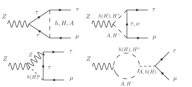
Figure 1: Representative Feynman diagrams for $Z\to\mu\tau$ decay.

Since many one-loop Feynman diagrams are involved in the process, we employ the FormCalc package Hahn:1998yk to deal with the loop calculations. The lengthy formulas are not shown here; instead, we directly show the numerical results.

Before presenting the numerical analysis, we discuss the theoretical and experimental constraints. The main theoretical constraints of THDM are the perturbative scalar potential, vacuum stability, and unitarity. Therefore, in order to satisfy the perturbative requirement, we set all quartic couplings of the scalar potential to obey $|\lambda_{i}|\leq 8\pi$ for all $i$. The conditions for vacuum stability are Sher:1988mj ; Ferreira:2004yd :

$$\lambda_{1}>0\;,\quad\quad\lambda_{2}>0\;,\lambda_{3}+\sqrt{\lambda_{1}\lambda_{2}}>0,\quad\sqrt{\lambda_{1}\lambda_{2}}+\lambda_{3}+\lambda_{4}-|\lambda_{5}|>0,$$

$${2|\lambda_{6}+\lambda_{7}|\leq\frac{1}{2}(\lambda_{1}+\lambda_{2})+\lambda_{3}+\lambda_{4}+\lambda_{5}}\,.$$ (27)

Without losing the general properties, we set $\lambda_{6,7}\ll 1$ in our numerical analysis. Effectively, the scalar potential is similar to that in the type II THDM. Since the unitarity constraint involves a variety of scattering processes, here we adopt the results of a previous study Akeroyd:2000wc .

Next, we briefly state the experimental bounds. It is known that $b\to s\gamma$ is sensitive to the mass of charged Higgs. According to a recent analysis Misiak:2015xwa , the lower bound in the type II model is given to be $m_{H^{\pm}}>480$ GeV at 95$\%$ CL. Due to the neutral and charged Higgses involved in the self-energy of W and Z bosons, the precision measurements of the $\rho$-parameter and the oblique parameters Peskin:1991sw can give constraints on the associated new parameters. From the global fit, we know that $\rho=1.00040\pm 0.00024$ PDG and the SM prediction is $\rho=1$. Taking $m_{h}=125$ GeV, $m_{t}=173.3$ GeV, and assuming $U=0$, the tolerated ranges for S and T are found to be Baak:2014ora :

$$\Delta S=0.06\pm 0.09\,,\ \ \Delta T=0.10\pm 0.07\,,$$ (28)

where the correlation factor is $\rho=+0.91$, $\Delta S=S^{\textrm{2HDM}}-S^{\textrm{SM}}$, $\Delta T=T^{\textrm{2HDM}}-T^{\textrm{SM}}$, and their explicit expressions can be found elsewhere Gunion:2002zf . We note that in the limit $m_{H^{\pm}}=m_{A}$ or $m_{H^{\pm}}=m_{H}$, $\Delta T$ vanishes Gerard:2007kn ; Cervero:2012cx .

Since the Higgs data approach the precision measurements, the relevant measurements can give strict limits on $c_{\beta\alpha}$ and $s_{\alpha}$. As usual, the Higgs measurement is expressed by the signal strength, which is defined by the ratio of the Higgs signal to the SM prediction, given by:

$$\mu^{f}_{i}=\frac{\sigma_{i}(h)\cdot BR(h\to f)}{\sigma^{SM}_{i}(h)\cdot BR^{SM}(h\to f)}\equiv\bar{\sigma}_{i}\cdot\mu_{f}\,.$$ (29)

$\sigma_{i}(h)$ denotes the Higgs production cross section by channel $i$ and $BR(h\to f)$ is the BR for the Higgs decay $h\to f$. Since several Higgs boson production channels are available at the LHC, we are interested in the gluon fusion production ($ggF$), $t\bar{t}h$, vector boson fusion (VBF) and Higgs-strahlung $Vh$ with $V=W/Z$; they are grouped to be $\mu^{f}_{ggF+t\bar{t}h}$ and $\mu^{f}_{VBF+Vh}$. The values of observed signal strengths are shown in Table. 1, where we used the notations $\widehat{\mu}^{f}_{ggF+t\bar{t}h}$ and $\widehat{\mu}^{f}_{VBF+Vh}$ to express the combined results of ATLAS atlas034 and CMS cms005 .

Table 1: Combined best-fit signal strengths $\widehat{\mu}_{\rm{ggF+tth}}$ and $\widehat{\mu}_{\rm{VBF+Vh}}$ and the associated correlation coefficient $\rho$ for corresponding Higgs decay mode atlas034 ; cms005 .

$f$	$\widehat{\mu}^{f}_{\rm{ggF+tth}}$	$\widehat{\mu}^{f}_{\rm{VBF+Vh}}$	$\pm\,\,1\widehat{\sigma}_{\rm{ggF+tth}}$	$\pm\,\,1\widehat{\sigma}_{\rm{VBF+Vh}}$	$\rho$
$\gamma\gamma$	$1.32$	0.8	0.38	0.7	-0.30
$ZZ^{*}$	$1.70$	0.3	0.4	1.20	-0.59
$WW^{*}$	$0.98$	1.28	0.28	0.55	-0.20
$\tau\tau$	$2$	1.24	1.50	0.59	-0.42
$b\bar{b}$	1.11	0.92	0.65	0.38	0

In order to study the influence of new free parameters and to understand their correlations, we employ the minimum $\chi$-square method with the experimental data considered. For a given Higgs decay channel $f=\gamma\gamma,WW^{*},ZZ^{*},\tau\tau$, we define the $\chi^{2}_{f}$ as:

$$\chi^{2}_{f}=\frac{1}{\hat{\sigma}^{2}_{1}(1-\rho^{2})}(\mu^{f}_{1}-\hat{\mu}^{f}_{1})^{2}+\frac{1}{\hat{\sigma}^{2}_{1}(1-\rho^{2})}(\mu^{f}_{2}-\hat{\mu}^{f}_{2})^{2}-\frac{2\rho}{\hat{\sigma}_{1}\hat{\sigma}_{2}(1-\rho^{2})}(\mu^{f}_{1}-\hat{\mu}^{f}_{1})(\mu^{f}_{2}-\hat{\mu}^{f}_{2})\,,$$ (30)

where $\hat{\mu}^{f}_{1(2)}$, $\hat{\sigma}_{1(2)}$, and $\rho$ are the measured Higgs signal strength, the one-sigma errors, and the correlation, respectively. The corresponding values are shown in Table 1. The indices $1$ and $2$ respectively stand for $\rm ggF+tth$ and $\rm VBF+Vh$, and $\mu^{f}_{1,2}$ are the results in the THDM. The global $\chi$-square is defined by

$$\chi^{2}=\sum_{f}\chi^{2}_{f}+\chi^{2}_{ST}\,,$$ (31)

where $\chi^{2}_{ST}$ is the $\chi^{2}$ for S and T parameters; its definition can be obtained from Eq.(30) by using the replacements $\mu^{f}_{1}\to S^{\rm THDM}$ and $\mu^{f}_{2}\to T^{\rm THDM}$, and the corresponding values can be determined from Eq. (28).

Besides the bounds from theoretical considerations, Higgs data, and upper limit $BR(\mu\to 3e)<1.0\times 10^{-12}$, the schemes for the setting of parameters in this study are as follows: the masses of SM Higgs and charged Higgs are fixed to be $m_{h}=125.5$ GeV and $m_{H^{\pm}}=500$ GeV, respectively, and the regions of other involved parameters are chosen as:

$$\quad m_{H,A}\supset[126,1000]\,{\rm GeV}\,,\quad m^{2}_{12}\supset[-1.0,1.5]\times 10^{5}\,{\rm GeV^{2}}\,,$$

$$\tan\beta\supset[0.5,50]\,,\quad\alpha=[-\pi/2,\pi/2]\,.$$ (32)

Since our purpose is to show the impacts of THDM on LFV, to lower the influence of the quark sector, we set ${\bf X}^{q}\sim 0$ in the current analysis; i.e., the Yukawa couplings of quarks behave like the type II THDM. The influence of $X^{q}\neq 0$ can be found elsewhere Arhrib:2015maa . To understand the small lepton FCNCs, we use the ansatz $X^{\ell}_{ij}=\sqrt{m_{i}m_{j}}/v\chi^{\ell}_{ij}$; thus, $\chi^{\ell}_{ij}$ can be on the order of one. Although $h$-$\ell^{+}$-$\ell^{-}$ couplings also contribute to the $h\to 2\gamma$ process, unless one makes an extreme tuning on $\chi^{\ell}_{ii}$, their contributions to $h\to 2\gamma$ are small in the THDM.

We now present the numerical analysis. Combining the theoretical requirements and $\delta\rho=(4.0\pm 2.4)\times 10^{-4}$, the allowed ranges of $\tan\beta$ and $c_{\beta\alpha}$ are shown by the yellow dots in Fig. 2 , where the scanned regions of Eq. (32) were used. When the measurements of oblique parameters are included, the allowed parameter space is changed slightly, as shown by blue dots in Fig. 2. In both cases, data with $2\sigma$ errors are adopted. From the results, we see that the constraint on $c_{\beta\alpha}$ is loose and the favorable range for $\tan\beta$ is $\tan\beta<20$.

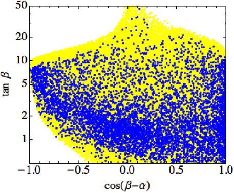
Figure 2: Constraints from theoretical requirements and precision measurement of $\rho$-parameter (yellow dots) and results (blue points) when measurements of oblique parameters are included.

To perform the constraints from Higgs data listed in Table 1, we use the minimum $\chi$-square approach. The best fit is taken at $68\%$, $95.5\%$, and $99.7\%$ CLs; that is, the corresponding errors of $\chi^{2}$ are $\Delta\chi^{2}\leq 2.3$, $5.99$, and $11.8$, respectively. With the definitions in Eqs. (30) and (31), we present the allowed values of parameters in Fig. 3(a), where the theoretical requirements, $\delta\rho$, oblique parameters, and Higgs data are all included. In the plots, blue, green, and red represent $68\%$, $95.5\%$, and $99.7\%$ CLs, respectively. It is clear that $c_{\beta\alpha}$ has been limited to a narrow range and that the favorable values of $\tan\beta$ are less than $10$. We can understand the correlation between angle $\beta$ and $\alpha$ from Fig. 3(b). We will use these results to study other rare decays.

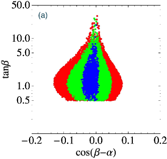
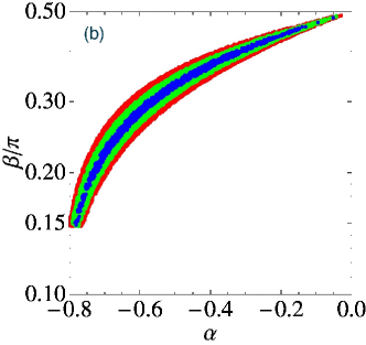
Figure 3: Bounds with $\chi$-square fit as a function of (a) $\tan\beta$ and $\cos(\beta-\alpha)$ and (b) $\beta/\pi$ and $\alpha$, where blue, green, and red denote $\Delta\chi^{2}\leq 2.3$, $5.99$ ,and $11.8$, respectively.

For calculating $\Delta a_{\mu}$ and rare tau, $\mu$, and $Z$ decays, we need information about the allowed masses of $H$ and $A$. Using the results of $\chi$-square fitting, we present the correlation between $m_{H}-m_{H^{\pm}}$ and $m_{A}-m_{H}$ in Fig. 4(a) and that between $m^{2}_{12}$ and $m_{A}-m_{H}$ in Fig. 4(b), where the ranges of parameters in Eq. (32) are satisfied.

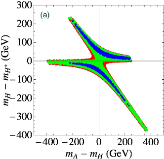
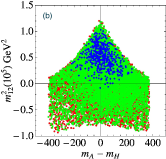
Figure 4: Correlations between (a) $m_{H}-m_{H^{\pm}}$ and $m_{A}-m_{H}$ and (b) $m^{2}_{12}$ and $m_{A}-m_{H}$, where blue, green, and red denote $\Delta\chi^{2}\leq 2.3$, $5.99$, and $11.8$, respectively.

After obtaining the allowed ranges of parameters, we analyze the implications of lepton-flavor-violating effects on $h\to\mu\tau$ and other rare decays. From Eq. (17), it can be seen that the $h\to\mu\tau$ decay is sensitive to $c_{\beta\alpha}$, $\tan\beta$, and $\chi^{\ell}_{23}$. In order to understand under what conditions the CMS results of $h\to\mu\tau$ can be reached in the type III THDM, we show the contour for $BR(h\to\mu\tau)=0.84\%$ as a function of $\tan\beta$ and $c_{\beta\alpha}$ in Fig. 5(a), where the solid and dashed lines stand for $\chi^{\ell}_{23}=4$ and $6$, respectively. We find that in order to fit the central value of the CMS results and satisfy the bounds from Higgs data simultaneously, one needs $\chi^{\ell}_{23}>5$. That is, with the severe limits of $\tan\beta$ and $c_{\beta\alpha}$, an accurate measurement of $h\to\mu\tau$ can directly bound the $\chi^{\ell}_{23}$. To clearly show the correlation between $BR(h\to\mu\tau)$ and the parameters constrained by Higgs data, we plot the $BR(h\to\mu\tau)$ in terms of the results of Fig. 3 in Fig. 5(b), where we fix $\chi^{\ell}_{23}=5$ and blue, green, and red stand for the best fits at 68%, 95%, and 99.7% CLs, respectively.

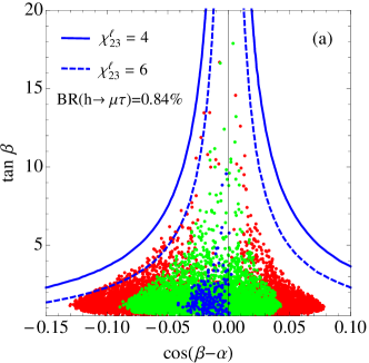
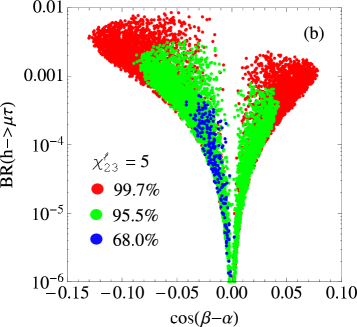
Figure 5: (a) Contour for $BR(h\to\mu\tau)=0.84\%$ as function of $\cos(\beta-\alpha)$ and $\tan\beta$ with $\chi^{\ell}_{23}=4$ (solid) and $6$ (dashed). (b) $BR(h\to\mu\tau)$ as function of $\cos(\beta-\alpha)$, where blue, green, and red stand for the best fits at $68\%$, $95\%$, and $99.7\%$ CLs, respectively.

From Eq. (19), we see that the tree-level $\tau\to 3\mu$ decay is sensitive to the masses of $m_{H,A}$, $\tan\beta$, and $\chi^{\ell}_{23,22}$, but insensitive to $c_{\beta\alpha}$. In Fig. 6(a), we show the contours for $BR(\tau\to 3\mu)\times 10^{8}$ as a function of $\tan\beta$ and $m_{H}$, where $m_{A}=300$ GeV, $\chi^{\ell}_{23}=5$, $\chi^{\ell}_{22}=-2$, and $c_{\beta\alpha}=-0.05$ are used. The values in the plot denote the BR for $\tau\to 3\mu$; the largest one is the current upper limit. Although a vanished $\chi^{\ell}_{22}$ still leads to a sizable $BR(\tau\to 3\mu)$, its value influences the BR for the $\tau\to 3\mu$ decay. To understand the effect of $\chi^{\ell}_{22}$, we plot $BR(\tau\to 3\mu)\times 10^{8}$ as a function of $\chi^{\ell}_{23}$ and $\chi^{\ell}_{22}$ in Fig. 6(b), where $\tan\beta=6$ and $m_{H(A)}=200(300)$ GeV. These parameter values are consistent with the constraints from Higgs data.

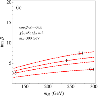
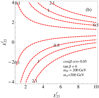
Figure 6: Contours for $BR(\tau\to 3\mu)\times 10^{8}$ as function of (a) $m_{H}$ and $\tan\beta$ with $\chi^{\ell}_{23(22)}=5(-2)$ and (b) $\chi^{\ell}_{23}$ and $\chi^{\ell}_{22}$ with $m_{H}=200$ GeV and $\tan\beta=6$. In both plots, $m_{A}=300$ GeV and $\cos(\beta-\alpha)=-0.05$.

From Eq. (38), it can be seen that besides the parameters $\tan\beta$, $m_{H,A}$ and $\chi^{\ell}_{23}$, $\tau\to\mu\gamma$ at the one-loop level is also dictated by $\chi^{\ell}_{33}$. Since $c_{\beta\alpha}$ has been limited to a narrow region, like the $\tau\to 3\mu$ decay, $\tau\to\mu\gamma$ is insensitive to $c_{\beta\alpha}$. We present the contours for $BR(\tau\to\mu\gamma)\times 10^{8}$ as a function of $\tan\beta$ and $m_{H}$ in Fig. 7(a), where we have included the one- and two-loop contributions and $c_{\beta\alpha}=-0.05$, $\chi^{\ell}_{23(33)}=5(0)$, and $m_{A}=300$ GeV. The largest value on the curves is the current experimental upper limit. We see that with strict constraints of Higgs data, $BR(\tau\to\mu\gamma)$ in the typeIII THDM can still be compatible with the current upper limit when the decay $h\to\mu\tau$ matches CMS observation.

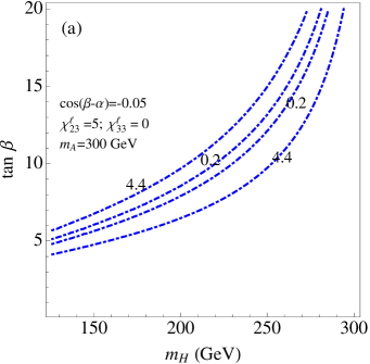
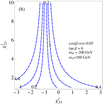
Figure 7: Contours for $BR(\tau\to\mu\gamma)\times 10^{8}$ as function of (a) $\tan\beta$ and $m_{H}$ with $\chi^{\ell}_{23}(\chi^{\ell}_{33})=5(0)$ and (b) $\chi^{\ell}_{23}$ and $\chi^{\ell}_{33}$ with $\tan\beta=6$ and $m_{H(A)}=200(300)$ GeV. One- and two-loop effects are included.

According to Eq. (21), we know that muon $g-2$ strongly depends on $\chi^{\ell}_{23}$, $\tan\beta$, and $m_{H,A}$. It is of interest to determine whether $\Delta a_{\mu}$ could be explained by the type III model when the severe limits of involved parameters are imposed. With $m_{A}=300$ GeV, $\chi^{\ell}_{23}=5$, we plot the contours for $\Delta a_{\mu}\times 10^{9}$ as a function of $\tan\beta$ and $m_{H}$ in Fig. 8(a), where the shaded region (yellow) stands for the central value with $2\sigma$ errors. From the plot, it is clear that these parameter values, which satisfy the Higgs data and $BR(h\to\mu\tau)=0.84\%$ can also make $(g-2)_{\mu}$ consistent with the discrepancy between the experimental data and SM prediction. Based on Eq. (25), it is found that $\mu\to e\gamma$ can be expressed by $\Delta a_{\mu}$. With the ansatz $X^{\ell}_{ij}=\sqrt{m_{i}m_{j}}/v\chi^{\ell}_{ij}$, we show the contours for $BR(\mu\to e\gamma)$ as a function of $\Delta a_{\mu}$ and $\chi^{\ell}_{13}/\chi^{\ell}_{23}$ in Fig. 8(b), where the numbers on the curves are the BR for $\mu\to e\gamma$ decay obtained by multiplying $10^{13}$. Clearly, in order to satisfy the bound from the rare $\mu\to e\gamma$ decay, $\chi^{\ell}_{13}$ has to be less than ${\cal O}(10^{-3})$. As a result, we get:

$$BR(h\to e\tau)<2\times 10^{-4}\left(\frac{\chi^{\ell}_{13}/\chi^{\ell}_{23}}{10^{-3}}\right)^{2}BR(h\to\mu\tau).$$ (33)

Hence, in the type III THDM, $h\to e\tau$ at least is an order of $10^{4}$ smaller than $h\to\mu\tau$.

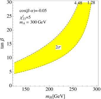
Figure 8: (a) Contours for $\Delta a_{\mu}\times 10^{9}$ as function of $\tan\beta$ and $m_{H}$ with $m_{A}=300$ GeV, $\chi^{\ell}_{23}=5$, and $\cos(\beta-\alpha)=-0.05$ and (b) contours for $BR(\mu\to e\gamma)\times 10^{13}$ as a function of $\Delta a_{\mu}$ and $\chi^{\ell}_{13}/\chi^{\ell}_{23}$, where relation in Eq. (25) is adopted.

Finally, we discuss the decay $Z\to\mu\tau$. Similar to rare $\tau$ decays, $BR(Z\to\mu\tau)$ is sensitive to $\tan\beta$, $m_{H,A}$, and $\chi^{\ell}_{23(33)}$ in the type III model. Although we do not explicitly show the formulas in this paper, we present the contours for $BR(Z\to\mu\tau)\times 10^{7}$ as a function of $\tan\beta$ and $m_{H}$ in Fig. 9(a), where $m_{A}=300$ GeV, $\chi^{\ell}_{23(33)}=5(0)$, and $c_{\beta\alpha}=-0.05$ are used. With the constrained parameters that fit the CMS results of $h\to\mu\tau$, we find that BR for $Z\to\mu\tau$ decay is $BR(Z\to\mu\tau)<10^{-6}$. The current experimental upper limit is $BR(Z\to\mu\tau)^{\rm exp}<2.1\times 10^{-5}$. To understand the dependence of $\chi^{\ell}_{23}$, we also show the contours as a function of $\tan\beta$ and $\chi^{\ell}_{23}$ with $m_{H}=200$ GeV in Fig. 9(b).

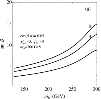
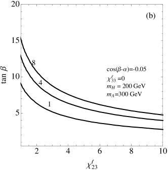
Figure 9: Contours for $BR(Z\to\mu\tau)\times 10^{7}$ as function of (a) $\tan\beta$ and $m_{H}$ with $\chi^{\ell}_{23}=5$ and (b) $\tan\beta$ and $\chi^{\ell}_{23}$ with $m_{H}=200$ GeV. In both plots, we adopt $m_{A}=300$ GeV, $\chi^{\ell}_{33}=0$, and $\cos(\beta-\alpha)=-0.05$.

In summary, we revisited the constraints for THDM. The bounds from theoretical requirements, precision $\delta\rho$, and oblique parameter measurements are shown in Fig. 2 and the bounds from Higgs data with $\chi$-square fit at $68\%$, $95.5\%$, and $99.7\%$ CLs are given in Fig. 3. We clearly show the tension of Higgs data on the parameters of new physics. With the parameter values constrained by Higgs data, we find that the type III THDM can fit the CMS result $BR(h\to\mu\tau)=(0.84^{+0.39}_{-0.37})\%$. With the same set of parameters, the resultant branching ratios of tree-level $\tau\to 3\mu$ and loop-induced $\tau\to\mu\gamma$ decays are consistent with the current experimental upper limits. Under the strict limits of Higgs data, we clearly show that the anomaly of the muon anomalous magnetic moment can be explained by the type III model. The rare decay $\mu\to e\gamma$ can be satisfied by small parameter $\chi^{\ell}_{13}$. As a result, we expect that the branching ratio for $h\to e\tau$ is smaller than that for the decay $h\to\mu\tau$ by an order of magnitude of $10^{4}$. Additionally, we also calculated the branching ratio for rare decay $Z\to\mu\tau$ and the result is one order of magnitude smaller than the current experimental upper limit.

Acknowledgments

The work of CHC was supported by the Ministry of Science and Technology of Taiwan, R.O.C., under grant MOST-103-2112-M-006-004-MY3. The work of RB was supported by the Moroccan Ministry of Higher Education and Scientific Research MESRSFC and CNRST: ”Projet dans les domaines prioritaires de la recherche scientifique et du développement technologique”: PPR/2015/6.

Appendix A

A.1 Yukawa couplings

The Higgs Yukawa couplings to fermions are expressed as:

$$-{\cal L}^{h}_{Y} = \bar{u}_{L}\left[\frac{c_{\alpha}}{vs_{\beta}}{\bf m_{u}}-\frac{c_{\beta\alpha}}{s_{\beta}}{\bf X}^{u}\right]u_{R}h+\bar{d}_{L}\left[-\frac{s_{\alpha}}{vc_{\beta}}{\bf m_{d}}+\frac{c_{\beta\alpha}}{c_{\beta}}{\bf X}^{d}\right]d_{R}h$$ (34)

$$+ \bar{\ell}_{L}\left[-\frac{s_{\alpha}}{vc_{\beta}}{\bf m_{\ell}}+\frac{c_{\beta\alpha}}{c_{\beta}}{\bf X}^{\ell}\right]\ell_{R}h+h.c.\,,$$

where $c_{\beta\alpha}=\cos(\beta-\alpha)$, $s_{\beta\alpha}=\sin(\beta-\alpha)$ and ${\bf X}^{f}s$ are defined in Eq. (15). Similarly, the Yukawa couplings of scalars $H$ and $A$ are expressed as:

$$-{\cal L}^{H,A}_{Y} = \bar{u}_{L}\left[\frac{s_{\alpha}}{vs_{\beta}}{\bf m_{u}}+\frac{s_{\beta\alpha}}{s_{\beta}}{\bf X}^{u}\right]u_{R}H+\bar{d}_{L}\left[\frac{c_{\alpha}}{vc_{\beta}}{\bf m_{d}}-\frac{s_{\beta\alpha}}{c_{\beta}}{\bf X}^{d}\right]d_{R}H$$ (35)

$$+ \bar{\ell}_{L}\left[\frac{c_{\alpha}}{vc_{\beta}}{\bf m_{\ell}}-\frac{s_{\beta\alpha}}{c_{\beta}}{\bf X}^{\ell}\right]\ell_{R}H+i\bar{u}_{L}\left[-\frac{\cot\beta}{v}{\bf m_{u}}+\frac{{\bf X}^{u}}{s_{\beta}}\right]u_{R}A$$

$$+ i\bar{d}_{L}\left[-\frac{\tan\beta}{v}{\bf m_{d}}+\frac{{\bf X}^{d}}{c_{\beta}}\right]d_{R}A+i\bar{\ell}_{L}\left[-\frac{\tan\beta}{v}{\bf m_{\ell}}+\frac{{\bf X}^{\ell}}{c_{\beta}}\right]\ell_{R}A+h.c.$$

The Yukawa couplings of charged Higgs to fermions are:

$$-{\cal L}^{H^{\pm}}_{Y} = \sqrt{2}\bar{d}_{L}V^{\dagger}_{CKM}\left[-\frac{\cot\beta}{v}{\bf m_{u}}+\frac{{\bf X}^{u}}{s_{\beta}}\right]u_{R}H^{-}$$ (36)

$$+ \sqrt{2}\bar{u}_{L}V_{\rm CKM}\left[-\frac{\tan\beta}{v}{\bf m_{d}}+\frac{{\bf X}^{d}}{c_{\beta}}\right]d_{R}H^{+}$$

$$+ \sqrt{2}\bar{\nu}_{L}V_{\rm PMNS}\left[-\frac{\tan\beta}{v}{\bf m_{\ell}}+\frac{{\bf X}^{\ell}}{c_{\beta}}\right]\ell_{R}H^{+}+h.c.\,,$$

where CKM and PMNS stand for Cabibbo-Kobayashi-Maskawa and Pontecorvo-Maki-Nakagawa-Sakata matrices, respectively. Except the factor $\sqrt{2}$ and CKM matrix, the Yukawa couplings of charged Higgs are the same as those of pseudoscalar $A$.

A.2 $\tau\to\mu\gamma$ decay

The effective interaction for $\tau\to\mu\gamma$ is expressed by

$${\cal L}_{\tau\to\mu\gamma}=\frac{e}{16\pi^{2}}m_{\tau}\bar{\mu}\sigma_{\mu\nu}\left(C^{\prime}_{L}P_{L}+C^{\prime}_{R}P_{R}\right)\tau F^{\mu\nu}\,,$$ (37)

where the Wilson coefficients $C^{\prime}_{L}$ and $C^{\prime}_{R}$ from the one-loop neutral and charged scalars are formulated as:

$$C^{\prime}_{L(R)} =\sum_{\phi=h,H,A,H^{\pm}}C^{\prime\phi}_{L(R)}\,,$$

$$C^{\prime h}_{L} =\frac{c_{\beta\alpha}X^{\ell}_{32}}{2m^{2}_{h}c_{\beta}}y^{\ell}_{h33}\left(\ln\frac{m^{2}_{h}}{m^{2}_{\tau}}-\frac{4}{3}\right)\,,\ C^{\prime H}_{L}=\frac{-s_{\beta\alpha}X^{\ell}_{32}}{2m^{2}_{H}c_{\beta}}y^{\ell}_{H33}\left(\ln\frac{m^{2}_{H}}{m^{2}_{\tau}}-\frac{4}{3}\right)\,,$$

$$C^{\prime A}_{L} =-\frac{X^{\ell}_{32}}{2m^{2}_{A}c_{\beta}}y^{\ell}_{A33}\left(\ln\frac{m^{2}_{A}}{m^{2}_{\tau}}-\frac{5}{3}\right)\,,\ C^{\prime H^{\pm}}_{L}=-\frac{1}{12m^{2}_{H^{\pm}}}\left(\frac{\sqrt{2}X^{\ell}_{32}}{c_{\beta}}\right)y^{\ell}_{H^{\pm}33}\,,$$ (38)

$C^{\prime h,H,A}_{R}=C^{\prime h,H,A}_{L}$ and $C^{\prime H^{\pm}}_{R}=0$. In addition, the contributions from two loops are given by Sierra:2014nqa ; Chang:1993kw ; Davidson:2010xv

$$C^{ht(b)}_{2L} =C^{ht(b)}_{2R}=2\frac{c_{\beta\alpha}X_{32}y^{u(d)}_{h33}}{c_{\beta}}\frac{N_{c}Q_{f}^{2}\alpha}{\pi}\frac{1}{m_{\tau}m_{t(b)}}f\left(\frac{m_{t(b)}^{2}}{m_{h}^{2}}\right)\,,$$

$$C^{Ht(b)}_{2L} =C^{Ht(b)}_{2R}=-2\frac{s_{\beta\alpha}X_{32}y^{u(d)}_{H33}}{c_{\beta}}\frac{N_{c}Q_{f}^{2}\alpha}{\pi}\frac{1}{m_{\tau}m_{t(b)}}f\left(\frac{m_{t(b)}^{2}}{m_{H}^{2}}\right)\,,$$

$$C^{At(b)}_{2L} =C^{At(b)}_{2R}=-2\frac{X_{32}y^{u(d)}_{A33}}{c_{\beta}}\frac{N_{c}Q_{f}^{2}\alpha}{\pi}\frac{1}{m_{\tau}m_{t(b)}}f\left(\frac{m_{t(b)}^{2}}{m_{A}^{2}}\right)\,,$$

$$C^{W}_{2L} =C^{W}_{2R}=\frac{s_{\beta\alpha}c_{\beta\alpha}X_{32}}{c_{\beta}}\frac{g\alpha}{2\pi m_{\tau}m_{W}}\Bigl{[}3f\left(\frac{m_{W}^{2}}{m_{H}^{2}}\right)+\frac{23}{4}g\left(\frac{m_{W}^{2}}{m_{H}^{2}}\right)+\frac{3}{4}h\left(\frac{m_{W}^{2}}{m_{H}^{2}}\right)$$

$$\hskip 142.26378pt+\frac{m_{H}^{2}}{2m_{W}^{2}}\left(f\left(\frac{m_{W}^{2}}{m_{H}^{2}}\right)-g\left(\frac{m_{W}^{2}}{m_{H}^{2}}\right)\right)\Bigr{]}-(m_{H}\rightarrow m_{h})\,,$$ (39)

where the loop functions are

$$f(z) =\frac{z}{2}\int^{1}_{0}dx\frac{(1-2x(1-x))}{x(1-x)-z}\ln\frac{x(1-x)}{z}\,,$$

$$g(z) =\frac{z}{2}\int^{1}_{0}dx\frac{1}{x(1-x)-z}\ln\frac{x(1-x)}{z}\,,$$

$$h(z) =-\frac{z}{2}\int^{1}_{0}dx\frac{1}{x(1-x)-z}\left[1-\frac{z}{x(1-x)-z}\ln\frac{x(1-x)}{z}\right]\,.$$ (40)

The BR for $\tau\to\mu\gamma$ is expressed by

$$\frac{BR(\tau\to\mu\gamma)}{BR(\tau\to\mu\bar{\nu}_{\mu}\nu_{\tau})}=\frac{3\alpha_{e}}{4\pi G^{2}_{F}}\left(|C^{\prime}_{L}|^{2}+|C^{\prime}_{R}|^{2}\right)\,.$$ (41)